Stabilizing radion and dilaton with brane gas and flux

Abstract

We consider the dynamics of moduli fields in brane gas cosmology. By calculating the effective potentials from brane gas and bulk RR field, we found an attractor behavior that can fix both the radion and the dilaton. The potentials for radion and dilaton show global minima that can provide the stabilizing forces so that they can be stabilized dynamically. The effective potential for the three-dimensional volume is runaway-type so that it can inflate.

I Introduction

The primary goal of string cosmology is to find a successful compactification that can produce inflation consistent with current observations. The physical quantities characterizing the shape or the size of extra dimensions are called moduli. In the point of four dimensional theory, the existence of moduli appears as scalar fields. They play important roles in supergravity models obtained as low energy limit of superstring theory. For example, since the vacuum expectation value of the dilaton determines the strength of the gravitational coupling, a rolling dilaton implies a changing gravitational constant. Also the extra dimensions should be compact and small through the cosmological evolution of the early universe. Thus the volume modulus of the extra dimensions (radion) should be stabilized in any cosmological models in order not to conflict with current observations. To stabilize the moduli fields in string theory, various models and mechanisms were introduced (see silverstein and references therein).

One way to achieve the moduli stabilization is adopting the framework of string/brane gas cosmology based on the mechanism of Brandenberger and Vafa bv ; abe . In the study of string cosmology it is found that a gas of extended objects (strings and branes) could affect the evolution of the universe in the presence of nontrivial topology. A gas of strings or branes can be coupled to a cosmological background in the same way as a gas of point particles is coupled to a background of standard Einstein gravity. Many of the works on string/brane gas cosmology were concentrated on the stabilization of the radion assuming that the dilaton can be stabilized by some other mechanism wb0307044 ; pb ; bw0403075 ; watson ; cwb ; campos ; rador0504047 ; patil ; kaya ; eastro ; chatrabhuti ; kim0608131 ; akk ; kim08040073 .

Some of the key factors that can specify the cosmological evolution in string cosmology are the spacetime dimensionality, the geometry and topology, the location of sources, orientifold planes, and fluxes. In the previous work kim08040073 , we evaluated the effective potentials, induced by brane gas, bulk flux, and supergravity particles, that govern the sizes of the observed three and extra six dimensions. We found that the internal volume can oscillate between two turning points or sit at the minimum of the potential while the three-dimensional volume expands indefinitely. However, in string or brane cosmology, one has to study the dynamics involving both the radion and the dilaton bc ; bbc ; bbem ; ks ; cw ; rador0701029 ; sano since branes in general couple to both the dilaton and the radion. Recently it has been studied that a nonperturbatively generated potential by gaugino condensation and a gas of strings can stabilize both the dilaton and the radial modulus in heterotic string theory dfb .

The motivation of this paper is to study how the running of the dilaton affects the behavior of the three-dimensional volume factor and the radion. It is already known that the bulk fluxes can generate potentials to stabilize the moduli in string theory drs ; gkp and in Randall-Sundrum scenario gw . We will make use of a bulk Ramond-Ramond (RR) flux to stabilize simultaneously both the dilaton and the radion in brane gas formalism of type II string theory. We will show that it is possible to stabilize both moduli dynamically by an attractor mechanism, while the three-dimensional volume can expand monotonically. The crucial point is that the coupling of dilaton to brane and RR gauge field induces confining potentials for stabilization.

The paper is organized as follows. In Sec. II, we consider a cosmological formalism based on the dilaton gravity with a four-form bulk RR flux and a six-dimensional brane gas. In Sec. III, we set up the equations of motion for the dilaton, the six-dimensional internal subspace, and the three-dimensional subspace. Then we reduce them to motions of a particle under an effective potential. We will show that the radion and the dilaton can be stabilized separately if one of the two is fixed. In Sec. IV, we consider the dynamical stabilization of the two fields. In Sec. V, we conclude and discuss.

II Equations of motion

In the point of string theory, the gravitational interaction is described by the coupled system of metric and dilaton. We consider the dilaton cosmology with a bulk RR flux and a brane gas. To be specific, let us start from the following bulk effective action of type II string theory kim0608131

$$S_{\rm b}=\frac{1}{2\kappa^{2}}\int d^{D+1}x\sqrt{-g}\Bigl{[}e^{-2\phi}\{R+4(\nabla\phi)^{2}\}-\frac{1}{2\cdot 4!}F_{4}^{2}-V(\phi)\Bigr{]},$$ (1)

where $\kappa^{2}=1/M^{D-1}_{*}$, with $M_{*}$ being the $(D+1)$-dimensional unification scale, $\phi$ is the dilaton field, $F_{4}$ is the four-form RR field strength, and $V(\phi)$ is the dilaton potential. Although we will consider the $D=9$ case, we will keep $D$ to see the dimensional dependence of our analysis.

We suppose that the matter contribution of a single brane to the action is represented by the Dirac-Born-Infeld (DBI) action of a $p$-brane

$$S_{\rm p-brane}=-T_{p}\int d^{p+1}\xi e^{-\phi}\sqrt{-{\rm det}({\hat{g}}_{\mu\nu}+{\hat{B}}_{\mu\nu}+2\pi\alpha^{\prime}{F}_{\mu\nu})},$$ (2)

where $T_{p}$ is the tension of the $p$-brane and ${\hat{g}}_{\mu\nu}$ is the induced metric to the brane

$${\hat{g}}_{\mu\nu}=g_{MN}\frac{\partial x^{M}}{\partial\xi^{\mu}}\frac{\partial x^{N}}{\partial\xi^{\nu}}.$$ (3)

Here $M$ and $N$ are the indices of bulk spacetime and $\mu$ and $\nu$ are those of brane. ${\hat{B}}_{\mu\nu}$ is the induced antisymmetric tensor field and ${F}_{\mu\nu}$ is the field strength tensor of gauge field $A_{\mu}$ living on the brane. The fluctuations of the fields within the brane are negligible when the temperature is low enough. Thus we neglect ${\hat{B}}_{\mu\nu}$ and ${F}_{\mu\nu}$ terms. Since the DBI action couples to both the dilaton and the radion, the brane action not only acts as a source term for gravity but also provides potentials for dilaton and radion.

We consider the case that the RR flux is laid on the three dimensions where windings of brane are removed completely, while the remaining six dimensions are wrapped with gases of branes whose dimensions are less than or equal to $(D-3)$. In general, the action of these gases can be written as a sum over the contributions of the gas from each string or brane state. The individual contribution is obtained by its number density and energy in a hydrodynamical approximation. However, assuming that each type of brane gas makes a comparable contribution, we consider a gas of effective $(D-3)$-branes whose tension we denote by $T_{D-3}$. In other words, we consider the effect of all lower-dimensional ($\leq D-3$) brane gas as a $(D-3)$-brane gas. The total action can be written as

$$S_{\rm tot}=S_{\rm b}+S_{\rm(D-3)-brane}.$$ (4)

Since the presence of moduli dependence in the Einstein term can cause an extra tadpole for moduli from the curvature, it is convenient to rescale the metric so that the Einstein term $\int\sqrt{g}{\cal R}$ is completely decoupled from other moduli. To solve the field equations we work in the ten-dimensional Einstein frame, defined by

$$g_{MN}^{\rm S}=e^{\frac{1}{2}\phi}g_{MN}^{\rm E}.$$ (5)

In terms of the Einstein metric, the action can be written as

$$S_{\rm b}^{E}=\frac{1}{2\kappa^{2}}\int d^{D+1}x\sqrt{-g^{E}}\Bigl{[}\{R-\frac{1}{2}(\nabla\phi)^{2}\}-\frac{e^{\frac{1}{2}\phi}}{2\cdot 4!}F_{4}^{2}-V_{E}(\phi)\Bigr{]},$$ (6)

$$S_{\rm(D-3)-brane}^{E}=-T_{D-3}\int d^{D-2}\xi e^{\frac{3}{4}\phi}\sqrt{-{\rm det}{\hat{g}}_{\mu\nu}^{E}},$$ (7)

where $V_{E}=e^{\frac{5}{2}\phi}V(\phi)$. We drop the superscript $E$ from now on. If one solves the field equation for $F_{4}$ in the Einstein frame, the $F_{4}^{2}$ term in Eq. (6) can give potential terms for dilaton and radion.

In the point of bulk theory, the energy momentum tensor of a single $(D-3)$-brane has a delta function singularity at the position of the brane along the transverse directions

$$\sqrt{-g}T_{\rm(D-3)-brane}^{MN}=-T_{D-3}\int d^{D-2}\xi e^{\frac{3}{4}\phi}\sqrt{-{\hat{g}}}{\hat{g}}^{\mu\nu}\partial_{\mu}x^{M}\partial_{\nu}x^{N}\delta(x-x(\xi)).$$ (8)

For cosmological setting, it seems natural to take a gas of such branes in a continuum approximation and this smooths the singularity by integrating over the transverse dimensions.

Since the dilaton potential is not known in string theory, we consider the simple case where the dilaton potential in the Einstein frame is a constant $V_{E}(\phi)=\Lambda$ to incorporate the cosmological constant. We will not consider its origin in detail here. With the metric ansatz

$$ds^{2}=-n^{2}dt^{2}+\sum_{k=1}^{D}a^{2}_{k}(t)(dx^{k})^{2},$$

the induced metric on the brane is

$${\hat{g}}_{\mu\nu}={\rm diag}\{-(1-v^{2}),a_{1}^{2},a_{2}^{2},a_{3}^{2}\},$$ (9)

where $v^{2}=\sum_{i=4}^{D}{\dot{x}}^{i}{\dot{x}}_{i}\geq 0$. If we consider the static brane ($v=0$), i.e., consider the brane does not move in the transverse directions, the brane time is the same as the bulk time.

Taking the following form of RR field

$$F_{N_{1},\cdots,N_{4}}=n\sqrt{4}\epsilon_{N_{1},\cdots,N_{3}}\nabla_{0}A(t),$$ (10)

where $N_{1},\cdots,N_{3}\neq 0$, the Bianchi identity,

$$\nabla_{[N}F_{N_{1},\cdots,N_{4}]}=0,$$ (11)

is automatically satisfied since $A(t)$ is a function of $t$ only. Then the one-dimensional effective action for the scale factors and the dilaton can be written as

$$S_{\rm eff}= - {\cal V}_{D}\int dt~{}nV_{D}\Bigl{[}\frac{1}{2\kappa^{2}}\Bigl{\{}\Bigl{(}\sum_{j=1}^{D}\frac{\dot{a}_{j}}{na_{j}}\Bigr{)}^{2}-\sum^{D}_{j=1}\Bigl{(}\frac{\dot{a}_{j}}{na_{j}}\Bigr{)}^{2}-\frac{1}{2}\frac{{\dot{\phi}}^{2}}{n^{2}}\Bigr{\}}$$ (12)

$$+ \Lambda+\frac{T_{D-3}}{V_{3}}e^{\frac{3}{4}\phi}-\frac{1}{2}\frac{e^{\frac{1}{2}\phi}}{V_{3}^{2}}{\dot{A}}^{2}\Bigr{]},$$

where ${\cal V}_{D}$ is the coordinate spatial volume, $V_{D}=\prod_{k=1}^{D}a_{k}$, and $V_{3}=\prod_{k=1}^{3}a_{k}$

To get the equations of motion, vary this action with respect to $n$, $a_{k}$, $\phi$, and ${\dot{A}}$, then set $n=1$ at the end. After some straightforward algebra, we obtain the following set of equations of motion:

$$\frac{1}{2\kappa^{2}}\Bigl{\{}\Bigl{(}\sum_{j=1}^{D}\frac{\dot{a}_{j}}{a_{j}}\Bigr{)}^{2}-\sum_{j=1}^{D}\Bigl{(}\frac{\dot{a}_{j}}{a_{j}}\Bigr{)}^{2}-\frac{1}{2}{\dot{\phi}}^{2}\Bigr{\}}=\Lambda+T_{D-3}\frac{e^{\frac{3}{4}\phi}}{V_{3}}+\frac{1}{2}\frac{e^{\frac{1}{2}\phi}}{V_{3}^{2}}{\dot{A}}^{2},$$ (13)

$$\frac{\ddot{a}_{n}}{a_{n}}+\sum_{l\neq n}\frac{\dot{a}_{n}\dot{a}_{l}}{a_{n}a_{l}}=\frac{\kappa^{2}}{D-1}\Bigl{\{}2\Lambda+(D-2)T_{D-3}\frac{e^{\frac{3}{4}\phi}}{V_{3}}+3\frac{e^{\frac{1}{2}\phi}}{V_{3}^{2}}{\dot{A}}^{2}\Bigr{\}}$$

$$-\kappa^{2}\Bigl{\{}T_{D-3}\frac{e^{\frac{3}{4}\phi}}{V_{D}}a_{n}\frac{\partial V_{D-3}}{\partial a_{n}}-\frac{1}{2}e^{\frac{1}{2}\phi}{\dot{A}}^{2}a_{n}\frac{\partial}{\partial a_{n}}\Bigl{(}\frac{1}{V_{3}^{2}}\Bigr{)}\Bigr{\}},$$ (14)

$${\ddot{\phi}}+\Bigl{(}\sum_{j=1}^{D}\frac{\dot{a}_{j}}{a_{j}}\Bigr{)}\dot{\phi}+2\kappa^{2}\Bigl{(}\frac{3}{4}T_{D-3}\frac{e^{\frac{3}{4}\phi}}{V_{3}}-\frac{1}{4}\frac{e^{\frac{1}{2}\phi}}{V_{3}^{2}}{\dot{A}}^{2}\Bigr{)}=0,$$ (15)

$$\frac{d}{dt}\Bigl{(}V_{D}\frac{e^{\frac{1}{2}\phi}}{V_{3}^{2}}{\dot{A}}\Bigr{)}=0.$$ (16)

Note that the derivative operator $a_{n}\frac{\partial}{\partial a_{n}}$ behaves like a counting operator. When it acts on $V_{3}$, it gives 1 for $n=1,2,3$ and 0 for $n=4,\cdots,D$.

The solution of (16) is given by

$${\dot{A}}=Q\frac{V_{3}^{2}}{V_{D}}e^{-\frac{1}{2}\phi},$$ (17)

with an integration constant $Q$. Substituting (17), the equations of motion (13)-(15) can be written as

$$\frac{1}{2\kappa^{2}}\Bigl{\{}\Bigl{(}\sum_{j=1}^{D}\frac{\dot{a}_{j}}{a_{j}}\Bigr{)}^{2}-\sum_{j=1}^{D}\Bigl{(}\frac{\dot{a}_{j}}{a_{j}}\Bigr{)}^{2}-\frac{1}{2}{\dot{\phi}}^{2}\Bigr{\}}=\Lambda+T_{D-3}\frac{e^{\frac{3}{4}\phi}}{V_{3}}+\frac{1}{2}Q^{2}\frac{e^{-\frac{1}{2}\phi}}{V_{D-3}^{2}},$$ (18)

$$\frac{\ddot{a}_{n}}{a_{n}}+\sum_{l\neq n}\frac{\dot{a}_{n}\dot{a}_{l}}{a_{n}a_{l}}=\frac{\kappa^{2}}{D-1}\Bigl{\{}2\Lambda+(D-2)T_{D-3}\frac{e^{\frac{3}{4}\phi}}{V_{3}}+3Q^{2}\frac{e^{-\frac{1}{2}\phi}}{V_{D-3}^{2}}\Bigr{\}}$$

$$-\kappa^{2}\Bigl{\{}T_{D-3}\frac{e^{\frac{3}{4}\phi}}{V_{D}}a_{n}\frac{\partial V_{D-3}}{\partial a_{n}}-\frac{1}{2}Q^{2}e^{-\frac{1}{2}\phi}\frac{V_{3}^{2}}{V_{D-3}^{2}}a_{n}\frac{\partial}{\partial a_{n}}\Bigl{(}\frac{1}{V_{3}^{2}}\Bigr{)}\Bigr{\}},$$ (19)

$${\ddot{\phi}}+\Bigl{(}\sum_{j=1}^{D}\frac{\dot{a}_{j}}{a_{j}}\Bigr{)}\dot{\phi}+2\kappa^{2}\Bigl{(}\frac{3}{4}T_{D-3}\frac{e^{\frac{3}{4}\phi}}{V_{3}}-\frac{1}{4}Q^{2}\frac{e^{-\frac{1}{2}\phi}}{V_{D-3}^{2}}\Bigr{)}=0.$$ (20)

To simplify the analysis we assume that the three-dimensional space and the internal $(D-3)$-dimensional space are isotropic so that $a_{1}=\cdots=a_{3}=a$ and $a_{4}=\cdots=a_{D}=b$. With this assumption, we have

$$6\Bigl{(}\frac{\dot{a}}{a}\Bigr{)}^{2}+(D-3)(D-4)\Bigl{(}\frac{\dot{b}}{b}\Bigr{)}^{2}+6(D-3)\frac{\dot{a}\dot{b}}{ab}-\frac{1}{2}{\dot{\phi}}^{2}$$

$$=2\kappa^{2}\Bigl{\{}\Lambda+T_{D-3}\frac{e^{\frac{3}{4}\phi}}{a^{3}}+\frac{1}{2}Q^{2}\frac{e^{-\frac{1}{2}\phi}}{b^{2(D-3)}}\Bigr{\}},$$ (21)

$$\frac{\ddot{a}}{a}+2\Bigl{(}\frac{\dot{a}}{a}\Bigr{)}^{2}+(D-3)\frac{\dot{a}\dot{b}}{ab}$$

$$=\frac{2\kappa^{2}}{D-1}\Lambda+\frac{D-2}{D-1}\kappa^{2}T_{D-3}\frac{e^{\frac{3}{4}\phi}}{a^{3}}-\frac{D-4}{D-1}\kappa^{2}Q^{2}\frac{e^{-\frac{1}{2}\phi}}{b^{2(D-3)}},$$ (22)

$$\frac{\ddot{b}}{b}+(D-4)(\frac{\dot{b}}{b})^{2}+3\frac{\dot{a}\dot{b}}{ab}$$

$$=\frac{2\kappa^{2}}{D-1}\Lambda-\frac{\kappa^{2}}{D-1}T_{D-3}\frac{e^{\frac{3}{4}\phi}}{a^{3}}+\frac{3}{D-1}\kappa^{2}Q^{2}\frac{e^{-\frac{1}{2}\phi}}{b^{2(D-3)}},$$ (23)

$${\ddot{\phi}}+\Big{\{}3\frac{\dot{a}}{a}+(D-3)\frac{\dot{b}}{b}\Big{\}}\dot{\phi}=-2\kappa^{2}\Bigl{\{}\frac{3}{4}T_{D-3}\frac{e^{\frac{3}{4}\phi}}{a^{3}}-\frac{1}{4}Q^{2}\frac{e^{-\frac{1}{2}\phi}}{b^{2(D-3)}}\Bigr{\}}.$$ (24)

Sources of positive energy in string cosmology tend to yield a runaway behavior, driving the volume to expand. A stable or metastable point is possible only in the presence of counterbalancing forces. We will search the possible solutions where $a$ becomes large indefinitely while both $b$ and $\phi$ remain finite.

III Effective potentials

For simplicity, we set $2\kappa^{2}=1$ because this factor can be absorbed into the redefinitions of $\Lambda$, $T_{D-3}$, and $Q^{2}$. Defining the two volumes of $SO(3)$ and $SO(D-3)$ subspaces as

$$\zeta\equiv a^{3},~{}~{}~{}~{}\xi\equiv b^{D-3},$$ (25)

the equations of motion can be written as

$$\frac{2}{3}\Bigl{(}\frac{\dot{\zeta}}{\zeta}\Bigr{)}^{2}+\frac{D-4}{D-3}\Bigl{(}\frac{\dot{\xi}}{\xi}\Bigr{)}^{2}+2\frac{\dot{\zeta}\dot{\xi}}{\zeta\xi}-\frac{1}{2}{\dot{\phi}}^{2}=\Lambda+T_{D-3}\frac{e^{\frac{3}{4}\phi}}{\zeta}+\frac{1}{2}Q^{2}\frac{e^{-\frac{1}{2}\phi}}{\xi^{2}},$$ (26)

$$\frac{\ddot{\zeta}}{\zeta}+\frac{\dot{\zeta}\dot{\xi}}{\zeta\xi}=3\Bigl{\{}\frac{\Lambda}{D-1}+\frac{D-2}{2(D-1)}T_{D-3}\frac{e^{\frac{3}{4}\phi}}{\zeta}-\frac{D-4}{2(D-1)}Q^{2}\frac{e^{-\frac{1}{2}\phi}}{\xi^{2}}\Bigr{\}},$$ (27)

$$\frac{\ddot{\xi}}{\xi}+\frac{\dot{\zeta}\dot{\xi}}{\zeta\xi}=(D-3)\Bigl{\{}\frac{\Lambda}{D-1}-\frac{1}{2(D-1)}T_{D-3}\frac{e^{\frac{3}{4}\phi}}{\zeta}+\frac{3}{2(D-1)}Q^{2}\frac{e^{-\frac{1}{2}\phi}}{\xi^{2}}\Bigr{\}},$$ (28)

$${\ddot{\phi}}+\Bigl{(}\frac{\dot{\zeta}}{\zeta}+\frac{\dot{\xi}}{\xi}\Bigr{)}\dot{\phi}=-\frac{3}{4}T_{D-3}\frac{e^{\frac{3}{4}\phi}}{\zeta}+\frac{1}{4}Q^{2}\frac{e^{-\frac{1}{2}\phi}}{\xi^{2}}.$$ (29)

The system of equations are second order nonlinear differential equations with damping and driving terms. Solving the coupled set of equations analytically seems almost impossible. We will search perturbatively the possibility that the equations admit an expanding solution for the unwrapped three dimensions while the dilaton and the radion are stabilized. The starting point is to see the behavior of each field assuming that the other field is fixed. We will find the critical values for each field. By varying the field equations around the critical values, one can study the stability in perturbation theory. We follow the method used in Ref. dfb to analyze the stability of radion and dilaton.

Let us find the effective potential for dilaton and its critical value. In terms of $\zeta$ and $\xi$, Eq. (29) can be written as

$$\frac{1}{\zeta\xi}\frac{d}{dt}(\zeta\xi\dot{\phi})=-\frac{dV_{\rm eff}(\phi)}{d\phi},$$ (30)

where $V_{\rm eff}(\phi)$ is defined as

$$V_{\rm eff}(\phi)=T_{D-3}\frac{e^{\frac{3}{4}\phi}}{\zeta}+\frac{1}{2}Q^{2}\frac{e^{-\frac{1}{2}\phi}}{\xi^{2}}.$$ (31)

Note that the coupling of dilaton to the brane gas induces a potential term with positive exponential that drives the dilaton toward the weak coupling limit $(\phi\to-\infty)$, while the coupling to the RR flux gives a potential term with negative exponential that drives the dilaton toward the strong coupling limit $(\phi\to\infty)$. Thus the dilaton can be stabilized by the balance of forces. The shape of the potential $V_{\rm eff}(\phi)$, given by Fig. 1, shows a global minimum so that an attractor solution is possible. If $\zeta$ and $\xi$ are fixed at $\zeta=\zeta_{0}$ and $\xi=\xi_{0}$, the potential has the minimum value at $\phi_{0}$ given by

$$e^{\frac{5}{4}\phi_{0}}=\frac{\zeta_{0}}{3\xi_{0}^{2}}\frac{Q^{2}}{T_{D-3}}.$$ (32)

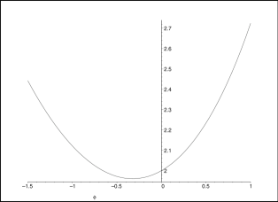
Figure 1: Typical shape of the effective potential $V_{\rm eff}(\phi)$ for the dilaton. The plot is for $\frac{1}{2}\frac{Q^{2}}{\xi^{2}}=1$ and $\frac{T_{6}}{\zeta}=1$.

III.1 Radion stabilization for fixed dilaton

In this subsection, assuming that the dilaton is fixed, we will show that the radion can be stabilized while the volume of the three-dimensional subspace grows indefinitely. When the dialton is localized at its critical value $\phi=\phi_{0}$, we obtain, from (27) and (28),

$$\frac{\ddot{\zeta}}{\zeta}-\frac{4D-9}{2(D-1)}T_{D-3}\frac{e^{\frac{3}{4}\phi_{0}}}{\zeta}=\frac{\ddot{\xi}}{\xi}-\frac{D-6}{D-1}\Lambda-\frac{3(2D-7)}{2(D-1)}Q^{2}\frac{e^{-\frac{1}{2}\phi_{0}}}{\xi^{2}}.$$ (33)

Since the left-hand side is a function of $\zeta$ while the right-hand side is a function of $\xi$, we take the simplest case by equating them to a constant $E$

$$\frac{\ddot{\zeta}}{\zeta}=E+\frac{4D-9}{2(D-1)}T_{D-3}\frac{e^{\frac{3}{4}\phi_{0}}}{\zeta},$$ (34)

$$\frac{\ddot{\xi}}{\xi}=E+\frac{D-6}{D-1}\Lambda+\frac{3(2D-7)}{2(D-1)}Q^{2}\frac{e^{-\frac{1}{2}\phi_{0}}}{\xi^{2}}.$$ (35)

The equations for two volume factors can be written as motions of a particle in one-dimensional potential, ${\ddot{\zeta}}=-\frac{dV_{\rm eff}(\zeta)}{d\zeta}$, ${\ddot{\xi}}=-\frac{dV_{\rm eff}(\xi)}{d\xi}$, where

$$V_{\rm eff}(\zeta) = -\frac{1}{2}E\zeta^{2}-\frac{4D-9}{2(D-1)}e^{\frac{3}{4}\phi_{0}}T_{D-3}\zeta,$$ (36)

$$V_{\rm eff}(\xi) = -\frac{1}{2}(E+\frac{D-6}{D-1}\Lambda)\xi^{2}-\frac{3(2D-7)}{2(D-1)}Q^{2}e^{-\frac{1}{2}\phi_{0}}\ln\xi.$$ (37)

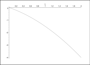
Figure 2: Typical shape of the effective potential $V_{\rm eff}(\zeta)$ for the unwrapped subvolume. The plot is for $E=1$ and $\frac{27}{16}T_{6}e^{\frac{3}{4}\phi_{0}}=1$.

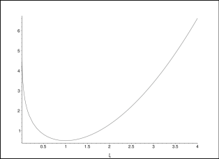
Figure 3: Typical shape of the effective potential $V_{\rm eff}(\xi)$ for the wrapped subvolume for $\Lambda=-|\Lambda|<0$ and $E-\frac{3}{8}|\Lambda|<0$. The plot is for $E-\frac{3}{8}|\Lambda|=-1$ and $\frac{33}{16}Q^{2}e^{\frac{1}{2}\phi_{0}}=1$.

To have a monotonic expansion for $\zeta$, we require the condition $E>0$. In this case the shape of $V_{\rm eff}(\zeta)$ is runaway-type as shown in Fig. 2. The solution for $\zeta$ of Eq. (34) is exponentially increasing $\zeta\sim e^{\sqrt{E}t}$. Thus the three-dimensional volume can grow indefinitely.

For the confining behavior for large $\xi$, we require the condition

$$\Lambda=-|\Lambda|<0,~{}~{}~{}~{}E-\frac{D-6}{D-1}|\Lambda|<0.$$ (38)

Then the shape of the potential $V_{\rm eff}(\xi)$ is well-type as shown in Fig. 3. Substituting $D=9$, the range of the parameter $E$ is $0<E<\frac{3}{8}|\Lambda|$. For parameters satisfying (38) the internal volume can oscillate around the minimum of the potential or sit at the minimum of the potential

$$\xi_{\rm min}=\Bigl{(}\frac{\frac{33}{16}Q^{2}e^{-\frac{1}{2}\phi_{0}}}{\frac{3}{8}|\Lambda|-E}\Bigr{)}^{\frac{1}{2}}.$$ (39)

The idea for the perturbative analysis starts from setting the asymptotic value of the radion equal to its critical value $\xi_{0}=\xi_{\rm min}$. Then we examine what happens when the radion is deviated from this value. Considering the radion perturbation up to first order

$$\xi=\xi_{0}+\delta\xi,$$ (40)

we obtain

$${\ddot{\delta\xi}}=-\Bigl{(}\frac{3}{8}|\Lambda|-E\Bigr{)}\delta\xi-\frac{33}{16}Q^{2}\frac{e^{-\frac{1}{2}\phi_{0}}}{\xi_{0}^{2}}\delta\xi.$$ (41)

Using Eq. (39), the solution is easily obtained as the following form of oscillating solution

$${\delta\xi}=\delta\xi_{0}\sin\omega_{\xi}t,~{}~{}~{}~{}\omega_{\xi}=\sqrt{2\Bigl{(}\frac{3}{8}|\Lambda|-E\Bigr{)}}.$$ (42)

Thus the radion can be stabilized if the dilaton is fixed at its critical value.

III.2 Dilaton stabilization for fixed radion

In this subsection, assuming that the volume factor of the three-dimensional space grows indefinitely $\zeta\sim e^{\sqrt{E}t}$ and the radion is fixed at $\xi_{0}$, we will show that the dilaton can be stabilized. We consider the dilaton perturbation up to first order:

$$\phi=\phi_{0}+\delta\phi.$$ (43)

Then we obtain the following equation for the perturbed field, from Eq. (29),

$${\ddot{\delta\phi}}+\frac{\dot{\zeta}_{0}}{\zeta_{0}}\dot{\delta\phi}+\frac{1}{8}Q^{2}\frac{e^{-\frac{1}{2}\phi_{0}}}{\xi_{0}^{2}}\delta\phi+\frac{9}{16}T_{6}\frac{e^{\frac{3}{4}\phi_{0}}}{\zeta_{0}}\delta\phi=0.$$ (44)

Substituting $\zeta_{0}\sim e^{\sqrt{E}t}$ and using Eq. (32) and Eq. (39), we have

$${\ddot{\delta\phi}}+\sqrt{E}\dot{\delta\phi}+\frac{5}{33}\Bigl{(}\frac{3}{8}|\Lambda|-E\Bigr{)}\delta\phi=0.$$ (45)

The general solution is given by

$$\delta\phi=Ae^{\alpha_{+}t}+Be^{\alpha_{-}t},$$ (46)

where

$$\alpha_{\pm}=\frac{-\sqrt{E}\pm\sqrt{\frac{53}{33}E-\frac{5}{22}|\Lambda|}}{2}.$$ (47)

There are two possible solutions depending on the sign of the discriminant for the parameter range $0<E<\frac{3}{8}|\Lambda|$.

i) for $0<E<\frac{15}{106}|\Lambda|$, $\alpha_{\pm}$ are complex with their real part negative. In this case, $\delta\phi$ can have the following form of the damped oscillation:

$$\delta\phi=\delta\phi_{0}e^{-\frac{\sqrt{E}}{2}t}\sin\omega_{\phi}t,~{}~{}~{}~{}\omega_{\phi}=\frac{1}{2}\sqrt{\frac{5}{22}|\Lambda|-\frac{53}{33}E}.$$ (48)

ii) for $\frac{15}{106}|\Lambda|<E<\frac{3}{8}|\Lambda|$, both $\alpha_{+}$ and $\alpha_{-}$ are negative. In this case, the perturbation is exponentially decreasing.

Thus the dilaton can be stabilized as far as the parameter $E$ is in the range $0<E<\frac{3}{8}|\Lambda|$.

IV Dynamical stabilization

We have seen that both the radion and the dilaton are stabilized separately assuming one of the two is fixed. In this section, we consider the dynamical stabilization when both moduli are perturbed from their critical values. When the sign of the parameter $E$ is positive, the volume of the three-dimensional subspace $\zeta$ will increase indefinitely. Due to this inflation in the three dimensions, terms proportional to $1/\zeta$ can be ignored soon after the onset of this regime. We also ignore the damping term because the presence of this term always contributes to the stabilization positively. We start our perturbative analysis from setting the asymptotic values of the two moduli equal to their critical values. We will examine what happens when the two fields are deviated from their critical values, $\phi=\phi_{0}$ and $\xi=\xi_{0}$.

Substituting

$$\phi=\phi_{0}+\delta\phi,~{}~{}~{}~{}\xi=\xi_{0}+\delta\xi,$$ (49)

and keeping only linear terms in the perturbation, we have the following system of equations for the radion and the dilaton

$${\ddot{\delta\xi}}+\Bigl{(}\frac{3}{8}|\Lambda|-E+\frac{33}{16}Q^{2}\frac{e^{-\frac{1}{2}\phi_{0}}}{\xi_{0}^{2}}\Bigr{)}{\delta\xi}+\frac{33}{32}Q^{2}\frac{e^{-\frac{1}{2}\phi_{0}}}{\xi_{0}}{\delta\phi}=0,$$ (50)

$${\ddot{\delta\phi}}+\frac{1}{2}Q^{2}\frac{e^{-\frac{1}{2}\phi_{0}}}{\xi_{0}^{3}}{\delta\xi}+\frac{1}{8}Q^{2}\frac{e^{-\frac{1}{2}\phi_{0}}}{\xi_{0}^{2}}{\delta\phi}=0.$$ (51)

To find the eigenvalues of the coupled equations, we make the ansatz:

$$\begin{pmatrix}\delta\xi\cr\delta\phi\cr\end{pmatrix}~{}=~{}\begin{pmatrix}\delta\xi_{0}\cr\delta\phi_{0}\cr\end{pmatrix}e^{i\omega t}.$$ (52)

Then the system of equations can be written in matrix form using (39),

$$\begin{pmatrix}-\omega^{2}+2(\frac{3}{8}|\Lambda|-E)&\frac{1}{2}(\frac{3}{8}|\Lambda|-E){\xi_{0}}\cr\frac{8}{33}(\frac{3}{8}|\Lambda|-E)\frac{1}{\xi_{0}}&-\omega^{2}+\frac{2}{33}(\frac{3}{8}|\Lambda|-E)\cr\end{pmatrix}\begin{pmatrix}\delta\xi_{0}\cr\delta\phi_{0}\cr\end{pmatrix}e^{i\omega t}=0.$$ (53)

The eigenvalues of $\omega$ are given by

$$\omega^{2}\Bigl{\{}\omega^{2}-\frac{68}{33}\Bigl{(}\frac{3}{8}|\Lambda|-E\Bigr{)}\Bigr{\}}=0.$$ (54)

The stability condition for the moduli is that $\omega^{2}$ have real and positive roots. The existence of any imaginary part in $\omega$ means that $e^{i\omega t}$ can grow exponentially, which means the instability. Obviously equation (54) satisfies this stability condition and the nontrivial solution of $\omega$ are

$$\omega=\pm\sqrt{\frac{68}{33}\Bigl{(}\frac{3}{8}|\Lambda|-E\Bigr{)}}.$$ (55)

In conclusion, the radion and the dilaton can be stabilized dynamically to their attractor values.

V Conclusions

We have shown that the radion and the dilaton can be stabilized simultaneously. Our derivation is based on the dependence of dilaton, radion, and three-dimensional scale factor on their effective potentials generated by the brane gas and the RR flux. The existence of a $(D-3)$-brane gas wrapping the extra dimensions and a four-form RR flux in the unwrapped dimensions can cause attractor potentials for dilaton and radion. In order to stabilize the moduli, one requires both the negative and the positive sources of forces. The brane gas is the origin of a potential term that can make the radion to contract. The role of the RR flux is to prevent the radion from collapse. It gives a logarithmic bounce for small values of the radion. The dilaton field shows a confining potential consisting of a sum of positive and negative exponential walls originated from the flux and the brane gas.

In general, the two criteria for the stabilization of a scalar field are as follows. First, as a function of scalar field, $V_{\rm eff}(\phi)$ must have a critical point $\frac{\partial}{\partial\phi}V_{\rm eff}(\phi_{0})=0$. Second, the second derivative of the effective potential at the critical point $\frac{\partial^{2}}{\partial\phi^{2}}V_{\rm eff}(\phi_{0})$ must be positive. One can easily check that, from (31) and (37), both conditions are satisfied when one of the moduli is fixed. Since the dilaton field and the radion field are coupled, we perturbed both fields from their critical values and found that they are stable. It is important that the effective potential for the dilaton comes from their coupling to gauge field and brane gas. For any models where the dilaton potential is known in the string theory background, one can check the condition for stability by the above-mentioned criteria in the Einstein frame.

One important point in moduli stabilization is the frame. To study the field equations we worked in the ten-dimensional Einstein frame. One may study the moduli stabilization in four dimensional Einstein frame after dimensionally reducing the ten-dimensional theory to four dimensional theory. For fixed dilaton the two results should be the same. However, when one tries to fix both the dilaton and the radion dynamically, one should work in the ten-dimensional Einstein frame. Analysis based on lower dimensional effective action may be different from the analysis in the original higher dimensional action.

In our calculation, we introduced the cosmological constant without further explanation of its origin. Let us briefly sketch whether it is possible to achieve the stabilization without this term. Neglecting the damping terms, since the damping terms contribute stabilization positively, we consider the time evolution of the differential equation of the form ${\ddot{x}}=kx$. The solution of $x(t)$ is exponential for positive $k$ and oscillating for negative $k$. The initial parameter condition for the inflation of three-dimensional scale factor and stabilization of dilaton and radion can be obtained from Eqs (22), (23), and (24), for $D=9$,

$$T_{6}\frac{e^{\frac{3}{4}\phi}}{a^{3}}>3Q^{2}\frac{e^{-\frac{1}{2}\phi}}{b^{12}}.$$ (56)

Naively it seem that our stabilization argument can be applied to the cases without cosmological constant term for some initial values of the moduli. More studies regarding the cosmological constant are needed.

- (1) E. Silverstein, hep-th/0405068; L. McAllister and E. Silverstein, Gen. Rel. Grav. 40, 565 (2008).
- (2) R. Brandenberger and C. Vafa, Nucl. Phys. B 316, 391 (1989); A. A. Tseytlin and C. Vafa, Nucl. Phys. B 372, 443 (1992); A. A. Tseytlin, Class. Quant. Grav. 9, 979 (1992).
- (3) S. Alexander, R. Brandenberger, and D. Easson, Phys. Rev. D 62, 103509 (2000).
- (4) S. Watson and R. Brandenberger, J. Cocmol. Astropart. Phys. 0311, 008 (2003).
- (5) S. P. Patil and R. Brandenberger, Phys. Rev. D 71, 103522 (2005); J. Cocmol. Astropart. Phys. 0601, 005 (2006).
- (6) T. Battefeld and S. Watson, J. Cocmol. Astropart. Phys. 0406, 001 (2004).
- (7) S. Watson, Phys. Rev. D 70, 066005 (2004).
- (8) Y-K. E. Cheung, S. Watson, and R. Brandenberger, J. High Energy Phys. 0605, 025 (2006).
- (9) A. Campos, Phys. Rev. D 71, 083510 (2005).
- (10) T. Rador, Eur. Phys. J. C 49, 1083 (2007).
- (11) S. P. Patil, hep-th/0504145.
- (12) A. Kaya, Phys. Rev. D 72, 066006 (2005).
- (13) D. A. Easson and M. Trodden, Phys. Rev. D 72, 026002 (2005).
- (14) A. Chatrabhuti, Int. J. Mod. Phys. A 22, 165 (2007).
- (15) J. Y. Kim, Phys. Lett. B 652, 43 (2007).
- (16) S. Arapoglu, A. Karakci, and A. Kaya, Phys. Lett. B 645, 255 (2007).
- (17) J. Y. Kim, Phys. Rev. D 78, 066003 (2008).
- (18) A. J. Berndsen and J. M. Cline, Int. J. Mod. Phys. A 19, 5311 (2004).
- (19) A. Berndsen, T. Biswas, and J. M. Cline, J. Cocmol. Astropart. Phys. 0508, 012 (2005).
- (20) T. Biswas, R. Brandenberger, D. A. Easson, and A. Mazumdar, Phys. Rev. D 71, 083514 (2005).
- (21) S. Kanno and J. Soda, Phys. Rev. D 72, 104023 (2005).
- (22) S. Cremonini and S. Watson, Phys. Rev. D 73, 086007 (2006).
- (23) T. Rador, Eur. Phys. J. C 52, 683 (2007).
- (24) M. Sano and H. Suzuki, Phys. Rev. D 78, 064045 (2008); arXiv:0907.2495 [hep-th].
- (25) R. J. Danos, A. R. Frey, and R. H. Brandenberger, Phys. Rev. D 77, 126009 (2008).
- (26) K. Dasgupta, G. Rejesh, and S. Sethi, J. High Energy Phys. 9908, 023 (1999).
- (27) S. B. Giddings, S. Kachru, and J. Polchinski, Phys. Rev. D 66,106006 (2002).
- (28) W. D. Goldberger and M. B. Wise, Phys. Rev. Lett. 83, 4922 (1999).