Generalized Parton Distributions for the Proton in Position Space : Zero Skewness

Abstract

We present a study of the parton distributions in transverse position or impact parameter space using a recent parametrization of u and d quark generalized parton distributions (GPDs) $H(x,t)$ and $E(x,t)$ at zero skewness. We make a comparative study between different parametrizations and discuss the region of validity of the positivity condition.

Introduction

Generalized parton distributions (GPDs) contain a wealth of information about the nucleon structure (see rev for example). Unlike the ordinary parton distributions (pdfs) which at a given scale depend only on the longitudinal momentum fraction $x$ of the parton, GPDs are functions of three variables, $x$, $\zeta$ and $t$ where the so-called skewness $\zeta$ gives the longitudinal momentum transfer and $-t$ is the square of the momentum transfer in the process. These are called off-forward parton distributions. The GPDs give interesting information about the spin and orbital angular momentum of the quarks and gluons in the nucleon as well as their spatial distribution. They are experimentally accessed through the overlap of deeply virtual Compton scattering (DVCS) and Bethe-Heitler (BH) process as well as exclusive vector meson production rev . Data has been obtained at HERA collider, by the H1 H1 ; H2 and ZEUS ZEUS1 ; ZEUS2 collaborations and HERMES HERMES fixed target experiment. DVCS experiments are also being done at JLAB Hall A and B CLAS . COMPASS at CERN has programs to access GPDs through muon beams COMPASS . Experimental observables, however involve a convolution of GPDs, and so modeling GPDs is interesting. GPDs reduce to ordinary forward parton distributions (pdfs) in the forward limit. Moments over $x$ give nucleon form factors. These act as useful constraints to model the GPDs. A large number of models or parametrizations have been proposed for GPDs. Here we do not plan to review all of them but mention only those that are relevant for us. A detailed list of the main lines of approach and their present status with respect to the data can be found in boffi . Moments of GPDs have been calculated on lattice as well. In marc , GPDs at zero skewness $\zeta$ have been parametrized in a Regge type model at small $x$ and using a modified Regge parametrization at large $x$ and $t$. It was found to describe the basic features of proton and neutron electromagnetic form factors. Similar small $x$ Regge type behaviour was used in the modeling of pion GPDs in rad . Another parametrization of GPDs at zero skewness is given in diehl . Here a Regge motivated $x$ dependence at small $x$ was interpolated to large $x$ region. The GPDs at the input scale were fitted to the experimental data on Dirac and Pauli form factors. An exponential $t$ dependence was used. The form of the $t$ dependence was found to be unchanged by the scale evolution. In liuti a recent parametrization was proposed for zero skewness and an extension to non-zero $\zeta$ was done in l2 . At the input scale the GPDs were parametrized by a spectator model term multiplied by a Regge motivated term. The parameters were obtained by fitting the forward pdfs and form factors.

For non-zero $\zeta$, the GPDs have to satisfy an additional constraint, namely polynomiality. In certain models, for example using the overlap of light-front wave functions (LFWFs), it is very difficult to obtain a suitable parametrization of the higher Fock components of the wave function in order to get the polynomiality of GPDs. Polynomiality is satisfied by construction only if one considers the LFWFs of simple spin $1/2$ objects like a dressed quark or a dressed electron in perturbation theory instead of the proton overlap ; us . A recent fit to the DVCS data at small Bjorken $x$ from H1 and ZEUS was done in dieter , using the conformal Mellin-Barnes representation of the DVCS amplitude. However, to get the GPDs one has to do an inverse Mellin transform, and a knowledge of all moments are required for that.

At zero skewness $\zeta$, if one performs a Fourier transform (FT) of the GPDs with respect to the momentum transfer in the transverse direction $\Delta_{\perp}$, one gets the so called impact parameter dependent parton distributions (ipdpdfs), which gives how the partons of a given longitudinal momentum are distributed in transverse position (or impact parameter $b_{\perp}$) space. These obey certain positivity constraints and unlike the GPDs themselves, have probabilistic interpretation burkardt . These give an interesting interpretation of Ji’s angular momentum sum rule ji . Due to rotational invariance, the same relation should hold for all components of the angular momentum $\vec{J_{q}}$. In the impact parameter space, the relation for $J^{\perp}_{q}$ has a simple partonic interpretation for transversely polarized state bur05 ; the term containing $E(x,0,0)$ arises due to a transverse deformation of the GPDs in the center of momentum frame. The term containing $H(x,0,0)$ is an overall transverse shift when going from the transversely polarized state in instant form (rest frame) to the front form (infinite momentum frame). On the other hand, in hadron_optics , real and imaginary parts of the DVCS amplitudes are expressed in longitudinal position space by introducing a longitudinal impact parameter $\sigma$ conjugate to the skewness $\zeta$, and it was shown that the DVCS amplitude show certain diffraction pattern in the longitudinal position space. Since Lorentz boosts are kinematical in the front form, the correlation determined in the three-dimensional $b_{\perp},\sigma$ space is frame-independent. As GPDs depend on a sharp $x$, the Heisenberg uncertainty relation restricts the longitudinal position space interpretation of GPDs themselves. It has, however, been shown in wigner that one can define a quantum mechanical Wigner distribution for the relativistic quarks and gluons inside the proton. Integrating over $k^{-}$ and $k^{\perp}$, one obtains a four dimensional quantum distribution which is a function of ${\vec{r}}$ and $k^{+}$ where ${\vec{r}}$ is the quark phase space position defined in the rest frame of the proton. These distributions are related to the FT of GPDs in the same frame. This gives a 3D position space picture of the GPDs and of the proton.

In this series of work, we plan to investigate the GPDs for the proton in transverse and longitudinal position space. In this first paper, we study the recently parametrized form in liuti in impact parameter space and make a comparative study with other models.

Parametrization of the GPDs

We consider the parametrization in liuti for the GPDs :

Set I

$$H^{I}(x,t) = G_{M_{x}^{I}}^{\lambda^{I}}(x,t)\,x^{-\alpha^{I}-\beta_{1}^{I}(1-x)^{p_{1}^{I}}t}$$ (1)

$$E^{I}(x,t) = \kappa\,G_{M_{x}^{I}}^{\lambda^{I}}(x,t)\,x^{-\alpha^{I}-\beta_{2}^{I}(1-x)^{p_{2}^{I}}t}$$ (2)

Set II

$$H^{II}(x,t) = G_{M_{x}^{II}}^{\lambda^{II}}(x,t)\,x^{-\alpha^{II}-\beta_{1}^{II}(1-x)^{p_{1}^{II}}t}$$ (3)

$$E^{II}(x,t) = G_{\widetilde{M}_{x}^{II}}^{\widetilde{\lambda}^{II}}(x,t)\,x^{-\widetilde{\alpha}^{II}-\beta_{2}^{II}(1-x)^{p_{2}^{II}}t}$$ (4)

All parameters except for $p_{1}$ and $p_{2}$ are flavor dependent. The function $G$ has the same form for both parametrizations, I and II:

$$G_{M_{x}}^{\lambda}(x,t)= {\cal N}\frac{x}{1-x}\int d^{2}{\bf k}_{\perp}\frac{\phi(k^{2},\lambda)}{D(x,{\bf k}_{\perp})}\frac{\phi({k^{\prime\,2},\lambda)}}{D(x,{\bf k}_{\perp}+(1-x){\bf\Delta}_{\perp})},$$ (5)

where

$$D(x,{\bf k}_{\perp})\equiv k^{2}-m^{2},$$ (6)

$$k^{2} = xM^{2}-\frac{x}{1-x}M_{x}^{2}-\frac{{\bf k}_{\perp}^{2}}{1-x}$$ (7)

$$k^{\prime\,2} = xM^{2}-\frac{x}{1-x}M_{x}^{2}-\frac{({\bf k}_{\perp}-(1-x)\Delta)^{2}}{1-x},$$ (8)

and

$$\phi(k^{2},\lambda)=\frac{k^{2}-m^{2}}{|k^{2}-\lambda^{2}|^{2}},$$ (9)

Here $\zeta$, the skewness variable is taken to be zero, in other words, momentum transfer is in the transverse direction. $t$ is the invariant momentum transfer squared, $t=-\Delta^{2}$, and $x$ is the fraction of the light cone momentum carried by the active quark, $k$ being its momentum. The mass parameters are $m$, the struck quark mass, and $M$, the proton mass. The normalization factor includes the nucleon-quark-diquark coupling, and it is set to ${\cal N}=1$ GeV⁶.

The $u$ and $d$ quark contributions to the anomalous magnetic moments are:

$$\kappa\equiv\kappa^{q}=\left\{\begin{array}[]{ll}\kappa^{d}=-2.03,&\;{\rm for}\;q=d\\ \kappa^{u}/2=1.67/2,&\;{\rm for}\;q=u\end{array}\right..$$ (10)

The parameters are listed in liuti for both the sets. The parameters $M_{x}^{q}$, $\lambda^{q}$ and $\alpha^{q}$, $q=u,d$, obtained at an initial scale $Q_{0}^{2}$ ($Q^{2}_{0}=0.094$ GeV²), and they are the same for both Sets I and II, in Set I they are by definition the same for the functions $H$ and $E$ (see Eqs. (1,2)). The parameters in this model are obtained by fitting the experimental data on the nucleon electric and magnetic form factors (see liuti for reference). For the forward limit, Alekhin ale leading order (LO) pdf sets were fitted within the range $10^{-5}\leq x\leq 0.8$ and $4\leq Q^{2}\leq 240~{}\mathrm{GeV}^{2}$ by valence distribution and using the baryon number and momentum sum rules. The input scale $Q_{0}^{2}=0.094~{}\mathrm{GeV}^{2}$ is obtained as a parameter in this model. The low value of $Q_{0}^{2}$ results from the requirement that only valence quarks contribute in the momentum sum rule.

The above phenomenologically motivated parametrization of the GPDs $H(x,t)$ and $E(x,t)$ at zero skewness $\zeta$ was done using a spectator model calculation at the low input scale. The spectator model has been used for its simplicity and for the fact that it is flexible enough to predict the main features of a number of distribution and fragmentation functions in the intermediate and large $x$ region. The spectator mass is chosen to be different for different quark flavor GPDs. However, similar to the case of pdfs, the spectator model is not able to reproduce quantitatively the small $x$ behaviour of the GPDs. So a ‘Regge-type’ term has been considered multiplying the spectator model function $G_{M_{x}}^{\lambda}$. The parameters were obtained by fitting the form factors and forward pdfs. Two versions of the parametrizations were used and are given by set I and set II. The GPD $E$ is unconstrained by the data on forward pdfs, so in set II an additional normalization condition has been imposed

$$\int_{0}^{1}dxE_{q}(x,t=0)=\kappa^{q}$$ (11)

with the experimental values of $\kappa^{u}$ and $\kappa^{d}$.

Although $H^{u}$ and $H^{d}$ are similar in behaviour in both sets of parametrization, the main difference is in the behaviour of $E^{u}$ and $E^{d}$ (see Fig. 9 of liuti ) at the input scale. $E^{u}$ is a slowly increasing function of $x$ for set I, and for set II, it increases rapidly as $x$ approaches zero. $E_{d}$ has a peak at larger value of $x$ for set II. It was found that the difference between the sets decreases if one evolves the GPDs to higher values of $Q^{2}$ (scale). It is to be noted that the parametrizations for marc and diehl are at different input scales compared to liuti . However the GPDs are evolved to the respective scales of marc and diehl and a comparison is provided in Figs. (13-16) of liuti . For $H^{u}$ and $H^{d}$ although there is agreement for low $-t$, for higher $-t$ the results differ qualitatively and quantitatively. For $E^{u}$ and $E^{d}$ the disagreement is also at lower $-t$.

Again, even at $Q^{2}=4~{}\mathrm{GeV}^{2}$, there is significant difference between set I and set II. $H^{u}$ and $H^{d}$ agrees with lattice calculations of lattice at $t=-0.3~{}\mathrm{GeV}^{2}$, but the qualitative behaviour is different and even is outside the error band of lattice calculations for higher values of $\mid t\mid$.

Parton distributions in impact parameter space

Parton distribution in impact parameter space $q(x,b)$ is defined as burkardt :

$$q(x,b)={1\over 4\pi^{2}}\int d^{2}\Delta e^{-i\Delta^{\perp}\cdot b^{\perp}}H(x,t)$$

$$e(x,b)={1\over 4\pi^{2}}\int d^{2}\Delta e^{-i\Delta^{\perp}\cdot b^{\perp}}E(x,t).$$ (12)

These functions have the physical interpretation of measuring the probability to find a quark of longitudinal momentum fraction $x$ at a transverse position $b_{\perp}$ in the nucleon. Here $b=\mid b_{\perp}\mid$ is the impact parameter which is the transverse distance between the struck parton and the center of momentum of the hadron. $b$ is defined such a way that $\sum_{i}x_{i}b_{i}=0$ where the sum is over the number of partons. The relative distance ${b\over 1-x}$ between the struck parton and the spectator system provides an estimate of the size of the system as a whole.

In Fig. 1-2 we have plotted $q(x,b)$ and $e(x,b)$, both for u and d quarks and for set I. The values of the parameters used are from liuti at the input scale. For small and medium $x$, $e^{d}(x,b)$ is larger in magnitude than $e^{u}(x,b)$. The peak shifts to higher $x$ as $b$ decreases. This means that the $d$ quark dominates in the proton helicity flip distribution. However, $u$ quark contribution dominates in the helicity non-flip $q(x,b)$. $e^{d}$ is negative whereas $e^{u}$ is positive, similar to the model in marc . However, in the model we study, $e^{d}(x,b)$ is comparable with or even larger in magnitude than $q^{d}(x,b)$, unlike in marc , where it is much smaller at the input scale. In the parametrization of marc , the $t$ dependence is only in the argument of the exponential and the Fourier transform is simpler and can be obtained analyically. The resulting parton distributions in the impact parameter space are larger in magnitude than what we get in this work using the parametrization of liuti which may be due to the different scale $Q_{0}^{2}$ in the plots. In diehl , $2-D$ distributions in the $b_{x}-b_{y}$ plane are plotted. The smearing of the quark distributions in the transverse impact parameter plane decreases as $x$ increases, which means that the parton distributions are more localized for higher values of $x$. Similar behaviour is observed in the model of marc . As $x$ approaches $1$, the transverse width of $q(x,b)$ should vanish burkardt . In this limit $q(x,b)$ should have a very peaked transverse profile, as $H(x,t)$ is independent of $t$ when $x\rightarrow 1$ as the active quark carries all the proton momentum no matter what $t$ is. However, from Fig. 1 we see that as $x\rightarrow 1$, the peak of the distribution decreases.

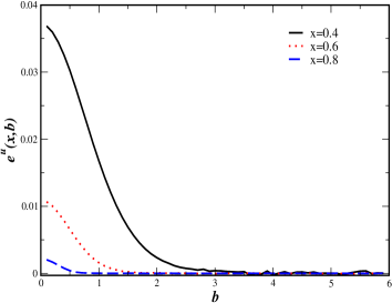
(a)   (b)

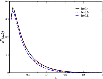
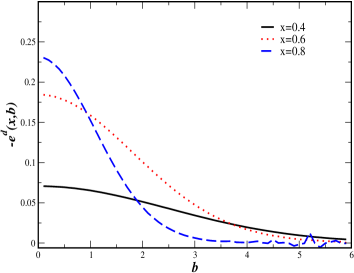
(c)   (d)

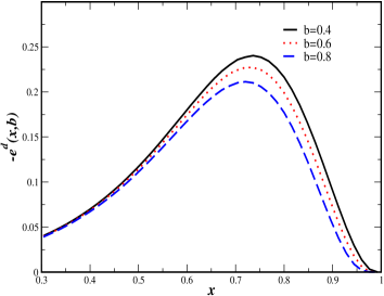
Figure 3: (Color online) Plots of (a) $e^{u}(x,b)$ vs $b=\mid b_{\perp}\mid$ for fixed values of $x$, (b) $e^{u}(x,b)$ vs $x$ for fixed values of $b$, (c) same as in (a) but for $-e^{d}$, (d) same as in (b) but for $-e^{d}$. Parameters are as in set II. $b$ is in $\mathrm{GeV}^{-1}$.

$q(x,b)$ both for u and d quarks in set II are the same as in set I. In Figs. 3, we have plotted $e(x,b)$ for u and d quarks where the parameters are as in set II. $e(x,b)$ has a different behaviour compared to set I. The peak of $e^{u}$ is shifted to very small value of $x$ and $e^{u}(x,b)$ decreases sharply as $x$ increases. That means at larger $x$, d quark dominates in $e(x,b)$.

The Fourier transform of the GPD $E(x,t)$ plays an important role when instead of an unpolarized target we have a transversely polarized target. In other words, it has a probability interpretation in the transversity basis rather than the helicity basis. For a state polarized in the x direction, parton distribution in the impact parameter space becomes burkardt

$$q^{X}(x,b)=q(x,b)-{1\over 2M}{\partial e(x,b)\over\partial b_{y}}$$ (13)

This means that the GPD $E(x,t)$ causes a transverse shift of the quark distribution in a transversely polarized target. For a state polarized in x direction the shift is in the y direction and so on. The magnitude of the shift is given by ${1\over 2M}\mid{\partial e(x,b)\over\partial b_{y}}\mid$. The average displacement of the shift is given by

$${{\langle b^{y}\rangle}^{q}}_{X}={\int d^{2}bb^{y}q^{X}(x,b)\over\int d^{2}bq^{X}(x,b)}={1\over 2M}{E^{q}(x,0)\over H^{q}(x,0)}.$$ (14)

The distance between the struck quark and the spectator system is given by

$$s^{q}(x)={{<b^{y}>}^{q}_{X}\over 1-x}$$ (15)

For $d$ quarks, $s^{q}(x)$ is larger in magnitude than $u$ diehl . The transverse shift depends on the set of parameters used in the model considered here liuti .

The parton distributions in impact parameter space should obey the positivity condition burkardt2

$$q(x,b)\geq{1\over 2M}\mid{\partial e(x,b)\over\partial b_{i}}\mid.$$ (16)

This follows from the fact that $q^{X}(x,b)$ which is the unpolarized parton distribution for transversely polarized proton should have probability interpretation.

The positivity relation in effect puts an upper bound on $b$. In the model of marc , it was found that for u quarks, the positivity bound was satisfied over most of the $x$ region, considering that the GPDs are vanishingly small for values of $b$ larger than the nucleon size. For d quarks, a violation of positivity was observed which is more pronounced at larger values of $x$ and $b$. However the violation is small. In the model of diehl , the positivity condition was used to constrain the behaviour of $E(x,t=0)$ at large values of $x$. In Fig. 4 we have plotted $q(x,b)$ as well as ${1\over 2M}\mid{\partial e(x,b)\over\partial b}\mid$ for u and d quarks for both the parametrizations in liuti , as functions of $b$. We see that in set I for u quarks, positivity is mildly violated for very large values of $x$ and for $b>0.5~{}\mathrm{GeV}^{-1}$. For u quarks in set II there is no violation. For d quarks in set I, positivity is not violated for any $b$ values for $x<0.1$. It is violated at larger $b$ values or comparatively larger $x$. Violation is more as $x$ increases. For d quarks in set II, positivity is largely violated for large $x,b$ values. To see the $x$ dependence of the violation of positivity, in Fig. 5 we plot the same quantities as in Fig. 4, as functions of $x$, for fixed values of $b$. For u quarks in set I positivity is violated for $b\approx 0.4~{}\mathrm{GeV}^{-1}$ for large values of $x$. For higher $b$ values, violation is even at smaller values of $x$. Violation of positivity is not seen in u quarks in set II. For d quraks in set I, there is larger violation of positivity and it starts already at $x=0.2$ for large $b$. For d quarks in set II there is again a large violation of positivity that starts at $x\approx 0.3$ for $b=5~{}\mathrm{GeV}^{-1}$.

Conclusion

In this paper, we have studied the GPDs $H(x,t)$ and $E(x,t)$ for zero skewness in a recently parametrized form liuti in transverse position or impact parameter space. We present a comparative study between several models. A violation of the positivity condition was observed in certain range of $x,b$. This puts additional constraint on the kinematical region where this parametrization is to be used. This depends on the set of parameters used in the model. A new fit of the parameters with this additional constraint may improve the model. As extension to nonzero $\zeta$ was proposed in l2 . In a future work, we plan to investigate the GPDs with nonzero skewness both in transverse and longitudinal position spaces. In particular, a study in longitudinal position space is interesting to understand the origin of the observed diffraction pattern in the DVCS amplitude in a simple QED model hadron_optics .

Ackowledgement: AM thanks DST fasttrack scheme, Govt. of India, for support. We thank S. Liuti and S. Ahmad for helpful communication.

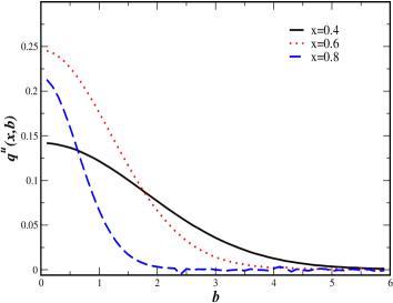
(a)    (b)

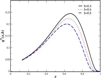
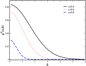
(c)   (d)

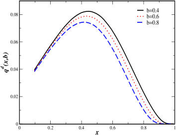
Figure 1: (Color online) Plots of (a) $q^{u}(x,b)$ vs $b=\mid b_{\perp}\mid$ for fixed values of $x$, (b) $q^{u}(x,b)$ vs $x$ for fixed values of $b$, (c) same as in (a) but for $q^{d}$, (d) same as in (b) but for $q^{d}$. Parameters are as in set I. $b$ is in $\mathrm{GeV}^{-1}$.

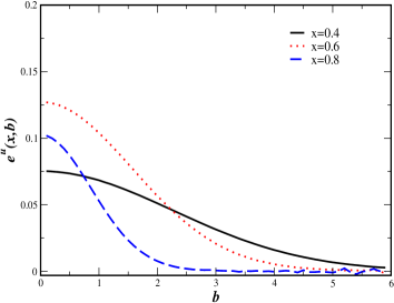
(a)    (b)

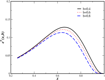
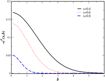
(c)   (d)

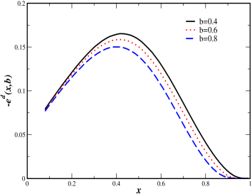
Figure 2: (Color online) Plots of (a) $e^{u}(x,b)$ vs $b=\mid b_{\perp}\mid$ for fixed values of $x$, (b) $e^{u}(x,b)$ vs $x$ for fixed values of $b$, (c) same as in (a) but for $-e^{d}$, (d) same as in (b) but for $-e^{d}$. Parameters are as in set I. $b$ is in $\mathrm{GeV}^{-1}$.

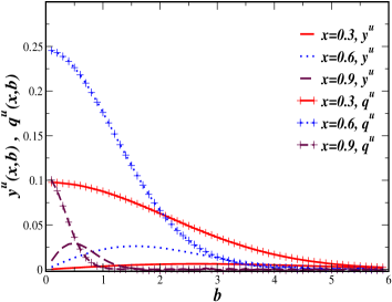
(a)   (b)

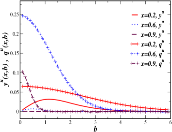
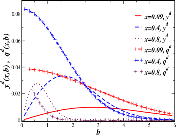
(c)   (d)

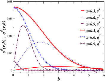
Figure 4: (Color online) Plots of (a) $q^{u}(x,b)$ and $y^{u}(x,b)={1\over 2M}\mid{\partial e^{u}(x,b)\over\partial b}\mid$ vs. $b$ for set I, (b) the same as in (a) but for set II, (c) $q^{d}(x,b)$ and $y^{d}(x,b)={1\over 2M}\mid{\partial e^{d}(x,b)\over\partial b}\mid$ vs. $b$ for set I, (d) the same as in (c) but for set II. $b$ is in $\mathrm{GeV}^{-1}$.

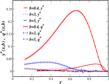
(a)   (b)

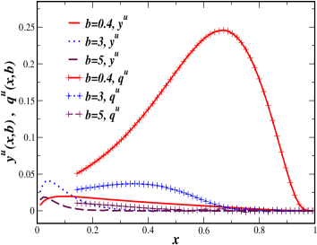
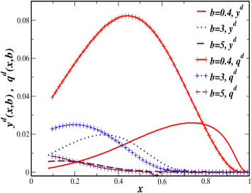
(c)   (d)

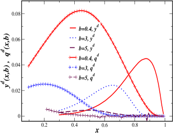
Figure 5: (Color online) Plots of (a) $q^{u}(x,b)$ and $y^{u}(x,b)={1\over 2M}\mid{\partial e^{u}(x,b)\over\partial b}\mid$ vs. $x$ for set I, (b) the same as in (a) but for set II, (c) $q^{d}(x,b)$ and $y^{d}(x,b)={1\over 2M}\mid{\partial e^{d}(x,b)\over\partial b}\mid$ vs. $x$ for set I, (d) the same as in (c) but for set II. $b$ is in $\mathrm{GeV}^{-1}$.

References

- (1) For reviews on generalized parton distributions, and DVCS, see M. Diehl, Phys. Rept, 388, 41 (2003); A. V. Belitsky and A. V. Radyushkin, Phys. Rept. 418 1, (2005); K. Goeke, M. V. Polyakov, M. Vanderhaeghen, Prog. Part. Nucl. Phys. 47, 401 (2001).
- (2) C. Adloff et. al., (H1 Collaboration), Eur. Phys. J. C 13, 371 (2000).
- (3) C. Adloff et. al. (H1 Collaboration), Phys. Lett. B 517, 47 (2001).
- (4) J. Breitweg et. al. (ZEUS Collaboration), Eur. Phy. J. C 6, 603 (1999).
- (5) S. Chekanov et. al. (ZEUS Collaboration), Phys. Lett. B 573, 46 (2003).
- (6) A. Airapetian et. al. (HERMES Collaboration), Phys. Rev. Lett. 87, 182001 (2001).
- (7) S. Stepanyan et. al. (CLAS Collaboration), Phys. Rev. Lett. 87, 182002 (2001).
- (8) N. D’Hose, E. Burtin, P. A. M. Guichon, J. Marroncle (COMPASS Collaboration), Eur. Phys. J. A 19, 47 (2004).
- (9) S. Boffi, B. Pasquini, Riv.Nuovo Cim.30:387,2007.
- (10) M. Guidal, M. V. Polyakov, A. V. Radyushkin, M. Vanderhaeghen, Phys. Rev. D 72, 054013 (2005).
- (11) A. Mukherjee, I. V. Musatov, H. C. Pauli, A. V. Radyushkin, Phys. Rev. D 67, 073014 (2003).
- (12) M. Diehl, T. Feldman, R. Jacob, P. Kroll, Eur. Phys. J. C 39, 1 (2005).
- (13) S. Ahmad, H. Honkanen, S. Liuti and S. Taneja, Phys. Rev. D 75, 094003 (2007).
- (14) S. Ahmad, H. Honkanen, S. Liuti, S. Taneja, arXiv:0708.0268 [hep-ph].
- (15) S. J. Brodsky, M. Diehl, D. S. Hwang, Nucl. Phys. B 596, 99 (2001).
- (16) D. Chakrabarti and A. Mukherjee, Phys. Rev. D 71, 014038 (2005); Phys. Rev. D 72, 034013 (2005); A. Mukherjee and M. Vanderhaeghen, Phys. Lett. B 542, 245; Phys. Rev. D 67, 085020 (2003); D. Chakrabarti, R. Manohar and A. Mukherjee, Phys. Rev. D 79, 034006 (2009).
- (17) K. Kumericki, D. Muller, arXiv:0904.0458 [hep-ph].
- (18) M. Burkardt, Int. J. Mod. Phys. A 18, 173 (2003); M. Burkardt, Phys. Rev. D 62, 071503 (2000), Erratum- ibid, D 66, 119903 (2002); J. P. Ralston and B. Pire, Phys. Rev. D 66, 111501 (2002).
- (19) X. Ji. Phys. Rev. Lett. 78, 610 (1997).
- (20) M. Burkardt, Phys. Rev. D 72, 094020 (2005).
- (21) S. J. Brodsky, D. Chakrabarti, A. Harindranath, A. Mukherjee and J. P. Vary, Phys. Lett. B 641, 440 (2006); Phys. Rev. D 75, 014003 (2007).
- (22) X. Ji, Phy. Rev. Lett. 91, 062001 (2003); A. Belitsky, X. Ji, F. Yuan, Phys. Rev. D 69 074014 (2006).
- (23) S. Alekhin, Phys. Rev. D 68, 014002 (2003).
- (24) G. Schierholz, in GPD 2006: Workshop on Generalized Parton Distributions, June 2006, ECT Trento, Italy.
- (25) M. Burkardt, Phys. Lett. B 582, 151 (2004).
(a) (b)
(b)
(c) (d)
(d)
(a) (b)
(b)
(c) (d)
(d)
(a) (b)
(b)
(c) (d)
(d)
(a) (b)
(b)
(c) (d)
(d)
(a) (b)
(b)
(c) (d)
(d)