Aligned dipolar Bose-Einstein condensate in a double-well potential: From cigar-shaped to pancake-shaped

Abstract

We consider a Bose-Einstein condensate (BEC), which is characterized by long-range and anisotropic dipole-dipole interactions and vanishing $s$-wave scattering length, in a double-well potential. The properties of this system are investigated as functions of the height of the barrier that splits the harmonic trap into two halves, the number of particles (or dipole-dipole strength) and the aspect ratio $\lambda$, which is defined as the ratio between the axial and longitudinal trapping frequencies $\omega_{z}$ and $\omega_{\rho}$. The phase diagram is determined by analyzing the stationary mean-field solutions. Three distinct regions are found: a region where the energetically lowest lying stationary solution is symmetric, a region where the energetically lowest lying stationary solution is located asymmetrically in one of the wells, and a region where the system is mechanically unstable. For sufficiently large aspect ratio $\lambda$ and sufficiently high barrier height, the system consists of two connected quasi-two-dimensional sheets with density profiles whose maxima are located either at $\rho=0$ or away from $\rho=0$. The stability of the stationary solutions is investigated by analyzing the Bogoliubov de Gennes excitation spectrum and the dynamical response to small perturbations. These studies reveal unique oscillation frequencies and distinct collapse mechanisms. The results derived within the mean-field framework are complemented by an analysis based on a two-mode model.

I Introduction

Dipolar BECs have recently attracted a lot of attention both theoretically and experimentally bara08 ; laha08a . The experimental realization of a Cr BEC just a few years ago constitutes an important milestone grie05 . Compared to alkali atoms, Cr has a comparatively large magnetic dipole moment of $6\mu_{B}$, which leads to an enhancement of the dipole-dipole interactions by a factor of 36 compared to alkali atoms. The anisotropy of the dipole-dipole interactions has been observed experimentally by analyzing time of flight expansion images of Cr BECs released from a cylindrically symmetric external confining potential stuh05 . If combined with theoretical calculations, the time of flight images reveal the initial density distribution of the dipolar gas and depend, e.g., on whether the magnetic dipole moments are aligned along the axial or longitudinal confining directions, respectively. Furthermore, by taking advantage of the tunability of the $s$-wave scattering length near a magnetic Fano-Feshbach resonance, the relative importance of the dipole-dipole interactions can be changed wern05 ; koch08 ; laha08 , paving the way for a variety of interesting experimental studies. Dipolar BECs are characterized by intriguing collapse mechanisms sant00 ; yi00 ; yi01 ; gora02 ; eber05 ; bort06 ; fisc06 ; rone07 ; dutt07 ; laha08 ; koch08 ; metz09 , and unique excitation spectra giov02 ; sant03 ; rone07 and vortex structures coop05 ; zhan05 ; yi06 ; odel07 ; wils09 . In addition, dipolar gases loaded into optical lattices may allow for the realization of novel phases gora02a ; dams03 ; meno07 .

Although the dipole-dipole interactions in alkali gases are too weak to result in observable effects in most experiments, it is believed that they play a decisive role in the formation of spin textures in ⁸⁷Rb condensates sadl06 ; veng08 , in the dynamics of Bloch oscillations of ³⁹K BECs loaded into an optical lattice fatt08 and in ⁷Li BECs poll09 . Furthermore, BECs and degenerate Fermi gases that consist of polar molecules may be realized in the near future ni08 ; deig08 ; danz08 . This prospect adds a new intriguing twist since the interactions between two polar molecules can be tuned by an external electric field mari98 . This opens the possibility to enter the strongly-correlated regime and thus to realize a variety of condensed matter analogs gora02a ; lewe07 ; bloc08 .

This paper considers an aligned dipolar BEC in a double well geometry. Double well potentials play an important role in chemical and condensed matter physics, among other areas. In the context of cold atom physics, $s$-wave dominated alkali systems in a double-well have, e.g., been used to study Josephson-type oscillations aubr96 ; smer97 ; ande98a ; ragh99 ; giov00a ; cata01 ; albi05 ; anan06 ; gati07 . The density oscillations of the Bose gas can be interpreted as corresponding to the charge current that characterizes “standard” condensed matter Josephson junctions. Related to this, the macroscopic quantum self-trapping of atoms in one of the wells has been demonstrated experimentally and has been interpreted within a two-mode model that can be derived from the Gross-Pitaevskii (GP) equation albi05 ; anan06 . The double well system has also been used to experimentally study spin-squeezing este08 . In this context, the left and the right wells of the system serve as the two arms of an interferometer shin04 . The number difference and relative phase of the double well system are conjugate variables, whose combined measurements has revealed that the system is entangled este08 .

Here, we investigate the behaviors of aligned dipoles under cylindrically symmetric harmonic confinement with a repulsive Gaussian potential centered at $z=0$. We limit ourselves to situations where the dipoles are aligned along one of the symmetry axis of the external harmonic confining potential. This restriction reduces the parameter space and also significantly reduces the numerical efforts. Arguably, it may be the conceptually simplest case. We are particularly interested in determining the phase or stability diagram for both cigar-shaped and pancake-shaped harmonic confinement. The boundaries of these phase diagrams are governed by the non-trivial interplay of the dipole-dipole interactions, the energy due to the external harmonic confinement, the energy due to the Gaussian potential and the kinetic energy. The interplay of these energy contributions leads to density profiles unique to anisotropic interactions. In agreement with Ref. xion09 , we observe Josephson oscillations as well as macroscopic quantum self-trapping of the system for appropriately chosen parameters. We characterize the transition between these two regimes by analyzing the excitation spectrum and the real time response of the system to a small perturbation. Our study of two neighboring pancake-shaped dipolar gases can be viewed as a first step towards understanding a multi-layer system of dipolar pancakes. For a single pancake, an angular roton instability has been predicted to occur rone07 . For a layer of two-dimensional dipolar BECs, a new length scale is given by the interlayer distance and the roton instability has been predicted to be enhanced compared to the single layer case wang08 . Other multi-layer studies can be found in Refs. klaw09 ; kobe09 .

The remainder of this paper is organized as follows. Section II introduces the mean-field GP equation and discusses how we determine the stationary and time-dependent solutions. The Bogoliubov de Gennes equations that are employed to determine the excitation spectrum of the dipolar gas are introduced. Section III reviews the two-mode model which provides an intuitive understanding of the time-independent and time-dependent GP solutions in the small $\lambda$ regime. Section IV presents our stationary solutions. We discuss the phase diagram as functions of the number of particles (or equivalently, the mean-field strength), the aspect ratio and, in selected cases, the barrier height. Section V presents our time-dependent studies. We investigate certain dynamically stable regimes and deduce distinct collapse mechanisms from the response of the system to a small perturbation. In addition, selected Bogoliubov de Gennes eigenmodes are discussed. Lastly, Sec. VI summarizes our main findings and discusses possible future studies.

II Mean-field description of dipolar BECs

Section II.1 introduces the time-dependent mean-field GP equation for a dipolar BEC and discusses the numerical techniques employed to determine stationary and time-dependent solutions. Section II.2 reviews the Bogoliubov de Gennes equations for the dipolar BEC.

II.1 Gross-Pitaevskii equation

The time-dependent GP equation for a dipolar BEC consisting of $N$ identical point dipoles is given by yi00 ; gora00 ; yi01

$$i\hbar\frac{\partial\psi(\vec{r},t)}{\partial t}=H\psi(\vec{r},t),$$ (1)

where the mean-field Hamiltonian $H$ reads

$$H=-\frac{\hbar^{2}}{2m}\nabla^{2}+V_{\mathrm{ext}}(\vec{r})+$$

$$(N-1)\int V_{\mathrm{dd}}(\vec{r}-\vec{r}^{\prime})|\psi(\vec{r}^{\prime},t)|^{2}d^{3}\vec{r}^{\prime}.$$ (2)

Here, $m$ denotes the mass of the dipoles. We interpret $\psi(\vec{r},t)$ as a single-particle wave function and correspondingly use the normalization $\int|\psi(\vec{r},t)|^{2}d^{3}\vec{r}=1$. The external cylindrically-symmetric confining potential $V_{\mathrm{ext}}$ consists of a harmonic trapping potential $V_{\mathrm{ho}}$ with angular frequencies $\omega_{\rho}$ and $\omega_{z}$ and a Gaussian barrier $V_{\mathrm{g}}$ with height $A$ ($A>0$) and width $b$,

$$V_{\mathrm{ext}}(\vec{r})=V_{\mathrm{ho}}(\rho,z)+V_{\mathrm{g}}(z),$$ (3)

where

$$V_{\mathrm{ho}}(\rho,z)=\frac{1}{2}m(\omega_{\rho}^{2}\rho^{2}+\omega_{z}^{2}z^{2})$$ (4)

and

$$V_{\mathrm{g}}(z)=A\exp\left(-\frac{z^{2}}{2b^{2}}\right).$$ (5)

We define the aspect ratio $\lambda$ of the harmonic confining potential as

$$\lambda=\frac{\omega_{z}}{\omega_{\rho}}.$$ (6)

Throughout, we employ cylindrical coordinates and write $\vec{r}=(\rho,\varphi,z)$.

The third term on the right hand side of Eq. (II.1) represents the mean-field potential, which depends on both the density of the system and the dipole-dipole potential $V_{\mathrm{dd}}$. Throughout, we assume that the dipoles are aligned along the $z$-axis,

$$V_{\mathrm{dd}}(\vec{r}-\vec{r}^{\prime})=d^{2}\frac{1-3\cos^{2}\vartheta}{|\vec{r}-\vec{r}^{\prime}|^{3}},$$ (7)

where $d$ denotes the strength of the dipole moment of the dipolar atom or molecule under study and $\vartheta$ the angle between the relative distance vector $\vec{r}-\vec{r}^{\prime}$ and the $z$-axis. Throughout, we assume that the $s$-wave scattering length $a_{s}$ vanishes, implying the absense of the usual $s$-wave contact interaction term in Eq. (II.1). For dipolar Cr BECs, e.g., this can be achieved by varying an external magnetic field in the vicinity of a Fano-Feshbach resonance wern05 ; koch08 ; laha08 .

Rewriting the integro-differential equation [Eq. (1) with Eqs. (II.1)-(7)] in harmonic oscillator units $a_{z}$ and $E_{z}$, where

$$a_{z}=\sqrt{\frac{\hbar}{m\omega_{z}}}$$ (8)

and

$$E_{z}=\hbar\omega_{z},$$ (9)

shows that the GP equation depends on four dimensionless parameters: i) $d^{2}(N-1)/(E_{z}a_{z}^{3})$, which characterizes the strength of the mean-field potential; ii) the aspect ratio $\lambda$; iii) the scaled barrier height $A/E_{z}$; and iv) the scaled barrier width $b/a_{z}$. To reduce the parameter space, we consider a fixed barrier width $b$, i.e., $b=a_{z}/5$. While most of our calculations are performed for $A=12E_{z}$, we consider smaller barrier heights in selected cases. The aspect ratio is varied from $\lambda=0.1$ (cigar-shaped external harmonic confinement) to $\lambda=12$ (pancake-shaped external harmonic confinement). Lastly, the dimensionless mean-field strength $D$,

$$D=\frac{d^{2}(N-1)}{E_{z}a_{z}^{3}},$$ (10)

is, for a given $A$ and $\lambda$, varied from 0 to the value $D_{{\mathrm{cr}}}$ at which collapse occurs.

In practice, the mean-field strength $D$ can be adjusted by loading the double-well potential with condensates of varying particle number $N$. More conveniently, one might envision tuning the electric dipole moment of a molecular BEC through the application of an external electric field mari98 or, in the case of magnetic Cr BECs, by changing the ratio between the dipole-dipole and the $s$-wave interactions through the application of an external magnetic field in the vicinity of a Fano-Feshbach resonance wern05 ; koch08 ; laha08 . Although our study considers $a_{s}=0$ and varying $D$, the latter scenario should allow for the observation of a number of features predicted in this study. Experimentally, the Gaussian barrier potential of varying height and width can be realized by a repulsive dipole beam with adjustable intensity and waist.

The solutions to the integro-differential mean-field equations have to be determined self-consistently since the density $|\psi|^{2}$, which is part of the solution sought, also enters into the mean-field potential. The stationary solutions can be written as $\psi(\vec{r})=\Psi(\rho,z)h(\varphi)$ with $h(\varphi)=\exp(ik\varphi)/\sqrt{2\pi}$. In the following, we seek stationary solutions with azimuthal quantum number $k=0$. Our calculation of the excitation spectrum do, however, include $k>0$ modes (see Sec. II.2). The evaluation of the integral contained in the mean-field potential can be performed most readily by transforming to momentum space via a combined Fourier-Hankel transform rone06a . To determine the stationary solutions, we implemented two different approaches: i) We minimize the total energy of the system following the conjugate gradient approach modu03 . In this approach, the solution is expanded in terms of harmonic oscillator basis functions in $\rho$ and $z$, and the expansion coefficients are optimized so as to minimize the total energy per particle. ii) We propagate an initial state in imaginary time till the stationary solution has been projected out.

The basis functions and the initial state are both represented on a grid in the $\rho$ and $z$ directions. The grid along $\rho$ is chosen according to the zeroes of the Bessel functions (see Ref. rone06a ), which are distributed roughly linearly. Along the $z$-direction, we use a linear grid. For most calculations, a grid of $N_{\rho}\times N_{z}=64\times 128$ is sufficient. We employ a rectangular simulation box of lengths $[0,\rho_{\mathrm{max}}]$ and $[-z_{\mathrm{max}},z_{\mathrm{max}}]$. For pancake-shaped systems (i.e., $\lambda>1$), a “cutoff” is used for the dipolar potential (i.e., the interaction is truncated for $|z|>z_{\mathrm{max}}$), which reduces the interaction of the true BEC with an “artificial image BEC” and thus allows for the usage of a smaller $z_{\mathrm{max}}$ rone06a . For $\lambda<1$, no cutoff is employed. Typical values for $\rho_{\mathrm{max}}$ and $z_{\mathrm{max}}$ are around $15a_{\rho}$ and $12a_{z}$, respectively, where $a_{\rho}=\sqrt{\hbar/(m\omega_{\rho})}$.

We have checked that the conjugate gradient and imaginary time evolution approaches result, within our numerical accuracy, in identical energies and densities. Furthermore, for vanishing barrier height, i.e., for $A=0$, our solutions for cylindrically symmetric harmonic traps agree with those reported in the literature rone06a ; rone07 . For non-vanishing barrier height, we compared our solutions with those reported in Ref. xion09 . Our energies and chemical potentials are in reasonable agreement with those reported in Ref. xion09 . For $A=4E_{z}$, $b=0.2a_{z}$, $\lambda=0.1$ and $D=0.6$, e.g., we find $E/N=10.69E_{z}$ and $\mu=10.00E_{z}$ while the values reported in Fig. 2 of Ref. xion09 are smaller by about $3$ and $4$%, respectively. These deviations are somewhat larger than our estimated numerical uncertainty.

The time dynamics of the system is determined by evolving a given initial state in real time. The initial state is chosen according to the variational two-mode model wave function (see Sec. III) or by adding a small random or smooth perturbation to the stationary GP wave function of the energetically lowest lying state. If the system collapses to a high density state in response to the application of a small perturbation, then our simulations are only able to follow the real time evolution for a limited time period. Eventually, our grid becomes too coarse to accurately present the time evolved state. Since our main aim is directed at identifying the stability and the collapse mechanisms, this artefact does not pose any true limitations on our analysis. In fact, once the density becomes sufficiently high, the mean-field GP description breaks down anyways and beyond mean-field corrections need to be included. Such a treatment is, however, beyond the scope of the present work.

II.2 Bogoliubov de Gennes equations

In addition to time-evolving a given initial state, we analyze the stability of the dipolar BEC by seeking solutions to the time-dependent GP equation of the form dalf98

$$\psi(\vec{r},t)=\exp(-i\mu t/\hbar)\left[\psi_{0}(\vec{r})+\delta\psi(\vec{r},t)\right],$$ (11)

where $\psi_{0}(\vec{r})$ denotes the energetically lowest lying solution of the time-independent GP equation with $k=0$ and $\mu$ the corresponding chemical potential. We seek “perturbations” $\delta\psi(\vec{r},t)$ that oscillate with frequency $\omega$,

$$\delta\psi(\vec{r},t)=u(\vec{r})\exp(-i\omega t)+v^{*}(\vec{r})\exp(i\omega t),$$ (12)

where $u(\vec{r})$ and $v(\vec{r})$ denote the Bogoliubov de Gennes “particle” and “hole” functions dalf97 . Plugging Eq. (11) with $\delta\psi$ given by Eq. (12) into Eq. (1), keeping terms up to first order in $\delta\psi(\vec{r},t)$ and its complex conjugate, and equating the coefficients of the terms oscillating with $\exp(-i\omega t)$ and $\exp(i\omega t)$, respectively, we find the Bogoliubov de Gennes equations rone06a

$$\hbar\omega u(\vec{r})={\cal{A}}(\vec{r})u(\vec{r})+$$

$$(N-1)\int V_{\mathrm{dd}}(\vec{r}-\vec{r}^{\prime})\psi_{0}^{*}(\vec{r}^{\prime})u(\vec{r}^{\prime})d^{3}\vec{r}^{\prime}\psi_{0}(\vec{r})+$$

$$(N-1)\int V_{\mathrm{dd}}(\vec{r}-\vec{r}^{\prime})\psi_{0}(\vec{r}^{\prime})v(\vec{r}^{\prime})d^{3}\vec{r}^{\prime}\psi_{0}(\vec{r})$$ (13)

and

$$-\hbar\omega v^{*}(\vec{r})={\cal{A}}(\vec{r})v^{*}(\vec{r})+$$

$$(N-1)\int V_{\mathrm{dd}}(\vec{r}-\vec{r}^{\prime})\psi_{0}^{*}(\vec{r}^{\prime})v^{*}(\vec{r}^{\prime})d^{3}\vec{r}^{\prime}\psi_{0}(\vec{r})+$$

$$(N-1)\int V_{\mathrm{dd}}(\vec{r}-\vec{r}^{\prime})\psi_{0}(\vec{r}^{\prime})u^{*}(\vec{r}^{\prime})d^{3}\vec{r}^{\prime}\psi_{0}(\vec{r}).$$ (14)

In Eqs. (II.2) and (II.2), the operator ${\cal{A}}(\vec{r})$ is defined as

$${\cal{A}}(\vec{r})=H_{0}-\mu+$$

$$(N-1)\int V_{\mathrm{dd}}(\vec{r}-\vec{r}^{\prime})|\psi_{0}(\vec{r}^{\prime})|^{2}d^{3}\vec{r}^{\prime},$$ (15)

where $H_{0}$ denotes the Hamiltonian of the non-interacting system,

$$H_{0}=-\frac{\hbar^{2}}{2m}\nabla^{2}+V_{\mathrm{ext}}(\vec{r}).$$ (16)

Equations (II.2) and (II.2) can be decoupled by introducing two new functions $f$ and $g$, $f(\vec{r})=u(\vec{r})+v(\vec{r})$ and $g(\vec{r})=-u(\vec{r})+v(\vec{r})$. Assuming, without loss of generality, that $\psi_{0}(\vec{r})$ is real, we find

$$\hbar^{2}\omega^{2}f(\vec{r})={\cal{A}}(\vec{r})\left[{\cal{A}}(\vec{r})f(\vec{r})\right]+$$

$$2(N-1){\cal{A}}(\vec{r})\left[\int f(\vec{r}^{\prime})V_{\mathrm{dd}}(\vec{r}-\vec{r}^{\prime})\psi_{0}(\vec{r}^{\prime})d^{3}\vec{r}^{\prime}\psi_{0}(\vec{r})\right]$$ (17)

and

$$\hbar^{2}\omega^{2}g(\vec{r})={\cal{A}}(\vec{r})\left[{\cal{A}}(\vec{r})g(\vec{r})\right]+$$

$$2(N-1)\int V_{\mathrm{dd}}(\vec{r}-\vec{r}^{\prime})\psi_{0}(\vec{r}^{\prime}){\cal{A}}(\vec{r}^{\prime})g(\vec{r}^{\prime})d^{3}\vec{r}^{\prime}\psi_{0}(\vec{r}).$$ (18)

Following Ref. rone06a , we solve Eq. (II.2) for the square of the Bogoliubov de Gennes excitation frequency $\omega$ and the corresponding eigenvector $g(\vec{r})$ iteratively using the Arnoldi method. Once $g(\vec{r})$ is determined, the eigenvector $f(\vec{r})$ can be obtained from the identity

$$f(\vec{r})=-\frac{1}{\hbar\omega}{\cal{A}}(\vec{r})g(\vec{r}).$$ (19)

The physical meaning of $f$ is elucidated by calculating the density $|\psi(\vec{r},t)|^{2}$ up to first order in $\delta\psi$ and its complex conjugate. For real $u$ and $v$, this gives

$$|\psi(\vec{r},t)|^{2}\approx|\psi_{0}(\vec{r})|^{2}+2\cos(\omega t)\psi_{0}(\vec{r})f(\vec{r}),$$ (20)

which shows that $f(\vec{r})$, together with $\psi_{0}(\vec{r})$ and $\omega$, determines the time-dependent density. Due to the cylindrical symmetry of the system, the $\varphi$ dependence of $f(\vec{r})$ separates, $f(\vec{r})=\bar{f}(\rho,z)h(\varphi)$. Section V discusses the behavior of $\bar{f}(\rho,z)$, which we refer to as the Bogoliubov de Gennes eigenmode, for different $k$ and various $(D,\lambda)$ combinations.

The outlined approach allows for the determination of a sequence of excitation frequencies for a given azimuthal quantum number $k$ at a time. It can be seen from Eq. (12) that a negative $\omega^{2}$ and thus a purely imaginary $\omega$ corresponds to a situation where the stationary ground state solution is dynamically unstable.

III Two-mode model

Atomic BECs, coupled through non-vanishing potential barriers, have been used extensively to model coupled condensed matter systems such as ³He-B reservoirs webb74 ; smer97 ; ragh99 ; giov00a ; anan06 . Although neutral, the study of weakly-coupled atomic BECs allows, e.g., for the realization of a variety of typical dc and ac effects that characterize charged Cooper pair superconducting junctions giov00a ; levy07 . The connection between weakly-coupled atomic BECs and more traditional condensed matter systems becomes most apparent if the former is approximated by a two-mode model and mapped to a Josephson like Hamiltonian. Here, our primary motivation for employing the two-mode model is to develop an intuitive understanding of some of the phenomena observed in our time-independent and time-dependent mean-field studies.

Let $\psi_{\mathrm{S}}(\vec{r})$ and $\psi_{\mathrm{A}}(\vec{r})$ denote the energetically lowest lying stationary GP solutions that are respectively symmetric and anti-symmetric with respect to $z=0$. If the symmetric function $\psi_{\mathrm{S}}(\vec{r})$ is the energetically lowest lying solution of the stationary GP equation, we calculate it by employing the conjugate gradient method or by evolving in imaginay time (see Sec. II). The anti-symmetric solution $\psi_{\mathrm{A}}(\vec{r})$ is obtained by restricting the basis functions employed in the conjugate gradient method to functions that are anti-symmetric with respect to $z=0$. Without loss of generality, we assume in the following that $\psi_{\mathrm{S}}$ and $\psi_{\mathrm{A}}$ are real. In the two-mode model, the solutions $\psi_{\mathrm{S}}$ and $\psi_{\mathrm{A}}$ are treated as a basis that defines the two “modes” $\Phi_{\mathrm{L}}(\vec{r})$ and $\Phi_{\mathrm{R}}(\vec{r})$,

$$\Phi_{L,R}(\vec{r})=\frac{\psi_{\mathrm{S}}(\vec{r})\pm\psi_{\mathrm{A}}(\vec{r})}{\sqrt{2}}.$$ (21)

By construction, $\Phi_{L}(\vec{r})$ and $\Phi_{R}(\vec{r})$ are normalized to one and orthogonal to each other. The functions $\Phi_{\mathrm{L}}$ and $\Phi_{\mathrm{R}}$ are, for appropriately chosen parameters, located predominantly in the left well and in the right well, respectively.

Within the two-mode model, the time-dependent wave function is approximated by (see, e.g., Ref. dalf98 )

$$\psi(\vec{r},t)=c_{\mathrm{L}}(t)\Phi_{\mathrm{L}}(\vec{r})+c_{\mathrm{R}}(t)\Phi_{\mathrm{R}}(\vec{r}),$$ (22)

where the complex-valued time-dependent expansion coefficients $c_{\mathrm{L}}(t)$ and $c_{\mathrm{R}}(t)$ are related through the normalization condition $|c_{\mathrm{L}}(t)|^{2}+|c_{\mathrm{R}}(t)|^{2}=1$. Defining $c_{L,R}(t)=|c_{L,R}(t)|\exp[i\theta_{L,R}(t)]$, the time evolution within the two-mode model is governed by two variables: the fractional difference $Z(t)$ of the population located in the left and in the right well,

$$Z(t)=|c_{\mathrm{L}}(t)|^{2}-|c_{\mathrm{R}}(t)|^{2},$$ (23)

and the phase difference or relative phase $\phi(t)$,

$$\phi(t)=\theta_{\mathrm{R}}(t)-\theta_{\mathrm{L}}(t).$$ (24)

Plugging Eq. (22) into Eq. (1), multiplying by $\Phi_{\mathrm{L}}(\vec{r})$ and $\Phi_{\mathrm{R}}(\vec{r})$, respectively, and integrating out the spatial degrees of freedom, we obtain two coupled equations that govern the time dynamics:

$$i\hbar\frac{d{c}_{\mathrm{L}}(t)}{dt}=$$

$$\left[E_{0}+B+(U-B)|c_{\mathrm{L}}(t)|^{2}\right]c_{\mathrm{L}}(t)-Tc_{\mathrm{R}}(t)$$ (25)

and

$$i\hbar\frac{d{c}_{\mathrm{R}}(t)}{dt}=$$

$$\left[E_{0}+B+(U-B)|c_{\mathrm{R}}(t)|^{2}\right]c_{\mathrm{R}}(t)-Tc_{\mathrm{L}}(t).$$ (26)

In deriving Eqs. (III) and (III), we neglegted terms of the form

$$(N-1)\times$$

$$\int\int\Phi_{i}(\vec{r})\Phi_{j}(\vec{r})V_{\mathrm{dd}}(\vec{r}-\vec{r}^{\prime})\Phi_{k}(\vec{r}^{\prime})\Phi_{l}(\vec{r}^{\prime})d^{3}\vec{r}^{\prime}d^{3}\vec{r}$$ (27)

with $i\neq j$ or $k\neq l$, where $i,j,k$ and $l$ can take the values $L$ and $R$. These terms are small as long as $\Phi_{\mathrm{L}}$ and $\Phi_{\mathrm{R}}$ are located predominantly in the left well and in the right well, respectively. In Eqs. (III) and (III), the onsite, offsite (or interaction tunneling) and tunneling matrix elements $U$, $B$ and $T$ are defined as

$$U=(N-1)\times$$

$$\int\int(\Phi_{\mathrm{L}}(\vec{r}))^{2}V_{\mathrm{dd}}(\vec{r}-\vec{r}^{\prime})(\Phi_{\mathrm{L}}(\vec{r}^{\prime}))^{2}d^{3}\vec{r}^{\prime}d^{3}\vec{r},$$ (28)

$$B=(N-1)\times$$

$$\int\int(\Phi_{\mathrm{L}}(\vec{r}))^{2}V_{\mathrm{dd}}(\vec{r}-\vec{r}^{\prime})(\Phi_{\mathrm{R}}(\vec{r}^{\prime}))^{2}d^{3}\vec{r}^{\prime}d^{3}\vec{r},$$ (29)

and

$$T=\int\left[\frac{-\hbar^{2}}{2m}\nabla\Phi_{\mathrm{L}}(\vec{r})\cdot\nabla\Phi_{\mathrm{R}}(\vec{r})-\right.$$

$$\left.\Phi_{\mathrm{L}}(\vec{r})V_{\mathrm{ext}}(\vec{r})\Phi_{\mathrm{R}}(\vec{r})\right]d^{3}\vec{r},$$ (30)

and the “zero point energy” $E_{0}$ is defined as

$$E_{0}=\int\left[\frac{\hbar^{2}}{2m}|\nabla\Phi_{\mathrm{L}}(\vec{r})|^{2}+V_{\mathrm{ext}}(\vec{r})(\Phi_{\mathrm{L}}(\vec{r}))^{2}\right]d^{3}\vec{r}.$$ (31)

Usage of $\Phi_{\mathrm{R}}(\vec{r})$ instead of $\Phi_{\mathrm{L}}(\vec{r})$ in Eqs. (III) and (31) gives the same result.

Rewriting the coupled equations (III) and (III) in terms of $Z(t)$ and $\phi(t)$ leads to the classical Hamiltonian $H_{TM}$ (using $\hbar=1$),

$$H_{TM}=2T\left[\Lambda\frac{Z^{2}(t)}{2}-\sqrt{1-Z^{2}(t)}\cos(\phi(t))\right],$$ (32)

where

$$\Lambda=\frac{U-B}{2T}.$$ (33)

Notably, $Z(t)$ and $\phi(t)$ are conjugate variables of the classical Hamiltonian. The energy of $H_{TM}$ is conserved and can, e.g., be obtained by inserting $Z(0)$ and $\phi(0)$ into Eq. (32). The properties of $H_{TM}$ have been discussed in detail in the literature smer97 ; ragh99 ; giov00a ; anan06 . Here, we review a few points that will aid in the understanding of our GP solutions.

The two-mode model immediately leads to three different classes of stationary solutions, i.e., solutions with constant $Z(t)$ and $\phi(t)$: A symmetric solution for $\phi(t)=2\pi n$ ($n$ integer) and $Z(t)=0$; its energy is $-2T$. An anti-symmetric solution for $\phi(t)=(2n+1)\pi$ ($n$ integer) and $Z(t)=0$; its energy is $2T$. A symmetry-broken solution for $\phi(t)=(2n+1)\pi$ ($n$ integer) and $Z(t)=\pm\sqrt{1-\Lambda^{-2}}$; this solution exists only if $|\Lambda|>1$ and its energy is $T(\Lambda+\Lambda^{-1})$. Section IV compares these stationary two-mode model solutions with those obtained from the stationary GP solutions.

It turns out that Hamilton’s equations of motion can be solved analytically for $H_{TM}$ ragh99 . Of particular interest for our study is the so-called Josephson oscillation frequency $\omega_{\mathrm{J}}$, which—for small amplitude motion—can be expressed in terms of $\Lambda$ (with $\hbar$ “restored”),

$$\hbar\omega_{\mathrm{J,TM}}=2T\sqrt{1+\Lambda}.$$ (34)

Section V compares the two-mode model frequency $\omega_{\mathrm{J,TM}}$ with the frequency obtained from the real time dynamics and by solving the Bogoliubov de Gennes equations. For the real time dynamics, we prepare an initial state at time $t=0$ according to Eq. (22) and then time evolve this state according to the time dependent mean-field Hamiltonian. A Fourier analysis of the expectation value of $z(t)$ then reveals the predominant excitation frequency.

IV Discussion of stationary solutions

This section discusses our solutions to the stationary GP equation. In particular, we present the phase diagram as a function of the aspect ratio $\lambda$ and the mean-field strength $D$ for a fixed barrier height $A$ and discuss selected density profiles. Furthermore, we discuss how the phase diagram changes with varying barrier height and explain some of the GP results within the two-mode model.

Figure 1 summarizes the character of the energetically lowest lying solutions with $k=0$ of the stationary GP equation as functions of the aspect ratio $\lambda$ and the mean-field strength $D$ for $A=12E_{z}$.

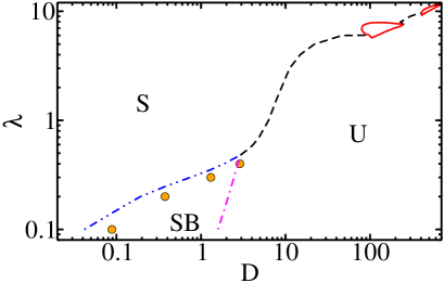
Figure 1: (Color online) Character of the energetically lowest lying stationary GP solution for $b=0.2a_{z}$ and $A=12E_{z}$: The dash-dot-dotted, dash-dotted and dashed lines indicate those $\lambda$ and $D$ values at which the character of the energetically lowest lying stationary GP solution with $k=0$ changes from symmetric (S) to symmetry-broken (SB), from symmetry-broken to unstable (U), and from symmetric to unstable, respectively. The “solid (red) islands” in the upper right corner of the phase diagram (comparatively large $D$ and $\lambda$) indicate two regions of the phase diagram where the solutions are symmetric but where the density maximum is located at $\rho>0$; these islands are discussed in more detail in the context of Fig. 5. For comparison, circles show the boundary between the symmetric and symmetry-broken regions predicted by the two mode model. Note the log scale of both axes.

The parameter combination $(\lambda,D)=(0.1,1)$ corresponds, e.g., to a Cr condensate with vanishing $s$-wave scattering length, $\omega_{z}=2\pi\times 10$Hz, $\omega_{\rho}=2\pi\times 100$Hz and $N\approx 1835$. The “phase diagram” consists of three regions: Firstly, a region where the energetically lowest lying state with $k=0$ of the stationary GP equation is symmetric with respect to the $z$-axis; we refer to this solution as symmetric (“S”) throughout this paper. Examplary density profiles are shown in Figs. 2(a), 2(c) and 2(d)

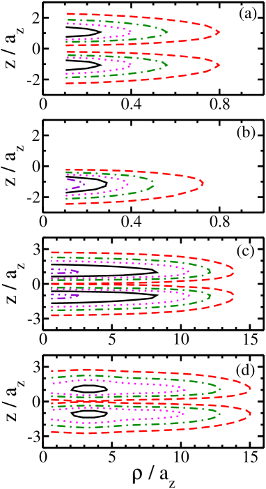
Figure 2: (Color online) Density plots of the energetically lowest lying stationary GP solution with $k=0$ for $b=0.2a_{z}$, $A=12E_{z}$ and four different $(D,\lambda)$ combinations: (a) $(D,\lambda)=(0.5477,0.3)$ (symmetric solution), (b) $(D,\lambda)=(1.643,0.3)$ (symmetry-broken solution), (c) $(D,\lambda)=(316.2,10)$ (symmetric solution with density maximum at $\rho=0$) and (d) $(D,\lambda)=(474.3,10)$ (symmetric solution with density maximum at $\rho>0$). The contour lines are chosen equidistant in all four panels. The dashed contours correspond to (a) $0.05a_{z}^{-3}$, (b) $0.1a_{z}^{-3}$, (c) $0.0001a_{z}^{-3}$ and (d) $0.0001a_{z}^{-3}$, while the solid contours correspond to (a) $0.35a_{z}^{-3}$, (b) $0.7a_{z}^{-3}$, (c) $0.0007a_{z}^{-3}$ and (d) $0.0007a_{z}^{-3}$.

(see below for more details). Secondly, a region where the energetically lowest lying state of the stationary GP equation is neither symmetric nor anti-symmetric with respect to the $z$-axis; we refer to this solution as symmetry-broken (“SB”) or asymmetric. An examplary density profile is shown in Fig. 2(b). And thirdly, a region where the stationary GP equation supports a high-density or collapsed solution but no gas-like solution. We refer to this solution as mechanically unstable (“U”). Sections IV.1 and IV.2 discuss the properties of the phase diagram in more detail for $\lambda\lesssim 1$ and $\lambda\gtrsim 1$, respectively.

IV.1 “Small” aspect ratio ($\lambda\lesssim 1$)

Figure 3(a) shows the energy contributions to the total energy per particle $E_{\mathrm{tot}}/N$ for $\lambda=0.3$ and $A=12E_{z}$ as a function of $D$:

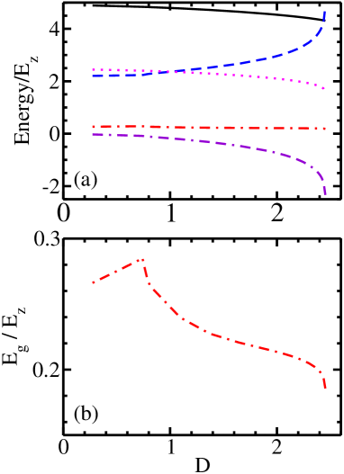
Figure 3: (Color online) (a) Energy contributions of the energetically lowest lying stationary GP solution with $k=0$ as a function of $D$ for $\lambda=0.3$, $A=12E_{z}$ and $b=0.2a_{z}$. The solid, dashed, dotted, dash-dotted and dash-dash-dotted lines show $E_{\mathrm{tot}}/N$, $E_{\mathrm{kin}}$, $E_{\mathrm{ho}}$, $E_{\mathrm{g}}$ and $E_{\mathrm{dip}}$, respectively. (b) Blow-up of the Gaussian energy $E_{\mathrm{g}}$. $E_{\mathrm{g}}$ exhibits a kink at $D\approx 0.75$, indicating the symmetry change (symmetric to symmetry-broken) of the energetically lowest lying stationary GP solution.

the kinetic energy per particle $E_{\mathrm{kin}}$ (dashed line); the harmonic trap energy per particle $E_{\mathrm{ho}}$ (dotted line), which is defined as the expectation value of $V_{\mathrm{ho}}$; the Gaussian energy per particle $E_{\mathrm{g}}$ (dash-dotted line), which is defined as the expectation value of $V_{\mathrm{g}}$; and the mean-field dipole-dipole energy per particle $E_{\mathrm{dip}}$ (dash-dash-dotted line), which is defined as the expectation value of the mean-field term [third term on the right hand side of Eq. (II.1)]. A solid line shows the total energy per particle $E_{\mathrm{tot}}/N$. The energies terminate at the critical value $D_{\mathrm{cr}}$ at which the stationary GP equation first supports a negative energy solution.

The Gaussian energy $E_{\mathrm{g}}$ is shown on an enlarged scale in Fig. 3(b). It can be seen that $E_{\mathrm{g}}$ shows a “kink” at $D\approx 0.75$. We find that the other energy contributions (i.e., $E_{\mathrm{kin}}$, $E_{\mathrm{ho}}$ and $E_{\mathrm{dip}}$) and $E_{\mathrm{tot}}/N$ exhibit kinks at the same $D$ value. These kinks are, however, less pronounced and not (or hardly) visible on the scale shown in Fig. 3(a). Our analysis shows that the $D$ values at which the kinks occur coincide with the $D$ values at which the density profiles of the energetically lowest lying stationary GP solutions change from symmetric to symmetry-broken. In most of our calculations for fixed $b$, $A$ and $\lambda$ but varying $D$, we use the kink in $E_{\mathrm{g}}$ to determine the $D$ value at which the character of the energetically lowest lying stationary GP solution changes and thus to obtain the dash-dot-dotted line in Fig. 1. The stability of the solutions around the symmetry to symmetry-broken transition is discussed in Sec. V in the context of Figs. 7 through 10.

The dash-dot-dotted lines in Fig. 1 can be reproduced qualitatively by the two-mode model (see circles in Fig. 1). To illustrate some aspects of the two-mode model, solid and dashed lines in Fig. 4 show $\Lambda$ [see Eq. (33)] as a function of $D$ for $\lambda=0.3$ and $0.4$, respectively, and $A=12E_{z}$ and $b=0.2a_{z}$. For $|\Lambda|\leq 1$ and positive $T$, the two-mode model predicts a symmetric stationary ground state. For $|\Lambda|>1$, a symmetry-broken solution is supported; if $T>0$ and $\Lambda<-1$, the symmetry-broken state has a lower energy than the symmetric state. Vertical arrows in Fig. 4 mark the $D$ values, $D\approx 1.31$ and $2.89$, at which the transition from symmetric to symmetry-broken occurs for $\lambda=0.3$ and $\lambda=0.4$, respectively. These two-mode model predictions (also shown as circles in Fig. 1) are slightly larger than the results obtained by solving the GP equation but predict the symmetric to

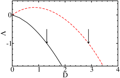
Figure 4: (Color online) Two-mode model parameter $\Lambda$ for $A=12E_{z}$ and $b=0.2a_{z}$ as a function of $D$ for $\lambda=0.3$ (solid line) and $\lambda=0.4$ (dashed line). Vertical arrows mark the $D$ values at which $|\Lambda|$ equals $1$; for $|\Lambda|<1$ and $>1$, the two-mode model predicts that the energetically lowest lying stationary state is symmetric and symmetry-broken, respectively.

symmetry-broken transition qualitatively correctly.

It is interesting to compare the behavior of $\Lambda$, which can be interpreted as the ratio between an effective interaction energy and twice the tunneling energy, for $\lambda=0.3$ and $0.4$ (solid and dashed lines in Fig. 4). For $\lambda=0.3$, an increase of the mean-field strength $D$ leads to a monotonic decrease of $\Lambda$. For $\lambda=0.4$, in contrast, $\Lambda$ first increases, reaches a maximum at $D\approx 0.87$ and then decreases monotonically. We find that the onsite energy $U$ and the offsite energy $B$ are both negative for all $D$ shown in Fig. 4. A change of the aspect ratio $\lambda$ effectively changes the strength of the dipole-dipole interaction, leading to a less attractive $U$ than $B$, and thus to a positive $\Lambda$, for small $D$ and $\lambda=0.4$. For $\lambda=0.3$, in contrast, the onsite energy $U$ is always more negative than the offsite energy $B$, resulting in a negative $\Lambda$ for all $D$.

In addition to the barrier height $A=12E_{z}$, we considered smaller barrier heights $A$, in particular $A=4E_{z}$ and $8E_{z}$, for a few selected $\lambda$ values. Our calculations suggest that the dash-dot-dotted line in Fig. 1 (i.e., the line that marks the symmetric to symmetry-broken transition) moves to larger $D$ values with decreasing $A$ while the dash-dotted line (i.e., the line that marks the symmetry-broken to unstable transition) remains approximately unchanged with decreasing $A$. The dependence of the dash-dot-dotted line on $A$ for fixed $\lambda$ and $b$ can be explained by applying the two-mode model. As $A$ decreases, the tunneling energy $T$ becomes more important compared to the absolute value of the effective interaction energy $U-B$. This implies that $|\Lambda|$ decreases with decreasing $A$ (for fixed $\lambda$ and $b$). Correspondingly, a larger $D$ is required for the two-mode model condition $|\Lambda|=1$, which signals the symmetric to symmetry-broken transition, to be fulfilled. The fact that the dash-dotted line in Fig. 1 remains to first order unchanged with decreasing $A$ is due to the fact that the density of the system prior to collapse is located predominantly in one of the wells. This implies that the density prior to collapse is only weakly dependent on $A$, thus explaining the comparatively small dependence of the dash-dotted line on $A$ for the parameter combinations investigated.

We note at this point that the linear stationary Schrödinger equation permits only symmetric and anti-symmetric solutions but no symmetry-broken solutions. This fact emphasizes that the transition from symmetric to symmetry-broken is driven by mean-field interactions. Furthermore, this fact implies that the symmetry-broken solution should disappear if sufficiently many higher order corrections to the mean-field GP equation are taken into account (see, e.g., Ref. ragh99 ). In this sense, the appearance of the symmetry-broken region in the phase diagram is an artefact of the mean-field formalism. It is, however, intimately related to the dynamical phenomena of Josephson oscillation and macroscopic quantum self-trapping, both of which have been observed experimentally for $s$-wave interacting BECs. We return to these considerations in Sec. V in the context of the discussion of Figs. 7 through 10.

IV.2 “Large” aspect ratio ($\lambda\gtrsim 1$)

Figure 5 shows an enlargement of the large $\lambda$ region of Fig. 1 using a linear scale for both $\lambda$ and $D$. The S₀ region of the phase diagram is characterized by GP solutions whose density maxima are located at $\rho=0$ [see Figs. 2(a) and 2(c) for examples] while the S_>0 region of the phase diagram is charactericed by GP solutions whose density maxima are located at $\rho>0$ [see Fig. 2(d) for an example].

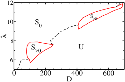
Figure 5: (Color online) Blow-up (with more detail) of the phase diagram for $b=0.2a_{z}$ and $A=12E_{z}$ shown in Fig. 1: The region where the energetically lowest lying symmetric stationary GP solution has its density maximum at $\rho=0$ is labeled by “S₀” and that where the energetically lowest lying symmetric stationary GP solution has its density maximum at $\rho>0$ by “S_>0”.

The latter class of density profiles only exists in a narrow parameter region of the phase diagram; in particular, these solutions only arise for pancake-shaped confining potentials and not for cigar-shaped confining potentials. Furthermore, the solutions with S_>0 character are unique to dipolar gases, i.e., they are not observed for purely $s$-wave interacting gases, and thus directly reflect the anisostropic long-range nature of the dipole-dipole interactions.

The two different classes of symmetric solutions have previously been characterized for $A=0$, i.e., for a pancake-shaped trapping geometry without barrier rone07 ; wils08 . In those studies, a dipolar BEC with density maximum at $\rho>0$ was termed “red blood cell”, as its isodensity surface is reminiscent of the shape of a red blood cell. The S_>0 regions in Fig. 5 are characterized by the formation of two staggered red blood cells. Section V shows that the dynamical instability near $D_{\mathrm{cr}}$ of the stationary $k=0$ ground state solutions of types S₀ and S_>0 is distinctly different.

Figure 5 shows that, generally speaking, the $D$ value at which the dipolar gas becomes unstable increases with increasing $\lambda$. This trend can be understood by realizing that an increase of $\lambda$ leads to a “flattening” of the system so that the dipoles interact effectively more repulsively. The boundary near the stable and unstable regions shows a rich structure: i) As already noted above, S_>0 islands in which the density profiles are structured exist. ii) The boundary between the S₀ and the U regions of the phase diagram changes non-monotonically. For $D\approx 240$, e.g., the system is mechanically stable for $\lambda\gtrsim 8.13$, mechanically unstable for $8.13\gtrsim\lambda\gtrsim 7.72$, and then again mechanically stable for a small $\lambda$ regime ($7.72\gtrsim\lambda\gtrsim 7.42$).

We find that some, though not all, of the features of the phase diagram can be reproduced qualitatively by a simple variational wave function $\psi_{var}(\rho,z)$,

$$\psi_{var}(\rho,z)=\left[\exp\left(-\frac{\rho^{2}}{2b_{1}^{2}}\right)+b_{2}\exp\left(-\frac{\rho^{2}}{2b_{3}^{2}}\right)\right]\times$$

$$\left[\exp\left(-\frac{z^{2}}{2b_{4}^{2}}\right)+b_{5}\left(1-\frac{z^{2}}{\lambda a_{z}^{2}}\right)\exp\left(-\frac{z^{2}}{2b_{6}^{2}}\right)\right],$$ (35)

where $b_{1}-b_{6}$ denote variational parameters that are optimized by minimizing the energy per particle. For $b_{2}=b_{5}=0$, $\psi_{var}$ reduces to the commonly used variational wave function of purely Gaussian shape. The second term in the first square bracket on the right hand side of Eq. (IV.2) has been added to allow for the description of densities of S_>0 character while the second term in the second square bracket on the right hand side of Eq. (IV.2) has been added to account for the Gaussian barrier along the $z$-direction. Figure 6 compares the total energy per particle from our variational calculation (dashed line) with that from the full numerical calculation (solid line) for $A=12E_{z}$, $\lambda=7$ and $b=0.2a_{z}$. The variational energy is less than 2 % higher than the energy obtained from the full numerical calculation. We find that the density of the dipolar gas changes from S₀ to S_>0 character at $D\approx 35$, compared to $D=80.03$ obtained from the full calculation.

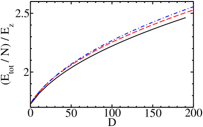
Figure 6: (Color online) A solid line shows the total energy per particle $E_{tot}/N$ of the energetically lowest lying stationary GP solution with $k=0$ as a function of $D$ for $\lambda=7$, $A=12E_{z}$ and $b=0.2a_{z}$ obtained numerically. For comparison, dashed and dash-dotted lines show $E_{tot}/N$ obtained using the variational six- and four-parameter variational wave functions (see text for details). The density of the system changes from S₀ to S_>0 character at $D\approx 35$ and $80.03$ for the six-parameter variational and the full numerical calculations, respectively.

For both sets of calculations, the energy and its derivative change smoothly as the system undergoes the structural change from S₀ to S_>0. For comparison, a dash-dotted line in Fig. 6 shows the energy per particle for $\psi_{var}$ with $b_{2}=0$ (we refer to this variational wave function as four-parameter wave function), i.e., for a wave function that is not sufficiently flexible to describe structured ground state densities of red blood cell shape. As expected, this variational wave function results in somewhat higher energies.

The variational wave function $\psi_{var}$ predicts S₀ to S_>0 transitions for all aspect ratios $\lambda$ between $5$ and $12$, indicating that it is not flexible enough to describe the island character of the S_>0 regions of the phase diagram and, furthermore, that the S₀ to S_>0 transition is driven by a delicate balance between the different energy contributions. Motivated by calculations presented in Ref. rone07 , we expect that the variational four-parameter wave function can qualitatively reproduce the existence of alternating stable and unstable regions of the phase diagram as $\lambda$ is changed for fixed $D$ and $A$ (see our discussion above for $D\approx 240$ and $A=12E_{z}$); we have, however, not checked this explicitly. Lastly, we note that the variational six-parameter wave function predicts a stable dipolar gas even for fairly large $D$ (i.e., $D$ values larger than those shown in Fig. 6) while the full numerical calculation predicts collapse at $D\approx 190.49$.

V Discussion of dynamical studies

This section presents Bogoliubov de Gennes excitation spectra and discusses the corresponding eigenmodes. For small $\lambda$ and appropriate $D$ (see Sec. V.1), the lowest non-vanishing Bogoliubov de Gennes excitation frequency is identified as the Josephson oscillation frequency $\omega_{\mathrm{J}}$. Comparisons with results obtained by time-evolving a properly prepared initial state and by applying the two-mode model equations are presented. In the regime where the symmetric solutions are of types $S_{0}$ and $S_{>0}$, respectively (large $\lambda$, see Sec. V.2), the decay mechanisms are identified. Furthermore, the character of various (avoided) crossings of the excitation frequencies is revealed.

V.1 “Small” aspect ratio ($\lambda\lesssim 1$)

Figure 7 shows the excitation spectrum as a function of $D$ obtained by solving the Bogoliubov de Gennes equations for $A=12E_{z}$, $b=0.2a_{z}$ and $\lambda=0.3$.

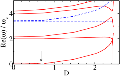
Figure 7: (Color online) Excitation spectrum obtained by solving the Bogoliubov de Gennes equations as a function of $D$ for $A=12E_{z}$, $b=0.2a_{z}$ and $\lambda=0.3$. The real parts of the frequencies for $k=0$ and 1 are shown by solid and dashed lines, respectively. The vertical arrow indicates the $D$ value, $D\approx 0.68$, at which the real part of the lowest non-vanishing $k=0$ Bogoliubov de Gennes frequency vanishes.

The spectrum is characterized by three distinct features that will be elaborated on in the following paragraphs: i) The real part of the lowest $k=0$ frequency vanishes at $D\approx 0.68$, and “reappears” at $D\approx 0.75$. ii) The $k=0$ frequencies show a series of crossings (or avoided crossings) at $D\approx 2.42$. iii) At slightly larger $D$ values, i.e., near $D\approx 2.45$, the real part of several $k=0$ excitation frequencies vanishes.

We first discuss the regime i) around $D\approx 0.68-0.75$. Figure 8(a) shows the

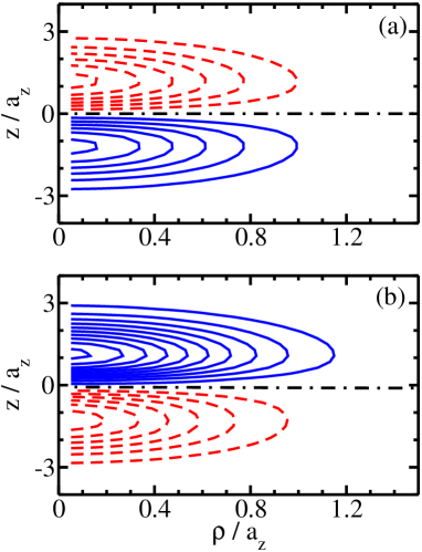
Figure 8: (Color online) Bogoliubov de Gennes eigenmodes $\bar{f}(\rho,z)$ corresponding to the lowest non-vanishing $k=0$ frequency for $\lambda=0.3$, $A=12E_{z}$, $b=0.2a_{z}$ and (a) $D=0.6573$ and (b) $D=0.7668$. The contours are chosen equidistant, with solid and dashed lines corresponding to positive and negative values of $\bar{f}$. The dash-dotted lines indicate the nodal lines of $\bar{f}$.

Bogoliubov de Gennes eigenmode $\bar{f}(\rho,z)$ that corresponds to the lowest non-vanishing $k=0$ frequency for $D=0.6573$, $A=12E_{z}$, $\lambda=0.3$ and $b=0.2a_{z}$. For these parameters, the energetically lowest lying stationary GP solution is symmetric and the corresponding eigenfrequency has a finite real part and vanishing imaginary part (see Fig. 7). Since Bogoliubov de Gennes functions with $k=0$ have no explicit $\varphi$ dependence, the eigenmode shown in Fig. 8(a) corresponds to a situation where the population oscillates with frequency $\omega$ between the left and the right well as a function of time. The lowest non-vanishing $k=0$ frequency can thus be identified as the Josephson oscillation frequency $\omega_{\mathrm{J}}$ (see also below). For comparison, Fig. 8(b) shows the Bogoliubov de Gennes eigenmode $\bar{f}(\rho,z)$ corresponding to the lowest non-vanishing $k=0$ frequency for $D=0.7668$ (i.e., in the regime where the frequency has “reappeared” and where the energetically lowest lying stationary GP solution with $k=0$ is symmetry-broken) and the same $A$, $E_{z}$ and $b$ values as before. In this case, the asymmetry of the eigenmode indicates that there is population transfer between the left and the right wells but that there is, on average, more population in the right than in the left well. This behavior is identified as macroscopic quantum self-trapping. Our interpretation of the Bogoliubov de Genne eigenmodes is supported by our time-dependent calculations.

In our time-dependent studies near the symmetric to symmetry-broken transition, we prepare an initial state and time evolve it according to the mean-field Hamiltonian $H$, Eq. (II.1). As for $s$-wave interacting BECs, the system dynamics can be divided into two categories (see also above): A regime where the population is transferred back and forth between the left well and the right well (this is the Josephson oscillation regime) and a regime where the time averaged population is asymmetrically divided among the two wells (this is the macroscopic quantum self-trapping regime). Figures 9(a) and 9(b) show the time evolution of

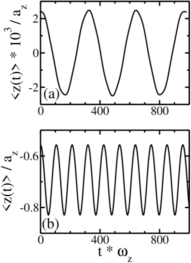
Figure 9: (Color online) Solid lines show the expectation value $\langle z(t)\rangle$ (see text)—calculated by time evolving a given initial state according to the mean-field Hamiltonian, Eq. (II.1)—as a function of time $t$ for $A=12E_{z}$, $\lambda=0.3$, $b=0.2a_{z}$ and (a) $D=0.6573$ (Josephson oscillation regime) and (b) $D=0.7668$ (macroscopic quantum self-trapping regime). In panel (a), the initial state is prepared according to Eq. (22) with $Z(0)=0.002$ and $\phi(0)=0$. In panel (b), the initial state is prepared by adding a small amount of random noise to the energetically lowest lying stationary GP solution.

the expectation value $\langle z(t)\rangle$ for $D=0.6573$ and $D=0.7668$, respectively. Here, $\langle z(t)\rangle$ is obtained by calculating the expectation value of $z$ with respect to the GP density at each time step. The expectation value $\langle z(t)\rangle$ is related to but not identical to the population difference $Z(t)$ introduced in Sec. III. For these $D$ values, the energetically lowest lying stationary GP solution is symmetric and symmetry-broken, respectively. For $D=0.6573$, the initial state is prepared according to Eq. (22) with $\phi(0)=0$ and $Z(0)=0.002$. Figure 9(a) shows that $\langle z(t)\rangle$ oscillates between positive and negative values of equal magnitude and that the time average of $\langle z(t)\rangle$ over a period gives zero. For $D=0.7668$, the initial state is prepared by adding a small amount of random noise to the energetically lowest lying stationary GP solution. Figure 9(b) shows that $\langle z(t)\rangle$ oscillates about a negative value and that the time average of $\langle z(t)\rangle$ gives a non-zero value. An analysis of the time evolution of the density profiles confirms that the system is in the Josephson regime and in the macroscopic quantum self-trapping regime, respectively.

To determine the oscillation frequency from the time evolution of $\langle z(t)\rangle$, we Fourier transform $\langle z(t)\rangle$ and record the center of the dominant peak for various parameter combinations. Circles in Fig. 10

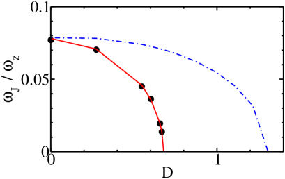
Figure 10: (Color online) Josephson oscillation frquency $\omega_{\mathrm{J}}$ as a function of $D$ for $\lambda=0.3$, $A=12E_{z}$ and $b=0.2a_{z}$. The circles show the Josephson oscillation frequency $\omega_{\mathrm{J}}$ obtained from our time-dependent study, in which the initial state is prepared according to Eq. (22) with $Z(0)=0.002$ and $\phi(0)=0$ and then time evolved according to the mean-field Hamiltonian $H$, Eq. (II.1). The solid line shows the lowest non-vanishing $k=0$ Bogoliubov de Gennes excitation frequency. For comparison, a dash-dotted line shows the two-mode model prediction $\omega_{\mathrm{J,TM}}$.

show the resulting Josephson oscillation frequency $\omega_{\mathrm{J}}$ for $A=12E_{z}$, $\lambda=0.3$ and $b=0.2a_{z}$. The agreement between the frequency obtained from the Fourier analysis (circles in Fig. 10) and the lowest non-vanishing $k=0$ Bogoliubov de Gennes excitation frequency (solid line in Fig. 10) is excellent. The $D$ value at which the Josephson oscillation frequency obtained by Fourier transforming $\langle z(t)\rangle$ vanishes, coincides, within our numerical accuracy, with that at which the lowest non-vanishing $k=0$ Bogoliubov de Gennes excitation frequency becomes imaginary. Notably, this $D$ value, $D\approx 0.68$, is slightly smaller than the $D$ value at which the energetically lowest lying stationary GP solution changes from symmetric to symmetry-broken ($D\approx 0.75$).

We find that the lowest non-vanishing $k=0$ Bogoliubov de Gennes frequency for $D=0.7668$ and $\lambda=0.3$ is about 30% smaller than the oscillation frequency extracted from Fig. 9(b), i.e., $\omega=0.059\omega_{z}$. The fact that the Bogoliubov de Gennes excitation frequency differs notably from the frequency obtained by Fourier-transforming $\langle z(t)\rangle$ might be due to the approximate nature of the Bogoliubov de Gennes equations.

For comparison, a dash-dotted line in Fig. 10 shows the Josephson oscillation frequency $\omega_{\mathrm{J,TM}}$, Eq. (34), predicted by the two-mode model. Figure 10 shows that the two-mode model provides a qualitatively but not quantitatively correct description of the Josephson oscillation frequency. The fact that the two-mode model does not allow for quantitative predictions for all $D$ is likely due to the fact that the modes $\Phi_{\mathrm{L}}$ and $\Phi_{\mathrm{R}}$ are not entirely located in the left well and in the right well, respectively, but that the left mode “leaks” into the right well and the right mode into the left well. This has been discussed in some detail in Ref. xion09 , which employs a slightly modified version of the two-mode model. In an attempt to obtain a better simple quantitative description of the system dynamics, we applied the improved two-mode model proposed in Ref. anan06 . For the cases considered, we find that this model leads only to small changes compared to the simple two-mode model applied above and does not provide a significantly improved description. In the future, it may be interesting to apply a multi-mode model.

We now discuss the regime ii) near $D\approx 2.42$, where the $k=0$ frequencies show (avoided) crossings. To shed light on these (avoided) crossings, Figs. 11(a)-(d) show the Bogoliubov de Gennes eigenmodes $\bar{f}(\rho,z)$ corresponding to the four lowest non-vanishing $k=0$ frequencies just before the crossing (i.e., for $D=2.410$), while Figs. 11(e)-(h) show those corresponding to the four lowest $k=0$ frequencies just after the crossing (i.e., for $D=2.443$).

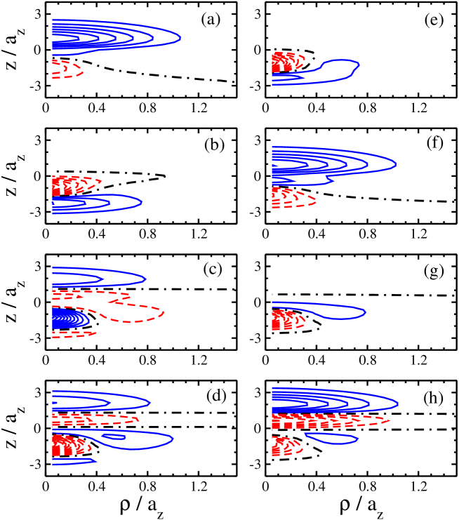
Figure 11: (Color online) Bogoliubov de Gennes eigenmodes $\bar{f}(\rho,z)$ corresponding to the four lowest non-vanishing $k=0$ frequencies for $\lambda=0.3$, $A=12E_{z}$, $b=0.2a_{z}$. Panels (a)-(d) show $\bar{f}$ corresponding to the lowest, second lowest, third lowest and fourth lowest frequencies for $D=2.410$ (i.e., just before the crossing) while panels (e)-(h) show $\bar{f}$ corresponding to the lowest, second lowest, third lowest and fourth lowest frequencies for $D=2.443$ (i.e., just after the crossing). The contours are chosen equidistant, with solid and dashed lines corresponding respectively to positive and negative values of $\bar{f}$.

Dash-dotted lines in Fig. 11 indicate the nodal lines of the Bogoliubov de Gennes eigenmodes. While some of these nodal lines are to first order only dependent on $z$, others depend in a non-trivial manner on $\rho$ and $z$. In the following we discuss a few key features of the eigenmodes shown in Fig. 11. The eigenmode corresponding to the lowest frequency extends over both wells just before the crossing [see Fig. 11(a)] and is located predominantly in one of the wells just after the crossing [see Fig. 11(e)]. The eigenmode corresponding to the second lowest non-vanishing frequency, in turn, is located predominantly in one of the wells just before the crossing [see Fig. 11(b)] and extends over both wells just after the crossing [see Fig. 11(f)]. The third and fourth lowest excitation frequencies show an avoided crossing at $D\approx 2.41$ (see Fig. 7). The eigenmode corresponding to the third lowest non-vanishing $k=0$ frequency has a fairly small amplitude in the right well before the avoided crossing [see Fig. 11(c)]; after the avoided crossing, the eigenmode corresponding to the third lowest $k=0$ frequency is located essentially entirely in the left well [see Fig. 11(g)]. The eigenmode corresponding to the forth lowest frequency, in turn, changes comparatively little as $D$ increases [see Figs. 11(d) and 11(h)].

Next, we turn to regime iii) near $D\approx 2.45$, where the real part of several $k=0$ Bogoliubov de Gennes excitation frequencies vanishes. The softening of these frequencies is inherently related to the transition from the stable symmetry-broken region to the unstable region of the phase diagram. The Bogoliubov excitation spectrum for $A_{z}=12E_{z}$, $\lambda=0.3$ and $b=0.2a_{z}$ shows that the real part of the lowest $k=0$ frequency vanishes at $D\approx 2.45$, which is slightly smaller than the $D$ value at which the stationary GP equation starts supporting unbounded negative energy solutions. In particular, for the parameter combination considered, the difference is about 0.6%. The Bogoliubov de Gennes excitation spectrum indicates that the collapse is triggered by the lowest $k=0$ mode. The corresponding eigenmode [see Fig. 11(e)] shows that, as might be expected naively, the density grows appreciably in the well that supports the majority of the population. This interpretation is supported by our time-dependent studies. Following the lowest $k=0$ mode, the eigenmode corresponding to the third lowest non-vanishing $k=0$ frequency becomes soft. As indicated in Fig. 11(g), this eigenmode is, not unexpectedly, also located predominately in one of the wells. To summarize, the collapse of the system can be characterized as a global collapse in which the density maximum increases in one of the wells, with the density maximum being located at $\rho=0$.

V.2 “Large” aspect ratio ($\lambda\gtrsim 1$)

This section discusses selected Bogoliubov de Gennes excitation spectra for larger $\lambda$. In particular, we focus on $\lambda=5$ and $\lambda=7$, for which the energetically lowest lying stationary GP solution prior to collapse is of type $S_{0}$ and $S_{>0}$, respectively.

Figure 12 shows the excitation spectrum as a function of $D$ for $\lambda=5$, $A=12E_{z}$ and $b=0.2a_{z}$.

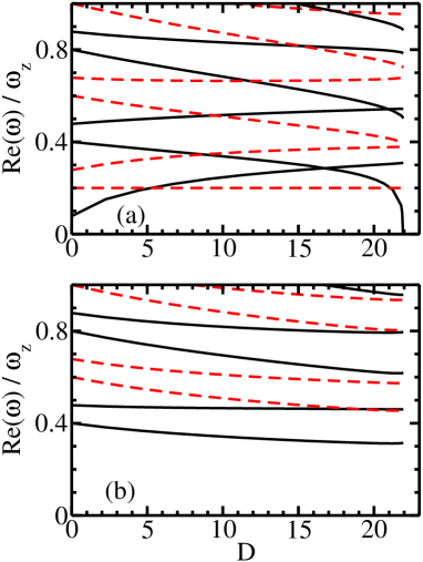
Figure 12: (Color online) Excitation spectrum obtained by solving the Bogoliubov de Gennes equations as a function of $D$ for $A=12E_{z}$, $b=0.2a_{z}$ and $\lambda=5$. Solid and dashed lines in panel (a) show the real parts of the Bogoliubov de Gennes excitation frequencies for $k=0$ and $1$, while solid and dashed lines in panel (b) show those for $k=2$ and $3$.

The two lowest non-vanishing $k=0$ frequencies [solid lines in Fig. 12(a)] cross at $D\approx 17$. Prior to the crossing, the lowest $k=0$ frequency corresponds to an eigenmode whose nodal line is parameterized by $z=0$ [see dash-dotted line in Fig. 13(a)]. Correspondingly, the eigen mode describes density oscillations between the left and the right well with, on average, equal densities in each of the two wells. For $D\approx 17-22$ (i.e., after the crossing), the nodal line of the lowest non-vanishing $k=0$ eigenmode is to a good approximation independent of $z$ and can be parametrized by $\rho\approx 2a_{z}$ to $\approx 3a_{z}$. As an example, Fig. 13(b) shows the

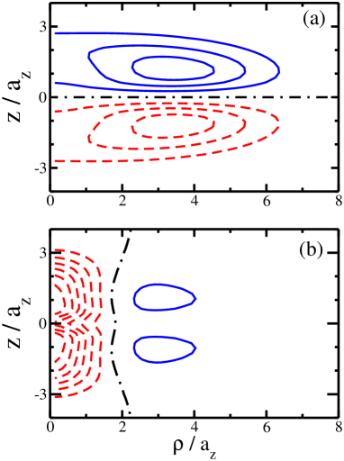
Figure 13: (Color online) Bogoliubov de Gennes eigenmodes $\bar{f}(\rho,z)$ corresponding to the lowest non-vanishing $k=0$ frequency for $\lambda=5$, $A=12E_{z}$, $b=0.2a_{z}$ and (a) $D=13.42$ and (b) $D=21.87$. The contours are chosen equidistant, with solid and dashed lines corresponding to positive and negative values of $\bar{f}$. The dash-dotted lines indicate the nodal line of $\bar{f}$.

eigenmode for $D=21.87$, which is just slightly smaller than the $D$ value at which the real part of the corresponding Bogoliubov de Gennes frequency vanishes. In particular, the lowest Bogoliubov de Gennes mode becomes soft at $D\approx 21.92$ while the stationary GP equation ceases to a support a positive energy solution with $k=0$ at a somewhat larger $D$ value, namely at $D\approx 22.03$.

Figures 12 and 13(b) suggest that the collapse of the system is triggered by the lowest $k=0$ mode and that the collapse is associated with an increase of the peak density at $\rho=0$ in each of the two wells. The collapse can thus be characterized as a local collapse as opposed to a global collapse. The local nature of the collapse (i.e., the fact that the peak density grows simultaneously in two distinct regions) can be traced back directly to the presence of the comparatively large Gaussian barrier. The chemical potential $\mu$ takes values around $2E_{z}$ for the parameter range considered in Fig. 12 and is thus significantly smaller than the barrier height $A$, $A=12E_{z}$. In the limit that the Gaussian barrier vanishes rone07 , the collapse becomes global. In this case, a similar nodal pattern of the eigenmode was found (see Fig. 2Ic of Ref. rone07 ; the larger number of nodal lines in this plot can be traced back to the larger $\lambda$ value) and the collapse is associated with a radial roton.

Figure 14 shows the Bogoliubov de Gennes excitation spectrum for $\lambda=7$, $A=12E_{z}$ and $b=0.2a_{z}$. For this parameter combination, the energetically lowest lying stationary GP solution deviates from the “structureless Gaussian shape” prior to collapse and is instead characterized by a density whose maximum is located at $\rho>0$, i.e., the density is of type S_>0 prior to collapse (see Fig. 2 for a density profile of type S_>0 for a somewhat larger $\lambda$).

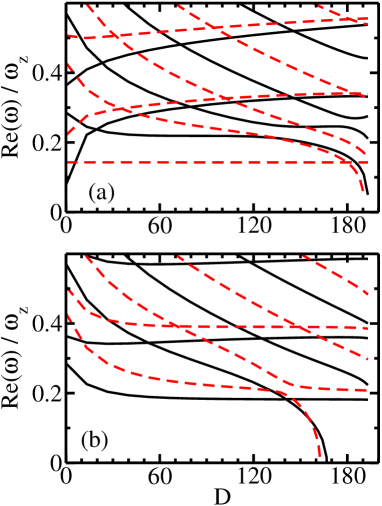
Figure 14: (Color online) Excitation spectrum obtained by solving the Bogoliubov de Gennes equations as a function of $D$ for $A=12E_{z}$, $b=0.2a_{z}$ and $\lambda=7$. Solid and dashed lines in panel (a) show the real parts of the Bogoliubov de Gennes excitation frequencies for $k=0$ and $1$, while solid and dashed lines in panel (b) show those for $k=2$ and $3$.

The Bogoliubov de Gennes excitation spectrum shown in Figs. 14(a) and 14(b) is rich, with a series of crossings and avoided crossings. Here, we focus on the large $D$ regime. Figures 14(a) and 14(b) show that the lowest $k=3$ mode becomes soft first, followed by the lowest $k=2$, $k=1$ and $k=0$ modes. This indicates that the collapse is triggered by a mode with non-vanishing azimuthal quantum number, similarly to the case with vanishing barrier height rone07 . The $D$ value, $D\approx 163$, at which the $k=3$ mode becomes soft is about 16% smaller than the $D$ value at which the stationary GP equation first supports negative energy solutions. This implies an appreciable reduction of the S_>0 islands shown in Figs. 1 and 5.

It is worth emphasizing at this point that the fact that the $k=3$ mode becomes soft first is not specific to the double-well geometry considered here; in fact, decay triggered by the $k=3$ mode has also been found for pancake-shaped dipolar gases without barrier (see Ref. rone07 and below). While Fig. 14 shows an example where the $k=3$ mode becomes soft first, we find that the collapse can—again, just as in the case of vanishing barrier rone07 —also be triggered by other finite $k$ modes. For example, for a somewhat smaller barrier height but the same barrier width and aspect ratio as in Fig. 14 (i.e., for $A=9E_{z}$, $b=0.2a_{z}$ and $\lambda=7$), we find that the $k=2$ mode becomes soft first, followed by the $k=3$ and $k=1$ modes (our calculations included modes $k=0$ through $4$). In the following, we analyze the collapse triggered by the $k=3$ mode in more detail.

Figure 15 shows the eigenmodes associated with the two lowest $k=3$ Bogoliubov de Gennes frequencies for $D=119.1$ [Figs. 15(a) and 15(b)] and $D=161.4$ [Figs. 15(c) and 15(d)].

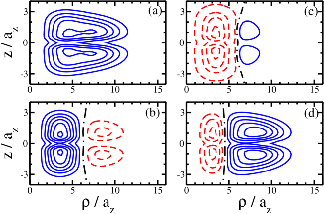
Figure 15: (Color online) Bogoliubov de Gennes eigenmodes $\bar{f}(\rho,z)$ corresponding to the two lowest non-vanishing $k=3$ frequencies for $\lambda=7$, $A=12E_{z}$ and $b=0.2a_{z}$. Panels (a) and (b) show the eigenmodes corresponding to the lowest and second lowest non-vanishing $k=3$ Bogoliubov de Gennes frequencies for $D=119.1$ (i.e., prior to the avoided crossing at $D\approx 140$), while panels (c) and (d) show those for $D=161.4$ (i.e., just prior to the lowest $k=3$ mode becoming soft). The contours are chosen equidistant, with solid and dashed lines corresponding to positive and negative values of $\bar{f}$. The dash-dotted lines indicate the nodal lines of $\bar{f}$.

Figure 15 shows that the eigenmode corresponding to the lowest non-vanishing $k=3$ frequency has no nodal line prior to the avoided crossing at $D\approx 140$ [see Fig. 15(a)] but one nodal line, which can be parametrized roughly by $\rho\approx 6a_{z}$ (or, equivalently by $\rho\approx 2.6a_{\rho}$), just prior to collapse [see Fig. 15(c)]. Importantly, the eigenmode remains symmetric with respect to $z=0$ even close to collapse and exhibits two equivalent extrema at positive and negative $z$. This suggests that the collapse is associated with a total of six density peaks, three located on a ring of the red blood cell located in the left well and three located on a ring of the red blood cell located in the right well. The collapse can thus be characterized as local, with the local character arising from i) the angular roton like nature of the instability and ii) the presence of the Gaussian barrier.

It is interesting to compare the eigenmodes for systems with vanishing and finite barrier in the regime where the first Bogoliubov de Gennes mode becomes soft. To this end, Fig. 16 shows the eigenmodes

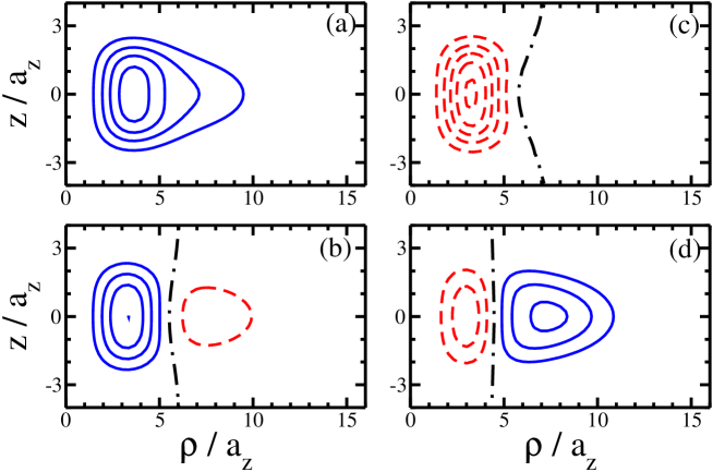
Figure 16: (Color online) Bogoliubov de Gennes eigenmodes $\bar{f}(\rho,z)$ corresponding to the two lowest non-vanishing $k=3$ frequencies for $\lambda=7$, $A=0$ and $b=0.2a_{z}$. Panels (a) and (b) show the eigenmodes corresponding to the lowest and second lowest non-vanishing $k=3$ Bogoliubov de Gennes frequencies for $D=66.14$, while panels (c) and (d) show those for $D=81.49$ (i.e., just prior to the lowest $k=3$ mode becoming soft). The contours are chosen equidistant, with solid and dashed lines corresponding to positive and negative values of $\bar{f}$. The dash-dotted lines indicate the nodal lines of $\bar{f}$.

corresponding to the two lowest non-vanishing $k=3$ frequencies for two different $D$ values, i.e., for $D=66.14$ and $D=81.49$, and $\lambda=7$ and $A=0$. The latter $D$ value corresponds to that investigated in Fig. 2II of Ref. rone07 . While we find that our excitation spectrum for $A=0$ (not shown here) agrees with Fig. 2IIb of Ref. rone07 , our eigenmode corresponding to the lowest non-vanishing $k=3$ frequency differs. In fact, we find that the eigenmode shown in Fig. 2IIc for $D=81.49$ converttorho corresponds to the second lowest and not to the lowest non-vanishing $k=3$ Bogoliubov de Gennes eigen frequency as stated in Ref. rone07  agreementwithronen . The eigenmode shown in Fig. 16(c) for $A=0$ and $D=81.49$ has a nodal line very similar to that shown in Fig. 15(c) for $A=12E_{z}$ and $D=161.4$, i.e., for a $D$ value that is roughly twice as large as that for $A=0$. The main difference between the two eigenmodes is that the latter is characterized by extrema at $z\approx\pm a_{z}$ as opposed to $z=0$.

VI Summary and Outlook

This paper presents a detailed mean-field analysis of a purely dipolar BEC in a cylindrically symmetric external confining potential with repulsive Gaussian barrier centered at $z=0$. The dipoles are assumed to be aligned along one of the symmetry axes of the confining potential, which can be realized experimentally through the application of an external field. We have investigated the behaviors of the system as functions of the dimensionless parameter $D$, which is defined as the product of the number of particles and the square of the magnitude of the dipole moment $d$, the aspect ratio $\lambda$ and, in a few selected cases, the height $A$ of the Gaussian barrier. Throughout, the barrier width $b$ and the $s$-wave scattering length $a_{s}$ were kept fixed at $b=0.2a_{z}$ and $a_{s}=0$, respectively. The energetics and the density profiles obtained by solving the stationary GP equation have been discussed and the onset of the mechanical instability has been analyzed. Additional insights were gained from a dynamical stability analysis, which is based on time-evolving a given initial state or on the Bogoliubov de Gennes excitation spectrum. The latter was complemented by a detailed analysis of selected Bogoliubov de Gennes eigenmodes.

For sufficiently small aspect ratios, i.e., for cigar-shaped harmonic traps in which the dipoles are aligned along the weak confinement direction, the energetically lowest lying stationary ground state solution is either symmetric or symmetry-broken. As in the case of $s$-wave interacting BECs, the appearance of these solutions can be explained qualitatively within a two-mode model. For a critical mean-field strength $D_{\mathrm{cr}}$, the system becomes unstable. The Bogoliubov de Gennes framework reveals that the collapse occurs globally, i.e., within a single well, with the decay being triggered by a mode with vanishing azimuthal quantum number.

As the aspect ratio $\lambda$ increases, the region of the phase diagram where the energetically lowest lying stationary GP solution is symmetry-broken vanishes. For sufficiently large aspect ratio $\lambda$, the symmetric solutions fall into one of two classes: The system’s density is characterized by a density maximum at $\rho=0$ (this is referred to as S₀ type) or by a density maximum at $\rho>0$ (this is referred to as S_>0 type). The latter class of solutions occupies a fairly small region of the phase diagram and only occurs near the dynamical instability line and only for certain aspect ratios $\lambda$ and barrier heights $A$. For a barrier height of $A=12E_{z}$ and $\lambda=7$, e.g., the solution is of type S_>0 prior to collapse. Correspondingly, we find that the collapse occurs locally through a mode with finite azimuthal quantum number ($k=3$), with density spikes emerging in six different regions of the trap. Three of these density peaks grow in the left well and three in the right well. Furthermore, each of the three density peaks lies on a ring that is associated with the density maximum of the ground state solution at $\rho>0$. The instability can, as in the case of a vanishing Gaussian barrier, be characterized as an angular roton instability. We note, however, that the radial degrees of freedom also play a role, i.e., that the Bogoliubov de Gennes eigenmodes prior to collapse contain radial nodal lines. For pancake-shaped trapping geometries (i.e., for $\lambda>1$), this paper primarily explored the $(D,\lambda)$ parameter space for fixed $A$. We find that the double well system exhibits a number of novel and rich stability characteristics as the barrier height $A$ is varied; these studies will be reported on in a forthcoming article asad09 .

Our theoretical predictions for purely dipolar BECs presented in this paper can be tested experimentally by loading a dipolar BEC such as a Cr BEC into a double well potential and by tuning the $s$-wave scattering length to zero through the application of an external magnetic field in the vicinity of a magnetic Feshbach resonance. Following the spirit of the double-well experiments for $s$-wave interacting BECs (see, e.g., Ref. albi05 ), it should be possible to study the transition from the Josephson tunneling regime to the macroscopic quantum self-trapping regime by loading the double well system with varying number of particles and varying population difference in the left and right wells. For pancake-shaped harmonic confinement, we suggest an experimental sequence that would allow the stability lines discussed in the context of Fig. 5 to be probed. We suggest to increase the radial trapping frequency $\omega_{\rho}$ (and to thus decrease $\lambda$) for fixed $A$ and to monitor the loss of atoms from the trap. This scenario corresponds to approaching the instability line in Fig. 5 vertically from above. By repeating this experiment for condensates with varying number of particles, the different collapse mechanisms associated with the S₀ regions and the S_>0 islands could be probed (see also Ref. wilsonmostrecent ).

In the future, it will be interesting to investigate how the behaviors of the system change as a function of the “spacing” between the left and the right well, i.e., as a function of the barrier widths $b$. The present study covers the regime where the “spacing” between the left and the right well is comparatively small, i.e., where it is comparable to the axial confinement length, and where the system is described by one macroscopic wave function. Our approach for pancake-shaped confinement with Gaussian barrier is distinctly different from other recent studies of multi-layer (quasi-)two-dimensional dipolar BECs wang08 ; kobe09 , which assume that the dipoles in neighboring wells feel each other but that the distance between the neighboring wells is so large that each dipole can be assigned to a specific well. In this case, the system has been discretized, leading to a coupled set of equations that have been solved self-consistently. It will be interesting to extend the present study of pancake-shaped two-well systems to a regime where comparisons with a discretized description become meaningful. It will also be interesting to extend the present work to multi-well traps. In the regime of small aspect ratio, e.g., a three- or four-well system might lead to interesting dynamics that can be controlled by varying the onsite and the offsite interactions. In this case, a multi-mode analysis suggests itself as a first starting point.

Support by the NSF through grants PHY-0555316 and PHY-0855332 is gratefully acknowledged.

References

- (1) M. A. Baranov, Physics Reports 464, 71 (2008).
- (2) T. Lahaye, C. Menotti, L. Santos, M. Lewenstein, and T. Pfau, arXiv:0905.0386 (2009).
- (3) A. Griesmaier, J. Werner, S. Hensler, J. Stuhler, and T. Pfau, Phys. Rev. Lett. 94, 160401 (2005).
- (4) J. Stuhler, A. Griesmaier, T. Koch, M. Fattori, T. Pfau, S. Giovanazzi, P. Pedri, and L. Santos, Phys. Rev. Lett. 95, 150406 (2005).
- (5) J. Werner, A. Griesmaier, S. Hensler, J. Stuhler, T. Pfau, A. Simoni and E. Tiesinga, Phys. Rev. Lett. 94, 183201 (2005).
- (6) T. Koch, T. Lahaye, J. Metz, B. Fröhlich, A. Griesmaier, and T. Pfau, Nature Physics 4, 218 (2008).
- (7) T. Lahaye, J. Metz, B. Fröhlich, T. Koch, M. Meister, A. Griesmaier, T. Pfau, H. Saito, Y. Kawaguchi, and M. Ueda, Phys. Rev. Lett. 101, 080401 (2008).
- (8) L. Santos, G. V. Shlyapnikov, P. Zoller, and M. Lewenstein, Phys. Rev. Lett. 85, 1791 (2000).
- (9) S. Yi and L. You, Phys. Rev. A 61, 041604(R) (2000).
- (10) S. Yi and L. You, Phys. Rev. A 63, 053607 (2001).
- (11) K. Goral and L. Santos, Phys. Rev. A 66, 023613 (2002).
- (12) C. Eberlein, S. Giovanazzi, and D. H. J. O’Dell, Phys. Rev. A 71, 033618 (2005).
- (13) D. C. E. Bortolotti, S. Ronen, J. L. Bohn, and D. Blume, Phys. Rev. Lett. 97, 160402 (2006).
- (14) U. R. Fischer, Phys. Rev. A 73, 031602(R) (2006).
- (15) S. Ronen, D. C. E. Bortolotti, and J. L. Bohn, Phys. Rev. Lett. 98, 030406 (2007).
- (16) O. Dutta and P. Meystre, Phys. Rev. A 75, 053604 (2007).
- (17) J. Metz, T. Lahaye, B. Fröhlich, A. Griesmaier, T. Pfau, H. Saito, Y. Kawaguchi, and M. Ueda, New J. Phys. 11, 055032 (2009).
- (18) S. Giovanazzi, D. O’Dell, and G. Kurizki, Phys. Rev. Lett. 88, 130402 (2002).
- (19) L. Santos, G. V. Shlyapnikov, and M. Lewenstein, Phys. Rev. Lett. 90, 250403 (2003).
- (20) N. R. Cooper, E. H. Rezayi, and S. H. Simon, Phys. Rev. Lett. 95, 200402 (2005).
- (21) J. Zhang and H. Zhai, Phys. Rev. Lett. 95, 200403 (2004).
- (22) S. Yi and H. Pu, Phys. Rev. A 73, 061602(R) (2006).
- (23) D. H. J. O’Dell and C. Eberlein, Phys. Rev. A 75, 013604 (2007).
- (24) R. M. Wilson, S. Ronen, and J. L. Bohn, Phys. Rev. A 79, 013621 (2009).
- (25) K. Góral, L. Santos, and M. Lewenstein, Phys. Rev. Lett. 88, 170406 (2002).
- (26) B. Damski, L. Santos, E. Tiemann, M. Lewenstein, S. Kotochigova, P. Julienne, and P. Zoller, Phys. Rev. Lett. 90, 110401 (2003).
- (27) C. Menotti, C. Trefzger, and M. Lewenstein, Phys. Rev. Lett. 98, 235301 (2007).
- (28) L. E. Sadler, J. M. Higbie, S. R. Leslie, M. Vengalatorre, and D. M. Stamper-Kurn, Nature 443, 312 (2006).
- (29) M. Vengalatorre, S. R. Leslie, J. Guzman, and D. M. Stamper-Kurn, Phys. Rev. Lett. 100, 170403 (2008).
- (30) M. Fattori, G. Roati, B. Deissler, C. D’Errico, M. Zaccanti, M. Jona-Lasinio, L. Santos, M. Inguscio, and G. Modugno, Phys. Rev. Lett. 101, 190405 (2008).
- (31) S. E. Pollack, D. Dries, M. Junker, Y. P. Chen, T. A. Corcovilos, and R. G. Hulet, Phys. Rev. Lett. 102, 090402 (2009).
- (32) K.-K. Ni, S. Ospelkaus, M. H. G. de Miranda, A. Pe’er, B. Neyenhuis, J. J. Zirbel, S. Kotochigova, P. S. Julienne, D. S. Jin, and J. Ye, Science 322, 231 (2008).
- (33) J. Deiglmayr, A. Grochola, M. Repp, K. Mortlbauer, C. Gluck, J. Lange, O. Dulieu, R. Wester, and M. Weidemüller, Phys. Rev. Lett. 101, 133004 (2008).
- (34) J. G. Danzl, E. Haller, M. Gustavsson, M. J. Mark, R. Hart, N. Bouloufa, O. Dulieu, H. Ritsch, and H.-C. Nägerl, Science 321, 1062 (2008).
- (35) M. Marinescu and L. You, Phys. Rev. Lett. 81, 4596 (1998).
- (36) M. Lewenstein, A. Sanpera, V. Ahufinger, B. Damski, A. Sen De, and U. Den, Adv. Phys. 56, 243 (2007).
- (37) I. Bloch, J. Dalibard, and W. Zwerger, Rev. Mod. Phys. 80, 885 (2008).
- (38) S. Aubry, S. Flach, K. Kladko, and E. Olbrich, Phys. Rev. Lett. 76, 1607 (1996).
- (39) A. Smerzi, S. Fantoni, S. Giovanazzi, and S. R. Shenoy, Phys. Rev. Lett. 79, 4950 (1997).
- (40) B. P. Anderson and M. A. Kasevich, Science 282, 1686 (1998).
- (41) S. Raghavan, A. Smerzi, S. Fantoni, and S. R. Shenoy, Phys. Rev. A 59, 620 (1999).
- (42) S. Giovanazzi, A. Smerzi, and S. Fantoni, Phys. Rev. Lett. 84, 4521 (2000).
- (43) F. S. Cataliotti, S. Burger, C. Fort, P. Maddaloni, F. Minardi, A. Trombettoni, A. Smerzi, and M. Inguscio, Science 293, 843 (2001).
- (44) M. Albiez, R. Gati, J. Folling, S. Hunsmann, M. Cristiani, and M. K. Oberthaler, Phys. Rev. Lett. 95, 010402 (2005).
- (45) D. Ananikian and T. Bergeman, Phys. Rev. A 73, 013604 (2006).
- (46) R. Gati and M. K. Oberthaler, J. Phys. B 40, 61R (2007).
- (47) J. Esteve, C. Gross, A. Weller, S. Giovanazzi, and M. K. Oberthaler, Nature 455, 1216 (2008).
- (48) Y. Shin, M. Saba, T. A. Pasquini, W. Ketterle, D. E. Pritchard, and A. E. Leanhardt, Phys. Rev. Lett. 92, 050405 (2004).
- (49) B. Xiong, J. B. Gong, H. Pu, W. Z. Bao, and B. W. Li, Phys. Rev. A 79, 013626 (2009).
- (50) D.-W. Wang and E. Demler, arXiv:0812.1838 .
- (51) M. Klawunn and L. Santos, Phys. Rev. A 80, 013611 (2009).
- (52) P. Köberle and G. Wunner, arXiv:0908.1009 (2009).
- (53) K. Goral, K. Rzazewski, and T. Pfau, Phys. Rev. A 61, 051601(R) (2000).
- (54) S. Ronen, D. C. E. Bortolotti, and J. L. Bohn, Phys. Rev. A 74, 013623 (2006).
- (55) M. Modugno, L. Pricoupenko, and Y. Castin, Eur. Phys. J. D 22, 235 (2003).
- (56) F. Dalfovo, S. Giorgini, L. P. Pitaevskii, and S. Stringari, Rev. Mod. Phys. 71, 463 (1999).
- (57) F. Dalfovo, S. Giorgini, M. Guilleumas, L. P. Pitaevskii, and S. Stringari, Rev. Phys. A 56, 3840 (1997).
- (58) R. A. Webb, R. L. Kleinberg, and J. C. Wheatley, Phys. Rev. Lett. 33, 145 (1974).
- (59) S. Levy, E. Lahoud, I. Shomroni, and J. Steinhauer, Nature 449, 579 (2007).
- (60) R. M. Wilson, S. Ronen, J. L. Bohn, and H. Pu, Phys. Rev. Lett. 100, 245302 (2008).
- (61) , which implies that corresponds to for .
- (62) This has been confirmed by S. Ronen in a private communication (August 2009).
- (63) M. Asad-uz-Zaman and D. Blume, in preparation.
- (64) R. M. Wilson, S. Ronen and J. L. Bohn, Phys. Rev. A 80, 023614 (2009).