Lyman “bump” galaxies - I. Spectral energy distribution of galaxies with an escape of nebular Lyman continuum

Abstract

It is essential to know galactic emissivity and spectrum of Lyman continuum (LyC) in order to understand the cosmic reionization. Here we consider an escape of nebular LyC from galaxies and examine the consequent spectral energy distribution. It is usually assumed that hydrogen nebular LyC mostly produced by bound-free transitions is consumed within photo-ionized nebulae (so-called “on-the-spot” approximation). However, an escape of the continuum should be taken into account if stellar LyC escapes from galaxies through “matter-bounded” nebulae. We show that the escaping hydrogen bound-free LyC makes a strong bump just below the Lyman limit. Such a galaxy would be observed as a Lyman “bump” galaxy. This bump results from the radiation energy re-distribution of stellar LyC by nebulae. The strength of the bump depends on electron temperature in nebulae, escape fraction of stellar and nebular LyC, hardness of stellar LyC (i.e. metallicity, initial mass function, age and star formation history), and IGM attenuation. We can use the bump to find very young ($\sim 1$ Myr), massive ($\sim 100$ $M_{\odot}$), and extremely metal-poor (or metal-free) stellar populations at $z<4$. Because of the bump, 900 Å-to-1500 Å luminosity density ratio (per Hz) becomes maximum (2–3 times larger than the stellar intrinsic ratio) when about 40% of the stellar LyC is absorbed by nebulae. The total number of escaping LyC photons increases due to the escape of nebular LyC but does not exceed the stellar intrinsic one. The radiation energy re-distribution by nebulae reduces the mean energy of escaping LyC only by $\approx 10$% relative to that of stellar LyC. Therefore, the effect of the escape of nebular LyC on the reionization process may be small.

1 Introduction

Understanding the reionization of the intergalactic medium (IGM) is one of the most important issues in cosmology. The end of the hydrogen reionization epoch is probably at $z\approx 6$ which is inferred from QSOs (e.g., Becker et al., 2001; Fan, Carilli, Keating, 2006), Lyman $\alpha$ emitters (LAEs) (Kashikawa et al., 2006), and Gamma-ray bursts (Totani et al., 2006) at the redshift. Future 21 cm tomography will reveal the ionization history of hydrogen in detail (e.g., Madau, Meiksin, & Rees, 1997). Even after we know the history, however, the problem of the ionising source may remain still open. We have not found many objects at $z>6$ so far (Iye et al., 2006; Salvaterra et al., 2009; Tanvir et al., 2009). Moreover, we do not know the Lyman continuum (LyC) emissivity of high-$z$ objects.

Galaxies are thought to be more probable source for the hydrogen reionization than QSOs (e.g., Madau, Haardt, & Rees, 1999). Inoue, Iwata, & Deharveng (2006) found that the LyC emissivity relative to non-ionising ultraviolet (UV) (or escape fraction of LyC) should increase by an order of magnitude from $z<1$ to $z>4$ so as to match the observed UV luminosity density of galaxies with the hydrogen ionization rate estimated from Lyman $\alpha$ forest. This trend is consistent with a remarkable contrast between $z\la 1$ and $z\approx 3$ in direct observations of LyC from galaxies; there is no detection of LyC at $z\la 1$ (Leitherer et al., 1995; Hurwitz, Jelinsky, & Dixon, 1997; Deharveng et al., 2001; Siana et al., 2007; Cowie, Barger, & Trouille, 2009), but a marginal exception (Bergvall et al., 2006; Grimes et al., 2007), whereas there are direct detections of LyC from Lyman break galaxies (LBGs) and LAEs at $z\approx 3$ (Steidel, Pettini, & Adelberger, 2001; Shapley et al., 2006; Iwata et al., 2009). This evolving escape fraction is also found in a simulation of galaxy formation with the radiative transfer (Razoumov & Sommer-Larsen, 2006, 2007).

The latest observations with the Subaru telescope have found LAEs emitting extremely strong LyC (Iwata et al., 2009). Indeed, some of them are brighter in LyC ($\approx 900$ Å) than in UV ($\approx 1500$ Å). Such extreme “blue” colours cannot be explained by standard stellar populations with a Salpeter initial mass function (Iwata et al., 2009). If we estimated the escape fraction for them, we would obtain a value larger than unity. This shows our poor knowledge of LyC emissivity and spectrum of galaxies. We should consider the LyC spectrum of star-forming galaxies more carefully.

This paper examines effects of nebular emission on the spectral energy distribution (SED) of galaxies. Such studies have been made so far by several authors (Stasínska & Leitherer, 1996; Moy, Rocca-Volmerange, Fioc, 2001; Zackrisson et al., 2001; Schaerer, 2002; Zackrisson, Bergvall, & Leitet, 2008; Schaerer & de Barros, 2009). However, we take into account, for the first time, an escape of nebular LyC from photo-ionized nebulae and galaxies. The nebular LyC is usually assumed to be absorbed within the nebulae, the so-called “on-the-spot” approximation (Osterbrock & Ferland, 2006). This is a very good treatment for “photon-bounded” nebulae from which no LyC escapes. If stellar LyC escapes from “matter-bounded” nebulae and escapes from galaxies as observed at $z\approx 3$, however, nebular LyC may also escape. We discuss this latter case here.

The rest of this paper consists of four sections. In Section 2, we describe modelling procedures: stellar population models, calculations of nebular emission, and IGM attenuation. The predicted spectral energy distributions, 900 Å-to-1500 Å luminosity density ratios, and other results are presented in Section 3. In Section 4, we discuss validity of assumptions made in modelling and a few implications from the results. The final section is devoted to the conclusion.

2 Model

2.1 Stellar emission

We use population synthesis models taken from literature. Parameters characterising SEDs of galaxies are metallicity and initial mass function (IMF) as well as star formation history and age. Motivated by the discovery of LAEs emitting very strong LyC (Iwata et al., 2009), we consider stellar populations emitting LyC as strongly as possible. Thus, we consider very young age of 1 Myr after an instantaneous burst, except for §3.2 where we also consider a continuous star formation with a longer age. The metallicity assumed here is $Z=0.0004$ which is 1/50 of the Solar metallicity and the lowest one available in the code Starburst99 version 5.1 (Leitherer et al., 1999). Then, we consider two IMF slopes of $-2.35$ (Salpeter, 1955) and $-0.1$ (extremely top-heavy). We call this two models A and B, respectively. The mass range is assumed to be 1–100 $M_{\odot}$ for both models. In addition, we consider two more cases: $Z=10^{-5}$ (extremely metal-poor [EMP] stars; Beers & Christlieb 2005) and $Z=0$ (metal-free or Population-III stars) with the Salpeter IMF slope and 50–500 $M_{\odot}$. These models are taken from Schaerer (2003) and called C and D, respectively. Table 1 is a summary of the stellar population models considered in this paper.

Table 1: Models of stellar population and SED.

Model	$Z$	$p$	$M_{\rm up}$	$M_{\rm low}$	SED reference
A	$0.0004$	$-2.35$	$100M_{\odot}$	$1M_{\odot}$	SB99 (v.5.1)
B	$0.0004$	$-0.1$	$100M_{\odot}$	$1M_{\odot}$	SB99 (v.5.1)
C	$10^{-5}$	$-2.35$	$500M_{\odot}$	$50M_{\odot}$	Schaerer (2003)
D	$0$	$-2.35$	$500M_{\odot}$	$50M_{\odot}$	Schaerer (2003)

We have to note that modelling of stellar LyC is still developing. For example, stellar rotation, which is not taken into account here, may increase the LyC emissivity of stars with an age between 3–10 Myr by a factor of about 2 (Vázquez et al., 2007). Thus, stellar LyC models have such an amount of uncertainty.

2.2 Nebular emission

2.2.1 Structure of the ISM

Figure 1: Schematic picture of clumpy ISM. Dense regions which remain neutral against the ionization by the stellar radiation are shown by the thick shades and ionized nebulae formed at the surface of the dense regions are shown by the thin shades. Other space is filled with diffuse ionized gas which has negligible opacity for Lyman continuum.

The interstellar medium (ISM) in galaxies is clumpy. There should be dense clumps which remain neutral against the ionising radiation from stars. Considering a typical density of neutral hydrogen ($\sim 10^{3}$ cm^-3) and a typical size ($\sim 5$ pc) found in dark clouds (Myers, 1978), we find $10^{5}$ as the optical depth at the Lyman limit and $10^{2}$ even at 100 Å. Thus, all the LyC photons along a ray from an ionising star are absorbed if the ray intersects a dense clump. If the inter-clump medium is diffuse and ionized highly enough to have a negligible opacity for LyC, the escape fraction of the photons is determined by the covering fraction of the clumps around an ionising star. Thus, it becomes independent of the wavelength. Ionized regions are formed at the surface of the neutral clumps. The nebular emission from the regions includes LyC. The escape fraction of the nebular LyC is assumed to be the same as that of the stellar LyC for simplicity. This may be good in average sense when stars and clouds are well mixed. Figure 1 is a schematic picture of such a clumpy medium.

2.2.2 Luminosity density

Let us denote the escape fraction of LyC as $f_{\rm esc}$. This is the number fraction of LyC photons which escape from a galaxy relative to the photons produced in the galaxy. As described above, we omit the frequency dependence of $f_{\rm esc}$. However, we will see the effect in Section 4.1.

The ionization equilibrium of hydrogen in photo-ionized nebulae with $f_{\rm esc}$ is

$$Q_{*}(1-f_{\rm esc})+Q_{\rm neb}(1-f_{\rm esc})=\int n_{\rm p}n_{\rm e}\alpha_{\rm A}(T_{\rm e})dV\,,$$ (1)

where $Q_{*}$ and $Q_{\rm neb}$ are the production rates of LyC photons by stars and by nebulae, respectively, $n_{\rm p}$ and $n_{\rm e}$ are proton and electron number densities, respectively, and $\alpha_{\rm A}$ is the recombination rate to all states. The integral is performed over the entire volume of the nebulae, $V$. The recombination rate depends on the local electron temperature in the nebulae, $T_{\rm e}$ (Osterbrock & Ferland, 2006). If we assume $T_{\rm e}$ to be uniform in the nebulae, we can write $\int n_{\rm p}n_{\rm e}\alpha_{\rm A}dV=\alpha_{\rm A}\int n_{\rm p}n_{\rm e}dV$. The production rate of nebular LyC photons can be expressed as $Q_{\rm neb}=\alpha_{1}\int n_{\rm p}n_{\rm e}dV$ (for a uniform $T_{\rm e}$) because LyC photons are produced by the recombination to the ground state (its rate is $\alpha_{1}$), except for the free-free contribution which is negligible in photo-ionized nebulae. Therefore, equation (1) is reduced to

$$\int n_{\rm p}n_{\rm e}dV=\frac{Q_{*}(1-f_{\rm esc})}{\alpha_{\rm B}(T_{\rm e})+\alpha_{1}(T_{\rm e})f_{\rm esc}}\,.$$ (2)

Note that the ‘Case B’ recombination rate is $\alpha_{\rm B}=\alpha_{\rm A}-\alpha_{1}$ (Osterbrock & Ferland, 2006).

The luminosity density of the nebular emission at frequency $\nu$ is

$$L^{\rm neb}_{\nu}=\int\gamma^{\rm neb}_{\nu}(T_{\rm e})n_{\rm p}n_{\rm e}dV\,,$$ (3)

where $\gamma^{\rm neb}_{\nu}$ is the nebular emission coefficient which does not only depend on the temperature $T_{\rm e}$ but also on the density. However, we can omit the density dependence here (see §2.2.3). From equations (2) and (3), we obtain

$$L^{\rm neb}_{\nu}=\gamma^{\rm neb}_{\nu}(T_{\rm e})\frac{Q_{*}(1-f_{\rm esc})}{\alpha_{B}(T_{\rm e})+\alpha_{1}(T_{\rm e})f_{\rm esc}}\,,$$ (4)

for a uniform $T_{\rm e}$. Note that equation (4) is equivalent to the standard treatment of nebular emission, for example, equation (2) in Schaerer (2002), if $f_{\rm esc}=0$. The evaluation of equation (4) needs recombination rates. We obtain the rates from an interpolation of Table 3 in Ferland (1980).

2.2.3 Emission coefficients

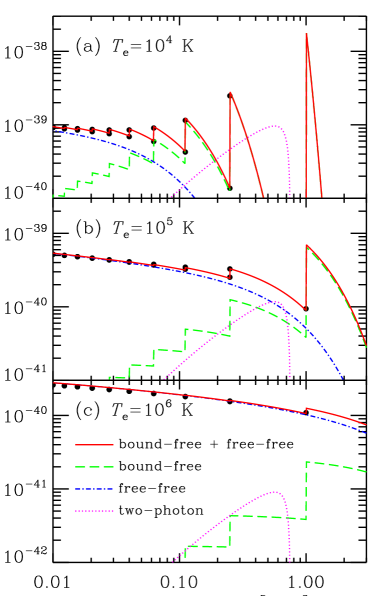
Figure 2: Hydrogen nebular emission coefficients for (a) electron temperature $T_{\rm e}=10^{4}$ K, (b) $10^{5}$ K, and (c) $10^{6}$ K. The bound-free (dashed), free-free (dot-dashed), and two-photon (dotted) coefficients are shown. The solid line in each panel is the sum of the bound-free and the free-free and it should be compared with the calculations by Ferland (1980) which are shown by small filled circles.

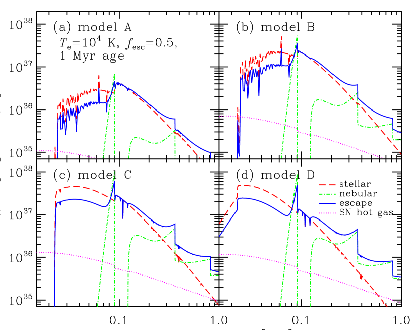
Figure 3: Spectral energy distributions (SEDs) with escaping nebular Lyman continuum: (a)–(d) for models A–D in Table 1. The assumed parameters are shown in panel (a): electron temperature $T_{\rm e}=10^{4}$ K in nebulae, escape fraction $f_{\rm esc}=0.5$, and 1 Myr after an instantaneous burst. The stellar (dashed), nebular (dot-dashed), escaping stellar+nebular (solid), and hot gas (dotted; $T_{\rm e}=10^{6}$ K and 5% of the bolometric luminosity) SEDs are shown in each panel. The vertical axis is normalized by the mass of the star cluster.

The nebular emission coefficient is the sum of three emission processes of bound-free, free-free, and two-photon as

$$\gamma^{\rm neb}_{\nu}(T_{\rm e})=\gamma^{\rm bf}_{\nu}(T_{\rm e})+\gamma^{\rm ff}_{\nu}(T_{\rm e})+\gamma^{\rm 2q}_{\nu}(T_{\rm e})\,.$$ (5)

We consider, for simplicity, nebulae composed of hydrogen only since the effect of helium is small as shown later (§4.2). The free-free and bound-free emission coefficients are calculated by equations (3) and (9) of Mewe et al. (1986). The two-photon emission coefficient is calculated as (Osterbrock & Ferland, 2006)

$$\gamma^{\rm 2q}_{\nu}=2hyP(y)X_{\rm 2q}\alpha_{\rm B}\,,$$ (6)

where $h$ is the Planck constant, $y$ is the frequency normalized by that of Ly$\alpha$, $P(y)$ is the normalized spectral shape whose approximated functional form is given by Nussbaumer & Schmutz (1984), and $X_{\rm 2q}$ is the probability of being in 2 ²S state after one Case B recombination. We adopt $X_{\rm 2q}=0.32$ (Spitzer & Greenstein, 1951). The two-photon emissivity depends on density if nebulae have a high density, but only the small density limit ($<10^{4}$ cm^-3; Osterbrock & Ferland 2006) would be enough for this paper. We also note that the Case B approximation, which is suitable for nebulae optically thick for Lyman series lines (Osterbrock & Ferland, 2006), does not conflict with our assumption of nebulae optically thin for LyC because the absorption cross sections for Lyman lines are a few orders of magnitude larger than that for LyC.

Figure 2 shows the nebular emission coefficients for $T_{\rm e}=10^{4}$, $10^{5}$, and $10^{6}$ K: bound-free (dashed lines), free-free (dot-dashed lines), and two-photon (dotted lines). We have confirmed that sums of the bound-free and free-free coefficients (solid lines) agree with the values presented in Table 1 of Ferland (1980) for $\lambda>912$ Å (small filled circles) within about 10% difference.

2.2.4 Hot gas heated by supernovae and stellar winds

In addition to photo-ionized nebulae, shock-ionized nebulae produced by multiple supernovae and stellar winds may contribute to LyC emission. According to Leitherer et al. (1999), the mechanical luminosity produced by supernovae and stellar winds is $\sim 1$% of the bolometric luminosity of stars and well less than 10% of it. We assume here 5%, a somewhat large value, to show that this component is less important. We also assume the temperature to be $10^{6}$ K for this component.

2.3 IGM attenuation

Radiation with a wavelength shorter than Ly$\alpha$ in the rest-frame of the source is absorbed by neutral hydrogen remained in the IGM. We use a Monte Carlo simulation of the IGM attenuation by Inoue & Iwata (2008). This simulation is based on an empirical distribution function of the column density, the number density, and the Doppler parameter of absorbers in the IGM which is derived from the latest observational statistics. The predicted Ly$\alpha$ decrements agree with the observations in the full range of $z=0$–6 excellently.

3 Result

3.1 Spectral energy distribution

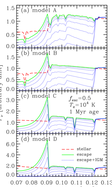
Figure 4: Close-up spectra around the Lyman limit: (a)–(d) for models A–D in Table 1. The assumed parameters are shown in panel (c): electron temperature $T_{\rm e}=10^{4}$ K in nebulae, escape fraction $f_{\rm esc}=0.5$, and 1 Myr after an instantaneous burst. The stellar (dashed) and escaping stellar+nebular (solid) spectra are the same as Figure 3. The dotted lines show spectra affected by IGM mean attenuation. Redshift of the galaxy is $z=1$ to 6 from top to bottom in each panel. The vertical axis is normalized by the flux density at Ly$\alpha$.

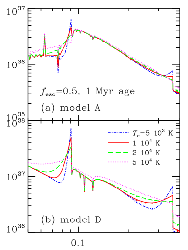
Figure 5: Effect of electron temperature $T_{\rm e}$ on the escaping SEDs: (a) for the model A and (b) for the model D. The assumed escape fraction is $f_{\rm esc}=0.5$ and the age is 1 Myr after an instantaneous burst. Four cases are shown in each panel: $T_{\rm e}=5\times 10^{3}$ K (dot-dashed), $1\times 10^{4}$ K (solid), $2\times 10^{4}$ K (dashed), and $5\times 10^{4}$ K (dotted).

First, we show the resultant SEDs without IGM attenuation in Figure 3. Panels (a)–(d) correspond to models A–D in Table 1. The assumed quantities are $T_{\rm e}=10^{4}$ K, $f_{\rm esc}=0.5$, and age of 1 Myr after an instantaneous burst. The dashed lines are the stellar SEDs. We can see that LyC becomes harder from the model A to D (see also Table 3). The dot-dashed lines are nebular emissions produced in photo-ionized nebulae. We can see bound-free Lyman, Balmer, and Paschen continua and two-photon continuum. Free-free emission is also taken into account but negligible for this case. The solid lines are escaping stellar+nebular emissions: sum of the two emissions but reduced by a factor of $f_{\rm esc}$ in LyC. We can see a significant contribution of the nebular emission. In particular, the bound-free LyC makes a bump just below the Lyman limit for models B–D. Even for the model A, the escaping LyC is a factor of 2 larger than the stellar one at $\approx 900$ Å.

The significant contribution of the nebular LyC is due to the energy re-distribution by nebulae. When a LyC photon ionizes a hydrogen atom, the photon energy moves to a photo-electron. The energy is thermalized in nebulae collisionally. Then, an electron recombines with a proton. If the recombination is to the ground state, we get a photon with an energy of 13.6 eV + kinetic energy of the electron. If $T_{\rm e}\sim 10^{4}$ K, the kinetic energy is an order of 1 eV. Thus, the photon wavelength is not far from the Lyman limit. Moreover, the recombination probability increases for an electron with a lower kinetic energy. Therefore, nebular LyC shows a peak at the Lyman limit. This is already found in the emission coefficient shown in Figure 2.

The dotted lines in Figure 3 are emissions from hot gas produced by supernovae and stellar winds. We can conclude that this component is less important On the other hand, Yajima et al. (2009) have shown an importance of shock ionization for a large escape fraction; shock ionization in addition to photo-ionization keeps the content of neutral hydrogen lower and suppresses the LyC opacity through the ISM. This is not conflict with our argument that LyC emitted by shocked gas itself is negligible.

Figure 4 shows model spectra affected by IGM attenuation (dotted lines). The assumed parameters are the same as Figure 3, and thus, the stellar (dashed) and escaping stellar+nebular spectra (solid) are the same as Figure 3. The spectra are normalized by the flux density at Ly$\alpha$ and the unit of the vertical axis is arbitrary if it is for flux density (per Hz). We can see a prominent “bump” just below the Lyman limit due to the nebular bound-free LyC. Neutral hydrogen remained in the IGM absorbs radiation below Ly$\alpha$. We apply IGM mean attenuation by Inoue & Iwata (2008) as described in §2.3.1. Each dotted line corresponds to different redshift at which the object lies: $z=1$, 2, …, 6 from top to bottom. We find that the Lyman limit bump is visible up to $z=3$ in this figure. Spectroscopic or narrowband observations tracing this wavelength range for $z\la 3$ is quite interesting to confirm the reality of the model. If the object lies along a sight-line less opaque than the average, we may find the bump from $z\approx 4$ but not from $z>5$ (see Figs. 8 and 11 in Inoue & Iwata 2008).

Figure 5 shows the effect of the assumed electron temperature $T_{\rm e}$ on the escaping stellar+nebular SEDs: $T_{\rm e}=5\times 10^{3}$ K (dot-dashed lines), $1\times 10^{4}$ K (solid), $2\times 10^{4}$ K (dashed), and $5\times 10^{4}$ K (dotted). Other parameters ($f_{\rm esc}$ and age) are the same as Figure 3. We show the models A and D only but the models B and C are qualitatively similar. We find that the shape of the Lyman limit bump becomes more peaked for lower $T_{\rm e}$. This is because the number of electrons with larger kinetic energy is smaller for lower $T_{\rm e}$ in the Maxwell-Boltzmann distribution, thus, the photon energy emitted by recombination becomes closer to the Lyman limit for lower $T_{\rm e}$. The same thing is true for the behavior around the Balmer limit.

3.2 900 Å-to-1500 Å luminosity density ratio

When estimating the escape fraction of LyC from direct observations, we often have to assume an intrinsic stellar ratio of LyC to non-ionizing UV luminosity densities (see §4 of Inoue et al., 2005). For example, Steidel, Pettini, & Adelberger (2001) assumed $L_{\nu 900}/L_{\nu 1500}=0.33$ for their $z\sim 3$ LBGs and Siana et al. (2007) argued that $L_{\nu 900}/L_{\nu 1500}=0.17$ is better for their $z\sim 1$ galaxies based on SED fitting. However, escaping stellar+nebular SEDs shown in Figure 3 are completely different from the stellar intrinsic ones because of the Lyman limit bump by the nebular bound-free LyC. Here, we present the 900 Å-to-1500 Å luminosity density ratio of escaping stellar+nebular spectra.

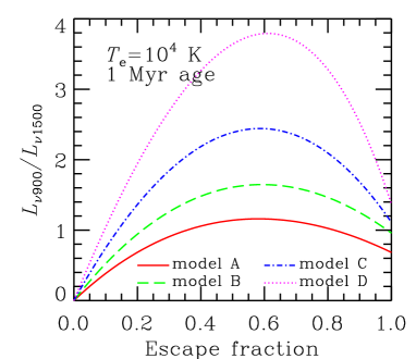
Figure 6: Luminosity density ratio (per Hz) of Lyman continuum (900 Å) to non-ionizing ultraviolet (1500 Å) as a function of escape fraction. The assumed parameters are electron temperature $T_{\rm e}=10^{4}$ K and 1 Myr after an instantaneous burst. Models A–D in Table 1 are shown with each line style.

Figure 6 shows the 900 Å-to-1500 Å luminosity density ratio as a function of escape fraction $f_{\rm esc}$ for the case with $T_{\rm e}=10^{4}$ K and 1 Myr after an instantaneous burst. Four models in Table 1 are shown by each line style: solid for model A, dashed for model B, dot-dashed for model C, and dotted for model D. At $f_{\rm esc}=1$, there is no nebula, and we see the stellar intrinsic ratio for each model. As $f_{\rm esc}$ decreases towards 0, the ratio increases, presents a peak, decreases, and reaches 0. The peak appears at $f_{\rm esc}=0.58$–0.62 and the peak ratio is a factor of 1.7–2.8 larger than the stellar ratio. Note that the 900 Å-to-1500 Å luminosity density ratio becomes maximum not when 100% of the stellar LyC escapes but when 40% of it is absorbed by nebulae. This is the Lyman bump effect due to the nebular bound-free emission.

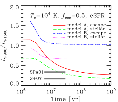
Figure 7: 900 Å-to-1500 Å luminosity density ratio (per Hz) as a function of the duration of constant star-formation for models A and B. For model A, stellar ratio is the dashed line and escaping stellar+nebular ratio is the solid line. For model B, stellar ratio is the dotted line and escaping stellar+nebular ratio is the dot-dashed line. The electron temperature $T_{\rm e}=10^{4}$ K and escape fraction $f_{\rm esc}=0.5$ are assumed. Two gray thick marks indicate the values assumed in Steidel et al. (2001, SPA01) and Siana et al. (2007, S+07).

Figure 7 shows the effect of the age on 900 Å-to-1500 Å luminosity density ratio. We again assume $T_{\rm e}=10^{4}$ K and $f_{\rm esc}=0.5$ and also assume a constant star formation for this analysis. We only show the results of the models A and B. Overall feature found in Figure 7 is that the ratio decreases after the first a few Myr and reaches an asymptotic value. This is because 900 Å radiation comes only from very massive stars whose life-time is less than a few Myr but 1500 Å radiation comes from not only such massive stars but also relatively long-lived intermediate mass stars. Thus, the 1500 Å luminosity density increases until the intermediate mass stars have turnover. The contribution of such intermediate mass stars to 1500 Å radiation depends on the IMF. For the model B, the contribution is small, and then, the luminosity density ratio reaches the asymptotic value earlier than the model A. For models C and D, the ratio is almost independent of the age because there is no intermediate mass stars in these models.

Let us compare the luminosity density ratio predicted here with those assumed in literature which are shown by gray thick marks in Figure 7. The ratio proposed by Steidel, Pettini, & Adelberger (2001) corresponds to the stellar intrinsic ratio (dashed line) for 10–20 Myr age of the model A but to the escaping stellar+nebular ratio (solid) for 100 Myr age of the model. The ratio proposed by Siana et al. (2007) corresponds to the stellar intrinsic ratio for $>100$ Myr age of the model A. On the other hand, we expect much larger ratios for younger age: $L_{\nu 900}/L_{\nu 1500}=1.1$ for the model A with the nebular contribution if age less than a few Myr. This ratio is a factor of 3 larger than Steidel, Pettini, & Adelberger (2001) and a factor of 6 larger than Siana et al. (2007). If we change the IMF (model B) or metallicity and mass range (models C and D), even larger ratios are expected (see Figure 6).

3.3 Total number of escaping LyC photons

We have seen that the 900 Å luminosity density increases due to the nebular bound-free emission. This is the radiation energy re-distribution by nebulae. How about the total number of photons in escaping LyC? The LyC photon escape rate is given by

$$Q_{\rm esc}=(Q_{*}+Q_{\rm neb})f_{\rm esc}\,,$$ (7)

with the escape fraction of stellar and nebular LyC, $f_{\rm esc}$, and the production rates of LyC photons by stars, $Q_{*}$, and by nebulae, $Q_{\rm neb}$. From the ionization equilibrium in equation (1) combined with equation (2), equation (7) is reduced to

$$\frac{Q_{\rm esc}}{Q_{*}}=\frac{\alpha_{\rm A}f_{\rm esc}}{\alpha_{\rm B}+\alpha_{1}f_{\rm esc}}\,.$$ (8)

The $Q_{\rm esc}/Q_{*}$ can be called “effective” escape fraction and depends on $f_{\rm esc}$ and $T_{\rm e}$ through $\alpha$s. Note that the escape fraction $f_{\rm esc}$ is the fraction of stellar and nebular LyC photons which escape from a galaxy relative to all (stellar+nebular) LyC photons produced in the galaxy (see eq. [7]). On the other hand, the “effective” escape fraction is the fraction of escaping stellar+nebular LyC photons relative to the photons produced by only stars.

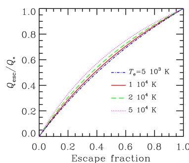
Figure 8: Ratio of the stellar+nebular escape rate to the stellar production rate of LyC photons, or “effective” escape fraction, as a function of escape fraction. Four lines show different electron temperature $T_{\rm e}$: $5\times 10^{3}$ K (dot-dashed), $1\times 10^{4}$ K (solid), $2\times 10^{4}$ K (dashed), and $5\times 10^{4}$ K (dotted).

Figure 8 shows the number fraction of LyC photons escaped relative to those produced by stars, or “effective” escape fraction, as a function of $f_{\rm esc}$ given by equation (8). The escaping number fraction is always larger than $f_{\rm esc}$ but never exceeds unity. That is, the total number of escaping LyC photons is always smaller than the number of LyC photons produced by stars. Nebular LyC compensates only a fraction of stellar LyC photons which absorbed by nebulae. Since the nebular LyC has a strong peak at the Lyman limit, however, the luminosity density near the limit is significantly enhanced as discussed in §3.2.

3.4 Mean energy of escaping Lyman continuum

Because of modification in spectra by nebular emissions, the mean energy of LyC photons escaping from galaxies is changed from that in the stellar spectrum. Let us define the mean energy of escaping LyC photons as

$$\langle\epsilon_{\rm esc}\rangle\equiv\frac{L_{\rm esc}^{\rm LyC}}{Q_{\rm esc}}=\frac{L_{*}^{\rm LyC}+L_{\rm neb}^{\rm LyC}}{Q_{*}+Q_{\rm neb}}\,,$$ (9)

where $L^{\rm LyC}$s are frequency integrated LyC luminosities of escaping, stellar, or nebular radiations. The equal is true for frequency independent $f_{\rm esc}$. The $Q$s are already introduced in equations (1) and (7). If we define mean energies of stellar and nebular LyC as $\langle\epsilon_{*}\rangle\equiv L_{*}^{\rm LyC}/Q_{*}$ and $\langle\epsilon_{\rm neb}\rangle\equiv L_{\rm neb}^{\rm LyC}/Q_{\rm neb}$, equation (9) is reduced to

$$\langle\epsilon_{\rm esc}\rangle=\beta\langle\epsilon_{*}\rangle+(1-\beta)\langle\epsilon_{\rm neb}\rangle\,,$$ (10)

where

$$\beta=\left(\frac{\alpha_{\rm B}}{\alpha_{\rm A}}\right)+\left(\frac{\alpha_{1}}{\alpha_{\rm A}}\right)f_{\rm esc}\,.$$ (11)

Note that $\langle\epsilon_{\rm neb}\rangle=\gamma_{\rm neb}^{\rm LyC}/\alpha_{1}$, where $\gamma_{\rm neb}^{\rm LyC}$ is the frequency integrated emission coefficient of nebular LyC. Therefore, the mean energy of escaping LyC is given by the internal division of mean energies of stellar and nebular LyC with weights $\beta$ and $1-\beta$, and thus, the escaping mean energy is always smaller than the stellar one if $f_{\rm esc}<1$.

Table 2: Coefficients for $\beta$ in equation (11) and mean energy of nebular Lyman continuum.

$T_{\rm e}$ ($10^{4}$ K)	$0.5$	$1$	$2$	$5$
$\alpha_{\rm B}/\alpha_{\rm A}$	$0.669$	$0.626$	$0.573$	$0.502$
$\alpha_{1}/\alpha_{\rm A}$	$0.331$	$0.374$	$0.427$	$0.498$
$\langle\epsilon_{\rm neb}\rangle$ (eV)	16.41	16.61	16.98	19.12

Table 3: Mean energies of stellar and escaping Lyman continua.

Model	A	B	C	D
$\langle\epsilon_{*}\rangle$ (eV)	22.66	23.00	26.85	32.18
$\langle\epsilon_{\rm esc}\rangle$ (eV)a	21.53	21.81	24.94	29.27
$\langle\epsilon_{\rm esc}\rangle$ (eV)b	20.62	20.85	23.40	26.93

^a $T_{\rm e}=10^{4}$ K, $f_{\rm esc}=0.5$

^b $T_{\rm e}=10^{4}$ K, $f_{\rm esc}=0.1$

In Table 2 we summarize the coefficients for $\beta$ in equation (11) and the mean photon energy of nebular LyC as a function of $T_{\rm e}$. Table 3 gives a summary of mean photon energies of stellar LyC for models A–D in the first row. The second and third rows in Table 3 show mean photon energies of escaping stellar+nebular LyC for two cases of $T_{\rm e}=10^{4}$ K and $f_{\rm esc}=0.5$ or 0.1. We find that the energy reduction is about 5–15% for these cases and its maximum is 10–20% at the limit of $f_{\rm esc}\to 0$.

4 Discussion

4.1 Wavelength dependent opacity and comparison with the code Cloudy

As described in §2.2.1, LyC opacity through a clumpy ISM is independent of wavelength. As an opposite limit, we here consider a homogeneous ISM where the opacity keeps the wavelength dependence of the photo-ionization cross section of hydrogen: $\propto\lambda^{3}$.

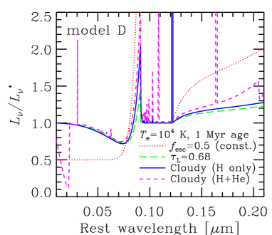
Figure 9: Spectra relative to the stellar one and comparison with results from Cloudy. The electron temperature $T_{\rm e}=10^{4}$ K and the age of 1 Myr after an instantaneous burst for the stellar population model D are assumed. The dotted line is the escaping stellar+nebular spectrum with a constant escape fraction $f_{\rm esc}=0.5$ which is the same as in Figures 3 and 4. The long-dashed line is the escaping stellar+nebular spectra for which we assume the neutral hydrogen optical depth at the Lyman limit $\tau_{\rm L}=0.68$ and at shorter wavelengths to be $\propto\lambda^{3}$. The solid and short-dashed lines are the cases calculated with Cloudy 08.00 (Ferland et al. 1998) for hydrogen only case and hydrogen and helium case, respectively. The Lyman limit optical depth for the hydrogen only case is matched to 0.68.

Figure 9 shows escaping stellar+nebular spectra relative to the stellar one in a homogeneous ISM (LyC opacity depends on the cube of wavelength) for the model D. The Lyman limit optical depth is set to be 0.68. This opacity corresponds to $f_{\rm esc}=0.5$ at the Lyman limit and is applied to both stellar and nebular LyC (long-dashed line). If we compare the case in a clumpy ISM presented in the previous sections (dotted line), we find that the Lyman limit bump predicted in a homogeneous ISM is weaker than that in a clumpy ISM. This is because higher energy LyC escapes easily and does not convert to nebular emission in the wavelength dependent case (i.e. homogeneous ISM). To make a strong bump, we need to convert higher energy LyC to the Lyman limit by clumpy nebulae.

We can use the public photo-ionization code, Cloudy (Ferland et al., 1998) for a homogeneous ISM. To check our nebular calculations, we compare our results with the code Cloudy in Figure 9. We input the following condition to the code: a point source with the production rate of hydrogen LyC photons of $10^{52.01}$ s^-1, which corresponds to $10^{4}$ $M_{\odot}$ in the stellar mass for the model D, resides at the center of spherical symmetric gas with the hydrogen atomic number density of 1 cm^-3 and with the temperature of $10^{4}$ K. We set the inner and outer boundaries to be $10^{20}$ cm and $10^{21}$ cm, respectively. The outer boundary is determined to achieve a Lyman limit optical depth of 0.68. This case is shown by the solid line in Figure 9. We find a good agreement between our calculation (long-dashed) and Cloudy (solid). However, Cloudy predicts somewhat stronger bump at the Lyman limit. This is because the optical depth for nebular LyC is smaller than that for stellar one since the nebula surrounds the source, whereas we set the same optical depth for both continua.

The short-dashed line in Figure 9 is the case where the spherical gas consists of hydrogen and helium. Other settings are the same as the hydrogen only case. The resultant continuum is not very different from the hydrogen only case. Thus, the effect of helium is small for the shape of the SED. This point is also discussed in the next subsection.

4.2 Effect of helium

We can derive equations for helium nebular emissions like equation (4) for hydrogen. The strength of the helium emissions relative to that of hydrogen can be approximated to

$$\frac{L_{\nu}^{X}}{L_{\nu}^{\rm H}}\approx\left(\frac{\gamma_{\nu}^{X}}{\gamma_{\nu}^{\rm H}}\right)\left(\frac{Q_{*}^{X}}{Q_{*}^{\rm H}}\right)\left(\frac{\alpha_{\rm B}^{\rm H}}{\alpha_{\rm B}^{X}}\right)\,,$$ (12)

where $X$ is neutral helium (He I) or singly ionized helium (He II) and other quantities have the same meanings as in §2 but with superscript describing which atom or ion. In the four models of A–D considered here, we found $Q_{*}^{\rm HeI}/Q_{*}^{\rm HI}=0.4$–0.7 and $Q_{*}^{\rm HeII}/Q_{*}^{\rm HI}=4\times 10^{-4}$–0.1 with a larger value for a smaller metallicity (Schaerer, 2002, 2003). The recombination rates of helium are $\alpha_{\rm B}^{\rm HeI}\approx\alpha_{\rm B}^{\rm HI}$ and $\alpha_{\rm B}^{\rm HeII}\approx 4\alpha_{\rm B}^{\rm HI}$ (Osterbrock & Ferland, 2006). According to the emission coefficients shown in Osterbrock & Ferland (2006), we found that the helium contribution is negligible in the wavelength range of 800–2000 Å, except for the model D where the He II bound-free Paschen continuum contributes about 20% around 2000 Å. This smallness of the effect of helium on continuum can be confirmed in Figure 9 if we look at the result by Cloudy with hydrogen and helium (short-dashed line). However, the effect on recombination lines may not be negligible.

4.3 Lyman “bump” as a tool to find exotic stellar populations

As shown in Figure 4, we predict that galaxies dominated by very young ($\sim 1$ Myr) and massive stellar populations can have a Lyman limit “bump” not “break” expected in the stellar spectra. The strength of the bump depends on the hardness of the LyC (see also Figure 6). If galaxies contain very massive ($\sim 100$ $M_{\odot}$) EMP stars or metal-free (Pop-III) stars, the Lyman limit bump becomes very strong. This fact provides a new method to find such exotic stellar populations in galaxies at $z\la 4$ although the IGM attenuation hampers us to use this method for galaxies at $z>4$. Indeed, Iwata et al. (2009) have found very interesting LAEs at $z=3.1$ which emit extremely strong LyC. We will apply the model developed in this paper to the LAEs in the forthcoming paper and discuss their nature in detail.

4.4 Effect on reionization

Let us examine if escaping nebular LyC affects the reionization process. The reionization history is regulated by the product of escape fraction and star formation efficiency, $f_{\rm esc}f_{*}$, if we assume a cosmological structure formation scenario (Wyithe & Loeb, 2003). As the first effect of escaping nebular LyC, this $f_{\rm esc}$ should be replaced by “effective” escape fraction, $Q_{\rm esc}/Q_{*}$, which is introduced in equation (8) and Figure 8. From equations (8) and (11), we obtain $Q_{\rm esc}/Q_{*}=f_{\rm esc}/\beta$ and find that the “effective” escape fraction is at most a factor of 1.6 larger than $f_{\rm esc}$ for $T_{\rm e}=10^{4}$ K. As the second effect, the nebular LyC modifies the LyC spectral shape and reduces the mean photon energy of escaping LyC. This leads to a decrease of the mean free path of LyC photons in the IGM. However, the reduction of the mean photon energy is at most 10–20% relative to that of the stellar LyC as discussed in §3.4 and in Tables 2 and 3. Therefore, the nebular LyC escape itself may not give a significant impact on the reionization process.

5 Conclusion

The discovery of $z=3.1$ LAEs emitting extremely strong LyC by the Subaru telescope (Iwata et al., 2009) requires us to examine LyC emissivity and spectrum of galaxies more carefully. As an attempt, this paper has examined the effect of an escape of nebular LyC on SEDs of galaxies. The nebular LyC mainly emitted by bound-free transitions of hydrogen is usually assumed to be absorbed within nebulae, so-called “on-the-spot” approximation (Osterbrock & Ferland, 2006). However, we should consider its escape if stellar LyC escapes from galaxies as observed at $z\sim 3$ (Steidel, Pettini, & Adelberger, 2001; Shapley et al., 2006; Iwata et al., 2009).

Since the bound-free nebular emission has strong peaks at the limits of Lyman, Balmer, Paschen, etc. (see Figure 2), we expect a bump at the Lyman limit due to escaping nebular bound-free LyC (see Figure 3). This bump boosts luminosity density at 900 Å. As a result, 900 Å-to-1500 Å luminosity density ratio can become larger than that expected in stellar SEDs. Indeed, the ratio has a maximum not when $f_{\rm esc}=1$ but when $f_{\rm esc}=0.6$ (see Figure 6). The strength of the bump depends on $T_{\rm e}$ in nebulae (see Figure 5), hardness of stellar LyC (i.e. metallicity, IMF and mass range, and age; see Figures 3 and 7), and IGM attenuation (see Figure 4). On the other hand, the total number of LyC photons which escape from galaxies is always less than that produced by stars (see Figure 8). In fact, the Lyman limit bump is a result of the radiation energy re-distribution by nebulae. The energy re-distribution reduces the mean energy of escaping LyC photons, but it is at most 10–20% reduction relative to the mean energy of stellar LyC (see Table 3).

We have assumed wavelength independent $f_{\rm esc}$ (or LyC opacity through the ISM) to obtain our main results. This should be suitable for a clumpy ISM (see schematic Figure 1 and discussion in §2.2.1). We have also calculated a wavelength dependent case which corresponds to a homogeneous ISM, and have found that the wavelength dependent case predicts a weaker Lyman limit bump (see Figure 9). In addition, we have compared the case with the photo-ionization code Cloudy (Ferland et al., 1998), and have found a good agreement (see Figure 9). Moreover, we have omitted helium, but it is justified by a discussion in §4.2 and by a comparison with Cloudy (see Figure 9).

The most interesting implication from our results would be the prediction of Lyman “bump” galaxies (see Figure 4 and §4.3); galaxies containing very young ($\sim 1$ Myr), very massive ($\sim 100$ $M_{\odot}$), and extremely metal-poor (or metal-free) stellar populations show a prominent bump just below the Lyman limit. This would be a new indicator to find such exotic stellar populations. Although IGM attenuation hampers us to use this method for $z>5$ galaxies, we can use it for $z<4$ galaxies.

Finally, we have discussed effects on the reionization briefly (§4.4). Escaping nebular LyC has two effects: acting as an additional LyC source and reducing the mean energy of escaping LyC photons. The first effect increases the escape fraction effectively, but the enhancement is at most a factor of 1.6 (for $T_{\rm e}=10^{4}$ K) and the LyC photon escape rate never exceeds the production rate by stars (see Figure 8). The second effect decreases the mean free path of LyC photons in the IGM. However, the reduction of the mean photon energy is at most 10–20% relative to the stellar LyC (see Table 3). Therefore, the nebular effect on the reionization may be small.

References

- Becker et al. (2001) Becker, R. H., Fan, X., White, R. L., Strauss, M. A., Narayanan, V. K., Lupton, R. H., Gunn, J. E., Annis, J., Bahcall, N. A., et al., 2001, AJ, 122, 2850
- Beers & Christlieb (2005) Beers, T. C., Christlieb, N., 2005, ARA&A, 43, 531
- Bergvall et al. (2006) Bergvall, N., Zackrisson, E., Andersson, B.-G., Arnberg, D., Masegosa, J., Östlin, G., 2006, A&A, 448, 513
- Cowie, Barger, & Trouille (2009) Cowie, L. L., Barger, A. J., & Trouille, L., 2009, ApJ, 692, 1476
- Deharveng et al. (2001) Deharveng, J.-M., Buat, V., Le Brun, V., Milliard, B., Kunth, D., Shull, J. M., Gry, C., 2001, A&A, 375, 805
- Fan, Carilli, Keating (2006) Fan, X., Carilli, C. L., Keating, B., 2006, ARA&A, 44, 415
- Ferland (1980) Ferland, G. J., 1980, PASP, 92, 596
- Ferland et al. (1998) Ferland, G. J., Korista, K. T., Verner, D. A., Ferguson, J. W., Kingdon, J. B., Verner, E. M., 1998, PASP, 110, 761
- Grimes et al. (2007) Grimes, J. P., Heckman, T., Strickland, D., Dixon, W. V., Sembach, K., Overzier, R., Hoopes, C., Aloisi, A., et al., 2007, ApJ, 668, 891
- Hurwitz, Jelinsky, & Dixon (1997) Hurwitz, M., Jelinsky, P., Dixon, W. V. D., 1997, ApJ, 481, L31
- Inoue et al. (2005) Inoue, A. K., Iwata, I., Deharveng, J.-M., Buat, V., Burgarella, D., 2005, A&A, 435, 471
- Inoue, Iwata, & Deharveng (2006) Inoue, A. K., Iwata, I., Deharveng, J.-M., 2006, MNRAS, 371, L1
- Inoue & Iwata (2008) Inoue, A. K., Iwata, I., 2008, MNRAS, 387, 1681
- Iwata et al. (2009) Iwata, I., Inoue, A. K., Matsuda, Y., Furusawa, H., Hayashino, T., Kousai, K., Akiyama, M., Yamada, T., et al., 2009, ApJ, 692, 1287
- Iye et al. (2006) Iye, M., Ota, K., Kashikawa, N., Furusawa, H., Hashimoto, T., Hattori, T., Matsuda, Y., Morokuma, T., Ouchi, M., et al., 2006, Nature, 443, 186
- Kashikawa et al. (2006) Kashikawa, N., Shimasaku, K., Malkan, M. A., Doi, M., Matsuda, Y., Ouchi, M., Taniguchi, Y., Ly, C., et al., 2006, ApJ, 648, 7
- Leitherer et al. (1995) Leitherer, C., Ferguson, H. C., Heckman, T. M., Lowenthal, J. D., 1995, ApJ, 454, L19
- Leitherer et al. (1999) Leitherer, C., Schaerer, D., Goldader, J. D., González-Delgado, R. M., Robert, C., Kune, D. F., de Mello, D. F., Devost, D., et al., 1999, ApJS, 123, 3
- Madau, Meiksin, & Rees (1997) Madau, P., Meiksin, A., Rees, M. J., 1997, ApJ, 475, 429
- Madau, Haardt, & Rees (1999) Madau, P., Haardt, F., Rees, M. J., 1999, ApJ, 514, 648
- Mewe et al. (1986) Mewe, R., Lemen, J. R., van den Oord, G. H. J., 1986, A&AS, 65, 511
- Moy, Rocca-Volmerange, Fioc (2001) Moy, E., Rocca-Volmerange, B., Fioc, M., 2001, A&A, 365, 347
- Myers (1978) Myers, P. C., 1978, ApJ, 225, 380
- Nussbaumer & Schmutz (1984) Nussbaumer, H., Schmutz, W., 1984, A&A, 138, 495
- Osterbrock & Ferland (2006) Osterbrock, D. E., Ferland, G. J., 2006, Astrophysics of gaseous nebulae and active galactic nuclei, 2nd. ed., University Science Books, Sausalito, CA.
- Razoumov & Sommer-Larsen (2006) Razoumov, A. O., Sommer-Larsen, J., 2006, ApJ, 651, 89
- Razoumov & Sommer-Larsen (2007) Razoumov, A. O., Sommer-Larsen, J., 2007, ApJ, 668, 674
- Salpeter (1955) Salpeter, E. E., 1955, ApJ, 121, 161
- Salvaterra et al. (2009) Salvaterra, R., Della Valle, M., Campana, S., Chincarini, G., Covino, S., D’Avanzo, P., Fernandez-Soto, A., Guidorzi, C., et al. 2009, arXiv:0906.1578
- Schaerer (2002) Schaerer, D., 2002, A&A, 382, 28
- Schaerer (2003) Schaerer, D., 2003, A&A, 397, 527
- Schaerer & de Barros (2009) Schaerer, D., de Barros, S., 2009, A&A, 502, 423
- Shapley et al. (2006) Shapley, A. E., Steidel, C. C., Pettini, M., Adelberger, K. L., Erb, D. K., 2006, ApJ, 651, 688
- Siana et al. (2007) Siana, B., Teplitz, H. I., Colbert, J., Ferguson, H. C., Dickinson, M., Brown, T. M., Conselice, C. J., de Mello, D. F., et al., 2007, ApJ, 668, 62
- Spitzer & Greenstein (1951) Spitzer, L. Jr., Greenstein, J. L., 1951, ApJ, 114, 407
- Stasínska & Leitherer (1996) Stasínska, G., Leitherer, C., 1996, ApJS, 107, 661
- Steidel, Pettini, & Adelberger (2001) Steidel, C. C., Pettini, M., Adelberger, K. L., 2001, ApJ, 546, 665
- Tanvir et al. (2009) Tanvir, N. R., Fox, D. B., Levan, A. J., Berger, E., Wiersema, K., Fynbo, J. P. U., Cucchiara, A., Kruehler, T., et al., 2009, arXiv:0906.1577
- Totani et al. (2006) Totani, T., Kawai, N., Kosugi, G., Aoki, K., Yamada, T., Iye, M., Ohta, K., Hattori, T., 2006, PASJ, 58, 485
- Vázquez et al. (2007) Vázquez, G. A., Leitherer, C., Schaerer, D., Meynet, G., Maeder, A., 2007, ApJ, 663, 995
- Wyithe & Loeb (2003) Wyithe, J. S. B., Loeb, A., 2003, ApJ, 586, 693
- Yajima et al. (2009) Yajima, H., Umemura, M., Mori, M., Nakamoto, T., 2009, MNRAS, in press (arXiv:0906.1658)
- Zackrisson et al. (2001) Zackrisson, E., Bergvall, N., Olofsson, K., Siebert, A., 2001, A&A, 375, 814
- Zackrisson, Bergvall, & Leitet (2008) Zackrisson, E., Bergvall, N., Leitet, E., 2008, ApJ, 676, L9