Time evolution of spin-boson system for different effective spectral density functions

Abstract

In this paper we firstly obtain two kinds of effective spectral density functions by setting the cut-off frequencies of baths be infinite and finite. Secondly, we investigate the reduced dynamics of open qubits in four kinds of systems constructed with the basic spin-boson model. It is shown that the qubit has different dynamics governed by the two kinds of spectral density functions. In addition, we obtained that a qubit coupled to an intermediate harmonic oscillator has longer decoherence and relaxation times as they are coupled to a common bath than to their respective baths. In solving the dynamics of qubits we use a numerically exact algorithm, iterative tensor multiplication algorithm based on the quasiadiabatic propagator path integral scheme.

LABEL:FirstPage1 LABEL:LastPage#1102

I Introduction

As a quantum system of interest interacts with its environment which is also considered being made up of a large number of the quantum particles, solving the dynamics of the total system is in fact an impossible task by now. However, in many cases we are only interested in the dynamics of the quantum system of interest, thus we can investigate the reduced system by using the phenomenological environment as proposed by Caldeira and Leggett AnnPhys149_374_1983 . Usually, in this method the environment is modelled by a bath of harmonic oscillators (or other quantum particles) and the influence of the bath on the quantum system is fully enclosed in the so-called spectral density function $J(\omega).$ According to the characteristic of the environment one can choose the $J(\omega)$ Ohmic, sub-Ohmic, super-Ohmic forms and so on. Thus, the reduced dynamics of the quantum systems can be investigated in detail. Many such problems have been treated extensively and some significative results have been obtained in the field in past years Weiss-book ; RMP59_1_1987 .

The spectral density functions $J(\omega)$ obtained from the microcosmic dynamical model plus its phenomenological environment (MDMPPE) is in good agreement with that obtained from quasi-classical equations of motion satisfied by the system of interest. We can obtain the effective spectral density function (ESDF) following Leggett as follows. Setting $\sum_{i}c_{i}^{2}\delta\left(\omega-\omega_{i}\right)/m_{i}\omega_{i}=J_{0}(\omega),$ taking cut-off frequency of the bath modes infinity, and supposing the spectral density function $J(\omega)$ a continuous function, we can obtain the ESDF with $J(\omega)=$Im$[K(\omega)]$ (see Ref.PRB30_1208_1984 ), where $K(\omega)$ represents the effects of arbitrary linear dissipative and/or reactive elements. Usually, $K(\omega)$ can be obtained from the equation of motion of the system in Fourier-transformed form, namely, $K(\omega)q\left(\omega\right)=-\left[\partial V\left(q\right)/\partial q\right]\left(\omega\right),$ where $V\left(q\right)$ is a conservative potential. This equation can be obtained from the scheme of MDMPPE. The ESDFs from infinite cut-off frequency of baths for many models are obtained JCP83_4491_1985 ; PhysRep168_115_1988 ; CPL449_296_2007 . This method is in fact a universal one.

However, when the temperature of the systems are low enough, we can imagine that the dynamics of the quantum systems of interest obtained from the MDMPPE should have some difference with that from quasi-classical equations of motions. In this case, the high-frequency modes of the bath are in fact suppressed, so the cut-off frequency may be not very large and it may be comparable to the characteristic frequency of the quantum system of interest. So there are at least two differences between the dynamics of normal and low temperature for the quantum systems of interest. The first is that the ESDFs obtained from the MDMPPE at low temperature should not be in accordance with the spectral density functions from quasi-classical equations of motion, and the second is that the system at low temperature must go through a non-Markovian process PRB78_235311_2008 ; JCP129_224106_2008 other than the Markovian one.

With the progress of technique many quantum systems have been designed and manufactured. In particular, many qubit models for making quantum computers in future are proposed in recent years. Most of these quantum systems should work in very low temperature PRB75_104516_2007 ; PRB76_155323_2007 . The non-Markovian effects of baths in the systems have been considered recently PRA80_042112_2009 ; PRE80_041106_2009 ; PRA80_031143_2009 ; PRL103_050403_2009 . It is reported that in many chemical and biologic systems, the non-Markovian effects may also be important ChemRev109_2350_2009 ; CP347_185_2008 ; Science316_1462_2007 ; Nature446_782_2007 . At very low temperature, the cut-off frequencies of the bath should be finite. Taking a finite cut-off frequency of the bath rather than the infinite one, we shall obtain another kind of the spectral density function. In the following we denote the ESDFs from infinite, and from finite cut-off frequencies of the bath for model $x$ by $J_{x}^{I}(\omega)$ (from infinite cut-off frequencies) and $J_{x}^{F}(\omega)$ (from finite cut-off frequencies), where $x$ denotes the physical models. A somewhat similar discussion on the problem in completely classical framework has been given in Refs EPJB61_271_2008 ; PRE79_031128_2009 .

In this paper, we shall investigate the ESDFs of four models by using the scheme of MDMPPE at infinite and finite cut-off frequencies of baths. Through the two sets of ESDFs $J_{x}^{I}\left(\omega\right)\$ and $J_{x}^{F}\left(\omega\right)$ we shall investigate the reduced dynamics of qubits in some practical physical models. They are a quantum system in a bath (model A); a quantum system coupled to an intermediate harmonic oscillator (IHO) and only the latter coupled to a bath (model B); a quantum system coupled to an IHO and both of them coupled to their independent baths (model C) and a common bath (model D).

II Two kinds of spectral density functions and the dynamics of open qubits

In this section, we shall obtain two kinds of ESDFs for the models A, B, C, and D when they are reduced to the original spin-boson form. One kind of them are obtained from taking finite cut-off frequencies of baths and the other is gotten by setting the cut-off frequencies of baths infinity. After obtaining the spectral density functions we shall solve the reduced dynamics for the quantum systems of interest when they are set as the qubits. The reduced dynamics governed by the two kinds of ESDFs for the qubits will be compared.

In order to compare the dynamics of the qubit governed by the different effective spectral functions in each model, we choose a same starting point $J_{0}\left(\omega\right)$ for all of the models. In another word, we always reduce them to the original spin-boson model with the same IHO transformation and set $J_{0}(\omega)=\sum_{i}c_{i}^{2}\delta\left(\omega-\omega_{i}\right)/m_{i}\omega_{i}=\eta\omega e^{-\omega/\omega_{c}}$ in our derivations. Because the model A is just the original spin-boson model, our work for reducing this model is just reducing it to itself. So in the assumption of infinite cut-off frequency, the obtained ESDF of the model should be equal to the $J_{0}\left(\omega\right)$, which will be shown in the following subsection A. Models B, C, and D are different from the original spin-boson model, so when they are reduced to the original spin-boson form, the ESDFs should be different from the starting function $J_{0}\left(\omega\right)$.

We have calculated the dynamics of the quantum system of interest governed by $J_{x}^{I}\left(\omega\right)$ and $J_{x}^{F}\left(\omega\right)$ with the same values of $\eta$ in each models of the paper, and they are certainly different. However, even for the same model, the different ESDFs $J_{x}^{I}\left(\omega\right)$ and $J_{x}^{F}\left(\omega\right)$, may provide different damping for the same $\eta$ in the function $J_{0}(\omega)$, which will affect the dynamics of the quantum system of interest. Do the different kinds ESDFs affect the dynamics of quantum system of interest mainly through resulting in different damping or through their different forms? To answer this problem, we introduce an effective coupling strength $\eta^{\prime}=J(\omega=\omega_{0})/\omega_{0}$ to calculate the dynamics as Ref.JCP96_8485_1992 . The effective coupling constant is introduced from the physical deduce that the modes which has the same frequency as the characteristic frequency of the system $\omega_{0}$ has the major contribution to the system-bath interaction. Thus, by using the effective coupling constant we can obtain that, if the reduced dynamics governed by $J_{x}^{I}\left(\omega\right)$ and $J_{x}^{F}\left(\omega\right)$ are different, we can safely attribute the different forms of the $J_{x}^{I}\left(\omega\right)$ and $J_{x}^{F}\left(\omega\right)$. For lack of space, in the following, we only plot the evolutions of elements of reduced density matrix in the same effective coupling strength $\eta^{\prime}$ for each models.

II.1 Two basic models (models A and B)

A quantum system embeds in a bath (model A) and a quantum system interacts with an IHO which is coupled to a bath (model B), are two basic models and many complicated models are developed from them. So in this subsection, we use them to show the Leggett’s method for obtaining the ESDFs $J_{A/B}^{I}\left(\omega\right)$, and $J_{A/B}^{F}\left(\omega\right)$. Then from the two sets of ESDFs we investigate the reduced dynamics of qubits in the two models.

Model A: Because the physical quantities of the quantum system of interest is not included in the ESDF, we can deduce the ESDFs of the model A with the Hamiltonian as JCP83_4491_1985

$$H_{A}=\frac{p_{q}^{2}}{2\mu}+U\left(q\right)+{\textstyle\sum_{i}}\frac{p_{i}^{2}}{2m_{i}}+\frac{1}{2}m_{i}\omega_{i}^{2}\left(x_{i}+\frac{c_{i}q}{m_{i}\omega_{i}^{2}}\right)^{2},$$ (1)

where $p_{q}$ is the momentum conjugate to coordinate $q$. Defining $U^{\prime}=dU/dt$ and using the dots for the time derivatives, we can obtain the classical equations of the motion as

$$\mu\ddot{q} =-U^{\prime}(q)-{\textstyle\sum_{i}}c_{i}x_{i}-{\textstyle\sum_{i}}\frac{c_{i}^{2}q}{m_{i}\omega_{i}^{2}},$$ (2)

$$m_{i}\ddot{x}_{i} =-m_{i}\omega_{i}^{2}x_{i}-c_{i}q.$$ (3)

Using the Fourier transforms, we can write Eqs.(2) and (3) as

$$-\mu\omega^{2}q\left(\omega\right) =-U_{\omega}^{\prime}(q\left(t\right))-{\textstyle\sum_{i}}c_{i}x_{i}\left(\omega\right)-{\textstyle\sum_{i}}\frac{c_{i}^{2}q\left(\omega\right)}{m_{i}\omega_{i}^{2}},$$ (4)

$$-m_{i}\omega^{2}x_{i}\left(\omega\right) =-m_{i}\omega_{i}^{2}x_{i}\left(\omega\right)-c_{i}q\left(\omega\right).$$ (5)

From Eq.(5) we have

$$x_{i}\left(\omega\right)=-\frac{c_{i}}{m_{i}\left(\omega_{i}^{2}-\omega^{2}\right)}q\left(\omega\right),$$ (6)

Insetting Eq.(6) into Eq.(4), we have

$$\left[-\mu\omega^{2}-\omega^{2}{\textstyle\sum_{i}}\frac{c_{i}^{2}}{m_{i}\omega_{i}^{2}\left(\omega_{i}^{2}-\omega^{2}\right)}\right]q(\omega)=-U_{\omega}^{\prime}(q\left(t\right)).$$ (7)

Setting

$$L\left(\omega\right)={\textstyle\sum_{i}}\frac{c_{i}^{2}}{m_{i}\omega_{i}^{2}\left(\omega_{i}^{2}-\omega^{2}\right)},$$ (8)

and

$$J_{0}\left(\omega^{\prime}\right)=\pi\sum\frac{c_{i}^{2}}{m_{i}\omega_{i}}\delta\left(\omega^{\prime}-\omega_{i}\right)\equiv\omega^{\prime}\eta e^{-\omega^{\prime}/\omega c},$$ (9)

we then have

$$L\left(\omega\right) =\frac{1}{\pi}\int_{0}^{\infty}\frac{J_{0}\left(\omega^{\prime}\right)}{\omega^{\prime}\left(\omega^{\prime 2}-\omega^{2}\right)}d\omega^{\prime}$$

$$=\frac{1}{\pi}\eta\int_{0}^{\infty}\frac{\exp(-\omega^{\prime}/\omega_{c})}{\left(\omega^{\prime 2}-\omega^{2}\right)}d\omega^{\prime}\equiv\frac{1}{\pi}\eta R\left(\omega\right),$$ (10)

where (see Appendix)

$$R\left(\omega\right)=-\frac{\pi i}{\omega}e^{-\omega/\omega c}-\frac{\pi}{\omega}W\left(\omega\right).$$ (11)

The expression of $W\left(\omega\right)$ is given in the Appendix. Substituting Eq.(11) into Eq.(7) we have

$$K\left(\omega\right)q\left(\omega\right) =\left[-\mu\omega^{2}+\omega\eta W\left(\omega\right)+\omega\eta ie^{-\omega/\omega c}\right]q\left(\omega\right)$$

$$=-U_{\omega}^{\prime}\left(q\right).$$ (12)

If taking $\omega_{c}$ be infinite, we can easily obtain the spectral density function as

$$J_{A}^{I}\left(\omega\right)=\omega\eta e^{-\omega/\omega c}.$$ (13)

This is the conventional Ohmic spectral density function of bath in the original spin-boson model and it has been widely used in quantum dissipative systems. Here, we have only shown that, starting from $J_{0}\left(\omega\right)$, an ESDF $J_{A}^{I}\left(\omega\right)$ can be obtained. The $J_{0}\left(\omega\right)$ and $J_{A}^{I}\left(\omega\right)$ are the same for the bath in the original spin-boson model. The result shows that the Leggett’s method give a consistent result for the model. If the model is not the original spin-boson model (as following models B, C, and D), it can also be reduced to the original spin-boson model but the ESDFs should not be equal to the $J_{0}\left(\omega\right)$ even we start from the same $J_{0}\left(\omega\right)$.

If taking $\omega_{c}$ be finite, we then obtain the ESDF as

$$J_{A}^{F}(\omega)=\operatorname{Im}(K(\omega))=\omega\eta\Theta\left(\omega\right).$$ (14)

Here, $\Theta\left(\omega\right)=\operatorname{Im}\left(W\left(\omega\right)\right)+e^{-\omega/\omega_{c}}.$ The other forms of the spectral density functions, such as sub-Ohmic and super-Ohmic forms can be obtained similarly. It shows that when the cut-off frequency is finite, we should add the term $\eta\omega\operatorname{Im}[W\left(\omega\right)]$ in the spectral density function as Eq.(14). It is interesting that how does the added term influence the spectral density function? In Fig.1 we plot $\operatorname{Im}[W\left(\omega\right)]$ in different cut-off frequencies of the bath. It shows that the absolute values of the $\operatorname{Im}[W\left(\omega\right)]$ decreases with the increase of $\omega_{c}$. When $\omega_{c}\rightarrow\infty$, the $\operatorname{Im}[W\left(\omega\right)]\rightarrow 0$. However, when the cut-off frequency of the bath is not big enough, the influence of $\operatorname{Im}[W\left(\omega\right)]$ should not be neglected in the description of the environment.

In above derivation of the ESDFs, the physical quantities for the quantum system of interest have not been involved, so the $J\left(\omega\right)$ can control the dynamics of not only the harmonic oscillator as in Eq.(1) but also other quantum systems. In order to check the differences of the influences that above two different ESDFs $J_{A}^{I}\left(\omega\right)$ and $J_{A}^{F}\left(\omega\right)$ impose on the dynamics for the systems of interest, we firstly investigate a simple quantum system, qubit. For the open qubit the total Harmiltonian reads

$$H=\frac{\hbar}{2}\left(\epsilon\sigma_{z}+\Delta\sigma_{x}\right)+{\textstyle\sum_{i}}\frac{p_{i}^{2}}{2m_{i}}+\frac{1}{2}m_{i}\omega_{i}^{2}\left(x_{i}+\frac{c_{i}\sigma_{z}}{m_{i}\omega_{i}^{2}}\right)^{2}.$$ (15)

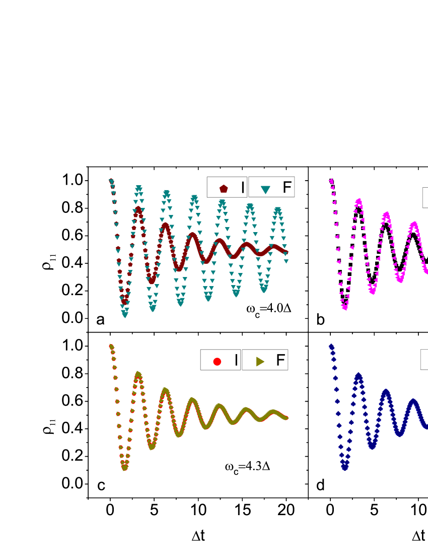
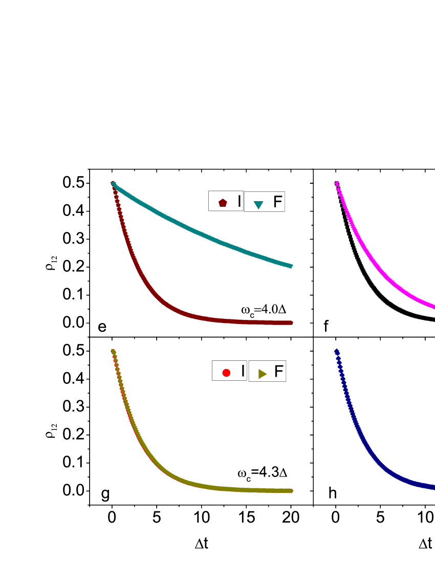
Figure 2: (Color online) The reduced dynamics of qubit governed by $J_{A}^{I}\left(\omega\right)$ vs by $J_{A}^{F}\left(\omega\right)$ in different values of $\omega_{c}$. Top four figures a, b, c, and d plot the evolutions of the diagonal element $\rho_{11}(t)$ beginning at the initial state $\rho_{1}(0)$, where $\Delta=10^{12}$ Hz, $\epsilon=0.01\Delta$. Bottom four figures e, f, g, and h plot the evolutions of off-diagonal element $\rho_{12}(t)$ beginning at the initial state $\rho_{2}(0)$, where $\epsilon=10^{12}$ Hz, $\Delta=0.01\epsilon$, T=300 k, $\eta^{\prime}=0.004$. The $\rho_{1}(0)$ and $\rho_{2}(0)$ are supposed in the text. Here, and in the following, we denote the results from the ESDFs $J^{I}(\omega)$, and $J^{F}(\omega)$ with I and F in the Legend

This is one of the simplest open models of quantum system but its reduced dynamics can still not be solved exactly, and some approximations must be appealed to. Many investigations on this topic have been made in recent years JCP126_114102_2007 ; JCP130_164518_2009 ; JCP130_204512_2009 ; JPSJ75_082001_2006 ; JPSJ78_073802_2009 . As we stressed that when the cut-off frequency is not too large to compare to the characteristic frequency of the qubit, the non-Markovian effect is non-negligible. The well established iterative tensor multiplication (ITM) algorithm based on the quasiadiabatic propagator path integral (QUAPI) scheme is a good tool for solving the reduced dynamics of quantum system of interest. The ITM algorithm is a numerically exact one and is successfully tested and adopted in various problems of open quantum systems JCP102_4600_1995 ; CPL221_482_1994 ; PNAS93_3926_1996 ; PRE62_5808_2000 ; PRB72_245328_2005 . For details of the scheme, we refer readers to previous works JCP102_4600_1995 ; CPL221_482_1994 ; PNAS93_3926_1996 ; PRE62_5808_2000 ; PRB72_245328_2005 . To make the calculations converge we use the time step $\delta t=0.1/\Delta$ which is shorter than the correlation time of the bath and the characteristic time of the qubit. In order to include as much non-Markovian effect of the bath as we can, and avoid the heavy calculation load we choose $\delta k_{\max}=3$. Here, $\delta k_{\max}\times\delta t$ is the memory times being included in the calculations. In this paper we set $T=300$ k, and the initial state of the bath be the thermal equilibrium state, namely, $\rho_{bath}\left(0\right)=e^{-\beta H_{b}}/$Tr$\left(e^{-\beta H_{b}}\right)$. Here, $\beta=1/k_{B}T$, $k_{B}$ is the Boltzman constant. As we calculate the evolutions of diagonal elements of the reduced density matrix $\rho_{11}(t)$, we set $\Delta=1\times 10^{12}$ Hz, $\epsilon=0.01\Delta$, and the initial state of the qubit be $\rho_{1}\left(0\right)=\left|\Phi_{0}\right\rangle\left\langle\Phi_{0}\right|$. As we calculate the evolutions of non-diagonal elements of the reduced density matrix $\rho_{12}(t)$, we set $\epsilon=1\times 10^{12}$ Hz, $\Delta=0.01\epsilon$, and the initial state of the qubit be $\rho_{2}\left(0\right)=\left|\Psi_{0}\right\rangle\left\langle\Psi_{0}\right|$. Here, $\left|\Phi_{0}\right\rangle=\left|0\right\rangle$ and $\left|\Psi_{0}\right\rangle=1/\sqrt{2}\left(\left|0\right\rangle+\left|1\right\rangle\right)$. The $\left|0\right\rangle$ and $\left|1\right\rangle$ are the basis states of the qubit. The comparison pictures on $\rho_{11}(t)$ and $\rho_{12}(t)$ in different ESDFs ($J_{A}^{I}(\omega)$, and $J_{A}^{F}(\omega)$) and different cut-off frequencies of the bath ($\omega_{c}=4.0\Delta,4.1\Delta,4.3\Delta,$ and $10.0\Delta$) are plotted in Fig.2, where $\eta^{\prime}$ is set to be 0.004.

It is shown that in the model A the qubit has shorter decoherence and relaxation times governed by the $J_{A}^{I}(\omega)$ than by $J_{A}^{F}(\omega)$.

Model B: There is another basic model that the quantum system of interest is not coupled to any bath but coupled to an IHO which is coupled to a bath. The Hamiltonian of this model reads

$$H_{B} =\frac{p_{q}^{2}}{2\mu}+U\left(q\right)+\frac{P^{2}}{2M}+\frac{1}{2}M\Omega_{0}^{2}\left(X+\lambda q\right)^{2}$$

$$+{\textstyle\sum_{i}}\frac{p_{i}^{2}}{2m_{i}}+\frac{1}{2}m_{i}\omega_{i}^{2}\left(x_{i}+\frac{\kappa_{1}c_{i}X}{m_{i}\omega_{i}^{2}}\right)^{2}.$$ (16)

In the model, the pure Hamiltonian of the quantum system of interest is $p_{q}^{2}/2\mu+U\left(q\right)$. The IHO has mass $M$ and frequency $\Omega_{0}$, and is coupled by the quantum system of interest with strength $\lambda$. The bath coupled to the IHO is comprised of a set of harmonic oscillators, and their mass, momentum, coordinate, and coupling coefficients are denoted by $\{m_{i},p_{i},x_{i},c_{i}\}$. The introduced $\kappa_{1}$ is a controlling parameter for discussions. It has been shown that the model B can be reduced to the model A through an ESDF of the bath JCP83_4491_1985 ; CPL449_296_2007 . Setting the cut-off frequency of the bath be infinite, we can obtain the ESDF as

$$J_{B}^{I}\left(\omega\right) =\frac{\lambda^{2}\Omega_{0}^{4}\kappa_{1}^{2}\omega\eta}{\left(\omega^{2}-\Omega_{0}^{2}\right)^{2}e^{\omega/\omega_{c}}+\kappa_{1}^{2}\Gamma^{2}\omega^{2}e^{-\omega/\omega_{c}}},$$ (17)

which has been obtained in Ref. CPL449_296_2007 . Here, $\Gamma=\kappa_{1}\eta/M$. If the cut-off frequency is finite, the ESDF becomes

$$J_{B}^{F}\left(\omega\right) =\frac{\lambda^{2}\Omega_{0}^{4}\kappa_{1}^{2}\omega\eta\Theta\left(\omega\right)}{\Xi\left(\omega\right)^{2}+\kappa_{1}^{2}\omega^{2}\Gamma^{2}\Theta\left(\omega\right)^{2}}.$$ (18)

Here,

$$\Xi\left(\omega\right)=-\omega^{2}+\Omega_{0}^{2}+\kappa_{1}\omega\Gamma\operatorname{Re}[W\left(\omega\right)].$$ (19)

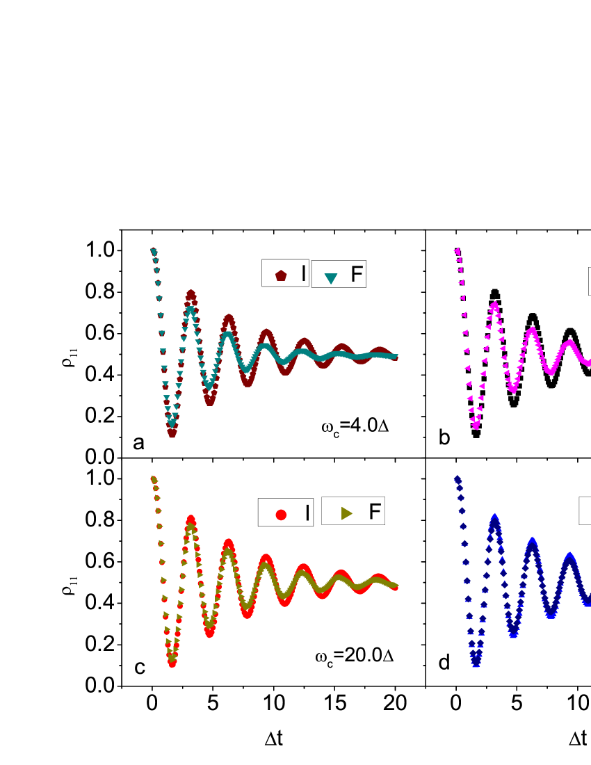
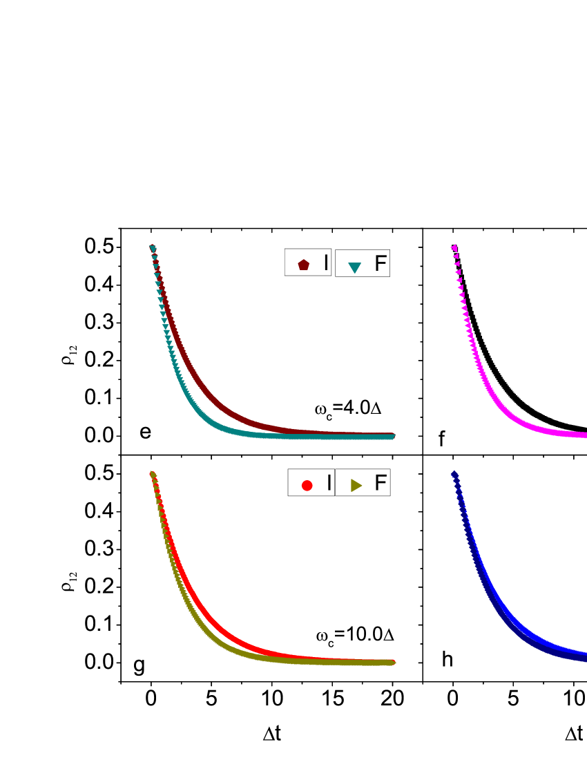
Figure 3: (Color online) The reduced dynamics of qubit in model B governed by $J_{B}^{I}\left(\omega\right)$ vs by $J_{B}^{F}\left(\omega\right)$ in different values of $\omega_{c}$. Here, $\lambda=1,\kappa_{1}=1,\eta^{\prime}=0.0035,$ and $\Gamma=52\Delta$, and the values of other parameters are the same as in Fig. 2.

If the quantum system of interest is a qubit the model B can be reduced to a spin-boson model as Eq.(15) with ESDF $J_{B}\left(\omega\right)$. By using the ITM algorithm we can also investigate the reduced dynamics of the qubit. The evolutions of the diagonal and off-diagonal elements of the reduced density matrix of the qubit governed by $J_{B}^{I}\left(\omega\right)$ and $J_{B}^{F}\left(\omega\right)$ are plotted in Fig.3 for the cases of $\omega_{c}=3.0\Delta,5.0\Delta,10.0\Delta,$ and $25.0\Delta$. Here, we set $\Omega_{0}=52.0\Delta$, and $\eta^{\prime}=0.0035$, and other parameters are the same as Fig.2. It is contrary to the case of model A, here the qubit has longer decoherence and relaxation times governed by the $J_{B}^{I}(\omega)$ than by $J_{B}^{F}(\omega)$.

As the cut-off frequency of the bath is not very large, the $J_{A}^{I}\left(\omega\right)$ results in shorter decoherence and relaxation times for the qubit in the models A than the $J_{A}^{F}\left(\omega\right)$ does. However, in model B, to compare to the $J_{B}^{F}\left(\omega\right)$, the $J_{B}^{I}\left(\omega\right)$ causes longer decoherence and relaxation times of the qubit, as the cut-off frequency of the bath is not very large. When the cut-off frequency of the bath increases to 5 times (for the model A) and 25 times (for the model B) of the characteristic frequency of the qubit, the $J_{A/B}^{F}\left(\omega\right)$ and the $J_{A/B}^{I}\left(\omega\right)$ will lead to almost the same reduced dynamics of the qubit for the respective models.

II.2 Two developed models (models C and D)

In this section we investigate the other two models C and D. These two models are developed from above two basic models A and B.

Model C: The Hamiltonian of the model C reads

$$H_{C} =\frac{p_{q}^{2}}{2\mu}+U\left(q\right)+\frac{P^{2}}{2M}+\frac{1}{2}M\Omega_{0}^{2}\left(X+\lambda q\right)^{2}$$

$$+{\textstyle\sum_{i}}\frac{p_{i}^{2}}{2m_{i}}+\frac{1}{2}m_{i}\omega_{i}^{2}\left(x_{i}+\frac{\kappa_{1}c_{i}X}{m_{i}\omega_{i}^{2}}\right)^{2}$$

$$+{\textstyle\sum_{j}}\frac{p_{j}^{2}}{2m_{j}}+\frac{1}{2}m_{j}\omega_{j}^{2}\left(x_{j}+\frac{\kappa_{2}c_{j}q}{m_{j}\omega_{j}^{2}}\right)^{2}.$$ (20)

Here, the quantum system of interest interacts with the IHO and both of them are coupled to their independent baths. The bath ($B_{1}$) coupled to the IHO and the bath ($B_{2}$) coupled to the quantum system of interest are considered to be constructed with two sets of harmonic oscillators and those mass, momentums, coordinates, and coupling coefficients are denoted by $\{m_{\alpha},$ $p_{\alpha},$ $x_{\alpha},$ $c_{\alpha}\}$ ($\alpha=i$ for $B_{1}$, and $\alpha=j$ for $B_{2}$). As $\kappa_{1}$, the $\kappa_{2}$ is also a controlling parameter for discussion. Similar to above subsection we can obtain an ESDF for the model as

$$J_{C}^{I}\left(\omega\right) =\eta\omega\kappa_{2}^{2}e^{-\omega/\omega_{c}}+\frac{\lambda^{2}\Omega_{0}^{4}\kappa_{1}^{2}\omega\eta}{\left(\omega^{2}-\Omega_{0}^{2}\right)^{2}e^{\omega/\omega_{c}}+\kappa_{1}^{2}\Gamma^{2}\omega^{2}e^{-\omega/\omega_{c}}},$$ (21)

when the cut-off frequency of the bath is infinite. Setting the cut-off frequency of the bath be finite, we have the ESDF for the model as

$$J_{C}^{F}\left(\omega\right) =\eta\omega\kappa_{2}^{2}\Theta\left(\omega\right)+\frac{\Omega_{0}^{4}\lambda^{2}\kappa_{1}^{2}\omega\eta\Theta\left(\omega\right)}{\Xi\left(\omega\right)^{2}+\kappa_{1}^{2}\omega^{2}\Gamma^{2}\Theta\left(\omega\right)^{2}}.$$ (22)

If both $\lambda$ and $\kappa_{1}$ are equal to zero, namely the quantum system of interest have not any interaction to other systems except for being directly coupled to a bath (where the bath is $B_{2}$) the model C will reduce to the model A, and from Eqs.(21) and (22), we can obtain

$$J_{C}^{I/F}\left(\omega\right)\xrightarrow{\lambda=\kappa_{1}=0}J_{A}^{I/F}\left(\omega\right).$$ (23)

When $\kappa_{2}=0$, the model C reduces to the model B which describes a quantum system of interest interacting with its environment through an IHO, and from Eqs.(21) and (22), we have

$$J_{C}^{I/F}\left(\omega\right)\xrightarrow{\kappa_{2}=0}J_{B}^{I/F}\left(\omega\right).$$ (24)

Model D: Model C describes that the quantum system of interest interacts with an IHO and both of them are coupled to two independent baths. However, when the quantum system is very closed to the IHO, they may embed in one common bath, then the Hamiltonian of the total system becomes

$$H_{D} =\frac{p_{q}^{2}}{2\mu}+U\left(q\right)+\frac{P^{2}}{2M}+\frac{1}{2}M\Omega_{0}^{2}\left(X+\lambda q\right)^{2}$$

$$+{\textstyle\sum_{i}}\frac{p_{i}^{2}}{2m_{i}}+\frac{1}{2}m_{i}\omega_{i}^{2}\left[x_{i}+\frac{c_{i}}{m_{i}\omega_{i}^{2}}\left(\kappa_{1}X+\kappa_{2}q\right)\right]^{2}.$$ (25)

Similarly, we can obtain an ESDF from infinite cut-off frequency as

$$J_{D}^{I}\left(\omega\right) =\lambda M\Omega_{0}^{2}\operatorname{Im}\Phi+\omega\eta\left[\kappa_{1}\kappa_{2}\operatorname{Re}\Phi+\kappa_{2}^{2}\right]e^{-\omega/\omega_{c}}.$$ (26)

Setting the cut-off frequency of the bath be finite, we have

$$J_{D}^{F}\left(\omega\right) =\lambda M\Omega_{0}^{2}\operatorname{Im}\Psi+\omega\eta\kappa_{1}\kappa_{2}\operatorname{Re}W\left(\omega\right)\operatorname{Im}\Psi$$

$$+\omega\eta\left[\kappa_{1}\kappa_{2}\operatorname{Re}\Psi+\kappa_{2}^{2}\right]\Theta\left(\omega\right),$$ (27)

where

$$\Phi =\frac{\Omega_{0}^{2}\lambda+i\Gamma\kappa_{2}\omega e^{-\omega/\omega_{c}}}{\left(\omega^{2}-\Omega_{0}^{2}\right)+i\kappa_{1}\omega\Gamma e^{-\omega/\omega_{c}}},$$ (28)

$$\Psi =\frac{\Omega_{0}^{2}\lambda+\Gamma\kappa_{2}\omega\operatorname{Re}W\left(\omega\right)+i\Gamma\kappa_{2}\omega\Theta\left(\omega\right)}{-\Xi\left(\omega\right)+i\kappa_{1}\omega\Gamma\Theta\left(\omega\right)}.$$ (29)

If we set $\kappa_{1}=0,$ $\lambda=0,$ and $\kappa_{2}=1,$ the model D will reduce to the model A and from Eqs.(26) and (27), we have

$$J_{D}^{I/F}\left(\omega\right)\xrightarrow{\lambda=\kappa_{1}=0,\kappa_{2}=1}J_{A}^{I/F}\left(\omega\right).$$ (30)

Setting $\kappa_{2}=0,$ the model D will reduce to the model B and from Eqs.(26) and (27), we can obtain

$$J_{D}^{I/F}\left(\omega\right)\xrightarrow{\kappa_{2}=0}J_{B}^{I/F}\left(\omega\right).$$ (31)

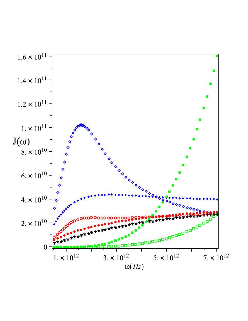
Figure 4: Effective spectral density functions, $J_{x}^{F}\left(\omega\right)$ in different models $x=A$ (black asterisk), $x=B$ (blue diamond), $x=C$ (red circle), and $x=D$ (green box), and $J_{x}^{I}\left(\omega\right)$ in different models $x=A$ (black cross), $x=B$ (blue solid diamond), $x=C$ (red solid circle), and $x=D$ (green solid box). Here, we set $\eta=0.02,\lambda=1,\kappa_{1}=\kappa_{2}=1,\Gamma=52\Delta,\Omega_{0}=10\Delta,\omega_{c}=11\Delta,\omega_{0}=10\Delta$

By using the ESDFs $J_{C}^{I/F}\left(\omega\right)$ and $J_{D}^{I/F}\left(\omega\right)$ we can compare the reduced dynamics of the qubit in models C and D, as we have done in last subsection. We can plot above different spectral density functions as Fig.4. Here, we are more interested in the question: in which model (C or D) the qubit has longer decoherence and relaxation times when the values of all of the parameters in the models are the same? Using the spectral density functions $J_{C}^{I/F}\left(\omega\right)$ of the model C, and $J_{D}^{I/F}\left(\omega\right)$ of the model D, we solve the reduced dynamics of the qubit in the two models. The evolutions of the elements of the reduced density matrix of the qubit are plotted in Fig.5. Here, we set $\kappa_{1}=\kappa_{2}=\lambda=1$, $\Omega_{0}=10\Delta$, and $\omega_{c}=7\Delta$. Other parameters are set with the same values as in Fig.2. It is shown that the qubit in the model D has longer decoherence and relaxation times than it has in the model C at the same finite cut-off frequency of the baths.

III Discussions and Conclusions

The spectral density function is in fact a bridge to connect the microcosmic and macroscopical physical quantities in dissipative quantum theory. At low temperature, the excitations of the bath modes with high frequencies are suppressed. So the spectral density function derived from infinite cut-off frequency of the bath will be out-of-true. In this paper we investigate the ESDFs $J_{x}^{I/F}\left(\omega\right)$ for models ($x=$A, B, C, D) at infinite and finite cut-off frequencies of baths from the microcosmic dynamical models by using the method initiated by Leggett et. al. As the cut-off frequency of the bath is comparable to the characteristic frequency of the quantum system of interest, the non-Markovian effects may also be important. In this case, it is improper to use any Markovian approximations to investigate the the reduced dynamics of quantum system. So we used a numerically exact ITM algorithm based on the QUAPI scheme solving the reduced dynamics of qubits.

In order to clearly compare the difference of the dynamics of quantum systems resulting from different ESDFs $J_{x}^{I}\left(\omega\right)$ and $J_{x}^{F}\left(\omega\right)$, we used the effective coupling constants calculating the dynamics of the qubit in each models and fixed other parameters such as the tempurature is set $300$k. It is shown that a qubit (the quantum system of interest) in these models has different dynamics when they are governed by the spectral density functions $J_{x}^{I}\left(\omega\right)$ and $J_{x}^{F}\left(\omega\right)$ as the cut-off frequencies are not too large. The difference increase with the decrease of the cut-off frequency. When the cut-off frequencies of the baths are larger about 5 times (for the models based on model A) and 25 times (for the models based on model B) than the characteristic frequency of the qubit, the two kinds of spectral density functions result in almost the same reduced dynamics. In addition, we obtain that a qubit will have longer relaxation and decoherence times when it is coupled to an IHO and both of them are coupled to a common bath rather than to their respective baths.

Acknowledgement 1

This project was sponsored by National Natural Science Foundation of China (Grant No. 10675066), Natural Science Foundation of Ningbo City (Grant No.2008A610098) and K C Wong Magna Foundation in Ningbo University.

IV Appendix

In the Appendix we give a proof of Eq.(11), namely prove equation $R\left(\omega\right)=-\frac{\pi i}{\omega}e^{-\omega/\omega c}-\frac{\pi}{\omega}W\left(\omega\right).$ Setting

$$z=x+iy,\text{ }f\left(z\right)=\frac{\exp(-z/\omega_{c})}{\left(z^{2}-\omega^{2}\right)},$$ (32)

and from Fig.5 we see that there is not any singular point in the loop of $(L+\overline{M_{2}0}+\overline{0M_{1}}+C)$. So by using the Cauchy’s theorem we have

$$\underset{G_{I}}{\underbrace{\int_{L}f(z)dz}}+\underset{G_{II}}{\underbrace{\int_{R}^{0}f(iy)d\left(iy\right)}}+\underset{G_{III}=R\left(\omega\right)}{\underbrace{\int_{0}^{R}f(x)d\left(x\right)}}+\underset{G_{IV}}{\underbrace{\int_{C}f(z)dz}}=0.$$ (33)

For curve $L$, because

$$\lambda_{1}=\lim_{R\rightarrow\infty}zf(z)=\lim_{R\rightarrow\infty}\frac{\exp(-z/\omega_{c})}{\left(z-\omega^{2}/z\right)}=0,$$ (34)

we have

$$G_{I}=\int_{L}f(z)dz=i\left(\theta_{2}-\theta_{1}\right)\lambda_{1}=0.$$ (35)

For curve $C$, we replace pramaters $z$ and $\omega$ with $r$ and $\varphi$ and setting $z-\omega=re^{i\varphi}.$ Because $\varphi_{2}=\pi,$ $\varphi_{1}=0,$ and

$$\lambda_{2}=\lim_{r\rightarrow 0}zf(z)=\frac{\exp(-\omega/\omega_{c})}{2\omega},$$ (36)

we have

$$G_{IV}=\int_{c}f(z)dz=i\left(\varphi_{2}-\varphi_{1}\right)\lambda_{2}=\frac{i\pi\exp(-\omega/\omega_{c})}{2\omega}.$$ (37)

For linear $\overline{M_{2}0}$, the integral becomes

$$G_{II}=\int_{R}^{0}f(iy)d\left(iy\right)=-\frac{i}{\omega}\int_{R}^{0}\frac{\exp(-i\frac{y}{\omega}\cdot\frac{\omega}{\omega_{c}})}{\left(\frac{y}{\omega}\right)^{2}+1}d\left(\frac{y}{\omega}\right).$$ (38)

Setting $\frac{y}{\omega}=x,\frac{\omega}{\omega_{c}}=m,$ we have

$$G_{II} =-\frac{i}{\omega}\int_{R}^{0}\frac{\exp(-ixm)}{x^{2}+1}d\left(x\right)$$

$$=-\frac{i}{\omega}\int_{R}^{0}\frac{\cos mx}{x^{2}+1}d\left(x\right)-\frac{1}{\omega}\int_{R}^{0}\frac{\sin mx}{x^{2}+1}d\left(x\right).$$ (39)

Here,

$$\int_{R}^{0}\frac{\cos mx}{x^{2}+1}d\left(x\right)$$

$$=-\int_{0}^{R}\frac{\cos mx}{x^{2}+1}d\left(x\right)=-\frac{\pi}{2}\exp(-\omega/\omega_{c}),$$ (40)

$$\int_{R}^{0}\frac{\sin mx}{x^{2}+1}d\left(x\right)$$

$$=-Shi\left(m\right)\cosh\left(m\right)+\operatorname{Ci}\left(-im\right)\sinh\left(m\right)+\frac{\pi i}{2}\sinh\left(m\right)$$

$$\equiv\pi W\left(\omega\right).$$ (41)

with

$$Shi(m) =\int_{0}^{m}\frac{\sinh(t)}{t}dt,$$ (42)

$$\operatorname{Ci}(m) =\int_{0}^{\infty}e^{-t}t^{(m-1)}dt+\ln(m)+\int_{0}^{m}\frac{\cos(t)-1}{t}dt.$$ (43)

So we have

$$G_{II}=\frac{\pi i}{2\omega}e^{-\omega/\omega c}+\frac{\pi}{\omega}W\left(\omega\right).$$ (44)

From Eqs.(33), (35), (37), and (44) we have the integral in linear $\overline{0M_{1}}$ as

$$G_{III} =\int_{0}^{R}f(x)d\left(x\right)$$

$$=-G_{I}-G_{II}-G_{IV}$$

$$=-\frac{\pi i}{2\omega}e^{-\omega/\omega c}-\frac{\pi i}{2\omega}e^{-\omega/\omega c}-\frac{\pi}{2\omega}W\left(\omega\right)$$

$$=-\frac{\pi i}{\omega}e^{-\omega/\omega c}-\frac{\pi}{\omega}W\left(\omega\right)$$

$$=R\left(\omega\right).$$ (45)

Figure 1: (Color online) The values of $\operatorname{Im}[W\left(\omega\right)]$ when choosing the cut-off frequency $\omega_{c}$ different values. It is shown that the absolute values of $\operatorname{Im}[W\left(\omega\right)]$ decreases with the increase of the cut-off frequency of the bath $\omega_{c}$

.

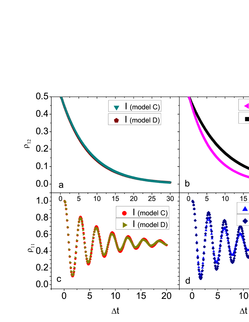
Figure 5: (Color online) The reduced dynamics of the qubit in model C versus in model D governed by the ESDFs $J_{C}^{I/F}\left(\omega\right)$ and $J_{D}^{I/F}\left(\omega\right)$. Top two figures a and b plot the evolutions of the off-diagonal $\rho_{12}(t)$. Bottom two figures plot the evolutions of the diagonal elements $\rho_{11}(t)$. Here, $\kappa_{1}=\kappa_{2}=\lambda=1,\eta^{\prime}=0.0035$, and $\omega_{c}=7\Delta,\Omega_{0}=10\Delta,$ and the values of the other parameters are the same as in Fig 2.

Figure 6: Integral scheme of Eq.33

References

- (1) A. O. Caldeira, and A. J. Leggett, Ann. Phys. 149, 374 (1983).
- (2) U. Weiss, Quantum Dissipative Systems, 2nd ed., (World Scientific Publishing, Singapore, 1999).
- (3) A. J. Leggett, S. Chakravarty, A. T. Dorsey, M. P. A. Fisher, A. Garg, and W. Zwerger, Rev. Mod. Phys. 59, 1 (1987).
- (4) A. J. Leggett, Phys. Rev. B 30, 1208 (1984).
- (5) A. Garg, J. N. Onuchic, and V. Ambegaokar, J. Chem. Phys. 83, 4491 (1985).
- (6) H. Grabert, P. Schramm, and G. -L. Ingold, Phys. Rep. 168, 115 (1988).
- (7) X.-T. Liang, Chem. Phys. Lett. 449, 296 (2007); X. -T. Liang, Chem. Phys. 352, 106 (2008).
- (8) M. W. Y. Tu, and W.-M. Zhang, Phys. Rev. B 78, 235311 (2008).
- (9) M.-T. Lee, and W. -M. Zhang, J. Chem. Phys. 129, 224106 (2008).
- (10) J. -Q. You, Y. -X. Liu, C. -P. Sun, and F. Nori, Phys. Rev. B 75, 104516 (2007).
- (11) F. Nesi, E. Paladino, M. Thorwart, M Grifoni, Phys. Rev. B 76, 155323 (2007).
- (12) E. Ferraro, M. Scala, R. Migliore, and A. Napoli, Phys. Rev A 80, 042112 (2009).
- (13) C. Gan, and H. Zheng, Phys. Rev. A 80, 041106 (2009).
- (14) A. Bassi, and L. Ferialdi, Phys. Rev. Lett. 103, 050403 (2009).
- (15) R. L. S. Farias, R. O. Ramos,and L. A. da Silva, Phys. Rev. A 80, 031143 (2009).
- (16) D. Abramavicius, B. Palmieri, D.V. Voronine, F. Šanda, S Mukamel, Chem. Rev. 109, 2350 (2009).
- (17) A. Ishizaki, and Y. Tanimura, Chem. Phys. 347, 185 (2008).
- (18) H. Lee, Y.-C. Cheng, and G. R. Fleming, Science 316, 1462 (2007).
- (19) G. S. Engel, T. R. Calhoun, E. L. Read, T. -K. Ahn, T. Mančal, Y. -C. Cheng, R. E. Blankenship, and G. R. Fleming, Nature 446, 782 (2007).
- (20) S. T. Smith, and R. Onofrio, Eur. Phys. J. B 61, 271 (2008).
- (21) Q. Wei, S. T. Smith, and R. Onofrio, Phys. Rev. E 79, 031128 (2009).
- (22) Tanimura, and Wolynes, J. Chem. Phys. 96, 8485 (1992).
- (23) M. Schroeder, M. Schreiber, and U. Kleinekathoefer, J. Chem. Phys. 126, 114102 (2007).
- (24) Q. Shi, L. Chen, G. Nan, R. Xu, and Y. Yan, J. Chem. Phys. 130, 164518 (2009).
- (25) B. Palmieri, D. Abramavicius, and S. Mukamel, J. Chem. Phys. 130, 204512 (2009).
- (26) Y. Tanimura, J. Phys. Soc. Jpn. 75, 0082001 (2006).
- (27) M. Tanaka, and Y. Tamimura, J. Phys. Soc. Jpn. 78, 073802 (2009).
- (28) N. Makri, D.E. Makarov, J. Chem. Phys. 102, 4600 (1995).
- (29) D.E. Makarov, N. Makri, Chem. Phys. Lett. 221, 482 (1994).
- (30) N. Makri, E. Sim, D. E. Makarov, and M. Topaler, Proc. Natl. Acad. Sci. USA 93, 3926 (1996).
- (31) M. Thorwart, P. Reimann, P. Hänggi, Phys. Rev. E 62, 5808 (2000).
- (32) X.-T. Liang, Phys. Rev. B 72, 245328 (2005).
.