Derivative expansion for the boundary interaction terms in the Casimir effect: generalized $\delta$-potentials

Abstract

We calculate the Casimir energy for scalar fields in interaction with finite-width mirrors, described by nonlocal interaction terms. These terms, which include quantum effects due to the matter fields inside the mirrors, are approximated by means of a local expansion procedure. As a result of this expansion, an effective theory for the vacuum field emerges, which can be written in terms of generalized $\delta$-potentials. We compute explicitly the Casimir energy for these potentials and show that, for some particular cases, it is possible to reinterpret them as imposing imperfect Dirichlet boundary conditions.

I Introduction

Casimir forces are a striking manifestation of the zero-point energy of the electromagnetic field in the presence of ‘mirrors’ endowed with quite general electromagnetic properties reviews . In many calculations of the Casimir energies and forces, the presence of the mirrors is modeled by appropriate boundary conditions on the interfaces of the different media, that include macroscopic parameters such as their electric permitivity, magnetic permeability, conductivity, etc. A first-principles calculation of the Casimir energy should consider the microscopic degrees of freedom associated to the mirrors. This could shed light on some interesting open questions, the role of dissipation on the Casimir energy being, perhaps, the most important among them.

In a previous paper Fosco:2008td , we considered the Casimir effect for scalar and gauge fields interacting with dynamical matter on thin mirrors (see also Ref.graphene for a concrete model realization). More recently, one of us considered the generalization to the case of finite-width mirrors Fosco:2009cw . The interaction between the vacuum scalar field and the mirrors’ degrees of freedom gives rise, in general, to a nonlocal effective action in terms of which the Casimir energy may be calculated extra . Moreover, under certain circumstances, it is possible to find a formal expression for the Casimir energy in terms of the parameters that define the nonlocal kernel Fosco:2009cw . In this paper, we will present an application of the previously developed formalism for the Casimir effect with nonlocal boundary interaction terms, to situations where those nonlocal terms may be expanded in a series of local ones. In other words, we will perform a derivative expansion of the nonlocal effective action. One should expect on physical grounds that, in many relevant cases, such a local description of the mirrors must be reliable. We show here how one can indeed find such an expansion, and then we shall apply it to derive approximate expressions for the Casimir energy.

The structure of this paper is the following. In Section II, we derive the derivative expansion for the nonlocal effective action, which will be written in terms of a set of generalized $\delta$-potentials, i.e. terms proportional to Dirac’s $\delta$-function and its derivatives. We will illustrate, in concrete examples, how the coupling between the vacuum field and the microscopic degrees of freedom, together with the boundary conditions that confine the microscopic degrees of freedom inside the mirrors, do determine the different coefficients in the derivative expansion. In Section III we compute the Casimir energy for the resulting generalized $\delta$-potentials. Section IV contains our final remarks.

II Derivative expansion of the nonlocal effective action

Let us consider a real scalar field $\varphi$ in the presence of two flat mirrors of width $\epsilon$ centered at $x_{d}=0,\,a$. This scalar field interacts with the microscopic degrees of freedom inside the mirrors, which in the specific examples below will be described by a second scalar field $\chi$. After integrating the microscopic degrees of freedom of the mirrors, the effective action for the scalar field $\varphi$ will be of the form

$$S(\varphi)=\frac{1}{2}\int d^{d}x_{\parallel}dx_{d}\left(\partial\varphi\right)^{2}+S_{I}^{(0)}(\varphi)+S_{I}^{(a)}(\varphi),$$ (1)

where $S_{I}^{(0)}$ and $S_{I}^{(a)}$ are concentrated on the positions of each mirror. On general grounds we expect these interaction terms to be nonlocal, i.e.,

$$S_{I}^{(0)}(\varphi)\;=\;\frac{1}{2}\,\int_{-\infty}^{+\infty}dx_{d}\int_{-\infty}^{+\infty}dx^{\prime}_{d}\int\frac{d^{d}k_{\parallel}}{(2\pi)^{d}}\;{\widetilde{\varphi}}^{*}(k_{\parallel},x_{d}){\widetilde{V}}_{\epsilon}(k_{\parallel};x_{d},x^{\prime}_{d}){\widetilde{\varphi}}(k_{\parallel},x^{\prime}_{d})\;,$$ (2)

and a similar expression for $S_{I}^{(a)}$. Here $x_{\parallel}$ denotes the time ($x_{0}$) as well as the $d-1$ spatial coordinates parallel to the mirror (which we shall denote by $\mathbf{x_{\parallel}}$). We have assumed translational invariance in the coordinates $x_{\parallel}$, and therefore it is useful to write the effective action in terms of the Fourier transform of the field in these coordinates, $\widetilde{\varphi}$, with the obvious notation $k_{\parallel}$ for the argument of this function.

The nonlocal kernel ${\widetilde{V}}_{\epsilon}$ may be expanded as follows Fosco:2009cw

$${\widetilde{V}}_{\epsilon}(k_{\parallel};x_{d},x^{\prime}_{d})\;=\;\sum_{m,n}\psi_{m}^{(\epsilon)}(x_{d})\,C_{mn}(k_{\parallel},\epsilon)\psi_{n}^{(\epsilon)*}(x^{\prime}_{d})\;,$$ (3)

and the functions $\psi_{n}^{(\epsilon)}(x_{d})$ depend essentially on the nature of the boundary conditions for the microscopic fields (i.e., those living inside the mirrors) while the coefficients, $C_{mn}(k_{\parallel},\epsilon)$, are obtained by taking into account the (kinematic and dynamical) properties of those fields. Eq. (2) results from the assumption that, after integrating the microscopic fields, the most relevant term in the effective action is quadratic in the scalar field; in other words, we are assuming, as usual, that the media can be described by linear response theory. The particular case in which the interaction between the thick mirrors and the vacuum field is approximated by a local effective action (i.e. ${\widetilde{V}}_{\epsilon}(k_{\parallel};x_{d},x^{\prime}_{d})=f(k_{\parallel},x_{d})\delta(x_{d}-x^{\prime}_{d})$) has been considered in Ref.prd08 .

As we will see, the nonlocal effects can be evaluated perturbatively by expanding the kernel ${\widetilde{V}}_{\epsilon}$ in powers of the $\delta$-function and its derivatives:

$${\widetilde{V}}_{\epsilon}(k_{\parallel};x_{d},x^{\prime}_{d})\;=\;\tilde{\mu}_{0}(k_{\parallel})\delta(x_{d})\delta(x^{\prime}_{d})+\tilde{\mu}_{1}(k_{\parallel})\left(\delta(x_{d})\delta^{\prime}(x^{\prime}_{d})+\delta^{\prime}(x_{d})\delta(x^{\prime}_{d})\right)+\tilde{\mu}_{2}(k_{\parallel})\delta^{\prime}(x_{d})\delta^{\prime}(x^{\prime}_{d})+...$$ (4)

where $\tilde{\mu}_{i}(k_{\parallel})$ depend on the microscopic fields and their interaction with the vacuum field.

We start our derivation of the expansion with the study of a simple example, namely, the case in which the microscopic field $\chi$ is also a real scalar, endowed with a quadratic action, and linearly coupled to $\varphi$. As already mentioned, we denote by $\epsilon$ the width of the mirror, which fills the region $-\epsilon/2\leq x_{d}\leq\epsilon/2$. Then, as shown in Fosco:2009cw , the coefficients $C_{mn}(k_{\parallel},\epsilon)$ adopt the diagonal form:

$$C_{mn}(k_{\parallel},\epsilon)\;=\;\frac{g^{2}}{\xi_{n}^{2}+k_{\parallel}^{2}+m^{2}}\,\delta_{mn}\;,$$ (5)

where $m$ is the mass of the microscopic field, $\xi_{n}^{2}$ ($\xi_{n}\in{\mathbb{R}}$) denote the eigenvalues of $(-\partial_{d}^{2})$ corresponding to the eigenvectors $\psi_{n}^{(\epsilon)}(x_{d})$, and $g$ is the coupling constant between $\varphi$ and $\chi$.

The precise form of those eigenvalues and eigenvectors depends of course on the boundary conditions for the microscopic field. Indeed, for the case of Dirichlet boundary conditions, we have the eigenfunctions:

$$\psi_{n}^{(\epsilon)}(x_{d})\;=\;\sqrt{\frac{2}{\epsilon}}\,\times\,\left\{\begin{array}[]{lcll}\sin(\frac{n\pi x_{d}}{\epsilon})&{\rm if}&\;n=2k,&(k=1,2,\ldots)\\ \cos(\frac{n\pi x_{d}}{\epsilon})&{\rm if}&\;n=2k+1,&(k=0,1,\ldots)\;,\end{array}\right.$$ (6)

while in the Neumann case, we have instead

$$\psi_{n}^{(\epsilon)}(x_{d})\;=\;\frac{1}{\sqrt{\epsilon}}\times\,\left\{\begin{array}[]{ccll}1&{\rm if}&n=0,&\\ \sqrt{2}\,\sin(\frac{n\pi x_{d}}{\epsilon})&{\rm if}&\;n=2k+1,&(k=0,1,\ldots)\\ \sqrt{2}\,\cos(\frac{n\pi x_{d}}{\epsilon})&{\rm if}&\;n=2k,&(k=1,2,\ldots)\;.\end{array}\right.$$ (7)

The eigenvalues are then, in both cases, given by the expression: $\xi_{n}^{2}=\big{(}\frac{\pi n}{\epsilon}\big{)}^{2}$, where $n=1,2,\ldots$ in the Dirichlet case, while for Neumann boundary conditions: $n=0,1,2,\ldots$

The essential difference is thus the existence or not of a zero mode, which is present only in the Neumann case. One should expect this difference to manifest itself when one tries to perform a local approximation for the nonlocal interaction term, under the assumption that $\epsilon\to 0$. Indeed, note that, in such a case, the zero mode is multiplied by the $\epsilon$-independent coefficient $C_{00}$, while all the other $C_{mn}$ coefficients are relatively suppressed in such a limit. To make this statement more precise, let us perform an expansion of the interaction term, assuming that $\epsilon$ is small (this shall be made more clear below, after introducing the other length scale to compare it with).

We shall assume, in what follows, Neumann boundary conditions for the microscopic field. Writing $S_{I}^{(0)}$ more explicitly:

$$S_{I}^{(0)}(\varphi)\;=\;\frac{1}{2}\,g^{2}\,\int\frac{d^{d}k_{\parallel}}{(2\pi)^{d}}\;\sum_{m,n=0}\,\langle{\widetilde{\varphi}}|\psi_{n}^{(\epsilon)}\rangle\,\frac{1}{\xi_{n}^{2}+k_{\parallel}^{2}+m^{2}}\,\langle\psi_{n}^{(\epsilon)}|{\widetilde{\varphi}}\rangle\;,$$ (8)

where we used the notation $\langle f|g\rangle\equiv\int_{-\frac{\epsilon}{2}}^{+\frac{\epsilon}{2}}dx_{d}\,f^{*}(x_{d})\,g(x_{d})$.

Let us first consider the leading term in a small-$\epsilon$ expansion, obtained by keeping only the zero mode contribution. This may be written as follows:

$$S_{I}^{(0)}(\varphi)\,\approx\,\frac{1}{2}\,g^{2}\epsilon\,\int\frac{d^{d}k_{\parallel}}{(2\pi)^{d}}\,\frac{1}{k_{\parallel}^{2}+m^{2}}\;\int_{-\infty}^{+\infty}dx_{d}\,\delta_{\epsilon}(x_{d}){\widetilde{\varphi}}^{*}(k_{\parallel},x_{d})\int_{-\infty}^{+\infty}dx^{\prime}_{d}\,\delta_{\epsilon}(x^{\prime}_{d}){\widetilde{\varphi}}(k_{\parallel},x^{\prime}_{d})$$ (9)

where we introduced $\delta_{\epsilon}(x_{d})\equiv\theta\big{(}\frac{\epsilon}{2}-|x_{d}|\big{)}/\epsilon$, which works as an approximant of Dirac’s $\delta$-function. Then we see that this leading term may be regarded as a local $\delta$-function term, with a momentum-dependent strength, and affected by a coefficient $g^{2}\epsilon$. It is convenient to introduce the product $g^{2}\epsilon\equiv\lambda$, since that is the constant that determines the strength of the boundary interaction term:

$$S_{I}^{(0)}(\varphi)\,\to\,\frac{1}{2}\,\lambda\,\int\frac{d^{d}k_{\parallel}}{(2\pi)^{d}}\int_{-\infty}^{+\infty}dx_{d}\,\frac{1}{k_{\parallel}^{2}+m^{2}}\;\delta(x_{d})\,{\widetilde{\varphi}}^{*}(k_{\parallel},x_{d}){\widetilde{\varphi}}(k_{\parallel},x_{d})\;.$$ (10)

The following terms in the expansion are obtained by expanding the overlaps $\langle\psi_{n}^{(\epsilon)}|\widetilde{\varphi}\rangle$ for small $\epsilon$, by using a Taylor expansion for the vacuum field. Up to the second order in derivatives, we find:

$$\langle\psi_{n}^{(\epsilon)}|\widetilde{\varphi}\rangle\;=\;\sqrt{\epsilon}\times\,\left\{\begin{array}[]{cll}{\widetilde{\varphi}}(k_{\parallel},0)&{\rm if}\;n=0&\\ \sqrt{2}\,\frac{\epsilon}{\pi^{2}}\,\frac{2}{(2k+1)^{2}}\,(-1)^{k}\;\big{[}\partial_{d}{\widetilde{\varphi}}(k_{\parallel},x_{d})\big{]}_{x_{d}=0}&{\rm if}\;n=2k+1&(k=0,1,\ldots)\\ \sqrt{2}\big{(}\frac{\epsilon}{\pi}\big{)}^{2}\,\frac{1}{(2k)^{2}}\,(-1)^{k}\;\big{[}\partial^{2}_{d}{\widetilde{\varphi}}(k_{\parallel},x_{d})\big{]}_{x_{d}=0}&{\rm if}\;n=2k&(k=1,2,\ldots)\end{array}\right.\;.$$ (11)

We see that the assumption that one could use to justify the expansion a posteriori is that the field inside the mirror should not change appreciably inside the mirror, more precisely, the length scale of the spatial variation should be much larger than $\epsilon$. This means that higher powers of $\epsilon$ will be attached to higher derivatives of the field.

Equipped with the expansion (11), we obtain the corresponding expansion of $S_{I}^{(0)}$ up to the second order in derivatives:

$$S_{I}^{(0)}\;=\;S_{I,0}^{(0)}\,+\,S_{I,2}^{(0)}\,+\,\ldots$$ (12)

where $S_{I,0}^{(0)}$ coincides with Eq.(9), while:

$$S_{I,2}^{(0)}=\frac{1}{2}\,g^{2}\,8\,\epsilon\,(\frac{\epsilon}{\pi})^{2}\,\int\frac{d^{d}k_{\parallel}}{(2\pi)^{d}}\;\big{|}{\widetilde{\varphi}}^{\prime}(k_{\parallel},0)\big{|}^{2}\,\sum_{l=0}^{\infty}\frac{1}{(2l+1)^{2}\Big{[}(2l+1)^{2}(\frac{\pi}{\epsilon})^{2}+k_{\parallel}^{2}+m^{2}\Big{]}}\;.$$ (13)

Here the prime denotes derivative with respect to $x_{d}$. Performing the sum of the series, we obtain

$$S_{I,2}^{(0)}=\frac{1}{2}\,g^{2}\,8\,\epsilon^{3}\,\int\frac{d^{d}k_{\parallel}}{(2\pi)^{d}}\;\big{|}{\widetilde{\varphi}}^{\prime}(k_{\parallel},0)\big{|}^{2}\,\frac{1}{\big{[}\omega(k_{\parallel})\big{]}^{2}}\,\Big{\{}\frac{1}{8}-\frac{1}{4\epsilon\,\omega(k_{\parallel})}\,\tanh\big{[}\frac{\epsilon\,\omega(k_{\parallel})}{2}\big{]}\Big{\}}\;,$$ (14)

where $\omega(k_{\parallel})\equiv\sqrt{k_{\parallel}^{2}+m^{2}}$. We may again write this term in a similar fashion to (9):

$$S_{I,2}^{(0)}(\varphi)\,\approx\,\frac{1}{2}\,\lambda\,\int\frac{d^{d}k_{\parallel}}{(2\pi)^{d}}\,f(k_{\parallel},\epsilon)\,\frac{1}{\big{[}\omega(k_{\parallel})\big{]}^{2}}\;\int_{-\infty}^{+\infty}dx_{d}\,\delta^{\prime}(x_{d}){\widetilde{\varphi}}^{*}(k_{\parallel},x_{d})\int_{-\infty}^{+\infty}dx^{\prime}_{d}\,\delta^{\prime}(x^{\prime}_{d}){\widetilde{\varphi}}(k_{\parallel},x^{\prime}_{d})$$ (15)

with

$$f(k_{\parallel},\epsilon)\;=\;\epsilon^{2}\,\Big{\{}1-\frac{2}{\epsilon\,\omega(k_{\parallel})}\,\tanh\big{[}\frac{\epsilon\omega(k_{\parallel})}{2}\big{]}\Big{\}}\;.$$ (16)

We will now summarize the result for the expansion of the nonlocal term, presenting it in a way which shall be useful in the derivation of the Casimir energy. Thus, we encode the results as follows: the expansion for the interaction action (2) may be interpreted as an expansion for the nonlocal potential, so that:

$${\widetilde{V}}_{\epsilon}(k_{\parallel};x_{d},x^{\prime}_{d})\;=\;{\widetilde{V}}_{\epsilon,0}(k_{\parallel};x_{d},x^{\prime}_{d})\,+\,{\widetilde{V}}_{\epsilon,2}(k_{\parallel};x_{d},x^{\prime}_{d})\,+\,\ldots$$ (17)

where:

$${\widetilde{V}}_{\epsilon,0}(k_{\parallel};x_{d},x^{\prime}_{d}) = \tilde{\mu}_{0}(k_{\parallel},\epsilon)\,\delta(x_{d})\,\delta(x^{\prime}_{d})$$

$${\widetilde{V}}_{\epsilon,2}(k_{\parallel};x_{d},x^{\prime}_{d}) = \tilde{\mu}_{2}(k_{\parallel},\epsilon)\,\delta^{\prime}(x_{d})\,\delta^{\prime}(x^{\prime}_{d})$$ (18)

with $\tilde{\mu}_{0}(k_{\parallel},\epsilon)=\frac{\lambda}{[\omega(k_{\parallel})]^{2}}$ and $\tilde{\mu}_{2}(k_{\parallel},\epsilon)=\frac{\lambda f(k_{\parallel},\epsilon)}{[\omega(k_{\parallel})]^{2}}$.

It is worth noting that the derivative expansion of the effective action for the specific example considered so far does not include terms containing only one derivative of the scalar field (i.e. terms proportional to $\tilde{\mu}_{1}(k_{\parallel})$, see Eq.(4)). This is due to the fact that the eigenfunctions in Eqs.(6) and (7) have a definite parity in the interval $-\epsilon/2\leq x_{d}\leq\epsilon/2$. Therefore, we expect such terms to show up only if one considered ‘non-symmetric’ mirrors in which the boundary conditions that confine the microscopic fields are different on both interfaces $x_{d}=\pm\epsilon/2$, for example $\chi(-\epsilon/2)=0,\partial_{d}\chi(\epsilon/2)=0$.

Up to here, we considered a microscopic field $\chi$ linearly coupled to $\varphi$. The expansions presented in Eqs.(17) and (18) remain valid when the microscopic $\chi$-field is nonlinearly coupled to $\varphi$. To illustrate this fact, we will now consider a different case, i.e. we shall deal with a $g\chi^{2}\varphi$ coupling term for $d=3$. In terms of the eigenfunctions $\psi_{n}^{(\epsilon)}$, the second order term in the expansion of the action $S_{I}(\varphi)$ is given by:

$$S^{(0)}_{I}\approx g^{2}\int\frac{d^{3}k_{\parallel}}{(2\pi)^{3}}\left|\tilde{\varphi}(k_{\parallel},0)\right|^{2}\int\frac{d^{3}p_{\parallel}}{(2\pi)^{3}}\int_{-\infty}^{+\infty}dx_{d}\int_{-\infty}^{+\infty}dx_{d}^{\prime}\sum_{n,m}\frac{\psi_{n}^{(\epsilon)}(x_{d})\psi_{n}^{(\epsilon)}(x_{d}^{\prime})\psi_{m}^{(\epsilon)}(x_{d})\psi_{m}^{(\epsilon)}(x_{d}^{\prime})}{\left(\xi_{n}^{2}+m^{2}+p_{\parallel}^{2}\right)\left(\xi_{m}^{2}+m^{2}+(p_{\parallel}+k_{\parallel})^{2}\right)}\;.$$ (19)

The integrations over normal coordinates ($x_{d}$ and $x_{d}^{\prime}$) can be trivially performed by means of the orthogonality conditions of the eigenfunctions $\psi_{n}^{(\epsilon)}$, obtaining

$$S^{(0)}_{I}\approx g^{2}\int\frac{d^{3}k_{\parallel}}{(2\pi)^{3}}\left|\tilde{\varphi}(k_{\parallel},0)\right|^{2}\sum_{n}\int\frac{d^{3}p_{\parallel}}{(2\pi)^{3}}\frac{1}{\left(\xi_{n}^{2}+m^{2}+p_{\parallel}^{2}\right)\left(\xi_{n}^{2}+m^{2}+(p_{\parallel}+k_{\parallel})^{2}\right)}\;.$$ (20)

After integrating over $p_{\parallel}$, one sees that the interaction action becomes

$$S^{(0)}_{I}\approx\frac{g^{2}}{4\pi}\int\frac{d^{3}k_{\parallel}}{(2\pi)^{3}}\left|\tilde{\varphi}(k_{\parallel},0)\right|^{2}\sum_{n}\frac{1}{k_{\parallel}}\arctan{\left\{\frac{k_{\parallel}}{2\sqrt{\xi_{n}^{2}+m^{2}}}\right\}},$$ (21)

whence one can read the coefficient $\tilde{\mu}_{0}(k_{\parallel},\epsilon)$ in Eq.(18),

$$\tilde{\mu}_{0}(k_{\parallel},\epsilon)=\frac{g^{2}}{4\pi}\frac{1}{k_{\parallel}}\sum_{n}\arctan{\left\{\frac{\epsilon k_{\parallel}}{2\sqrt{n^{2}\pi^{2}+\epsilon^{2}m^{2}}}\right\}},$$ (22)

where we have used that $\xi_{n}^{2}=\left(\frac{n\pi}{\epsilon}\right)^{2}$.

The sum in last equation runs from $0$ for Neumann boundary conditions, and from $1$ for Dirichlet ones. Eq.(22) is divergent for large $n$, therefore we introduce a renormalization term, in order to obtain a finite coefficient. For a massless field with Dirichlet boundary conditions we obtain:

$$\tilde{\mu}_{0}(k_{\parallel},\epsilon)={\bar{\mu}}_{0}+\frac{g^{2}}{4\pi}\sum_{n\geq 1}\left[\frac{1}{k_{\parallel}}\arctan{\big{(}\frac{\epsilon k_{\parallel}}{2n\pi}\big{)}}-\frac{\epsilon}{2n\pi}\right],$$ (23)

where ${\bar{\mu}}_{0}$ is a renormalization constant. We note that, contrary to what happens for the case of a linear coupling, we obtain a contribution whose strength is independent of $\epsilon$.

In the case of Neumann boundary conditions:

$$\tilde{\mu}_{0}(k_{\parallel},\epsilon)={\bar{\mu}}_{0}+\frac{g^{2}}{4\pi}\frac{1}{k_{\parallel}}\arctan{\big{(}\frac{k_{\parallel}}{2m}\big{)}}+\frac{g^{2}}{4\pi}\sum_{n\geq 1}\left[\frac{1}{k_{\parallel}}\arctan{\big{(}\frac{\epsilon k_{\parallel}}{2\sqrt{n^{2}\pi^{2}+\epsilon^{2}m^{2}}}\big{)}}-\frac{\epsilon}{2n\pi}\right]\;,$$ (24)

which in the case of a massless microscopic field becomes:

$$\tilde{\mu}_{0}(k_{\parallel},\epsilon)={\bar{\mu}}_{0}\,+\,g^{2}\,\left\{\frac{1}{8\,k_{\parallel}}+\frac{1}{4\pi}\sum_{n\geq 1}\Big{[}\frac{1}{k_{\parallel}}\arctan{\big{(}\frac{\epsilon k_{\parallel}}{2n\pi}}\big{)}-\frac{\epsilon}{2n\pi}\Big{]}\right\}\;.$$ (25)

We note that the previous series can be summed, the exact result being

$$\tilde{\mu}_{0}(k_{\parallel},\epsilon)={\bar{\mu}}_{0}-\frac{g^{2}}{8\pi k_{\parallel}}\left\{\frac{\epsilon\gamma k_{\parallel}}{\pi}+2{\rm Arg}\Gamma(\frac{ik_{\parallel}\epsilon}{2\pi})\right\}.$$ (26)

The computation of $\tilde{\mu}_{2}$ can be performed along similar lines, although is much more cumbersome and we will not present the details here.

To summarize, in this Section we have shown that the nonlocal interaction between the mirror and the scalar field admits a derivative expansion of the kind given in Eq.(4), where the coefficients $\tilde{\mu}_{i}$ depend not only on $k_{\parallel}$ but also on the width $\epsilon$ of the mirror. It is possible to adjust the relation of the coupling constants and $\epsilon$ in such a way that the leading term is finite in the limit $\epsilon\rightarrow 0$, while the nonleading contributions are suppressed by powers of $\epsilon$. Potentials proportional to the $\delta$-function and its derivatives have been considered previously by other authors (see for instance miltondelta ; bordagdelta ). We have shown here that these potentials arise naturally, in concrete examples, as the leading terms in a derivative expansion of the nonlocal effective interaction.

III The Casimir energy for generalized $\delta$-potentials

In this section, we compute the Casimir energy that results from a derivative expansion of the nonlocal effective action, namely, when the interaction term at $x_{d}=0$, after Fourier transforming the parallel coordinates, has the local form:

$$S_{I}^{(0)}(\varphi)=\frac{1}{2}\int\frac{d^{d}k_{\parallel}}{(2\pi)^{d}}\,\int dx_{d}\,\left[\tilde{\mu}_{0}\delta(x_{d})|\widetilde{\varphi}(k_{\parallel},x_{d})|^{2}+\tilde{\mu}_{1}\delta^{\prime}(x_{d})|\widetilde{\varphi}(k_{\parallel},x_{d})|^{2}+\tilde{\mu}_{2}\delta(x_{d})|\widetilde{\varphi}^{\prime}(k_{\parallel},x_{d})|^{2}\right],$$ (27)

where $\tilde{\mu}_{0}$, $\tilde{\mu}_{1}$, $\tilde{\mu}_{2}$ are arbitrary real (in Euclidean spacetime) functions of $k_{\parallel}$ and $\epsilon$. Note that Eq.(27) proceeds from a nonlocal action in coordinate space:

$$S_{I}^{(0)}(\varphi) = \frac{1}{2}\int d^{d}x_{\parallel}\,\int d^{d}y_{\parallel}\,\int dx_{d}\,\Big{[}\mu_{0}\delta(x_{d})\varphi(x_{\parallel},x_{d})\varphi(y_{\parallel},x_{d})$$ (28)

$$+\mu_{1}\delta^{\prime}(x_{d})\varphi(x_{\parallel},x_{d})\varphi(y_{\parallel},x_{d})+\mu_{2}\delta(x_{d})\varphi^{\prime}(x_{\parallel},x_{d})\varphi^{\prime}(y_{\parallel},x_{d})\Big{]},$$

where now $\mu_{0}$, $\mu_{1}$, $\mu_{2}$ depend on $x_{\parallel}-y_{\parallel}$. The interaction term for the remaining mirror, $S_{I}^{(a)}$, is obtained by a simple shift.

The terms containing derivatives of the $\delta$-function are expected to be suppressed by powers of $\epsilon$, however, for the sake of generality, we will first compute the Casimir energy for the above interaction terms exactly, performing the expansion in powers of $\epsilon$ afterwards. One of the reasons for this procedure is that the knowledge of the exact Casimir energy for (28) may be useful in other circumstances, not necessarily related to the effective models we are considering here.

Introducing the matrix

$${\bf M}=\bigg{(}\begin{array}[]{cc}\mu_{0}&-\mu_{1}\\ -\mu_{1}&\mu_{2}\end{array}\bigg{)}\,,$$ (29)

(a function of $x_{\parallel}-y_{\parallel}$) we can write (28) as follows:

$$S_{I}^{(0)}(\varphi)=\frac{1}{2}\int d^{d}x_{\parallel}\int d^{d}y_{\parallel}\left(\varphi(x_{\parallel},0),\varphi^{\prime}(x_{\parallel},0)\right)^{T}{\bf M}(x_{\parallel}-y_{\parallel})\left(\varphi(y_{\parallel},0),\varphi^{\prime}(y_{\parallel},0)\right),$$ (30)

and a similar expression for $S_{I}^{(a)}$.

Then, we introduce two sets of auxiliary fields $\xi_{1}^{(0)}$, $\xi_{2}^{(0)}$ and $\xi_{1}^{(a)}$, $\xi_{2}^{(a)}$, in order to write

$$\exp\{-S_{I}(\varphi)\}=\frac{1}{{\cal N}}\int{\cal D}\xi_{1}^{(0)}{\cal D}\xi_{2}^{(0)}{\cal D}\xi_{1}^{(a)}{\cal D}\xi_{2}^{(a)}$$

$$\times\exp\Big{\{}-\frac{1}{2}\int d^{d}x_{\parallel}\int d^{d}y_{\parallel}\big{[}\xi^{(0)T}(x_{\parallel}){\bf M}^{-1}(x_{\parallel}-y_{\parallel})\xi^{(0)}(y_{\parallel})+\xi^{(a)T}(x_{\parallel}){\bf M}^{-1}(x_{\parallel}-y_{\parallel})\xi^{(a)}(y_{\parallel})\big{]}$$

$$+i\int d^{d+1}x\big{[}J^{(0)}(x)+J^{(a)}(x)\big{]}\varphi(x)\Big{\}},$$ (31)

with

$$J^{(0)}(x) = \xi_{1}^{(0)}(x_{\parallel})\delta(x_{d})-\xi_{2}^{(0)}(x_{\parallel})\delta^{\prime}(x_{d})$$

$$J^{(a)}(x) = \xi_{1}^{(a)}(x_{\parallel})\delta(x_{d}-a)-\xi_{2}^{(a)}(x_{\parallel})\delta^{\prime}(x_{d}-a)\;,$$ (32)

and ${\mathcal{N}}$ an irrelevant constant. Note that the representation (31) makes sense when all the eigenvalues of ${\bf M}$ are greater than zero (they are real, since the matrix is Hermitian).

Using Eq.(31), we may write the generating functional as follows:

$${\cal Z} = \int{\cal D}\varphi{\cal D}\xi\exp\left\{-S_{0}(\varphi)-\frac{1}{2}\int d^{d}x_{\parallel}\,d^{d}y_{\parallel}\left(\xi^{(0)T}{\bf M}^{-1}\xi^{(0)}+\xi^{(a)T}{\bf M}^{-1}\xi^{(a)}\right)\right\}$$ (33)

$$\times \exp\left\{i\int d^{d+1}x(J^{(0)}+J^{(a)})\varphi\right\},$$

where we omitted, for the sake of clarity, writing all the arguments.

After integrating the field $\varphi$ we get

$$\frac{{\cal Z}}{{\cal Z}_{0}} = \int{\cal D}\xi\exp{\left\{-\frac{1}{2}\int d^{d}x_{\parallel}\,d^{d}y_{\parallel}\left[\xi^{(0)T}{\bf M}^{-1}\xi^{(0)}+\xi^{(a)T}{\bf M}^{-1}\xi^{(a)}\right]\right\}}$$ (34)

$$\times \exp{\left\{-\frac{1}{2}\int d^{d+1}x\int d^{d+1}y\left(J^{(0)}(x)+J^{(a)}(x)\right)\Delta(x,y)\left(J^{(a)}(y)+J^{(a)}(y)\right)\right\}},$$

where

$${\cal Z}_{0}=\int{\cal D}\varphi e^{-S_{0}(\varphi)}~{}~{}~{}~{}\mbox{and}~{}~{}~{}~{}\Delta(x,y)=\langle x|(-\partial^{2})^{-1}|y\rangle.$$ (35)

We first evaluate the term quadratic in the currents more explicitly,

$$Q = \frac{1}{2}\int d^{d+1}x\,d^{d+1}y\left(J^{(0)}(x)+J^{(a)}(x)\right)\Delta(x,y)\left(J^{(0)}(y)+J^{(a)}(y)\right)$$ (36)

$$= \frac{1}{2}\int d^{d}x_{\parallel}d^{d}y_{\parallel}\left[\xi_{1}^{(0)}(x_{\parallel})\Delta(x_{\parallel},0;y_{\parallel},0)\xi_{1}^{(0)}(y_{\parallel})+\xi_{2}^{(0)}(x_{\parallel})\partial_{d}\partial_{d}^{\prime}\Delta(x_{\parallel},0;y_{\parallel},0)\xi_{2}^{(0)}(y_{\parallel})\right.$$

$$+ \xi_{1}^{(0)}(x_{\parallel})\partial_{d}^{\prime}\Delta(x_{\parallel},0;y_{\parallel},0)\xi_{2}^{(0)}(y_{\parallel})+\xi_{2}^{(0)}(x_{\parallel})\partial_{d}\Delta(x_{\parallel},0;y_{\parallel},0)\xi_{1}^{(0)}(y_{\parallel})$$

$$+ \xi_{1}^{(a)}(x_{\parallel})\Delta(x_{\parallel},0;y_{\parallel},0)\xi_{1}^{(a)}(y_{\parallel})+\xi_{2}^{(a)}(x_{\parallel})\partial_{d}\partial_{d}^{\prime}\Delta(x_{\parallel},0;y_{\parallel},0)\xi_{2}^{(a)}(y_{\parallel})$$

$$+ \xi_{1}^{(a)}(x_{\parallel})\partial_{d}^{\prime}\Delta(x_{\parallel},0;y_{\parallel},0)\xi_{2}^{(a)}(y_{\parallel})+\xi_{2}^{(a)}(x_{\parallel})\partial_{d}\Delta(x_{\parallel},0;y_{\parallel},0)\xi_{1}^{(a)}(y_{\parallel})$$

$$+ \xi_{1}^{(0)}(x_{\parallel})\Delta(x_{\parallel},0;y_{\parallel},a)\xi_{1}^{(a)}(y_{\parallel})+\xi_{1}^{(a)}(x_{\parallel})\Delta(x_{\parallel},a;y_{\parallel},0)\xi_{1}^{(0)}(y_{\parallel})$$

$$+ \xi_{1}^{(0)}(x_{\parallel})\partial_{d}^{\prime}\Delta(x_{\parallel},0;y_{\parallel},a)\xi_{2}^{(a)}(y_{\parallel})+\xi_{2}^{(0)}(x_{\parallel})\partial_{d}\Delta(x_{\parallel},0;y_{\parallel},a)\xi_{1}^{(a)}(y_{\parallel})$$

$$+ \xi_{1}^{(a)}(x_{\parallel})\partial_{d}^{\prime}\Delta(x_{\parallel},a;y_{\parallel},0)\xi_{2}^{(0)}(y_{\parallel})+\xi_{2}^{(a)}(x_{\parallel})\partial_{d}\Delta(x_{\parallel},a;y_{\parallel},0)\xi_{1}^{(0)}(y_{\parallel})$$

$$+ \left.\xi_{2}^{(0)}(x_{\parallel})\partial_{d}\partial_{d}^{\prime}\Delta(x_{\parallel},0;y_{\parallel},a)\xi_{2}^{(a)}(y_{\parallel})+\xi_{2}^{(a)}(x_{\parallel})\partial_{d}\partial_{d}^{\prime}\Delta(x_{\parallel},a;y_{\parallel},0)\xi_{2}^{(0)}(y_{\parallel})\right]\;,$$

and then, introducing Fourier transforms in the parallel coordinates, we can show that

$$Q = \frac{1}{2}\int\frac{d^{d}k_{\parallel}}{(2\pi)^{d}}\left[{\tilde{\xi}}_{1}^{(0)*}\frac{1}{2k_{\parallel}}{\tilde{\xi}}_{1}^{(0)}+{\tilde{\xi}}_{2}^{(0)*}\Lambda(k_{\parallel}){\tilde{\xi}}_{2}^{(0)}\right.$$ (37)

$$+ {\tilde{\xi}}_{1}^{(a)*}\frac{1}{2k_{\parallel}}{\tilde{\xi}}_{1}^{(a)}+{\tilde{\xi}}_{2}^{(a)*}\Lambda(k_{\parallel}){\tilde{\xi}}_{2}^{(a)}$$

$$+ {\tilde{\xi}}_{1}^{(0)*}\frac{e^{-k_{\parallel}a}}{2k_{\parallel}}{\tilde{\xi}}_{1}^{(a)}-{\tilde{\xi}}_{2}^{(0)*}\frac{k_{\parallel}}{2}e^{-k_{\parallel}a}{\tilde{\xi}}_{2}^{(a)}$$

$$+ {\tilde{\xi}}_{1}^{(a)*}\frac{e^{-k_{\parallel}a}}{2k_{\parallel}}{\tilde{\xi}}_{1}^{(0)}-{\tilde{\xi}}_{2}^{(a)*}\frac{k_{\parallel}}{2}e^{-k_{\parallel}a}{\tilde{\xi}}_{2}^{(0)}$$

$$- {\tilde{\xi}}_{1}^{(0)*}\frac{e^{-k_{\parallel}a}}{2}{\tilde{\xi}}_{2}^{(a)}+{\tilde{\xi}}_{2}^{(0)*}\frac{e^{-k_{\parallel}a}}{2}{\tilde{\xi}}_{1}^{(a)}$$

$$+ \left.{\tilde{\xi}}_{1}^{(a)*}\frac{e^{-k_{\parallel}a}}{2}{\tilde{\xi}}_{2}^{(0)}-{\tilde{\xi}}_{2}^{(a)*}\frac{e^{-k_{\parallel}a}}{2}{\tilde{\xi}}_{1}^{(0)}\right],$$

where $\Lambda(k_{\parallel})\equiv\frac{1}{\epsilon}-\frac{k_{\parallel}}{2}$. To compute $\Lambda(k_{\parallel})$ we used that

$$\partial_{d}\partial_{d}^{\prime}\Delta(x_{\parallel},0;y_{\parallel},0)=\delta(x_{\parallel}-y_{\parallel})\delta(0)-\int\frac{d^{d}k_{\parallel}}{(2\pi)^{d}}\frac{k_{\parallel}}{2}e^{ik_{\parallel}(x_{\parallel}-y_{\parallel})}\,,$$ (38)

and we approximated $\delta(0)\approx 1/\epsilon$. This follows from recalling how we obtained the derivative expansion: an approximant of the $\delta$ was replaced by its limit. A Fourier transformation of the above then yields the expression used for $\Lambda(k_{\parallel})$.

On the other hand, the first derivatives of the free propagator are ill-defined at $x_{d}=x^{\prime}_{d}$. In order to obtain Eq.(37), we have used a symmetric limit regularization so that $\partial_{d}\Delta(0;0)=\partial^{\prime}_{d}\Delta(0;0)=0$.

We can now compute the vacuum energy ${\cal E}_{0}$ as follows,

$${\cal E}_{0}=-\lim_{T,L\rightarrow\infty}\frac{1}{TL^{d}}\ln\left(\frac{{\cal Z}}{{\cal Z}_{0}}\right)=\frac{1}{2}\int\frac{d^{d}k_{\parallel}}{(2\pi)^{d}}\ln{\det}({\bf A}(k_{\parallel}))\,\,,$$ (39)

where

$${\bf A}(k_{\parallel}) = \left(\begin{array}[]{cccc}({\bf\tilde{M}}^{-1})_{11}+\frac{1}{2k_{\parallel}}&({\bf\tilde{M}}^{-1})_{12}&\frac{e^{-k_{\parallel}a}}{2k_{\parallel}}&-\frac{e^{-k_{\parallel}a}}{2}\\ ({\bf\tilde{M}}^{-1})_{21}&({\bf\tilde{M}}^{-1})_{22}+\Lambda(k_{\parallel})&\frac{e^{-k_{\parallel}a}}{2}&-\frac{k_{\parallel}}{2}e^{-k_{\parallel}a}\\ \frac{e^{-k_{\parallel}a}}{2k_{\parallel}}&\frac{e^{-k_{\parallel}a}}{2}&({\bf\tilde{M}}^{-1})_{11}+\frac{1}{2k_{\parallel}}&({\bf\tilde{M}}^{-1})_{12}\\ -\frac{e^{-k_{\parallel}a}}{2}&-\frac{k_{\parallel}}{2}e^{-k_{\parallel}a}&({\bf\tilde{M}}^{-1})_{12}&({\bf\tilde{M}}^{-1})_{22}+\Lambda(k_{\parallel})\end{array}\right)$$ (44)

$$\equiv \Bigg{(}\begin{array}[]{cc}{\bf A}_{11}&e^{-k_{\parallel}a}{\bf A}_{12}\\ e^{-k_{\parallel}a}{\bf A}_{21}&{\bf A}_{22}\end{array}\Bigg{)}\;,$$ (47)

where ${\bf A}_{ij}$ are four $2\times 2$ block-matrices and ${\bf\tilde{M}}$ is the Fourier transform of the matrix ${\bf M}$ defined in Eq.(29).

Finally, the subtracted (i.e., without self-energies) energy can be written as

$${\tilde{\cal E}}_{0}=\frac{1}{2}\int\frac{d^{d}k_{\parallel}}{(2\pi)^{d}}\ln{\det}\left[I-e^{-2k_{\parallel}a}{\bf\Gamma}(k_{\parallel})\right],$$ (48)

where

$${\bf\Gamma}(k_{\parallel})=({\bf A}_{11})^{-1}{\bf A}_{12}({\bf A}_{22})^{-1}{\bf A}_{21},$$ (49)

and

$${\bf A}_{11}={\bf A}_{22}=\Bigg{(}\begin{array}[]{cc}({\bf\tilde{M}}^{-1})_{11}+\frac{1}{2k_{\parallel}}&({\bf\tilde{M}}^{-1})_{12}\\ ({\bf\tilde{M}}^{-1})_{21}&({\bf\tilde{M}}^{-1})_{22}+\Lambda(k_{\parallel})\end{array}\Bigg{)},$$ (50)

$${\bf A}_{12}={\bf A}_{21}^{T}=\frac{1}{2}\Bigg{(}\begin{array}[]{cc}\frac{1}{k_{\parallel}}&-1\\ 1&-k_{\parallel}\end{array}\Bigg{)}.$$ (51)

Eq.(48) is the main result in this section; it gives the exact Casimir energy for the generalized $\delta$-potentials, as a function of the coefficients that determine the effective interaction term. It is interesting to emphasize that the structure of the vacuum energy in Eq.(48) is similar to the Lifshitz formula for the electromagnetic field in the presence of anisotropic materials, in which it is necessary to introduce $2\times 2$ reflection matrices to take into account the mixing between TE and TM modes dalvit08 . Here the $2\times 2$ matrices come from the introduction of two auxiliary fields on each mirror to describe the effective action (see Eq.(31)).

The presence of a divergence, when $\epsilon\to 0$, in $\Lambda(k_{\parallel})$ does not introduce any divergence in the Casimir energy. Indeed, the inverses of the matrices ${\bf A}_{11}$ and ${\bf A}_{22}$ are finite in that limit $\epsilon\rightarrow 0$. Computing explicitly the determinant in Eq.(48), the final expression becomes

$${\tilde{\cal E}}_{0}=\frac{1}{2}\int\frac{d^{d}k_{\parallel}}{(2\pi)^{d}}\ln\left[1-e^{-2ak_{\parallel}}F(k_{\parallel},\epsilon)-e^{-4ak_{\parallel}}G(k_{\parallel},\epsilon)\right],$$ (52)

where $F$ and $G$ depend on $k_{\parallel}$ and $\epsilon$ explicitly and also implicitly through the coefficients $\tilde{\mu}_{i}$. Although it is possible to obtain general expressions for $F$ and $G$, the result is a rather lengthy expression, which is not very illuminating. Thus we will analyze two interesting particular cases.

Let us first consider the calculation of the Casimir energy in the framework of the derivative expansion introduced in the previous section. As already mentioned, on general grounds we expect the terms containing higher derivatives to be suppressed by powers of $\epsilon$. To make this point explicit, we write $\tilde{\mu}_{0}=\lambda_{0},\tilde{\mu}_{1}=\epsilon\lambda_{1}$ and $\tilde{\mu}_{2}=\epsilon^{2}\lambda_{2}$, where $\lambda_{i}$ are of the same order of magnitude in the limit $\epsilon\rightarrow 0$. We then evaluate the determinat in Eq.(48) exactly, and expand the result in powers of $\epsilon$. After a long but nevertheless straightforward calculation, the expansion for the Casimir energy adopts the form

$${\tilde{\cal E}}_{0}=\frac{1}{2}\int\frac{d^{d}k_{\parallel}}{(2\pi)^{d}}\ln\left[1-e^{-2ak_{\parallel}}(f_{0}+\epsilon f_{1}+\epsilon^{2}f_{2}+O(\epsilon^{3}))\right],$$ (53)

where

$$f_{0} = \frac{\lambda_{0}^{2}}{(2k_{\parallel}+\lambda_{0})^{2}}$$

$$f_{1} = -4\lambda_{0}\lambda_{1}^{2}\frac{k_{\parallel}}{(2k_{\parallel}+\lambda_{0})^{3}}$$

$$f_{2} = \frac{4\lambda_{1}^{2}k_{\parallel}}{(2k+\lambda_{0})^{4}}\left[\lambda_{0}(\lambda_{0}\lambda_{2}-\lambda_{1}^{2})+k_{\parallel}(2\lambda_{0}\lambda_{2}+\frac{\lambda_{0}^{2}}{2}+\lambda_{1}^{2})+k^{2}_{\parallel}\lambda_{0}\right]\,.$$ (54)

The coefficients $\lambda_{i}$, depending on $k_{\parallel}$, encode all the information about the interaction between the vacuum field and the microscopic degrees of freedom living on the mirrors. The outcome is dominated by the usual $\delta$-potential result, but with a $k_{\parallel}$-dependent strength. It is worth noting that, up to this order, there are no terms proportional to $e^{-4ak_{\parallel}}$ in the Casimir energy. These terms do appear in the fourth order.

In order to illustrate the kind of corrections induced by the finite width of the mirrors, let us assume that the coefficients $\lambda_{i}$ are approximately constants. Then the Casimir energy for $d=3$ can be written, to first order in $\epsilon$ as follows:

$${\tilde{\cal E}}_{0}=-\frac{1}{a^{3}}\left[I_{1}(\lambda_{0}a)+\frac{\epsilon}{a}(\frac{\lambda_{1}}{\lambda_{0}})^{2}I_{2}(\lambda_{0}a)\right]+O(\epsilon^{2})\,,$$ (55)

where we introduced the coefficient functions $I_{i}$, which can be easily evaluated numerically. They are plotted in Figs.1 and 2. Both of them are monotonic and positive definite functions, interpolating between $0$ and a finite value for $\lambda_{0}a\rightarrow\infty$. The leading term reproduces the Casimir result for perfectly conducting mirrors in this limit, while the second one introduces a correction that falls off faster (with an extra power of the distance).

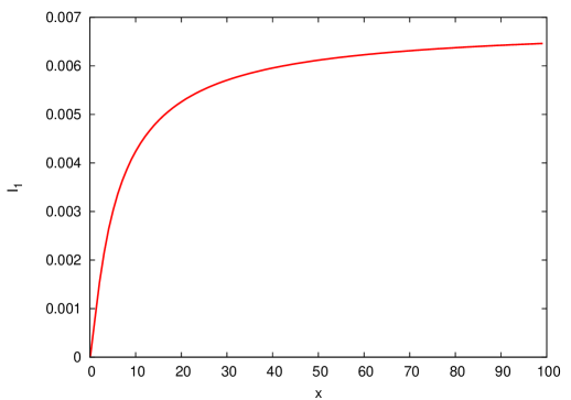
Figure 1: Coefficient function $I_{1}$ as a function of $x={\lambda}_{0}a$. This function reproduces the Casimir result for perfect conducting plates in the limit $x\rightarrow\infty$, $I_{1}(x)\rightarrow\pi^{2}/1440$.

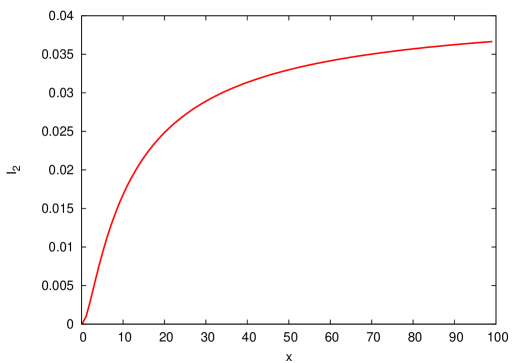
Figure 2: Coefficient function $I_{2}$ as a function of $x={\lambda}_{0}a$. This function approaches $0.0366$ in the limit $x\rightarrow\infty$.

As a second example, we now consider the vacuum energy for the generalized $\delta$-potentials, assuming that the coefficients $\tilde{\mu}_{i}$ do not depend on $\epsilon$. In this situation we obtain

$${\tilde{\cal E}}_{0}=\frac{1}{2}\int\frac{d^{d}k_{\parallel}}{(2\pi)^{d}}\ln\left[1-\frac{(\tilde{\mu}_{0}\tilde{\mu}_{2}-\tilde{\mu}_{1}^{2})^{2}\,e^{-2ak_{\parallel}}}{[(2k_{\parallel}+\tilde{\mu}_{0})\tilde{\mu}_{2}-\tilde{\mu}_{1}^{2}]^{2}}\right]=\frac{1}{2}\int\frac{d^{d}k_{\parallel}}{(2\pi)^{d}}\ln\left[1-\frac{\tilde{\mu}_{eff}^{2}\,e^{-2ak_{\parallel}}}{[2k_{\parallel}+\tilde{\mu}_{eff}]^{2}}\right],$$ (56)

where $\tilde{\mu}_{eff}=(\tilde{\mu}_{0}\tilde{\mu}_{2}-\tilde{\mu}_{1}^{2})/\tilde{\mu}_{2}$. It is interesting to note that the Casimir energy is well defined only when the parameters $\mu_{i}$ are such that the coefficient that multiplies $e^{-2ak_{\parallel}}$ is less than 1, and this is the case if $\tilde{\mu}_{eff}>0$. This condition have been found before, albeit in a different looking but equivalent form; indeed, we have seen that, for the auxiliary field representation (31) to make sense, positivity of the eigenvalues of the matrix ${\bf M}$ is a necessary (and sufficient) condition. From a physical point of view, this condition can be interpreted as follows: the interaction term at each mirror may be diagonalized, to look like the sum of two decoupled quadratic interaction terms, each one involving a mixture of the field and its normal derivative at the mirror. For the vacuum to be stable, one must have therefore non-negative eigenvalues, since they are the coefficients that affect each decoupled term. Vanishing eigenvalues, on the other hand, are not forbidden physically, rather, one should represent them with just one auxiliary field. Otherwise the redundancy pops up in the form of a zero mode.

It is remarkable that Eq.(56) corresponds to the Casimir energy for a usual $\delta$-potential (i.e. without derivatives of the $\delta$-function) with an effective coefficient given by $\tilde{\mu}_{eff}$. However, it is also worth stressing that this equation has been derived assuming a particular regularization for $\Lambda(k_{\parallel})$. While this regularization is well justified in the case of the derivative expansion, a formal calculation which started from the generalized $\delta$-potentials, could give different, regularization dependent results, without any immediate physical reason to chose one from another. For example, in the framework of dimensional regularization one would obtain $\Lambda(k_{\parallel})=\alpha-\frac{k}{2}$, with $\alpha$ an arbitrary constant.

Different regularizations of this object correspond, physically, to imposing different boundary conditions for the propagator of the vacuum field at the mirror. If the concrete model for the finite width mirror is unknown, this lack of information manifests itself in the fact that one has many regularizations available, and they give rise to different values of the energy. However, one knows that, what makes sense physically is not the regularization used; rather, it is the boundary condition it produces on the propagator. Then, one may regard the boundary condition for the propagator as a renormalization condition which hides the ignorance on the details of the model into a bare coefficient function prep .

IV Discussion

We have shown, in concrete examples, how the nonlocal induced action which results from the integration of the microscopic fields (that represent the media composing the mirrors) can be expanded to produce a local action; i.e., one that has point-like support. This means that it may be written as terms involving the $\delta$-function and its derivatives.

Equipped with the general form of that local action, we then derived the Casimir energy for the vacuum scalar field. A conceptually interesting point is that the presence of derivatives of the $\delta$-function, in the effective action, produces a final result for the Casimir energy that can be written in the form of the Lifshitz formula for the electromagnetic field with $2\times 2$ reflection matrices. This analogy is a biproduct of the representation of the effective action in terms of two auxiliary fields

When the coefficients from that local action come from a microscopic model, we have shown that the result may be consistently expanded in powers of the width of the mirrors, producing a result which may be interpreted as a Dirichlet-like energy plus sub-leading corrections. It would be interesting to generalize these results to the realistic case of the electromagnetic field coupled to Dirac fields describing charges on the mirrors.

Besides, we considered also the case when the coefficients are assumed to be independent of the width of the mirrors. In this case, the exact result adopts a quite simple form: the vacuum energy coincides with the one given by the usual $\delta$-potential, with an effective coupling. That is to say, the effect of the terms proportional to derivatives of the $\delta$-function in the effective action is to renormalize the coupling of the usual $\delta$ potential. The last result depends, in principle, on the particular regularization used to handle these (highly singular) potentials. However, when one abandons the description in terms of the coefficients for those terms, in favour of another in terms of the boundary conditions on the propagator, the apparent ambiguity disappears prep .

References

(1)
G. Plunien, B. Müller, and W. Greiner, Phys. Rep. 134,
87 (1986); P. Milonni, The Quantum Vacuum (Academic Press,
San Diego, 1994); V. M. Mostepanenko and N. N. Trunov, The
Casimir Effect and its Applications (Clarendon, London, 1997); M.
Bordag, The Casimir Effect 50 Years Later (World Scientific, Singapore, 1999);
M. Bordag, U. Mohideen, and V. M. Mostepanenko, Phys. Rep.
353, 1 (2001); K. A. Milton, The Casimir Effect:
Physical Manifestations of the Zero-Point Energy (World
Scientific, Singapore, 2001); S. Reynaud et al., C. R. Acad.
Sci. Paris IV-2, 1287 (2001); K. A. Milton, J. Phys. A:
Math. Gen. 37, R209 (2004); S.K. Lamoreaux, Rep. Prog.
Phys. 68, 201 (2005); Special Issue ”Focus on Casimir Forces”,
New J. Phys. 8 (2006).
(2)
C. D. Fosco, F. C. Lombardo and F. D. Mazzitelli,
Phys. Lett. B 669, 371 (2008)
[arXiv:0807.3539 [hep-th]].
(3)
M. Bordag, I. V. Fialkovsky, D. M. Gitman and D. V. Vassilevich,
arXiv:0907.3242 [hep-th].
(4)
C. D. Fosco and E. Losada,
Phys. Lett. B 675, 252 (2009).
(5)
R. Esquivel, C. Villarreal and W. L. Mochán, Phys. Rev. A 68,
052103 (2003);
R. Esquivel-Sirvent, C. Villarreal, W. L. Mochan, A. M. Contreras-Reyes and V. B. Svetovoy,
J. Phys. A 39, 6323 (2006);
A. Saharian and G. Esposito, In the Proceedings of 11th Marcel
Grossmann Meeting on General Relativity, Berlin, Germany, 23-29 Jul 2006,
pp 2761-2763 052103 (2003);
A. Saharian and G. Esposito, J. Phys. A 39, 5233 (2006).
(6)
C. D. Fosco, F. C. Lombardo and F. D. Mazzitelli,
Phys. Rev. D 77, 085018 (2008)
[arXiv:0801.0760 [hep-th]]. See also
I. Fialkovsky, Y. Pis’mak and V. Markov,
Phys. Rev. D 79, 028701 (2009).
(7) M. Bordag, M. Hennig and D. Robaschik, J. Phys. A:Math. Gen25, 4483 (1992).
(8) K. Milton, J. Phys. A: Math. Gen37, 6391 (2004);
K. A. Milton and J. Wagner,
J. Phys. A 41, 155402 (2008)
[arXiv:0712.3811 [hep-th]].
(9) F. S. S. Rosa, D. A. R. Dalvit and P. W. Milonni,
Phys. Rev. A 78, 032117 (2008).
(10) A detailed
explanation of this point will be provided elsewhere:
C. D. Fosco, F. C. Lombardo and F. D. Mazzitelli, in preparation.