Critical Casimir effect in classical binary liquid mixtures

Abstract

If a fluctuating medium is confined, the ensuing perturbation of its fluctuation spectrum generates Casimir-like effective forces acting on its confining surfaces. Near a continuous phase transition of such a medium the corresponding order parameter fluctuations occur on all length scales and therefore close to the critical point this effect acquires a universal character, i.e., to a large extent it is independent of the microscopic details of the actual system. Accordingly it can be calculated theoretically by studying suitable representative model systems. We report on the direct measurement of critical Casimir forces by total internal reflection microscopy (TIRM), with femto-Newton resolution. The corresponding potentials are determined for individual colloidal particles floating above a substrate under the action of the critical thermal noise in the solvent medium, constituted by a binary liquid mixture of water and 2,6-lutidine near its lower consolute point. Depending on the relative adsorption preferences of the colloid and substrate surfaces with respect to the two components of the binary liquid mixture, we observe that, upon approaching the critical point of the solvent, attractive or repulsive forces emerge and supersede those prevailing away from it. Based on the knowledge of the critical Casimir forces acting in film geometries within the Ising universality class and with equal or opposing boundary conditions, we provide the corresponding theoretical predictions for the sphere — planar wall geometry of the experiment. The experimental data for the effective potential can be interpreted consistently in terms of these predictions and a remarkable quantitative agreement is observed.

I Introduction

I.1 Fluctuation-induced forces

At macroscopic scales thermal or quantum fluctuations of a physical property of a system are typically negligible because fluctuations average out to zero upon increasing the length and time scales at which the system is studied. At the micro- and nano-meter scale, instead, fluctuations become generally relevant and, if externally controlled and spatially confined, they give rise to novel phenomena. An example thereof is provided by the Casimir force acting on conducting bodies Casimir , which is due to the confinement of quantum fluctuations of the electromagnetic field in vacuum and which influences the behavior of micrometer-sized systems ranging from colloids to micro- and nano-electromechanical systems (MEMS, NEMS).

Thermal fluctuations in condensed matter typically occur on a molecular scale. However, upon approaching the critical point of a second-order phase transition the fluctuations of the order parameter $\phi$ of the phase transition become relevant and detectable at a much larger length scale $\xi$ and their confinement results in a fluctuation-induced Casimir force $f_{\mathrm{C}}$ acting on the confining surfaces FdG . This so-called critical Casimir force $f_{\mathrm{C}}$ has a range which is set by the correlation length $\xi$ of the fluctuations of the order parameter. Since near the critical point $\xi$ can reach up to macroscopic values, the range of $f_{\mathrm{C}}$ can be controlled and varied to a large extent by minute temperature changes close to the critical temperature $T_{c}$. We shall show that this control of the thermodynamic state of the system is a manageable task. This implies that the critical Casimir force can be easily switched on and off, which allows one to identify it relative to the omnipresent background forces. In addition, by proper surface treatments of the confining surfaces, the force can be relatively easily turned from attractive to repulsive krech:99:0 ; Dbook in contrast to the Casimir force stemming from electromagnetic fluctuations for which such a change requires carefully chosen bulk materials providing the solid walls and the fluid in between Cap:2009 . Such a repulsive force might be exploited to prevent stiction in MEMS and NEMS, which would open significant perspectives for applications. Finally, at $T_{c}$ the strength of the critical Casimir force can easily compete with or even dominate dispersion forces, with which it shows the same algebraic decay, however without suffering from the weakening due to retardation effects. The universality of $f_{\mathrm{C}}$ means that the same force is generated near the critical point of liquid-vapor coexistence of any fluid or near the consolute point of phase segregation of any binary or multicomponent liquid mixture. This allows one to pick and use those representatives of the universality class which in addition optimize desired performances of MEMS and NEMS. This provides a highly welcome flexibility.

The fluctuation-induced forces generated by confining the fluctuations of electromagnetic fields in the quantum vacuum (Casimir effect) or of the order parameter in a critical medium (critical Casimir effect) have a common description within the field-theoretical approach. Accordingly, the connection between these two effects goes well beyond the mere analogy and it indeed becomes an exact mapping in some specific cases of spatial dimension $d$, geometries, and boundary conditions. This deep connection actually justifies the use of the term “critical Casimir force” when referring to the effective force due to the confinement of critical fluctuations. On the other hand, from a theoretical point of view the quantum and the critical Casimir effect are also distinct in that the quantum one in vacuum corresponds to a free field theory whereas the critical one is described by a more challenging non-Gaussian field theory.

I.2 Finite-size scaling

The theory of finite-size scaling (see, e.g., Refs. krech:99:0 ; Dbook ) predicts that in the vicinity of $T_{c}$ the critical Casimir force $f_{\mathrm{C}}$ and its dependence on temperature are described by a universal scaling function which depends only on the gross features of the system and of the confining surfaces, i.e., on the so-called universality class of the phase transition occurring in the bulk and on the geometry and surface universality classes of the confining surfaces Binder83 ; diehl:86:0 ; diehl:97 . The latter characterize the boundary conditions (BC) Binder83 ; diehl:86:0 ; diehl:97 ; krech:99:0 the surfaces impose on the fluctuations of the order parameter of the underlying second-order phase transition. The actual physical nature of the order parameter $\phi$ depends on which kind of continuous phase transition is approached: in the case we shall be mainly concerned with in the following, i.e., the consolute point of phase segregation in binary liquid mixtures, $\phi$ is given by the difference between the local and the mean concentration of one of the two components of the mixture (see, c.f., Sec. III.2 for further details). For binary liquid mixtures the confining surfaces generically exhibit preferential adsorption of one of the two components of the mixture, resulting in an enhancement of the order parameter $\phi$ close to the surface. (This amounts to the presence of symmetry-breaking surface fields, see, e.g., Refs. Binder83 ; diehl:86:0 ; diehl:97 .) One usually refers to the corresponding boundary conditions as $(+)$ or $(-)$ depending on whether the surface favors $\phi>0$ or $\phi<0$, respectively. Due to its universal nature, the critical Casimir force can be studied via representative models which are amenable to theoretical investigations. Since due to universality microscopic details can only in a rather limited way be blamed for potential discrepancies, the resulting predictions face very stringent experimental tests.

Most of the available theoretical and experimental studies focus on the film geometry in which the system undergoing the second-order phase transition is confined between two parallel surfaces of large transverse area $S$ at a distance $L$. For this geometry and assuming that the only relevant thermodynamic variable is the temperature $T$ (possible additional variables such as the concentration are set to their critical values), renormalization-group theory shows krech:92a ; krech:92b that the critical Casimir force $f_{\mathrm{C}}$ scales as

$$\frac{f_{\mathrm{C}}(T,L)}{k_{\mathrm{B}}T}=\frac{S}{L^{3}}\vartheta(\tau(L/\xi^{+}_{0})^{1/\nu})$$ (1)

in three spatial dimensions ($d=3$), where $\vartheta(x)$ is a universal scaling function, and $\tau$ is the reduced deviation from the critical temperature $T_{c}$ such that $\tau>0$ corresponds to the disordered (homogeneous) phase. If, as it is usually the case, the homogeneous phase is located at high temperatures in the phase diagram of the system, one defines $\tau=(T-T_{c})/T_{c}$. However, there are also cases – such as the one we shall be interested in (see, c.f., Fig. 8) – in which this phase is located at low temperatures so that there one defines $\tau=-(T-T_{c})/T_{c}$. The system-specific (i.e., non-universal) amplitudes $\xi_{0}^{\pm}$ in Eq. (1) enter into the algebraic behavior of the bulk correlation length $\xi$ of the order parameter $\phi$ upon approaching the critical point:

$$\xi(\tau\rightarrow 0^{\pm})=\xi^{\pm}_{0}|\tau|^{-\nu}\;.$$ (2)

In what follows we shall mainly consider $\xi_{0}\equiv\xi_{0}^{+}$, which forms with $\xi_{0}^{-}$ a universal amplitude ratio $U_{\xi_{\rm gap}}\equiv\xi_{0}^{+}/\xi_{0}^{-}\simeq 1.9$ PV ; Priv in those cases in which $\xi(\tau<0)$ is finite. (Renormalization-group theory tells that in the bulk there are only two independent non-universal amplitudes, say $\xi_{0}^{+}$ and $C_{\phi}=\langle\phi\rangle/(-\tau)^{\beta}$ of the order parameter below $T_{c}$; all other non-universal amplitudes can be expressed in terms of them and universal amplitude ratios Priv . Here $\beta$ is the critical exponent which characterizes the singular behavior $\langle\phi\rangle\sim(-\tau)^{\beta}$ of the average order parameter $\langle\phi\rangle$ for $\tau\rightarrow 0^{-}$, with $\beta=0.3265(3)$ for the three-dimensional Ising universality class PV .) The bulk correlation length $\xi$ can be inferred from, e.g., the exponential decay of the two-point correlation function of the order parameter. The algebraic increase of $\xi$ [Eq. (2)] is characterized by the universal exponent $\nu$ which equals $0.6301(4)$ for the three-dimensional Ising universality class PV which captures, among others, the critical behavior of binary liquid mixtures close to the demixing point as studied experimentally here.

I.3 Theoretical predictions and previous experiments

For the Ising universality class with symmetry-breaking boundary conditions theoretical predictions for the universal scaling function $\vartheta$ are available from field-theoretical krech ; upton and Monte Carlo studies krech ; vas-07 ; vas-08 . The critical Casimir force turns out to be attractive for equal boundary conditions (BC) on the two surfaces, i.e., ${(+,+)}$ or ${(-,-)}$, whereas it is repulsive and generically stronger for opposing boundary conditions, i.e., ${(+,-)}$ or ${(-,+)}$. In the presence of such boundary conditions, for topographically patt-top or chemically patt-chem patterned confining surfaces or for curved surfaces colloids1a ; colloids1b theoretical results are available primarily within mean-field theory.

Following theoretical predictions and suggestions krech:92c , previous indirect evidences for both attractive and repulsive critical Casimir force were based on studying fluids close to critical endpoints (see Ref. gam-08 for a more detailed summary). Under such circumstances, the film geometry with parallel planar walls can be indeed experimentally realized by forming complete wetting fluid films diet:98 in which a liquid phase is confined between a solid substrate (or another spectator phase) and the interface with the vapor phase and its thickness $L$ can be tuned by undersaturation, in particular off criticality. Upon changing pressure and temperature one can drive the liquid film towards a second-order phase transition which nonetheless keeps the confining liquid-vapor interface sharp. The fluctuations of the associated order parameter, confined within the film of thickness $L$, give rise to a critical Casimir pressure (related to $\vartheta$ krech:92c ) which acts on the liquid-vapor interface, displacing it from the equilibrium position it would have under the effect of dispersion forces alone, i.e., in the absence of critical fluctuations. This results in a temperature-dependent change of $L$. Based on the knowledge of the relationship between $L$ and pressure, by monitoring this variation it is possible to infer indirectly the magnitude of the Casimir force which drives this change of thickness. This approach has been used for the study of wetting films of ⁴He at the normal-superfluid transition garcia4 , for ³He-⁴He mixtures close to the tricritical point garcia3 , and for classical binary liquid mixtures close to demixing transitions pershan ; rafai . The film thickness $L$ has been determined by using capacitance garcia4 ; garcia3 or X-ray reflectivity measurements pershan , or ellipsometry rafai . For the results of Refs. garcia4 , garcia3 , and pershan the quantitative agreement with the theoretical predictions for the corresponding bulk and surface universality classes (see Refs. krech:92a ; krech:92b ; krech:92c ; vas-07 ; vas-08 ; hucht ; hasen ; DK ; kardar:04 ; LGW-MFa ; LGW-MFb , LGW-MFa ; MD:06 , and upton ; vas-07 ; vas-08 ; LGW-MFa , respectively) are excellent garcia4 or remarkably good garcia3 ; pershan . For ⁴He garcia4 one has Dirichlet-Dirichlet boundary conditions, for ³He-⁴He mixtures garcia3 Dirichlet-$(+)$ boundary conditions, and in Ref. pershan ${(+,-)}$ boundary conditions hold.

I.4 Direct determination of critical Casimir forces

The aim of the experimental investigation discussed here is to provide a direct determination of the Casimir force, by measuring the associated potential $\Phi_{C}$. On dimensional grounds and on the basis of Eq. (1), the scale of this potential is set by $k_{\mathrm{B}}T_{c}$ and therefore, as realized in Ref. pershan , in order to enhance the strength of the critical Casimir force it is desirable to engage critical points with higher $T_{c}$ compared to those of the $\lambda$-transition investigated in Refs. garcia3 ; garcia4 . This consideration suggests classical fluids as natural candidates for the critical medium. The experimentally driven preference for having $T_{c}$ and the critical pressure to be close to ambient conditions can be satisfied by numerous binary liquid mixtures which exhibit consolute points for phase segregation. From Eq. (1) one can infer a rough estimate of the critical Casimir force $f_{\mathrm{C}}$. For an object which exposes an effective area $S=1\,\mu\mbox{m}^{2}$ to a wall at a distance $L=100\,\mbox{nm}$, and for $T_{c}=300\,\mbox{K}$ one finds $f_{\mathrm{C}}\lesssim 4\,\mbox{pN}$. Since the scaling function $\vartheta(x)$ vanishes upon moving away from criticality, i.e., $\vartheta(|x|\rightarrow\infty)\rightarrow 0$, and because one is interested in probing also larger distances $L$, one needs force measurements with a force resolution which is significantly better than pN. Atomic force microscopy at room temperature cannot deliver fN accuracy. This required sensitivity can, however, be achieved by using total internal reflection microscopy (TIRM), which enables one to determine the potential of the effective forces acting on a colloidal particle near a wall, by monitoring its Brownian motion in a solvent. Choosing as the solvent a suitable binary liquid mixture allows one to investigate the critical Casimir force on the particle which arises upon approaching the demixing transition of the mixture. Such a second-order phase transition falls into the bulk universality class of the Ising model. In this geometrical setting the fluctuation spectrum of the critical medium (i.e., the binary liquid mixture) is perturbed by the confinement due to a flat wall and by the presence of the spherical cavity. The curvature of one of the two confining surfaces introduces an additional length scale and thus leads to an extension of the scaling form in Eq. (1) such that the scaling function $\vartheta$ additionally depends on the ratio between the radius $R$ of the colloid and the minimal distance $z$ between the surface of the colloid and the flat surface of the substrate [c.f., Sec. II.1; here $z$ plays the role of $L$ in Eq. (1)]. At present, for arbitrary values of $z$ and radii of curvature, theoretical predictions for the critical Casimir force in a geometrical setting involving one non-planar surface are available only within mean-field theory, both for spherical colloids1a ; colloids1b and ellipsoidal khd-08 particles, which demonstrate that the results of the so-called Derjaguin approximation are valid for $z/R\ll 1$ colloids1a ; colloids1b (see, c.f., Sec. II). Beyond mean-field theory and for various universality classes, theoretical results have been obtained in the so-called protein limit corresponding to $z/R$, $\xi/z\gg 1$ eisen ; krech:92a where $R$ indicates the typical size of the, in general nonspherical, particle. However, at present this protein limit is not accessible by TIRM because for small particles far away from the substrate (through which the evanescent optical field enters into the sample) the signal of the scattered light from the particle is too weak. The experimentally relevant case is the opposite one of a large colloidal particle close to the wall. Although in $d=3$ theoretical results for the full scaling function of the sphere-plate geometry are not available, in this latter case one can take advantage of the Derjaguin approximation in order to express the critical Casimir force $F_{\mathrm{C}}$ acting on the colloid in terms of the force acting within a film geometry, which was investigated successfully via Monte Carlo simulations in Refs. vas-07 ; vas-08 . This is explained in detail in Sec. II.1, in which we present the theoretical predictions for the scaling function of the critical Casimir force (and of the associated potential) for the case of a sphere near a wall immersed into a binary liquid mixture at its critical composition. On the other hand, in Sec. II.2 we discuss the expected behavior of the effective potential of the colloid if the binary liquid mixture is not at its critical concentration so that, upon changing the temperature, it undergoes a first-order phase transition. The discussions in Sec. II form the basis for the interpretation of the experimental results. The experimental setting is described in Sec. III. In Sec. III.1 we recall the principles of TIRM and of the data analysis, whereas in Sec. III.2 we discuss the specific choice of the binary mixture used here and how one can experimentally realize the various boundary conditions. In Sec. IV we present in detail the experimental results, comparing them with the theoretical predictions, for mixtures both at critical and non-critical compositions. A summary and a discussion of perspectives and of possible applications of our findings are provided in Sec. V. Part of the analysis presented here has been reported briefly in Ref. nature . (For a pedagogical introduction to the subject see Ref. EPN .)

II Theoretical predictions

II.1 Critical composition

II.1.1 General properties

The critical Casimir force $F_{\mathrm{C}}$ acting on a spherical particle of radius $R$, at a distance $z$ of closest approach from the flat surface of a substrate and immersed in a near-critical medium at temperature $T\simeq T_{c}$ takes, for strong preferential adsorption, the universal scaling form colloids1a ; colloids1b ; colloids2

$$F_{\mathrm{C}}(z)=\frac{k_{\mathrm{B}}T}{R}K_{\pm}^{\rm(s,p)}\left(x\equiv\frac{z}{\xi},\Delta\equiv\frac{z}{R}\right)\,.$$ (3)

The scaling function $K_{\pm}^{\rm(s,p)}(x,\Delta)$ depends, in addition, on the combination of (sphere, plate) [(s,p)] boundary conditions imposed by the surfaces of the sphere and of the plate and on the phase from which the critical point is approached (i.e., on the sign of $\tau$, with $K_{\pm}^{\rm(s,p)}$ corresponding to $\tau\gtrless 0$). (In line with Eq. (2) and with the standard notation in the literature, the one-phase region is denoted by $+$ and the two-phase region by $-$. These signs should not be confused with the signs ${(+,+)}$ etc. indicating, also in line with the literature, the character of the boundary conditions of the two confining surfaces (s,p). In order to avoid a clumsy notation we suppress or use these two notations in a selfevident way.) The scaling form of the associated potential $\Phi_{C}(z)\equiv\int_{z}^{\infty}\!\!{\rm d}s\;F_{\mathrm{C}}(s)$ follows by integration of Eq. (3). In the two limiting cases $\Delta\gg 1$ and $\Delta\ll 1$ it is possible to calculate $K(x,\Delta)$ on the basis of the so-called small-sphere expansion and Derjaguin approximation, respectively colloids1a ; colloids1b ; colloids2 . In the former case one finds in three space dimensions, for $\tau>0$ and symmetry-breaking boundary conditions ${\rm(s,p)}=(\pm,+)$ (see Eq. (7) in Ref. colloids1a , which also includes higher-order terms)

$$\begin{split}K_{+}^{(\pm,+)}(x,\Delta\rightarrow\infty)=&\mp\frac{a}{c_{+}}\frac{x^{\beta/\nu+1}}{2^{\beta/\nu}}P_{+}^{\prime}(x)\Delta^{-(\beta/\nu+1)}\\ &+O(\Delta^{-2\beta/\nu-1})\,,\end{split}$$ (4)

where $\beta/\nu\simeq 0.518$. In this limit, the force acting on the “small” particle is determined, to leading order, by the interaction between the particle and the average order parameter profile $\langle\phi(z)\rangle_{\infty/2}$ induced by the planar wall in the absence of the particle, i.e., in a semi-infinite system ($\infty/2$). This profile is characterized for $\tau>0$ by the universal scaling function $P_{+}$ entering Eq. (4): $\langle\phi(z)\rangle_{\infty/2}=\langle\phi\rangle_{\infty,-\tau<0}P_{+}(z/\xi)$, where $\langle\phi\rangle_{\infty,-\tau<0}=C_{\phi}\tau^{\beta}$ is the value of the order parameter in the bulk ($\infty$) corresponding to the reduced temperature $-\tau\rightarrow 0^{-}$. The universal constant $c_{+}$ in Eq. (4) characterizes the critical adsorption profile $P_{+}(x\rightarrow 0)\rightarrow c_{+}x^{-\beta/\nu}$, whereas $a=A_{\phi}^{2}/B_{\phi}$ is the universal ratio colloids2 between the non-universal amplitudes $A_{\phi}$ and $B_{\phi}$ of the critical order parameter profile in the semi-infinite system $\langle\phi(z)\rangle_{\infty/2,\tau=0}=A_{\phi}(2z)^{-\beta/\nu}$ and of the two-point correlation function in the bulk $\langle\phi({\bf r})\phi(0)\rangle_{\infty,\tau=0}=B_{\phi}r^{-2\beta/\nu}$, respectively. In turn, $A_{\phi}$ (and therefore $B_{\phi}$) can be expressed in terms of the two independent non-universal amplitudes $\xi_{0}^{+}$ and $C_{\phi}$ via $A_{\phi}=c_{+}C_{\phi}/(2\xi_{0}^{+})^{-\beta/\nu}$. (For a detailed discussion of the values of these universal amplitude ratios we refer the reader to Refs. colloids1a ; colloids1b ; colloids2 .)

II.1.2 Derjaguin approximation

Equation (4) is useful to discuss the behavior of colloids which are small compared to their distance from the plate. However, in the experiment discussed in Sec. III, the distance $z$ is typically much smaller than the radius $R$ of the particle. This case can be conveniently discussed within the Derjaguin approximation, which yields in three dimensions colloids1a

$$K(x,\Delta\rightarrow 0)=\Delta^{-2}\hat{\vartheta}(x)\,,$$ (5)

where the expression for $\hat{\vartheta}(x)$ is determined further below in terms of the scaling function $\vartheta$ of the critical Casimir force $f_{\mathrm{C}}$ acting within a film [see Eq. (1)].

The scaling functions $\vartheta_{{(+,-)}}(x)$ and $\vartheta_{{(+,+)}}(x)$ for the boundary conditions ${(+,-)}$ and ${(+,+)}$ relevant to the study of the critical properties of binary liquid mixtures at their critical compositions have been determined by Monte Carlo simulations vas-07 ; vas-08 . Within the Derjaguin approximation, valid for $\Delta\ll 1$, i.e., if the radius $R$ of the colloid is much larger than the minimal separation $z$ between the surface of the colloid and the flat substrate, the curved surface of the colloid is considered to be made up of successive circular rings of infinitesimal area ${\rm d}S(\theta)$ and radius $r(\theta)$ which are parallel to the substrate and are at a normal distance $L(\theta)=z+R(1-\cos\theta)$ from an opposing identical circular ring on the surface of the substrate (see Fig. 1).

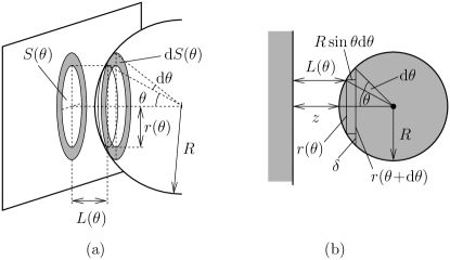
Figure 1: (a) Geometry of the Derjaguin approximation for the plate-sphere geometry, (b) cross section through the center of the sphere and normal to the plate. In (a), the base of a cap of the sphere with radius $r(\theta)$ is shown as a thin line. The inner circle of the grey ring ${\rm d}S(\theta)$ is this thin line shifted by $R\sin\theta{\rm d}\theta$ towards the center of the sphere. In (b), $\delta=r(\theta+{\rm d}\theta)-r(\theta)$ is the cross section of the grey ring ${\rm d}S(\theta)$ shown in (a).

Assuming additivity, the contribution ${\rm d}F_{\mathrm{C}}$ of each single pair of rings to the total Casimir force $F_{\mathrm{C}}$ is given by

$$\frac{{\rm d}F_{\mathrm{C}}}{k_{\mathrm{B}}T}=\frac{{\rm d}S(\theta)}{L^{3}(\theta)}\vartheta(L(\theta)/\xi)$$ (6)

where $\vartheta$ is the scaling function of the critical Casimir force acting within the film geometry [see Eq. (1)]. Here it is convenient to express $\vartheta$ not as a function of $u\equiv\tau(L/\xi_{0})^{1/\nu}$ as in Eq. (1) but as a function of $x=L/\xi$ where $x=u^{\nu}$ for $u>0$ and $x=U_{\xi_{\rm gap}}(-u)^{\nu}$ for $u<0$ with $U_{\xi_{\rm gap}}\simeq 1.9$ PV for the three-dimensional Ising universality class we are interested in. The radius $r(\theta)$ of the ring is given by $r(\theta)=R\sin\theta$ and therefore its area is ${\rm d}S(\theta)=\pi[r(\theta+{\rm d}\theta)]^{2}-\pi[r(\theta)]^{2}=2\pi R^{2}\sin\theta\cos\theta\,{\rm d}\theta$. The total force $F_{\mathrm{C}}$ is obtained by summing all the contributions ${\rm d}F_{\mathrm{C}}(\theta)$ of the circular rings, up to the maximal angle $\theta_{\rm M}$

$$\frac{F_{\mathrm{C}}}{k_{\mathrm{B}}T}=\int_{\theta=0}^{\theta_{\rm M}}\;\frac{{\rm d}S(\theta)}{L^{3}(\theta)}\vartheta(L(\theta)/\xi)\,.$$ (7)

$\theta_{\rm M}=\pi/2$ is a natural choice, neglecting any influences from the back side of the sphere. However, we shall see below that its specific value does not affect the result in the limit $R\gg z$. For $R\gg z$ the integral (due to the denominator) is dominated by the contributions it picks up at small angle $\theta$, so that one can approximate $L(\theta)/z\simeq 1+(R/z)(\theta^{2}/2)$ and therefore

$$\frac{F_{\mathrm{C}}(z)}{k_{\mathrm{B}}T}=\frac{2\pi R^{2}}{z^{3}}\int_{0}^{\theta_{\rm M}}{\rm d}\theta\;\frac{\theta}{\left[1+\frac{R}{z}\theta^{2}/2\right]^{3}}\vartheta([1+\frac{R}{z}\theta^{2}/2]z/\xi)\,.$$ (8)

[For $\theta_{\rm M}\rightarrow\infty$ this is identical with Eq. (4) in Ref. colloids1a .] Introducing the variable $l=1+(R/z)(\theta^{2}/2)$, one can write the previous expression as

$$\frac{F_{\mathrm{C}}(z)}{k_{\mathrm{B}}T}=\frac{2\pi R}{z^{2}}\int_{1}^{l_{\rm M}}{\rm d}l\;\frac{1}{l^{3}}\vartheta(l\,z/\xi)$$ (9)

where $l_{\rm M}\equiv 1+(R/z)(\theta_{\rm M}^{2}/2)$. In the limit $R/z\rightarrow\infty$, $l_{\rm M}\rightarrow\infty$ independently of $\theta_{\rm M}$, so that the integral can be extended up to $\infty$ and

$$\frac{F_{\mathrm{C}}(z)}{k_{\mathrm{B}}T}=\frac{R}{z^{2}}\hat{\vartheta}(z/\xi)$$ (10)

where

$$\hat{\vartheta}(x)=2\pi\int_{1}^{\infty}{\rm d}l\;\frac{1}{l^{3}}\vartheta(l\,x).$$ (11)

The potential $\Phi_{C}(z)$ associated with the Casimir force is given by

$$\begin{split}\frac{\Phi_{C}(z)}{k_{\mathrm{B}}T}&=\frac{2\pi R}{z}\int_{1}^{\infty}\!\!{\rm d}y\int_{1}^{\infty}\!\!{\rm d}l\;y^{-2}l^{-3}\vartheta(ly\,z/\xi)\\ &=\frac{R}{z}\;2\pi\int_{1}^{\infty}{\rm d}v\left(\frac{1}{v^{2}}-\frac{1}{v^{3}}\right)\vartheta(v\,z/\xi)\\ &=\;\frac{R}{z}\;\Theta(z/\xi)\end{split}$$ (12)

where we have changed the variable $l\mapsto v\equiv ly$, exchanged the order of the remaining integrals $\int_{1}^{\infty}{\rm d}y\int_{y}^{\infty}{\rm d}v=\int_{1}^{\infty}{\rm d}v\int_{1}^{v}{\rm d}y$, and introduced the scaling function

$$\Theta(x)\equiv 2\pi\int_{1}^{\infty}{\rm d}v\left(\frac{1}{v^{2}}-\frac{1}{v^{3}}\right)\vartheta(v\,x)\,.$$ (13)

According to Eqs. (10) and (12), for separations $z$ much smaller than the radius of the colloid, the Casimir force and the Casimir potential increase linearly upon increasing the radius $R$ of the colloid. At the bulk critical point, $\hat{\vartheta}(0)=\Theta(0)=\pi\vartheta(0)$ and $\hat{\vartheta}^{\prime}(0)=2\pi\vartheta^{\prime}(0)$, whereas $\Theta^{\prime}(0)=\infty$. If in the film geometry the force is attractive (repulsive) at all temperatures, within the Derjaguin approximation the same sign holds also in the sphere-plate geometry. At the critical concentration the Casimir force acting on a $(+)$ colloid in front of a $(-)$ substrate is the same as the one acting on a $(-)$ colloid in front of a $(+)$ substrate. This is no longer true for non-critical concentrations. Although the Derjaguin approximation is expected to be valid only for $R\gg z$, the comparison between the results of the mean-field calculation colloids1a ; colloids1b for the actual sphere-plate geometry and the ones of the corresponding Derjaguin approximation based on the mean-field theory (MFT) for the film geometry show good agreement even for $z/R$ up to $0.4\div 0.5$.

II.1.3 Theoretical predictions for scaling functions

For the universality class of the three-dimensional Ising model, the scaling functions $\vartheta$ for the Casimir force in the film geometry – which enter into Eq. (13) – have been determined in Refs. vas-07 ; vas-08 for ${(+,+)}$ and ${(+,-)}$ BC (or, equivalently, ${(-,-)}$ and ${(-,+)}$ BC) by Monte Carlo simulations. Due to the presence of strong corrections to scaling, the amplitudes of the corresponding numerical estimates for $\vartheta_{(+,+)}(x)$ and $\vartheta_{(+,-)}(x)$ are affected by a systematic uncertainty of about 20% vas-07 ; vas-08 . The numerical data presented in Refs. vas-07 ; vas-08 are very well fitted by certain analytic ansätze (at least in the range of scaling variable which has been investigated numerically) which, in turn, can be used in order to calculate the corresponding scaling functions $\Theta_{(+,+)}$ and $\Theta_{(+,-)}$ for the potential (Fig. 2, see also Fig. 2(d) in Ref. nature ) as well as $\hat{\vartheta}_{(+,+)}$ and $\hat{\vartheta}_{(+,-)}$ for the force (Fig. 3). The simulation data for the film scaling functions $\vartheta_{(+,+)}(x)$ and $\vartheta_{(+,-)}(x)$ can actually be fitted even by functions of various shapes (the asymptotic behavior of which for large $|x|$ is, however, fixed, see further below). This leads to different estimates of the scaling functions outside the range of the scaling variable for which the Monte Carlo data are currently available. This results also in different estimates of $\Theta_{(+,+)}$, $\Theta_{(+,-)}$, $\hat{\vartheta}_{(+,+)}$, and $\hat{\vartheta}_{(+,-)}$ obtained from $\vartheta_{(+,+)}(x)$ and $\vartheta_{(+,-)}(x)$ via Eqs. (13) and (11). However, the uncertainty of the estimates for the shapes is negligible compared to the inherent systematic uncertainty associated with the amplitudes of $\vartheta_{(+,+)}(x)$ and $\vartheta_{(+,-)}(x)$. For a detailed discussion of these issues we refer to Ref. vas-08 .

The critical Casimir force $f_{\mathrm{C}}(T,L)$ between two planar walls [see Eq. (1)] with symmetry-breaking boundary conditions is expected to vary as $\exp(-L/\xi)$ as a function of $L\gg\xi$ for $\tau>0$ (see, e.g., Ref. Tr-09 and in particular the footnote Ref. [23] therein). Accordingly, $\vartheta_{(+,\pm)}(x\gg 1)=A_{\pm}\,x^{3}{\rm e}^{-x}$ and from Eqs. (11) and (13) one finds

$$\begin{split}\hat{\vartheta}_{(+,\pm)}(x\gg 1)&=2\pi A_{\pm}\,x^{2}\,{\rm e}^{-x}\quad\mbox{and}\\ \Theta_{(+,\pm)}(x\gg 1)&=2\pi A_{\pm}\,x\,{\rm e}^{-x},\end{split}$$ (14)

for the critical Casimir force and potential, respectively, in the sphere-plate geometry. The analysis of the Monte Carlo data presented in Figs. 9 and 10 of Ref. vas-08 yields $A_{+}^{(i)}=-1.51(2)$ and $A_{-}^{(i)}=1.82(2)$, respectively, for the data sets therein indicated as $(i)$ whereas it yields $A_{+}^{(ii)}=-1.16(2)$ and $A_{-}^{(ii)}=1.38(2)$ for the corresponding data set $(ii)$. (We recall here that the data sets $(i)$ and $(ii)$ turn out to be proportional to each other, see Refs. vas-07 ; vas-08 for details.)

Figure 3 shows that the critical Casimir force for the sphere-plate geometry exhibits the same qualitative features as in the film geometry: For ${(+,+)}$ [${(+,-)}$] BC the force is attractive (repulsive) and attains its maximum strength for $\tau>0$ ($\tau<0$), corresponding to the one-phase (two-phase) region. For fixed values of the scaling variable, the strength of the repulsive force for ${(+,-)}$ BC is larger than the one of the attractive force in the case of ${(+,+)}$ BC. The inset of Fig. 3 compares the estimate for the scaling function $\hat{\vartheta}_{{(+,+)}}(x=L/\xi)$ — up to its normalization $\hat{\vartheta}_{{(+,+)}}(0)$ — based on the Monte Carlo data of Refs. vas-07 ; vas-08 (solid line) with the early estimate of Ref. colloids1a , which is based on the pointwise and linear interpolation between the exactly known film scaling functions in $d=2$ and $d=4$, such as to obtain an estimate of $\hat{\vartheta}_{{(+,+)}}(x=L/\xi)$ for $d=3$ (dashed line). Although this latter estimate captures correctly some qualitative features of the universal scaling function $\hat{\vartheta}_{{(+,+)}}(x=L/\xi)$, it fails to be quantitatively accurate, as the comparison with the Monte Carlo estimate reveals. The same consideration applies to the corresponding estimates for $\Theta_{{(+,+)}}$.

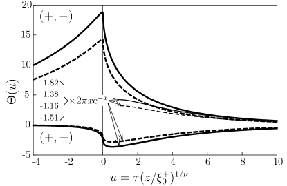
Figure 2: Scaling functions $\Theta_{(+,+)}$ and $\Theta_{(+,-)}$ of the Casimir potential $\Phi_{C}$ [see Eq. (12)] for ${(+,+)}$ and ${(+,-)}$ BC, respectively, within the Derjaguin approximation and for the three-dimensional Ising universality class, as functions of $u=\tau(z/\xi_{0}^{+})^{1/\nu}$ with $\nu\simeq 0.630$. The thick solid and dashed lines have been obtained via Eq. (13) on the basis of the Monte Carlo estimates for $\vartheta_{{(+,+)},{(+,-)}}$ presented in Refs. vas-07 ; vas-08 , indicated by $(i)$ and $(ii)$, respectively, in Figs. 9 and 10 of Ref. vas-08 . (The thick solid lines agree with the estimates reported in Fig. 2(d) of Ref. nature .) $\Theta_{{(+,+)}}$ attains its minimum value $\Theta_{{(+,+)}}^{\rm(min)}\simeq-3.6$ (solid line) and $-2.8$ (dashed line) both for $u_{\rm min}\simeq 0.54$, whereas $\Theta_{{(+,-)}}$ attains (smoothly) its maximum value $\Theta_{{(+,-)}}^{\rm(max)}\simeq 19$ (solid line) and $14$ (dashed line) both for $u_{\rm min}\simeq-0.03$. The first derivatives of $\Theta_{{(+,-)}}$ and $\Theta_{{(+,+)}}$ diverge logarithmically for $u\rightarrow 0$. The thin lines for $u>1$ indicate the asymptotic behaviors of $\Theta(u\gg 1)$ given in Eq. (14) with the numerical values of the coefficients $A_{\pm}$ indicated from top to bottom for the corresponding curves. For ${(+,+)}$ boundary conditions the asymptotic expressions are indistinguishable from $\Theta_{{(+,+)}}(u)$ for $u\gtrsim 4$.

Equations (12) and (13), together with Fig. 2, form the theoretical basis for the interpretation of the experimental results for the effective interaction potential between a spherical colloidal particle and a planar wall, immersed into a binary liquid mixture at its critical composition and near its consolute point.

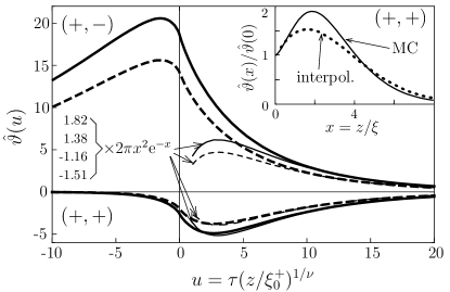
Figure 3: Scaling functions $\hat{\vartheta}_{(+,+)}$ and $\hat{\vartheta}_{(+,-)}$ of the Casimir force $F_{C}$ [see Eq. (10)] for ${(+,+)}$ and ${(+,-)}$ BC, respectively, within the Derjaguin approximation and for the three-dimensional Ising universality class, as functions of $u=\tau(z/\xi_{0}^{+})^{1/\nu}$ with $\nu\simeq 0.630$. The thick solid and dashed lines have been obtained via Eq. (11) on the basis of the Monte Carlo estimates for $\vartheta_{{(+,+)},{(+,-)}}$ presented in Refs. vas-07 ; vas-08 , indicated by $(i)$ and $(ii)$, respectively, in Figs. 9 and 10 of Ref. vas-08 . $\hat{\vartheta}_{{(+,+)}}$ attains its minimum value $\hat{\vartheta}_{{(+,+)}}^{\rm(min)}\simeq-4.9$ (solid line) and $-3.8$ (dashed line) both for $u_{\rm min}\simeq 2.6$, whereas $\hat{\vartheta}_{{(+,-)}}$ attains its maximum value $\hat{\vartheta}_{{(+,-)}}^{\rm(max)}\simeq 21$ (solid line) and $16$ (dashed line) both for $u_{\rm min}\simeq-1.5$. The second derivatives of $\hat{\vartheta}_{(+,+)}(u)$ and $\hat{\vartheta}_{(+,-)}(u)$ diverge logarithmically for $u\rightarrow 0$. The thin lines for $u>1$ indicate the asymptotic behaviors $\hat{\vartheta}(u\gg 1)$ given in Eq. (14) with the numerical values of the coefficients $A_{\pm}$ indicated from top to bottom for the corresponding curves. For ${(+,+)}$ boundary conditions the asymptotic expressions are indistinguishable from $\hat{\vartheta}_{{(+,+)}}(u)$ for $u\gtrsim 5$. In the inset we compare the estimate for $\hat{\vartheta}_{(+,+)}(x)/\hat{\vartheta}_{(+,+)}(0)$ as a function of $x=z/\xi$ based on the Monte Carlo data of Refs. vas-07 ; vas-08 (solid line, MC) with the one presented in Ref. colloids1a and obtained by interpolating linearly and pointwise the exactly known film scaling functions in $d=2$ and $d=4$ in order to obtain an estimate for $d=3$ (dotted line, interpol.). The Monte Carlo estimate for this ratio is the same for both data sets $(i)$ and $(ii)$ in Ref. vas-08 .

II.1.4 Deviations from strong adsorption

The theoretical analyses presented above and in Refs. vas-07 ; vas-08 ; nature assume that the confining surfaces are characterized by a sufficiently strong preferential adsorption for one of the two components of the mixture, corresponding to $(+)$ or $(-)$ fixed-point boundary conditions in the sense of renormalization-group theory Binder83 ; diehl:86:0 . Within the coarse-grained field-theoretical description of the binary mixture close to a boundary ${\mathcal{B}}$ in terms of the order parameter $\phi$ Binder83 ; diehl:86:0 , the preferential adsorption is accounted for by a surface contribution $-h_{s}\int_{\mathcal{B}}{\rm d}S\,\phi({\bf x}\in{\mathcal{B}})$ to the effective free energy of the system, where the “surface field” $h_{s}$ summarily quantifies the strength of the preferential adsorption. Indeed, $h_{s}>0$ [$h_{s}<0$] favors $\phi>0$ [$\phi<0$] at the boundary ${\mathcal{B}}$ so that, for $|h_{s}|$ large enough, $|\phi(z)|\propto z^{-\beta/\nu}$ at normal distances $z\rightarrow 0$ (but still large on molecular scales) from ${\mathcal{B}}$ diehl:97 . The $(+)$ and $(-)$ boundary conditions correspond to the limits $h_{s}\rightarrow+\infty$ and $-\infty$, respectively, of strong preferential adsorption. Within this coarse-grained description the gross features of the relation between $h_{s}$ and the material properties of the wall and the mixture can be inferred from the behavior of experimentally accessible quantities such as critical adsorption profiles or excess adsorption (see, e.g., Refs. SWF-85 ; FD-95 ). For a weak adsorption preference, the corresponding $h_{s}$ might be so small that upon approaching the critical point one effectively observes a crossover in the kind of boundary condition imposed on the order parameter. The critical Casimir force reflects such M-08 or related SD-08 crossover behaviors; in the film geometry, depending on the film thickness, the force can even change sign M-08 ; SD-08 . On the basis of scaling arguments one expects that for moderate adsorption preferences the scaling function in Eq. (1) additionally depends on the dimensionless scaling variables $y_{s,i}\equiv a_{i}h_{s,i}L^{\Delta_{1}/\nu}$, $i=1,2$, where $h_{s,1}$, $h_{s,2}$ are the effective surface fields at the two confining surfaces, $a_{i}>0$ are corresponding non-universal constants, and $\Delta_{1}\simeq 0.46$ is the so-called surface crossover exponent at the so-called ordinary surface transition co-ord-norm ; diehl:86:0 . One can associate a length scale $\ell_{i}\equiv(a_{i}|h_{s,i}|)^{-\nu/\Delta_{1}}$ with each surface field, such that the theoretical predictions discussed before are valid for $L\gg\ell_{i}$, i.e., $y_{s,i}\rightarrow\pm\infty$, whereas corrections depending on $\ell_{i}/L$ are expected to be relevant for $L\simeq\ell_{i}$. For $\ell_{i}\gg L$, instead, the preferential adsorption of the wall $i$ is so weak that a crossover occurs towards boundary conditions which preserve the $\phi\mapsto-\phi$ symmetry and there appears to be no effective enhancement of the order parameter upon approaching the wall. Heuristically, the length scales $\ell_{i}$ can be interpreted as extrapolation lengths $z_{{\rm ex},i}\propto\ell_{i}$ in the sense that for small enough $\ell_{i}\neq 0$ the order parameter profile behaves as $|\phi(z\rightarrow 0)|\sim(z+z_{{\rm ex},i})^{-\beta/\nu}$ Binder83 ; CA-83 ; SDL-94 upon approaching the wall $i$. Within the concept of an extrapolation length the effects of a physical wall with a moderate preferential adsorption (which implies $\ell_{i}\neq 0$) on the order parameter are equivalent to those of a fictitious wall with strong preferential adsorption (which means $\ell_{i}=0$) displaced by a distance $-z_{{\rm ex},i}$ from the physical wall. Although this picture is consistent only within mean-field theory Binder83 ; CA-83 it turns out to be useful for the interpretation of experimental results SWF-85 and simulation data SDL-94 as an effective means to take into account corrections to the leading critical behavior. Assuming that this carries over to the critical Casimir forces, a film of thickness $L$ and moderate adsorption at the confining surfaces is expected to be equivalent to a film with strong adsorption and thickness $z_{{\rm ex},1}+L+z_{{\rm ex},2}>L$. On the same footing, a sphere of radius $R$ and a plate at a surface-to-surface distance $z$, both with moderate preferential adsorption, should behave as a sphere of smaller radius $R-z_{{\rm ex},{\rm sph}}$ and a plate at a distance $z_{{\rm ex},{\rm pl}}+z+z_{{\rm ex},{\rm sph}}>z$, both with strong preferential adsorption. We anticipate here that the interpretation of the experimental data presented in Sec. IV.2 does not require to account for the effect described above, even though we cannot exclude the possibility that such corrections might become detectable upon comparison with theoretical data with a smaller systematic uncertainty than the ones considered here.

II.2 Noncritical composition

II.2.1 General properties

In this section we consider thermodynamic paths approaching the critical point from the one-phase region by varying the temperature at fixed off-critical compositions, e.g., $c_{A}\neq c^{c}_{A}$, where $c_{A}$ is the concentration of the $A$ component of a mixture. For systems with a lower consolute point these paths lie below the upwards bent phase boundary of first-order phase transitions in the temperature-composition $(T,c)$ parameter space (see, c.f., the vertical paths in Fig. 8(b)). Performing experiments along such paths is another useful and interesting probe of the critical Casimir force, because the corresponding Casimir scaling function acquires an additional scaling variable $\Sigma=\textrm{sgn}(h)L/l_{h}$, where $l_{h}=l_{0}|(c_{A}-c^{c}_{A})/c^{c}_{A}|^{-\nu/\beta}$ and $l_{0}$ is a nonuniversal amplitude. The bulk field $h$ is proportional to the difference $(\mu_{A}-\mu_{B})-(\mu_{A}-\mu_{B})_{c}$ of the chemical potentials of the two components of a binary liquid mixture. If this difference is nonzero one has $c_{A}\neq c^{c}_{A}$ for species $A$ in the bulk. The nonuniversal amplitude $l_{0}$ can be determined from the corresponding correlation length $l_{h}$ which is experimentally accessible by measuring the scattering structure factor for various concentrations $c_{A}>c_{A}^{c}$ at $T=T_{c}$. This nonuniversal amplitude is actually related to the two independent nonuniversal amplitudes $\xi_{0}^{+}$ and $C_{\phi}$ (see the discussion below Eq. (2)) by the expression colloids1b :

$$l_{0}=\xi_{0}^{+}\left(\frac{C_{\phi}}{c^{c}_{A}}\right)^{\nu/\beta}\left(\frac{Q_{2}}{\delta R_{\chi}}\right)^{\nu/\gamma}$$ (15)

where $\delta$ and $\gamma$ are standard bulk critical exponents and $Q_{2}$ and $R_{\chi}$ are universal amplitude ratios tarko ; PV ; Priv leading to $[Q_{2}/(\delta R_{\chi})]^{\nu/\gamma}\approx 0.38$ in $d=3$.

So far, for the sphere-plane geometry of the present experiment there are no theoretical results available for the critical Casimir force for thermodynamic states which lie off the bulk critical composition. However, based on the theoretical analysis of the critical Casimir force for films DME ; colloids1b and sphere-sphere geometries colloids1b , we expect that along suitably chosen paths of fixed off-critical compositions the critical Casimir force is strongly influenced by capillary bridging transitions. Moreover, if the bulk field $h$ is nonzero ${(+,+)}$ and ${(-,-)}$ BC are no longer equivalent.

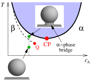
Figure 4: Schematic phase diagram of a binary liquid mixture with a lower demixing transition point in terms of temperature $T$ and concentration $c_{A}$ of the $A$ species. The solid curve encloses the two-phase region separating via first-order phase transitions the $\alpha$ and $\beta$ phases rich in $A$ and $B$ species, respectively, terminating at the critical point CP. The dashed line indicates the first-order bridging phase transition which occurs if a fluid mixture is confined between a planar wall and a sphere of radius $R$ and at distance $L$ possessing the same adsorption preference, here for the $\alpha$ phase. The bridging transition ends at the critical point $Q$ and separates a region in the bulk phase diagram in which a phase preferable by walls condenses and forms a bridge connecting the wall and the sphere, from the region in the bulk phase diagram where such a bridge is absent. Although the bridging transition is a (quasi-) first-order phase transition, in the bulk phase diagram it is described by a line instead of a coexistence region, because it is an interfacial phase transition.

II.2.2 Bridging transition

A bridging transition is the analogue of capillary condensation evans for geometries in which one or both surfaces are non-planar. (However, there is a conceptual difference. Whereas capillary condensation corresponds to an actual shift of the bulk phase diagram, bridging transitions are interfacial phase transitions which leave the bulk phase diagram unchanged but can be described as if effectively the bulk phase boundary of first-order phase transitions is shifted BD ; BBD .) It occurs at temperatures for which two phases may exist, i.e., for $T$ above $T_{c}$ in the case of a binary liquid mixture with a lower consolute point, and it depends on the adsorption properties of the surfaces. If, say, both surfaces favor the $\alpha$ phase rich in species A over the $\beta$ phase rich in species B, one expects the $\alpha$ phase to form a bridge between the surfaces for some chemical potential $\mu_{A}$ of species A such that $\mu_{A}<\mu^{co}_{A}$, where $\mu^{co}_{A}$ is the value corresponding to bulk coexistence. Alternatively, this occurs at a concentration (mole fraction) $c_{A}<c_{A}^{co}$ slightly smaller than its value $c^{co}_{A}$ at bulk coexistence. If the surfaces favor the $\beta$ phase, the $\beta$ phase fills the gap between the surfaces forming a bridge for $\mu_{A}>\mu^{co}_{A}$, i.e., the phase separation line for this morphological transition occurs on the other side of the bulk phase diagram, i.e., for $c_{A}>c^{co}_{A}$ (Fig. 4).

Bridging may occur in the presence of thin wetting layers on both surfaces, i.e., in the partial wetting regimes of the two individual surfaces dobbs ; andrienko ; shinto , or if one or both surfaces are covered by a thick wetting film BBD . Such bridge formation may be relevant for colloid aggregation or flocculation of the particles beysens1 ; beysens2 (for a summary of the corresponding experimental and theoretical work on these phenomena see Refs. BD ; BBD ). For the sphere – planar wall geometry relevant for the present experimental situation, theoretical studies andrienko predict that the bridging transition can occur in the presence of thin wetting layers coating both surfaces. It is a first-order phase transition and ends at a critical point. (Actually, these bridging transitions are only quasi-phase transitions, because they involve, strictly speaking only a zero-dimensional volume BD ; BBD ). For a fixed distance between the wall and the sphere and fixed chemical potential, the position of this critical point is determined by the relation $\xi\simeq R$, where $R$ is the radius of the sphere (see Fig. 4). For small sphere radii the bridge configuration is unstable, even for very small sphere-plane separations. On the other hand, bridging transitions are not possible for large sphere-plane separations, even if the sphere radii are large. The fluid-mediated solvation force between the surfaces is very weak in the absence of the bridge and it is attractive and long-ranged if the capillary bridge is present. Moreover, for $R/\xi$ small its strength is proportional to the sphere-wall separation andrienko ; shinto , contrary to the case of two flat substrates evans or to the sphere-sphere geometry BBD .

II.2.3 Critical Casimir forces for noncritical compositions

For temperatures closer to the critical temperature the solvation force acquires a universal contribution due to the critical fluctuation of the intervening fluid which turns into the critical Casimir force. For a one-component fluid near gas-liquid coexistence $\mu=\mu_{0}(T)$ and confined between parallel plates it has been shown DME that at temperatures near the critical temperature $T_{c}$ a small bulk-like field $h\sim\Delta\mu=\mu-\mu_{0}(T)<0$, which favors the gas phase, leads to residual condensation and consequently to a critical Casimir force which, at the same large wall separation, is much more attractive than the one found exactly at the critical point. The same scenario is expected to apply to binary liquid mixtures, i.e., the Casimir force is expected to be much more attractive for compositions slightly away from the critical composition on that side of the bulk phase diagram which corresponds to the bulk phase disfavored by the confining walls. This has been studied in detail in Ref. colloids1b by using the standard field-theoretic model within mean-field approximation. These studies of the parallel plate geometry have been extended to the case of two spherical particles of radius $R$ at a finite distance $L$ colloids1b . The numerical results for the effective pair potential, as well as the results obtained by using the knowledge of the force between parallel plates and then by applying the Derjaguin approximation, valid for $L\ll R$, show that at $T=T_{c}$ the dependence of the Casimir force on the composition exhibits a pronounced maximum at a noncritical composition. One expects that such a shift of the force maximum to noncritical compositions results from the residual capillary bridging and that the direction of the shift relative to the critical composition depends on the boundary conditions. If the surfaces prefer the $\alpha$ phase rich in species A, by varying the temperature at fixed off-critical composition $c_{A}$, one observes that for small deviations $|c_{A}-c^{c}_{A}|\ll c^{c}_{A}$, the position of the maximum of the Casimir force as function of temperature is almost unchanged, while the absolute value of the maximal force increases considerably by moving away from $c^{c}_{A}$ to compositions $c_{A}<c^{c}_{A}$. The overall temperature variation is, however, similar to that at $c^{c}_{A}$, provided one stays sufficiently close to the critical composition. For compositions $c_{A}$ slightly larger than the critical composition, $c_{A}>c^{c}_{A}$, the critical Casimir force as a function of temperature is expected to behave in a similar way as for $c_{A}<c^{c}_{A}$, but the amplitude of the force maximum should be much weaker and should decrease for increasing $c_{A}$. At compositions further away from $c^{c}_{A}$, i.e., off the critical regime, due to the small bulk correlation length the Casimir force is vanishingly small unless the aforementioned bridging transition is reached by varying the temperature.

The case of a sphere against a planar wall has not been studied theoretically. However, we expect a similar behavior of the effective forces as the one for two spheres.

III Experiment

III.1 The method: Total Internal Reflection Microscopy

III.1.1 Basic principles of TIRM

Total internal reflection microscopy (TIRM) is a technique which allows one to determine the potential $\Phi$ of effective forces acting on a single colloidal particle suspended in a liquid close to a planar substrate, with a force resolution down to the order of femto-Newton. The potential $\Phi$ is obtained from the probability distribution to find the surface of the particle at height $z$ above the substrate, which is determined by monitoring the Brownian motion of the particle in the direction perpendicular to the substrate. In TIRM measurements this is achieved by creating an evanescent light field at the substrate-liquid interface which penetrates into the liquid. The intensity of the evanescent field varies strongly with the distance from the substrate. A single colloidal particle scatters light if it is illuminated by such a field. From this scattered intensity it is possible to deduce the position of the particle in the evanescent field, i.e., to determine $z$ and its time dependence Walz-97 ; Prieve-99 .

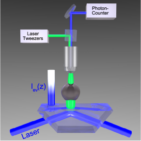
Figure 5: Data acquisition system (see main text for details). The green laser light generated by the optical tweezers is deflected by a double prism into the microscope objective (in the figure represented as a grey vertical cylinder above the spherical particle) and it provides an optical potential which confines the spherical colloid laterally. The blue light which is scattered by this particle out of the evanescent field of intensity $I_{\rm ev}(z)$ is collected by the same microscope objective, focused and then optically directed into the photon counter via a combination of prisms and mirrors (schematically represented in the upper part of the figure).

The basic experimental setup is presented in Fig. 5. A p-polarized laser beam ($\lambda=473$nm, $P=2\,\mbox{mW}$) is directed from below onto the interface between the bottom of a silica glass cell (a cuvette with a chamber to accommodate a fluid film of thickness $200\,\mu\mbox{m}$) and the liquid containing the colloidal particle. The illumination angle $\theta_{i}$ (formed with the substrate normal) is larger than the critical angle $\theta_{c}$ of total internal reflection. Due to total internal reflection, an evanescent wave penetrates into the medium with lower refractive index, here the liquid, and its intensity $I_{\rm ev}(z)$ decays exponentially as a function of the distance $z$ from the glass-liquid interface:

$$I_{\rm ev}(z)=I_{\rm ev}(0){\rm e}^{-\zeta z}\;.$$ (16)

The decay constant $\zeta$ defines the penetration depth $\zeta^{-1}$, which is given by Prieve-99

$$\zeta^{-1}=\frac{\lambda}{4\pi\sqrt{n_{\rm glass}^{2}\sin^{2}\theta_{i}-n_{\rm liq}^{2}}}\,,$$ (17)

where $\lambda$ is the wavelength of the illuminating laser beam in vacuum, and $n_{\rm glass}$ and $n_{\rm liq}$ are the refractive indices of the glass and the liquid, respectively. In our experiment (see, c.f., Sec. III.2) the critical binary mixture (liquid) has $n_{\rm liq}=1.384$ whereas the silica glass (substrate) has $n_{\rm glass}=1.464$ ($>n_{\rm liq}$), resulting in $\theta_{c}\simeq 71^{\circ}$. A colloidal particle with a refractive index $n_{\rm coll}>n_{\rm liq}$ (in our experiment the polystyrene colloids have $n_{\rm coll}=1.59$) at a distance $z$ away from the surface scatters light from the evanescent field. Within the well established data evaluation model for TIRM intensity, the light scattered by the particle has an intensity $I_{\rm sc}$ which is proportional to $I_{\rm sc}\propto I_{\rm ev}(z)$ Prieve-99 and therefore depends on the distance $z$. Care has to be taken in choosing parameters for the penetration depth and the polarization of the illuminating laser beam in order to avoid optical distortions due to multiple reflections between the particle and the substrate, which would spoil the linear relation between $I_{\rm sc}$ and $I_{\rm ev}(z)$. In this respect, safe parameter regions are known to be small penetration depths $\zeta<250$nm and p-polarized illumination as used in the present experiment helden-06 ; hertlein-08 . As a result of this relation, the scattered light intensity $I_{sc}$ exhibits an exponential dependence on the particle-wall distance with exactly the same decay constant $\zeta^{-1}$ ($\zeta^{-1}=200\pm 2\,$nm in our experiment) as the evanescent field intensity $I_{\rm ev}$:

$$I_{\rm sc}(z)=I_{0}\;{\rm e}^{-\zeta z}\,,$$ (18)

where the scattered intensity $I_{0}$ at contact $z=0$ depends on the laser intensity, the combination of refractive indices, and the penetration depth. As will be discussed below, the knowledge of $I_{0}$ is important to determine the particle-substrate distance from the scattered intensity $I_{\rm sc}$. In principle $I_{0}$ could be measured by the so-called sticking method Prieve-99 according to which the particle is stuck on the substrate due to the addition of salt to the liquid in such a way as to suppress the electrostatic stabilization which normally repels the particle from the substrate. However, in the system we are interested in this is not practicable given the large concentration of salt ($>6\,$mM) required to force the particle to stick to the surface and the compact design of the experimental cell which limits the access to the sample. Instead, as described further below, we circumvent this problem by using a hydrodynamic method bevan00 for the absolute determination of the particle-substrate distance.

In Sec. II we mentioned that, upon approaching the critical point of the binary liquid mixture, critical adsorption profiles form near the surfaces of the substrate and of the colloid. These concentration profiles induce a spatial variation of the refractive index, which deviates from the assumed steplike variation underlying Eqs. (16) and (17) (see, e.g., Ref. crit-ads ). Deviations from the functional form given by Eq. (16) are pronounced if the correlation length $\xi$ becomes comparable with the wavelength $\lambda$ of the laser light, which is not the case for the experimental data obtained here, for which $\lambda=473\,$nm and $\xi\lesssim 100\,$nm (see, c.f., Figs. 14, 15, and 16).

In a typical TIRM measurement run, the vertically scattered intensity $I_{\rm sc}(t)=I_{\rm sc}(z(t))$ (photons/s) is recorded by a photomultiplier connected to a single photon counter [see Fig. 5] which counts the total number of scattered photons [see Fig. 6(a)]

$$n_{\rm sc}(t)\equiv\int_{t}^{t+\Delta t}\!\!{\rm d}t^{\prime}I_{\rm sc}(t^{\prime})\simeq I_{\rm sc}(t)\Delta t$$ (19)

detected within a time interval $\Delta t=1\,$ms footnote_nvsI . The value of $n_{\rm sc}(t)$ is then acquired with a frequency $f_{\rm samp}=250\,$Hz for a total duration $t_{\rm samp}\simeq 15\,$min. The resulting set of data is then analyzed as described below in Sec. III.1.2. Consecutive intensity data $I_{\rm sc}(t)$, i.e., $n_{\rm sc}(t)$ acquired with a larger frequency $f_{\rm samp}$ turn out to be strongly correlated in time. Accordingly, their acquisition does not contribute to the reduction of the statistical errors affecting the final estimate for the potential, as will be discussed in, c.f., Sec. IV.2.2. This observation motivates our choice $f_{\rm samp}=250\,$Hz.

In addition to the detection optics, an optical tweezer is implemented in the TIRM setup ash-70 in order to be able to control the lateral position of the particle. The tweezer is created by a laser beam ($\lambda_{\rm tweezer}=532\,$nm) incident on the particle from the direction perpendicular to the substrate and focused by the microscope objective used also for the detection (see Fig. 5). Via this tweezer it is possible to conveniently position the probe particle within the measuring cell and to restrict its lateral diffusion to a few microns so that the particle does not diffuse out of the field of view of the detection system. In addition, the tweezer also exerts a light pressure walz92 onto the particle, increasing significantly its effective weight (in the specific case considered here from ca. $1.1k_{\mathrm{B}}T_{c}/\mu\mbox{m}$ to ca. $7k_{\mathrm{B}}T_{c}/\mu\mbox{m}$, see, c.f., Sec. III.1.3 and Refs. footnoteB ; dataWL for details). In our experiment the tweezer is typically operated at a low power of $P\simeq 2\,$mW, but even at the largest power ($P_{\rm max}\simeq 25\,$mW) we used to trap and move the particle no effects of local heating, such as the onset of phase separation in the liquid, were observed due to the laser of the tweezer.

III.1.2 Data analysis

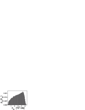
(a)	(b)	(c)

Figure 6: Data analysis: (a) Raw data for the total number of scattered photons $n_{\rm sc}(t)$ detected at a certain time $t$ within a time interval $\Delta t=1\,\mbox{ms}$ from the single photon counter as a function of time, taken for a sampling time $t_{\rm samp}\simeq 15\,$min. (b) Histogram calculated from this time series yielding the distribution function $p_{\rm sc}(n_{\rm sc})$ of the number $n_{\rm sc}$ of scattered photons. (c) The knowledge of the relation [see Eq. (18)] between the scattered intensity $I_{\rm sc}\simeq n_{\rm sc}/\Delta t$ and the position $z$ of the colloid in the evanescent field allows one to determine the probability distribution $p_{z}(z)=\zeta n_{\rm sc}(z)p_{\rm sc}(n_{\rm sc}(z))$ for the particle-substrate distance $z$ from $p_{\rm sc}(n_{\rm sc})$ and therewith by inversion of the Boltzmann factor the interaction potential. Further details are given in the main text.

In order to determine the potential $\Phi$ of the effective forces acting on the colloidal particle, one constructs a histogram out of the values of $n_{\rm sc}(t)$ [see Eq. (19)] recorded in the time interval $t_{\rm samp}$, in such a way as to determine the probability distribution function $p_{\rm sc}(n_{\rm sc})$ for the particle to scatter $n_{\rm sc}=I_{\rm sc}\Delta t$ photons in a time interval $\Delta t$. Within the sampling time $t_{\rm samp}$ there are $t_{\rm samp}f_{\rm samp}=N$ registration of counts. If $N^{*}$ is the number of registrations which yield a certain count $n_{\rm sc}^{*}$, the probability $p(n_{\rm sc}^{*})$ of $n_{\rm sc}^{*}$ to occur is $N^{*}/N$. By using $p_{\rm sc}(n_{\rm sc}){\rm d}n_{\rm sc}=p_{z}(z){\rm d}z$ and Eq. (18), this probability distribution $p_{\rm sc}(n_{\rm sc})$ can be transformed into the probability

$$p_{z}(z)=\zeta\,n_{\rm sc}(z)\,p_{\rm sc}(n_{\rm sc}(z))$$ (20)

for the particle-substrate distance $z$. In turn, in thermal equilibrium at temperature $T$, the probability $p_{z}(z)$ is related to the particle-wall interaction potential $\Phi(z)$ by the Boltzmann factor

$$p_{z}(z)=C\exp\left[-\Phi(z)/(k_{\mathrm{B}}T)\right],$$ (21)

where $k_{B}T$ is the thermal energy and $C$ a normalization constant. Equation (21) holds because, due to the high dilution of the colloidal suspension, the single colloidal particle under observation does not interact with other particles. As a result, from the knowledge of $p_{\rm sc}(n_{\rm sc})$ it is possible to determine $\Phi(z)$ up to an irrelevant constant related to $C$ and to the overall normalization of $p_{\rm sc}(n_{\rm sc})$. For each bin of the histogram of $p_{\rm sc}(n_{\rm sc})$, the corresponding distance $z(n_{\rm sc})$ is calculated via inversion of Eq. (18):

$$z(n_{\rm sc})=-\zeta^{-1}\ln[n_{\rm sc}/(I_{0}\Delta t)]=z_{\rm exp}(n_{\rm sc})-z_{0}$$ (22)

where $z_{\rm exp}(n_{\rm sc})=-\zeta^{-1}\ln n_{\rm sc}$ is given in terms of experimentally accessible quantities (i.e., $n_{\rm sc}$ and $\zeta$). This provides the position of the particle up to the constant $z_{0}=-\zeta^{-1}\ln(I_{0}\Delta t)$ as the experimentally yet unknown position of the wall footnote1 [$I_{\rm sc}(z=0)=I_{0}$]. In order to determine $z_{0}$ for all data sets, we have employed the so-called hydrodynamic method bevan00 , which is based on the fact that due to hydrodynamic interactions the diffusion coefficient $D$ of a colloidal particle at a distance $z$ from the wall strongly depends on $z$. Moreover, near a wall the diffusion coefficient becomes also spatially anisotropic with the relevant value for TIRM measurements being $D_{\bot}$, which refers to the diffusion occurring in the direction perpendicular to the wall. Its spatial dependence can be expressed as

$$D_{\bot}=D_{\infty}f(z/R)$$ (23)

where $D_{\infty}=k_{\mathrm{B}}T/(6\pi\eta R)$ is the bulk diffusion coefficient of a spherical particle of radius $R$ in a homogeneous fluid with viscosity $\eta$ at temperature $T$. (For the water-lutidine mixture we use in our experiments, the value of $\eta$ has been measured in Ref. clu99 as a function of temperature $T$ and composition, with $\eta\simeq 2.09\times 10^{-3}$Pa s at $T=31^{\circ}$C and at the critical composition.) The reduced mobility function $f(v)$ was calculated in Ref. gold67 and can be well approximated by bevan00 :

$$f(v)=\frac{6v^{2}+2v}{6v^{2}+9v+2}\,.$$ (24)

A plot of this theoretically predicted distance-dependent diffusion coefficient $D_{\bot}$ is shown in Fig. 7.

Figure 7: Diffusion coefficient $D_{\bot}$ of a spherical particle of radius $R$ moving perpendicular to a wall at a distance $z$ gold67 ; bevan00 . $D_{\infty}$ is the bulk diffusion coefficient. Note that for the present experimental conditions $z/R<1$ and thus this distance dependence is pronounced.

A well established method bevan00 to determine the absolute particle-wall distance is to calculate the apparent diffusion coefficient $D_{\rm app}$ which is the weighted average of $D_{\bot}(z)$ over the distances sampled by the colloidal particle, i.e., $D_{\rm app}=\int_{0}^{\infty}{\rm d}z\,D_{\bot}(z){\rm e}^{-2\zeta z}p_{z}(z)/\int_{0}^{\infty}{\rm d}z\,{\rm e}^{-2\zeta z}p_{z}(z)$, where the exponential factors in the numerator and denominator reflect the spatial dependence of $I^{2}_{\rm sc}(z)$ [see Eq. (18) and below]. This apparent diffusion coefficient can be experimentally determined from the initial slope of the autocorrelation function $C(\delta t)=\langle n_{\rm sc}(t)n_{\rm sc}(t+\delta t)\rangle_{t}$ of the scattering intensity bevan00 :

$$D_{\rm app}=-\frac{1}{\zeta^{2}}\frac{C^{\prime}(0)}{C(0)}$$ (25)

where the prime ^′ denotes the derivative with respect to $\delta t$. In order to determine $z_{0}$ one calculates the apparent diffusion coefficient $D_{\rm app,calc}$ on the basis of $D_{\bot}(z)$ and of the experimentally determined probability distribution $p_{z}$ which is given by the parametric plot of $\zeta n_{\rm sc}p_{\rm sc}(n_{\rm sc})$ as a function of $z_{\rm exp}(n_{\rm sc})-\hat{z}_{0}$ upon varying $n_{\rm sc}$ [Eqs. (20) and (22)], with $\hat{z}_{0}$ as the yet unknown position of the wall, and according to which the colloidal particle samples distances. In turn, the value $\hat{z}_{0}=z_{0}$ can be determined by requiring that $D_{\rm app}=D_{\rm app,calc}$. A detailed description of this procedure can be found in Ref. bevan00 . The uncertainty in the determination of $z_{0}$ via this method (see Appendix B of Ref. bevan00 ) is primarily determined by the uncertainties of the particle radius [see Eqs. (23) and (24)] and of the penetration depth $\zeta^{-1}$ [see Eq. (25)]. Considering the experimental parameters and errors of our measurements, the resulting uncertainty in the particle-substrate distance $z$ can be estimated to be $\pm 30\,$nm for all plots shown in the following.

We emphasize that it is sufficient to determine $z_{0}$ at a certain temperature in order to fix it for all the measured potential curves at different temperatures. Indeed the intensity $I_{\rm ev}(0)$ of the evanescent field at the glass-liquid surface [as well as $\zeta^{-1}$, see Eq.(17)] depends on temperature via the temperature dependence of the optical properties of the glass and the liquid. In turn, this would imply a variation of the critical angle $\theta_{c}$ with $T$, which was actually not observed within the range of temperatures investigated here. The intensity $I_{0}\propto I_{\rm ev}(0)$, which determines $z_{0}$ and which is recorded by the photomultiplier, is in principle affected by the temperature-dependent background light scattering due to the critical fluctuations within the mixture (critical opalescence). For the typical intensities involved in our experiment and for the temperature range studied, the contribution of this background scattering is actually negligible and, as a result, $z_{0}$ does not change significantly with temperature. The hydrodynamic method, however, requires the knowledge of the viscosity $\eta$ of the mixture, which depends on temperature and sharply increases upon approaching the critical point clu99 due to critical fluctuations. These fluctuations might in addition modify the expression of $D_{\perp}(z)$. In order to reduce this influence of critical fluctuations we have chosen $T_{c}-3\,$K as the reference temperature for determining $z_{0}$, corresponding to a temperature at which no critical Casimir forces could actually be detected in the interaction potential.

III.1.3 Interaction potentials

Under the influence of gravity, buoyancy, and the radiation field of the optical tweezer as external forces, the total potential $\Phi$ of the colloidal particle floating in the binary liquid mixture, as determined via TIRM, is the sum of four contributions:

$$\Phi(z)=\Phi_{0}(z)+G_{\rm eff}z+\Phi_{C}(z)+\Phi_{\rm offset}\,.$$ (26)

In this expression $\Phi_{0}$ is the potential due to the electrostatic interaction between the colloid and the wall and due to dispersion forces acting on the colloid; it is typically characterized by a short-ranged repulsion and a long-ranged attraction. The combined action of gravity, buoyancy, and light pressure from the optical tweezer is responsible for the linear term $G_{\rm eff}z$ in Eq. (26) (see, e.g., Ref. walz92 ). $\Phi_{C}(z)$ is the critical Casimir potential arising from the critical fluctuations in the binary mixture. The last term $\Phi_{\rm offset}$ is an undetermined, spatially constant offset different for each measured potential which accounts for the potentially different normalization constants of the distribution functions $p_{I}$ and $p_{z}$. While the first two contributions are expected to depend mildly on the temperature $T$ of the fluid, the third one should bear a clear signature of the approach to the critical point. These expectations are supported by the experimental findings reported in Sec. IV. The typical values of $G_{\rm eff}$ for the measurements presented in Sec. IV are $G_{\rm eff}\simeq 7.2k_{B}T/\mu$m and $G_{\rm eff}\simeq 10.0k_{B}T/\mu$m for the colloids with diameters $2R=2.4\mu$m and $3.68\mu$m, respectively footnoteB . Far enough from the surface, $\Phi_{0}$ and $\Phi_{C}$ are negligible compared to the linear term and therefore the typical potential $\Phi(z)$ is characterized by a linear increase for $z$ large enough. Accordingly, upon comparing potentials determined experimentally at different temperatures, the corresponding additive constants $\Phi_{\rm offset}$, which are left undetermined by the TIRM method, can be fixed consistently such that the linearly increasing parts of the various $\Phi$ coincide. However, it may happen that at some temperatures the total potential $\Phi$ develops such a deep potential minimum that the colloid cannot escape from it and therefore the gravitational tail is not sampled. If this occurs the shift of this potential by a constant cannot be fixed by comparison with the potentials measured at different temperatures. In order to highlight the interesting contributions to the potentials, the term $G_{\rm eff}z$, common to all of them, is subtracted within each series of measurements and for all boundary conditions. Accordingly, the remaining part of the potential — displayed in the figures below — decays to zero at large distances.

On the other hand, closer to the substrate, the (non-retarded) van-der-Waals forces contribute to $\Phi_{0}(z)$ with a term (see, e.g., Ref. vdW , Tab. S.5.b)

$$\Phi_{0,{\rm vdW}}(z)=-\frac{A}{6}\left[\frac{1}{\delta}+\frac{1}{2+\delta}-\ln(1+2/\delta)\right],$$ (27)

where $A$ is the Hamaker constant and $\delta=z/R$. As $\delta$ increases, this term crosses over from the behavior $\Phi_{0,{\rm vdW}}(z\ll R)\simeq-(A/6)(R/z)$ to $\Phi_{0,{\rm vdW}}(z\gg R)\simeq-(2A/9)(R/z)^{3}$. The dependence of $\Phi_{0,{\rm vdW}}(z\ll R)$ on $z$ is the same as the one of $\Phi_{C}(z\ll\xi,R)$ (see Eq. (12)) and therefore their relative magnitude is controlled by $|\Phi_{0,{\rm vdW}}(z\ll R)/\Phi_{C}(z\ll\xi,R)|=[A/(k_{\mathrm{B}}T)]1/[6\Theta(0)]\simeq 2.4/(6\Theta(0))$ for a critical point at $T\simeq 300$ K and a typical value of the Hamaker constant $A\simeq 10^{-20}$ J. Taking into account that $\Theta_{{(+,+)}}(0)\simeq 2.5$ and $\Theta_{{(+,-)}}(0)\simeq 15$ it is clear that in this range of distances the critical Casimir potential typically dominates the (non-retarded) van-der-Waals interaction. Note, however, that for small values of $z$ both of them become negligible compared to the electrostatic repulsion. For larger values of $R\ll z\ll\xi$, the Casimir force still dominates the dispersion forces, as discussed in detail in Refs. colloids1a ; colloids1b . However, for the present experimental conditions, the distance $z$ is comparable to the bulk correlation length $\xi$ and actually most of the data refer to the case $\xi\lesssim z\lesssim R$, with the values of the scaling variables ranging between $z/\xi\simeq 10$ and $z/R\simeq 0.6$ for distances at which the corresponding potential is still experimentally detectable. Accordingly, with the above estimate for the potential ratio, one can conservatively estimate $|\Phi_{0,{\rm vdW}}(z\sim 0.6R)/\Phi_{C}(z\sim 10\xi)|=[A/(k_{\mathrm{B}}T)](0.2/|\Theta(10)|)\simeq 0.2$ where $\Theta_{{(+,-)}}(10)\simeq-\Theta_{{(+,+)}}(10)\simeq 2.5$. Retardation causes the van-der-Waals potential to decay as a function of $z$ more rapidly than predicted by Eq. (27). This additionally reduces the contribution of $\Phi_{0,{\rm vdW}}$ compared with $\Phi_{C}$. In the analysis of the experimental data in Sec. IV we shall reconsider the Hamaker constant $A$ for the specific system we are dealing with.

In order to achieve the accuracy of the temperature control needed for our measurements we have designed a cell-holder rendering a temperature stability of $\pm 5\,$mK. This has been accomplished by using a flow thermostat coupled to the cell holder with a temperature of $(30.50\pm 0.01)^{\circ}$C functioning as a heat sink and shield against temperature fluctuations of the environment. In order to fine tune the temperature the cell was placed on a transparent ITO (indium-tin-oxide) coated glass plate for a homogeneous heating of the sample from below. The voltage applied to the ITO coating was controlled via an Eurotherm proportional-integral-derivative (PID) controller for approaching the demixing temperature. The controller feedback provides a temperature stability of $\pm 2\,$mK at the position of the Pt$100$-sensor used for temperature measurements. However, since the probe particle is displaced from the sensor by a few millimeter, some additional fluctuations have to be considered. From the reproducibility of the potential measurements and from the relative temperature fluctuations of two independent Pt100 sensors placed on either side of the cell we inferred a $\pm 5\,$mK stability of the temperature at the actual position of the measurement. The highly temperature sensitive measurements were affected neither by the illuminating nor by the tweezing lasers due to moderate laser powers and due to low absorption by the probe particle and by the surface. Although all measurements were carried out upon approaching the demixing temperature, the light which is increasingly scattered in the bulk background by the correlated fluctuations of the binary liquid mixture exposed to the evanescent field turned out to be negligible compared to the light scattered directly by the colloid. The effects of the onset of critical opalescence are significantly reduced by the fact that the illuminating optical field rapidly vanishes upon increasing the distance from the substrate and due to the still relatively small values of the correlation length.

III.2 The binary liquid mixture and boundary conditions

For providing the critical fluctuations we have chosen the binary liquid mixture of water and $2,6$-lutidine near its demixing phase transition. The bulk phase diagram of such a binary liquid mixture prepared at room temperature, ambient pressure, and sealed in a cell WL-phdiag (constant volume) is reported in Fig. 8(a). It is characterized by a one-phase region (disordered phase) in which the two components form a mixed solution and which surrounds the closed loop of the two-phase region (ordered phase) in which these components segregate into a water-rich and a lutidine-rich phase. The first-order transition line delimiting the two-phase coexistence region, within which the two ordered phases form an interface, ends in a lower critical demixing point (LCP, see Fig. 8(a)) at the lutidine mass fraction $c^{c}_{L}\simeq 0.28$ and the critical temperature $T_{c}\simeq 307.15\,$K beysens1 . The upper critical demixing point (UCP, see Fig. 8(a)) is located at high temperatures and therefore it occurs within the liquid phase only at pressure values above ambient ones.

The choice of this specific binary liquid mixture as the critical medium is motivated by the fact that its properties (bulk phase diagram, refractive index, viscosity, etc.) are known rather well and are documented in the literature, as this mixture has been extensively employed in the past for the study of phase separation per se or as a solvent of colloidal dispersions. A clear experimental advantage is provided by the fact that the water-lutidine mixture at ambient pressure has a lower critical point slightly above room temperature which can be conveniently accessed from the one-phase region by heating the sample. Alternative binary liquid mixtures with a lower demixing point close to room temperature are formed by water and, e.g., 2,5-lutidine ($T_{c}\simeq 13^{\circ}$), 2,4-lutidine ($T_{c}\simeq 23^{\circ}$C), triethylamine ($T_{c}\simeq 18^{\circ}$C), and $n$-butoxyethanol ($T_{c}\simeq 49^{\circ}$C). The addition of a suitable amount of a third component to some of these binary liquid mixtures allows one to shift the critical temperature of demixing basically at will. For example, by adding 3-methylpyridine to the presently used mixture of 2,6-lutine and water it is possible to gradually shrink the coexistence loop in Fig. 8(a), causing an upwards shift of $T_{c}$ of as much as $30^{\circ}$C. Analogously, even though 3-methylpyridine is always miscible with normal water, it exhibits a coexistence loop if mixed with heavy water, with a lower critical point at $T_{c}\simeq 39^{\circ}$C. The addition of normal water to this demixing binary liquid mixture of heavy water and 3-methylpyridine causes an upwards shift of $T_{c}$ until the coexistence loop disappears at a double critical point with $T_{c}^{\rm dcp}=78^{\circ}$C WL-phdiag . The variety of available substances and the tunability of the critical temperature by suitable chemical additions allow one to generate critical Casimir forces for a conveniently wide range of temperatures.

In our experiment the mixture is prepared under normal conditions (room temperature, ambient pressure) and then it is introduced into the sample cell which is afterwards sealed with Teflon plugs in order to hinder the mixture from evaporating. Although we have no control on the resulting pressure $p$ of the mixture, the fact that the cell is not hermetically sealed and that small air bubbles might be trapped within it should keep $p$ very close to its ambient value. Within the limited range of temperatures we shall explore in the experiment, possible pressure variations are not expected to lead to substantial modifications of the phase diagram (e.g., shifts of the critical point) compared to the ones at constant pressure or volume.

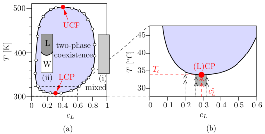
Figure 8: Bulk phase diagram of the binary liquid mixture of water and 2,6-lutidine (dimethylpyridine ${\rm C}_{7}{\rm H}_{9}{\rm N}$) WL-phdiag ; beysens1 at constant volume. The relevant thermodynamic variables are the temperature $T$ and the mass fraction $c_{L}$ of lutidine in the mixture. Open symbols in panel (a) refer to actual experimental data WL-phdiag . The schematic side view of a vertical sealed cell filled with the binary liquid mixture is shown by the insets (i) and (ii) of panel (a) for thermodynamic states outside and inside of the coexistence loop, respectively. In (ii) W and L indicate the water- and the lutidine-rich phase, respectively. The mixture separates into the lutidine-rich and the water-rich phase within the two-phase coexistence area encircled by the solid first-order transition line. At the lowest and highest points (LCP and UCP, respectively) of this line the demixing transition is continuous. The detailed phase diagram in the vicinity of the lower critical point is shown in panel (b), together with the typical thermodynamic paths (dashed vertical lines) experimentally investigated here within the gray region as well as for $c_{L}=0.2$.

The order parameter $\phi$ for the demixing phase transition can be taken to be the difference between the local concentration $c_{L}({\bf x})$ (mass fraction) of lutidine in the mixture and its spatially averaged value $c_{L}$. Accordingly, a surface which preferentially adsorbs lutidine is referred to as realizing the $(+)$ boundary condition for the order parameter given that it favors $\phi>0$, whereas a surface which preferentially adsorbs water leads to the $(-)$ boundary condition.

The experimental cell containing the binary liquid mixture and the colloid is made up of silica glass. Depending on the chemical treatment of its internal surface, one can change the adsorption properties of the substrate so that it exhibits a clear preference for either one of the two components of the binary mixture. In particular, treating the surface with NaOH leads to preferential adsorption of water $(-)$, whereas a treatment with hexamethyldisilazane (HMDS) favors the adsorption of lutidine $(+)$ footnote_det_exp , as we have experimentally verified by comparing the resulting contact angles for water and lutidine on these substrates. As colloids we used polystyrene particles of nominal diameter $2R=3.69\,\mu$m and $2.4\mu$m, the latter possessing a rather high nominal surface charge density of 10$\mu$C/cm². Size polydispersity of these particles are $2\%$ and $3\%$, respectively, corresponding to ca. $\pm 70\,$nm. (These nominal values are provided in the data-sheets of the company producing the batch of particles, see Ref. nature for details.) The adsorption properties of polystyrene particles in a water-lutidine mixture have been investigated in Refs. gm-92 ; gkm-92 , with the result that highly charged ($\gtrsim 3.8\mu$C/cm²) colloids preferentially adsorb water (highly polar) whereas lutidine is preferred at lower surface charges. Even though we did not independently determine these adsorption properties, the results of Refs. gm-92 ; gkm-92 and the corresponding nominal values of the surface charges of the colloids employed in our experiment suggest that the polystyrene particles of diameter $2R=3.69\,\mu$m [$2R=2.4\,\mu$m] have a clear preference for lutidine $(+)$ [water $(-)$]. A posteriori, these presumed preferential adsorptions are consistent with the resulting sign of the critical Casimir force observed experimentally. Depending on the surface treatment of the cell and the choice of the colloid one can realize easily all possible combinations of (particle, substrate) boundary conditions (see Tab. 1).

(particle, substr.)	colloid diam. $2R$:
substrate treat.:	ai3.69$\mu$mai	ai2.4$\mu$mai
HMDS	${(+,+)}$	${(-,+)}$
NaOH	${(+,-)}$	${(-,-)}$

Table 1: Experimental realization of all possible (particle, substrate) symmetry-breaking boundary conditions, where $(+)$ indicates the preferential adsorption of lutidine and $(-)$ the preferential adsorption of water. The treatments of the substrate affect only its surface properties.

For a given choice of the particle-substrate combination with its boundary conditions and for a given concentration $c_{L}$ of the mixture we have determined the interaction potential $\Phi$ (see Eq. (26)) between the colloid and the substrate as described in the previous subsection, starting from a temperature $T$ below the critical point in the one-phase region and then increasing it towards that of the demixing phase transition line at this value of $c_{L}$. It might happen that, as a result of leaching, the water-lutidine mixture slowly (i.e., within several days) alters the surface properties of the colloidal particles we used in the experiment. In order to rule out a possible degradation of the colloid during the experiment, we verified the reproducibility of the observed effects after each data acquisition.

IV Results

In, c.f., Figs. 10–13 and 17 we report the experimentally obtained interaction potentials $\Phi$ as functions of the particle-wall distance $z$ for various values of the temperature $T$, both at critical (Figs. 10–13) and off-critical concentrations (Fig. 17). In all the cases presented, the gravitational and offset parts of the potentials [see Eq. (26)], which turn out to be de facto independent of the temperature $T$, have been subtracted in such a way that the resulting potentials vanish for large values of $z$. However, those potentials, for which the gravitational tail could not be sampled (see, e.g., Figs. 12 and 17), cannot be normalized like the others by this requirement.

Depending on the concentration of the mixture, two qualitatively different behaviors are observed, which are discussed in Sec. IV.2 for $c_{L}=c_{L}^{c}$ and in Sec. IV.3 for $c_{L}\neq c_{L}^{c}$. However, in the next subsection we first discuss the experimental results for the potentials measured far away from the transition line and the comparison of them with theoretical predictions. This provides important insight into the effective background forces to which the critical Casimir forces add upon approaching the critical point.

IV.1 Non-critical potentials

In all the cases reported here, sufficiently far from the transition line one observes a potential which appears to consist only of the electrostatic repulsion between the colloid and the substrate and which can be fitted well by

$$\Phi_{0}(z)=k_{\mathrm{B}}T\,{\rm e}^{-\kappa(z-z_{\rm es})}$$ (28)

where $\kappa^{-1}$ is the Debye screening length and $z_{\rm es}$ the value of the distance $z$ at which $\Phi_{0}(z=z_{\rm es})=k_{\mathrm{B}}T$. ($z_{\rm es}$ is expected to depend, inter alia, on the surface charge and on the radius of the colloid.) For the potential in, c.f., Fig. 10 which corresponds to $T_{c}-T=300\,\mbox{mK}$, a fit of $\kappa$ yields $\kappa^{-1}=12\mbox{nm}\pm 3\mbox{nm}$, which is compatible with the estimate $\kappa^{-1}\simeq 10\,$nm derived from the standard expression $\kappa=\sqrt{e^{2}\sum_{i}\rho_{i}/(\varepsilon_{\rm liq}(0)k_{\mathrm{B}}T)}$ (see, e.g., Ref. vdW ), where $e$ is the elementary charge, $\varepsilon_{\rm liq}(0)$ the static permittivity of the mixture (see below), and $\rho_{i}$ the number density of ions assumed to be monovalent and estimated in Ref. gm-92 for the dissociation of a salt-free water-lutidine mixture. Within the range of distances $z$ sampled in our experiment there is no indication of the presence of an attractive tail in $\Phi_{0}$, which on the other hand is generically expected to occur due to dispersion forces, described by a potential as given in Eq. (27). In order to compare this experimental evidence with theoretical predictions, below we shall discuss the determination of the Hamaker constant $A$ in Eq. (27) on the basis of the dielectric properties of the materials involved in the experiment. The relation between them is provided by (see, e.g., Ref. vdW )

$$\begin{split}A(z)&\simeq\frac{3}{2}k_{\mathrm{B}}T\sum_{n=0}^{\infty}\!{}^{\prime}\,\,\left.\frac{\varepsilon_{\rm glass}-\varepsilon_{\rm liq}}{\varepsilon_{\rm glass}+\varepsilon_{\rm liq}}\,\frac{\varepsilon_{\rm coll}-\varepsilon_{\rm liq}}{\varepsilon_{\rm coll}+\varepsilon_{\rm liq}}\,\right|_{i\omega_{n}}\!\!R_{n}(z)\\ &\equiv A_{n=0}+A_{n>0}\end{split}$$ (29)

where the permittivities $\varepsilon$ of the various materials are evaluated at the imaginary frequencies $i\omega_{n}$, with $\omega_{n}=2\pi k_{\mathrm{B}}Tn/\hbar=n\times 2.5\times 10^{14}\,$rad/s at $T\simeq 300\,$K. (Note that the imaginary part of the complex permittivity $\varepsilon(\omega)$ as a function of the complex frequency $\omega$ vanishes on the imaginary axis $\mbox{Re\,}\omega=0$ vdW .) The factor $R_{n}(z)$ accounts for retardation and, neglecting the fact that in the three different media light propagates with different velocities (i.e., for $R_{n}$ assuming $\varepsilon_{\rm coll}\simeq\varepsilon_{\rm liq}\simeq\varepsilon_{\rm coll}$) it takes the form $R_{n}=(1+r_{n}){\rm e}^{-r_{n}}$. The ratio $r_{n}\equiv 2\tau_{n}(z)/\omega_{n}^{-1}$ quantifies the relevance of retardation: heuristically, a thermally fluctuating electric dipole within, e.g., the glass generates an electric field which travels at least a distance $z$ across the liquid, taking a minimal time $\tau_{n}(z)=z/(c/\sqrt{\varepsilon_{\rm liq}(i\omega_{n})})$, before inducing an electric dipole within the colloid. Such an induced dipole, in turn, generates an electric field which travels back to the original dipole and interacts with it. However, such an interaction is reduced by the fact that the original dipole has a lifetime $\omega_{n}^{-1}$ and might have decayed during the minimal time $2\tau_{n}(z)$ it takes the electric field to do the roundtrip vdW , which is the case for $r_{n}\equiv 2\tau_{n}(z)/\omega_{n}^{-1}\gtrsim 1$. The prime in Eq. (29) indicates that the contribution of the static permittivities $n=0$ is to be multiplied by $1/2$ (see, e.g., Ref. vdW ), resulting in the term $A_{n=0}$. Within a first approximation, in Eq. (29) the retardation factor $R_{n}$ does not affect those terms with $r_{n}\lesssim 1$, corresponding to $R_{n}\simeq 1$ for them, while it exponentially suppresses those terms with $r_{n}\gg 1$. Accordingly, only the former contribute significantly to $A_{n>0}$ and retardation is accounted for by summing in $A_{n>0}$ only the terms corresponding to $\omega_{n}\lesssim(c/\sqrt{\varepsilon(i\omega_{n})})/(2z)$, where $\sqrt{\varepsilon(i\omega_{n})}\simeq n_{\rm liq}$ (see, c.f., dash-dotted line in Fig. 9 for $n=1,\ldots,4$) is the refractive index of the liquid. The expression in Eq. (29) is valid generically for a film and only in the non-retarded regime $R_{n}\simeq 1$ for the sphere-plate geometry. However, even for the latter geometry an estimate of the order of magnitude of the effects of retardation can be inferred simply by restricting the sum in Eq. (29) to the values of $n$ corresponding to $r_{n}\lesssim 1$, so that $R_{n}\simeq 1$.

The parameters of our experiment, i.e., $z\gtrsim 0.1\,\mu$m and $n_{\rm liq}\simeq 1.38$ yield $\omega_{n}\lesssim 1.1\times 10^{15}$ Hz, i.e., $n\leq 4$ at $T\simeq 300\,$K, with $\omega_{n=1,\ldots,4}$ in the infrared (IR) spectrum. The contribution $A_{n=0}$ of the zero-frequency mode is actually subject to screening by the salt in the liquid solution, characterized by the Debye screening length $\kappa^{-1}$ which also controls the exponential decay of the electrostatic contribution to $\Phi_{0}$. This means that $A_{n=0}$ is not a constant but acquires a $z$ dependence. This is accounted for by a multiplicative correction factor $R_{0}(z)=(1+2\kappa z){\rm e}^{-2\kappa z}$ multiplying $A_{n=0}$ as given by Eq. (29); we note that $R_{0}(0)=1\geq R_{0}(z)$. A parametric representation of the permittivity $\varepsilon_{\rm W}(i\omega)$ of pure water can be found in Table L2.1 in Ref. vdW . In the part of the spectrum over which the sum in Eq. (29) runs, for polystyrene the permittivity $\varepsilon_{\rm coll}(i\omega)$ is actually almost constant $\varepsilon_{\rm coll}=n_{\rm coll}^{2}\simeq 2.53$ (see, e.g., Table L2.3 in Ref. vdW for a parameterization). For lutidine and silica, the parameters which characterize the corresponding permittivities $\varepsilon_{\rm L}(i\omega)$ and $\varepsilon_{\rm glass}(i\omega)$ are summarized in Table 1 of Ref. PLB-98 . In order to calculate the dielectric permittivity $\varepsilon_{\rm liq}(i\omega)$ of the homogeneous water-lutidine mixture on the basis of $\varepsilon_{\rm W}$, $\varepsilon_{\rm L}$, and the lutidine volume fraction $\phi_{\rm L}\simeq 0.25$, one can use the Clausius-Mossotti relation, as explained in Ref. PLB-98 . The resulting permittivities are reported in Fig. 9.

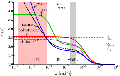
Figure 9: Permittivities $\varepsilon(i\omega)$ of the materials relevant for our experiment as functions of the frequency $\omega$ [rad/s] on a logarithmic scale. As on the left, from bottom to top, we report the curves corresponding to pure lutidine, polystyrene ($\varepsilon_{\rm coll}$), silica ($\varepsilon_{\rm glass}$), a water-lutidine mixture with a volume concentration $\phi_{\rm L}\simeq 0.25$ of lutidine ($\varepsilon_{\rm liq}$), and pure water. These curves are based on the parameterizations and on the material properties reported in Refs. vdW ; PLB-98 . The four vertical lines indicate the frequencies $\{\omega_{n}\}_{n=1,\ldots 4}$ which within our approximation enter into the determination of the Hamaker constant in Eq. (29). (Note that $\mbox{Im\,}\varepsilon(\omega)=0$ if, as in the present case, $\mbox{Re\,}\omega=0$ vdW .)

With these elements at hand and within the approximation discussed above one can calculate an upper bound to the value of $A_{n>0}$ which accounts for retardation, finding

$$A_{n>0}(z\gtrsim 0.1\,\mu\mbox{m})\lesssim 0.06\,k_{\mathrm{B}}T\simeq 0.025\times 10^{-20}{\rm J}.$$ (30)

In addition, from Eq. (29) and from the material parameters one finds

$$A_{n=0}\simeq 0.46\,k_{\mathrm{B}}T$$ (31)

resulting in a screened contribution $A_{n=0}^{\rm(scr)}(z)=A_{n=0}R_{0}(z)$, with $\kappa^{-1}\simeq 12$nm, which is actually negligible compared to the electrostatic potential $\Phi_{0}$ [see Eq. (28)]: $A_{n=0}^{\rm(scr)}(z)/\Phi_{0}(z)\lesssim A_{n=0}{\rm e}^{-\kappa z_{\rm es}}\lesssim 6\times 10^{-4}$ (c.f., Tab. 2 for typical values of $\kappa$ and $z_{\rm es}$). Taking into account Eq. (27), the contribution of $A_{n=0}^{\rm(scr)}$ to $\Phi_{0,{\rm vdW}}(z)$ becomes comparable to the electrostatic one only for $z/R\lesssim 10^{-4}$, which is well below the range $z/R\gtrsim 0.1$ actually investigated in our experiment. On the other hand, for $z\simeq 0.1\,\mu$m, $A_{n=0}^{\rm(scr)}\simeq 0.004\,k_{\mathrm{B}}T$ and due to its exponential decay with $z$, we expect this contribution to be negligible compared to the value $A_{n>0}(z\gtrsim 0.1\,\mu\mbox{m})$ in Eq. (30). In turn, this value is considerably smaller than the typical one $A\simeq 10^{-20}$J we have used in Sec. III.1.3 in order to compare dispersion forces with the critical Casimir potential. Accordingly, the conclusion drawn there that the latter typically dominates the former is confirmed and reinforced by the estimate for $A$ given here.

The values just determined for $A_{n=0}$ and $A_{n>0}$ are meant to be estimates of their orders of magnitude given that a detailed calculation which properly accounts for retardation (following, e.g., Ref. PLB-98 ) and for possible inhomogeneities in the media, especially within a binary liquid mixture, goes beyond the present scope of a qualitative comparison of theoretical predictions for the background forces with the actual experimental data. In this respect, a detailed determination of the permittivities of the specific materials used in our experiment would be crucial for an actual quantitative comparison of this contribution to $\Phi$ with the experimental data. With all these limitations, the theoretical calculation discussed above yields $A(z\gtrsim 0.1\,\mu\mbox{m})\simeq A_{n>0}(z\gtrsim 0.1\,\mu\mbox{m})\lesssim 0.06\,k_{\mathrm{B}}T$. If one insists on fitting the experimental data for the background potential $\Phi_{0}(z)$ by including the contribution of the dispersion forces as given by Eq. (27) in addition to a possible overall shift $\Delta\Phi_{\rm offset}$, one finds values for the Hamaker constant $A$ which vary as function of the range of values of $z$ which the considered data set refers to. This might be due to the fact that the statistical error affecting the data increases at larger distances or due to an incomplete subtraction of the gravitational contribution, which might bias the result. In particular, in the range $0\leq z\leq 0.3\,\mu$m we focus on data for the potentials which have been measured experimentally for the largest temperature deviation from the critical point and which are smaller than $6\,k_{\mathrm{B}}T$. The choice of this latter value results from a compromise between avoiding the increasing statistical uncertainty due to the poor sampling of the sharply increasing potential and having a sufficiently large number of data points left at short distances, where $\Phi_{0}(z)$ is not negligible. The resulting parameter values for the four experimentally measured potentials are reported in Tab. 2.

BC	Fig.	$T_{c}-T[K]$	$A[k_{\mathrm{B}}T]$	$\Delta\Phi_{\rm offset}[k_{\mathrm{B}}T]$	$\kappa^{-1}[{\rm nm}]$	$z_{\rm es}\,[\mbox{nm}]$
${(-,-)}$	10	0.30	$0.2\pm 0.1$	$0.14\pm 0.08$	$10.5\pm 0.5$	$113\pm 1$
${(+,-)}$	11	0.90	$0.2\pm 0.1$	$0.2\pm 0.1$	$17\pm 1$	$90\pm 3$
${(+,+)}$	12	0.20	$0.05\pm 0.03$	$0.06\pm 0.04$	$15.9\pm 0.5$	$85\pm 1$
${(-,+)}$	13	0.31	$0.0\pm 0.2$	$0.0\pm 0.1$	$13\pm 1$	$153\pm 2$

Table 2: Fit parameters for the non-critical potentials $\Phi_{\rm non-cr}$ for four boundary conditions and with the gravitational part subtracted, $\Phi_{\rm non-cr}=\Phi_{0,{\rm vdW}}(z)+\Delta\Phi_{\rm offset}+k_{\mathrm{B}}T\,{\rm e}^{-\kappa(z-z_{\rm es})}$, where $\Phi_{0,{\rm vdW}}(z)$ is given by Eq. (27). The values reported here correspond to 95% confidence intervals for the parameters.

The resulting values of $A$ are compatible with a rather small Hamaker constant, in qualitative agreement with the previous theoretical analysis. The combined estimate of the screening length is somewhat larger than anticipated from the analysis of one of the potentials [see after Eq. (28)] and results in $\kappa^{-1}=(14\pm 4)\,$nm, again in agreement with independently available experimental data gm-92 . In order to highlight the presence of dispersion forces in this system, here masked by the strong electrostatic repulsion, one would have to increase the salt concentration of the solvent in order to reduce significantly the screening length $\kappa^{-1}$ which then provides access to smaller particle-substrate distances. However, we emphasize that a detailed and quantitative study of these background forces is not necessary in order to identify the contribution of critical Casimir forces to the total potential and it is therefore beyond the scope of the present investigation.

IV.2 Critical composition

IV.2.1 Experimental results

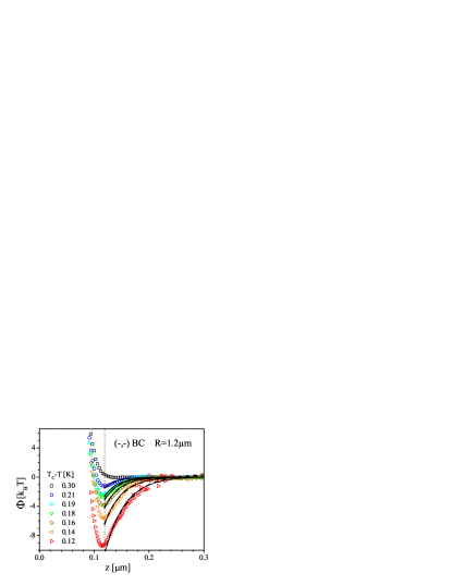
Figure 10: Effective interaction potential $\Phi(z)$ between a wall and a spherical particle of radius $1.2\,\mu$m immersed in a water-lutidine mixture at the critical concentration $c^{c}_{L}$, as a function of the distance $z$ from the wall and for various values of the temperature in the one-phase region ($T<T_{c}$) nature . The gravitational and the offset contribution to the potential [see Eq. (26)] have been subtracted. The set of solid and dashed lines, which are barely distinguishable on this scale, correspond to the theoretical predictions (see the main text for details). The potentials reported here refer to the ${(-,-)}$ boundary conditions (other cases are reported in Figs. 11 and 12) and show that an increasingly attractive force contributes to the total potential upon approaching the critical temperature, i.e., upon decreasing $\Delta T=T_{c}-T$. Here $T_{c}$ is the nominal value of the critical temperature, corresponding to the anomaly in the background scattering, which signals the onset of critical opalescence in the sample. Only the data to the right of the vertical dotted line are considered for the comparison with the theoretical predictions (see the main text).

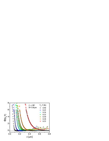
Figure 11: Interaction potential $\Phi(z)$ as in Fig. 10 for the ${(+,-)}$ boundary conditions and $R\simeq 1.85\,\mu$m nature . An increasingly repulsive force contributes to the total potential upon approaching the critical temperature. The set of solid and dashed lines, which are barely distinguishable on this scale, correspond to the theoretical predictions (see the main text for details). Only the data to the right of the vertical dotted line are considered for the comparison with the theoretical predictions (see the main text).

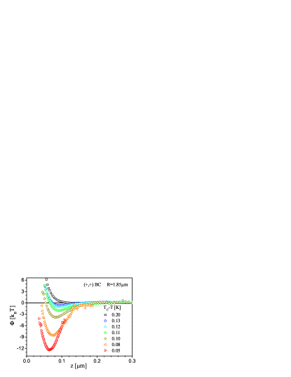
Figure 12: Interaction potential $\Phi(z)$ as in Figs. 10 and 11, for the ${(+,+)}$ boundary conditions nature . As for ${(-,-)}$ boundary conditions (see Fig. 10), upon approaching the critical temperature an increasingly attractive force contributes to the total potential.

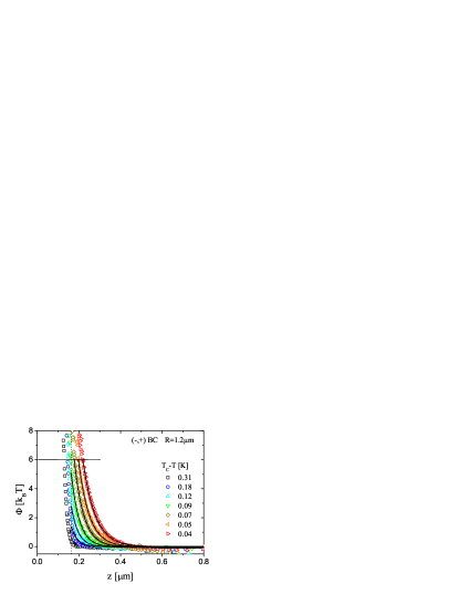
Figure 13: Interaction potential $\Phi(z)$ as in Figs. 10, 11, and 12 for the ${(-,+)}$ boundary conditions. As in the case of the ${(+,-)}$ boundary conditions (see Fig. 11) an increasingly repulsive force contributes to the total potential upon approaching the critical temperature. The set of solid and dashed lines, which are barely distinguishable on this scale, correspond to the theoretical predictions (see the main text for details). Only the data to the right of the vertical dotted line are considered for the comparison with the theoretical predictions (see the main text).

For the binary liquid mixture at the critical composition we have estimated (after data acquisition) the critical temperature $T_{c}$ as the temperature at which anomalies in the background light scattered by the mixture in the absence of the colloid and due to critical opalescence are observed and visual inspection of the sample displays an incipient phase separation. The value determined this way has to be understood as an estimate of the actual value of the critical temperature of the water-lutidine mixture and it is used for the calibration of the temperature scale, which is shifted in order to set $T_{c}$ to the nominal value $T_{c}=307.15\,$K reported in the literature (see, e.g., Ref. beysens1 ). Note, however, that depending on the different level of purity of the mixture, published experimental values of $T_{c}$ are spread over the range $306.54\div 307.26$ K (see, e.g., the summary in Ref. mb06 ). Due to the difficulties in determining the absolute value of the critical temperature, with our experimental setup only temperature differences are reliably determined and the actual critical temperature of the mixture might differ slightly from the nominal value $T_{c}$. We shall account for this fact in our comparison with the theoretical predictions.

Close to $T_{c}$ critical opalescence is expected to occur. It is indeed ultimately observed upon heating the mixture towards the critical temperature, leading to an increase in the background light scattering due to the correlated fluctuations in the mixture. Even though this might interfere with the determination of the interaction potential $\Phi$ via TIRM, within the range of temperatures we have explored at the critical concentration, the enhancement in the background scattering is actually negligible compared to the light scattered by the particle.

In Fig. 10 we present the interaction potentials $\Phi$ as a function of the distance $z$ for that choice of colloidal particle and surface treatment which realizes the ${(-,-)}$ boundary condition (see Tab. 1). As discussed above, for $\Delta T\equiv T_{c}-T=0.30$K, the potential consists only of the electrostatic repulsion (see Eq. (28)). Upon approaching the critical point an increasingly deep potential well gradually develops, indicating that an increasingly strong attractive force is acting on the particle. At the smallest $\Delta T$ we have investigated, i.e., $\Delta T=0.12$K, the resulting potential well is so deep that the particle hardly escapes from it. In view of the small temperature variation of ca. 180 mK, the change of ca. $10k_{\mathrm{B}}T$ in the resulting potential is remarkable. This very sensitive dependence on $T$ is a clear indication that in the present case critical Casimir forces are at work. In the case of Fig. 10 the maximum attractive force acting on the particle is about 600 fN.

According to the theoretical predictions, one expects the critical Casimir force to be repulsive for asymmetric boundary conditions ${(+,-)}$ or ${(-,+)}$. In our experiment we can easily realize the ${(+,-)}$ BC by changing the colloidal particle surface from preferentially adsorbing water $(-)$ to preferentially adsorbing lutidine $(+)$, without any additional surface treatment of the cell (see Tab. 1). The interaction potentials $\Phi$ for this case are reported in Fig. 11. As for the ${(-,-)}$ boundary condition, sufficiently far from the critical point (i.e., $\Delta T=T_{c}-T=0.90\,$K), the potential consists only of the electrostatic repulsion contribution [see Eq. (28)]. However, upon approaching the critical point the repulsive part of the potential curves shifts towards larger values of the distance $z$, indicating that an additional repulsive force is acting on the colloid. It is possible to make this force attractive again by treating the surface of the cell so that its preferential adsorption changes from water $(-)$ to lutidine $(+)$, so that then ${(+,+)}$ boundary condition is realized. As Fig. 12 shows, the resulting potentials show indeed an attractive part the qualitative features of which resemble those of the case with the ${(-,-)}$ boundary condition, reported in Fig. 10. Note that the depth of the potential in Fig. 12 corresponding to $\Delta T=0.05$ is so large that the gravitational part (which has been subtracted) cannot be sampled by the particle and therefore the position of this potential curve along the vertical axis cannot be fixed. If, with the same $(+)$ surface of the cell, one changes again the colloidal particle from preferentially adsorbing lutidine $(+)$ to preferentially adsorbing water $(-)$, we can experimentally realize the ${(-,+)}$ boundary condition (see Tab. 1) for which a repulsive critical Casimir force is expected. The resulting potential is reported in Fig. 13 and shows the same qualitative features as the one in Fig. 11, with an increasingly repulsive force which builds up upon approaching the critical point.

IV.2.2 Comparison with theory

The experimental data reported in the previous subsection can be compared with the theoretical predictions presented in Sec. II.1, which are expected to be valid for $\delta\equiv z/R\ll 1$ (Derjaguin approximation). In the experimental setting corresponding to Figs. 10 and 13, $R=1.2\mu$m whereas $z\lesssim 0.3\mu$m and $z\lesssim 0.8\mu$m, respectively, so that $\delta\lesssim 0.25$ and $\delta\lesssim 0.67$. In Figs. 11 and 12 one has $R\simeq 1.85\mu$m with $z\lesssim 0.8$ and $z\lesssim 0.3$, respectively, corresponding to $\delta\lesssim 0.43$ and $\delta\lesssim 0.16$. Accordingly the Derjaguin approximation is expected to provide a sufficiently accurate description of the experimental data, possibly apart from those at larger values of $z$ in Figs. 11 and 13, the corresponding potential values of which are anyhow negligibly small. In order to extract from the measured potential only the part which is due to the critical Casimir force we focus on that range of distances $z$ for which the electrostatic contribution $\Phi_{0}(z)$ (see Eqs. (26) and (28)) as measured far from the critical point (i.e., for $\Delta T=0.30$K in Fig. 10 and $\Delta T=0.90$K in Fig. 11) is actually negligible, using as a criterion $|\Phi_{0}(z)|\lesssim 0.5k_{\mathrm{B}}T$. This latter choice also avoids additional complications due to possible changes induced by critical fluctuations in the electrostatic contribution $\Phi_{0}(z)$ upon approaching the critical point. Accordingly, for a quantitative comparison with the theoretical predictions we consider only data corresponding to $z\geq 0.12\mu$m in Fig. 10 [${(-,-)}$ BC], $z\geq 0.1\mu$m in Fig. 11 [${(+,-)}$ BC], and $z\geq 0.16\mu$m in Fig. 13 [${(-,+)}$ BC], excluding in each case the data set corresponding to the largest value of $\Delta T$, which has been used to define $\Phi_{0}(z)$. Unfortunately, the number of data points which satisfy this condition in the case of Fig. 12 is quite limited for providing a basis for a reliable analysis; therefore we do not process these corresponding data.

The strength of the critical Casimir force depends strongly on the deviation $T_{c}-T$ from the critical point via the bulk correlation length $\xi\sim|T_{c}-T|^{-\nu}$. Accordingly, even a small systematic error in the experimental determination of $T$ and $T_{c}$ can result in sizeable discrepancies in the comparison between measured potentials and theoretical predictions. Statistical variations and a possible drift of the temperature during the acquisition of the data, which are kept within $5\,$mK by the temperature controller used in our experimental apparatus nature , are similarly important. In order to circumvent parts of these problems we compare the experimental data, selected by the aforemention criterion (see the vertical lines in Figs. 10, 11, and 13), for a certain boundary condition and for the six temperatures $T_{i}=T_{c}-\Delta T_{i}$, $i=1$,…, 6, closest to $T_{c}$ with the theoretical prediction for $\Phi_{C}(z;\xi)$ provided by Eqs. (12) and (13). For each $T_{i}$ the values $\xi_{i}$ of the correlation length and of a possible residual offset $\Phi_{{\rm offset},i}$ are determined in such a way as to optimize the agreement between $\Phi_{C}(z;\xi_{i})+\Phi_{{\rm offset},i}$ and the corresponding experimental data set. A drift of the temperature during the acquisition of the data might affect the value of the correlation length $\xi_{i}$ resulting from this procedure. As we shall see below, even if present, this possible drift does not strongly affect the final estimate for the correlation length amplitude $\xi_{0}$ in Eq. (2), the uncertainty of which is dominated by the systematic uncertainty of the theoretical predictions stemming from finite-size extrapolations of the Monte Carlo data.

The data set $(T_{i},\xi_{i})$ is then fitted with the theoretically expected power-law behavior given by Eq. (2). This is carried out by fixing the universal critical exponent $\nu\simeq 0.630$ to its best known theoretical value while determining the non-universal amplitude $\xi^{\rm(fit)}_{0}$ and the value $T_{c}^{\rm(fit)}$ of the critical temperature from the data set $(T_{i},\xi_{i})$:

$$\xi_{i}=\xi^{\rm(fit)}_{0}\left(1-\frac{T_{i}}{T_{c}^{\rm(fit)}}\right)^{-0.63}\,.$$ (32)

Here we assume that the temperatures $T_{i}$ are sufficiently close to $T_{c}$ so that $\xi$ is described correctly by its leading power-law behavior. The resulting value of $\xi^{\rm(fit)}_{0}$ can then be compared with the available independent experimental estimates reported in Tab. 3, providing a check of the consistency of the experimental data with the theoretical predictions.

$\xi^{\rm(exp)}_{0}\,$[Å]		Ref. (year)	Method
$2.0\phantom{0}$	$\pm 0.2$	gcsp72 (1972)	static LS
$2.92$	$\pm 0.19$	gcsp72 (1972)	dynamic LS, linewidth
$2.7\phantom{0}$	$\pm 0.2$	jbww87 (1987)	static LS
$2.3\phantom{0}$		elv93 (1993)	specific heat
$2.1\phantom{0}$		slsl97 (1997)	critical adsorption
$1.98$	$\pm 0.04$	mb06 (2006)	specific heat

Table 3: Experimental estimates of the non-universal correlation length amplitude $\xi_{0}$ for the water-lutidine mixture at the critical concentration. In light scattering (LS) experiments the bulk correlation length $\xi(T)$ is determined by measuring the wave-vector (static) or frequency (linewidth, dynamics) dependence of the scattered intensity. A fit of $\xi(T)$ to the expected algebraic behavior [Eq. (2)] yields the value $\xi_{0}$. Alternatively, $\xi_{0}$ can be obtained on the basis of the measured value of the non-universal amplitude $A^{+}$ which characterizes the divergence of the specific heat at constant pressure $C_{p}(\tau\rightarrow 0^{+})\simeq(A^{+}/\alpha)\tau^{-\alpha}$ and the theoretical mb06 or experimental elv93 value of the universal amplitude ratio $Q^{+}=A^{+}\xi_{0}^{3}\rho/(Mk_{\mathrm{B}})$, where $M$ is the molar mass of the mixture and $\rho$ its mass density at the critical point Priv ; PV . A careful theoretical analysis of experimental data for the critical adsorption profiles also leads to an estimate for $\xi_{0}$ slsl97 . Comparing the experimentally measured potentials to the theoretical predictions for the critical Casimir contribution we obtain the estimate reported in, c.f., Eq. (34).

In spite of the scattering of the available experimental data, which might be due to different conditions of the mixture (such as contaminations or slightly different concentrations) or to different systematic uncertainties of the various approaches, all the estimates are within the range

$$\xi^{\rm(exp)}_{0}=2.3\pm 0.4\,\mbox{\AA},$$ (33)

estimated via a least-square fit of the data mb06 ; gcsp72 ; jbww87 ; elv93 ; slsl97 in Tab. 3. (The experimental value quoted in Ref. nature refers to the estimate of Ref. gcsp72 .) The limited set of temperatures which have been investigated experimentally (apart from one far away from $T_{c}$ and used for fixing the background potential, six different values for each set of boundary conditions) does not allow us to determine simultaneously and reliably the exponent $\nu$ from the experimental data.

In comparing the experimental data with the theoretical predictions we have to take into account the uncertainties which affect both of them. As discussed in Sec. II.1 the currently available theoretical predictions within the Derjaguin approximation are affected by a 20% systematic uncertainty, clearly visible in Fig. 2, for the amplitude of the scaling function of the Casimir potential $\Phi_{C}$.

As far as the experimental data are concerned, the systematic uncertainties — which are the ones most relevant for the comparison — concern (i) the particle-wall distance $z$, which can be determined by the hydrodynamic method up to $\Delta z=\pm 30$nm (see Sec. III.1 and Ref. footnote1 ) and (ii) the absolute temperature scale $T$ and, in particular, the value of the critical temperature $T_{c}$. As described above, in order to cope with the uncertainty in $T$ we opted for an indirect determination of the associated correlation length from the best fit of the experimental data with theoretical predictions.

In addition to these systematic uncertainties, there are statistical errors associated with the way the potential $\Phi$ is determined via TIRM. The number $N(n_{\rm sc})$ of counts during the sampling time $t_{\rm samp}$, registered in each bin of size $\Delta n_{\rm sc}$, centered around $n_{\rm sc}$ and forming the intensity histogram $p_{\rm sc}(n_{\rm sc})=N(n_{\rm sc})/(N_{\rm tot}\Delta n_{\rm sc})$ reported in Fig. 6(b), is subject to statistical fluctuations $\Delta N(n_{\rm sc})$ which affect the estimate of $p_{\rm sc}(n_{\rm sc})$, $p_{z}(z)$, and therefore of the potential $\Phi$; $N_{\rm tot}=f_{\rm samp}t_{\rm samp}$ is the total number of counts in the time series of $n_{\rm sc}(t)$ of duration $t_{\rm samp}$, from which the histogram of $p_{\rm sc}(n_{\rm sc})$ has been constructed. One expects that these statistical fluctuations are relatively more important for those bins which are less populated, i.e., for smaller $N(n_{\rm sc})$. In terms of the distance $z$ of the colloid from the wall, they correspond to values which are less frequently sampled during the Brownian motion of the particle under the influence of the potential $\Phi$, i.e., to larger values of the potential. This can be seen directly from the potentials reported in Figs. 10, 11, 12, 13, and, c.f., 17, in which the experimental data are more scattered very close to the wall and far from it, whereas the sampling of the potential $\Phi$ is particularly accurate around its minimum. In order to evaluate the statistical uncertainty associated with each data point of the potential, ideally one should construct the histogram of $p_{\rm sc}(n_{\rm sc})$ based on several different realizations of the time series $n_{\rm sc}(t)$ and then analyze the statistical properties of this ensemble of plots. Alternatively, one might evaluate the autocorrelation time $t_{\rm corr}$ of $n_{\rm sc}(t)$ [e.g., from a detailed study of the autocorrelation function $C(\delta t)$, see the text before Eq. (25)]. Assuming that the number $N_{\rm in}(n_{\rm sc})$ of statistically independent counts in a bin of the histogram is given by $N_{\rm in}(n_{\rm sc})=N(n_{\rm sc})/(f_{\rm samp}t_{\rm corr})$ and assuming that the statistics of the counts is Poissonian, the associated relative statistical fluctuation is related to the number of counts by $\Delta N_{\rm in}(n_{\rm sc})=\sqrt{N_{\rm in}(n_{\rm sc})}$ and induces a statistical uncertainty $\Delta\Phi(z(n_{\rm sc}))/(k_{\mathrm{B}}T)=\Delta N_{\rm in}(n_{\rm sc})/N_{\rm in}(n_{\rm sc})=N^{-1/2}_{\rm in}(n_{\rm sc})$ for the value of the potential $\Phi$ at the position $z(n_{\rm sc})$ corresponding to the scattered number of photons $n_{\rm sc}$. However, in the comparison between the experimental data and the theoretical predictions, the statistical error in the former is expected to be negligible compared to the systematic uncertainty in the latter and therefore we do not proceed to a detailed evaluation of the statistical error associated with the data points reported in Figs. 10, 11, 12, 13 , and, c.f., 17. Actually, a good estimate of the magnitude of the statistical error can be inferred from the scatter of the experimental data points relative to a smooth curve interpolating each potential.

In order to discard those data which are affected by large statistical fluctuations, we consider for the comparison with the theoretical prediction only data fulfilling $\Phi(z)<6k_{\mathrm{B}}T$ and $z\leq z_{\rm max}$ where $z_{\rm max}=0.3\,\mu$m for Fig. 10,

$z_{\rm max}$ [$\mu$m]	0.3	0.35	0.35	0.4	0.5	0.8
$\Delta T$[K]	0.43	0.34	0.32	0.30	0.28	0.25

for Fig. 11, and

$z_{\rm max}$ [$\mu$m]	0.4	0.4	0.45	0.5	0.55	0.6
$\Delta T$[K]	0.18	0.12	0.09	0.07	0.05	0.04

for Fig. 13. For the ${(-,-)}$ boundary conditions, in Fig. 10 we report the comparison between the theoretical prediction and those experimental data which have been selected as explained above. The solid and dashed lines, barely distinguishable, correspond to the predictions given by Eq. (12) by using for $\Theta_{{(-,-)}}=\Theta_{{(+,+)}}$ the scaling functions described by the solid and dashed lines, respectively, in Fig. 2. (For each temperature $\Delta T_{i}$ the experimental potentials have been shifted vertically by the amount $-\Phi_{{\rm offest},i}$ determined previously as the best fit parameter.) The corresponding values $\xi_{i}$ of the correlation length are reported in Fig. 14 together with the resulting best fit based on Eq. (32),

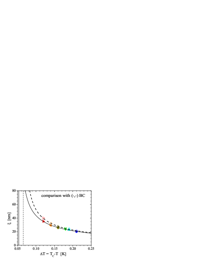
Figure 14: Correlation length $\xi$ as a function of the temperature deviation $\Delta T=T_{c}-T$ from the experimentally located critical temperature $T_{c}$ for the water-lutidine mixture at the critical concentration. The sets of data points are obtained by optimizing the agreement between the experimental data from Fig. 10 and the corresponding theoretical predictions for the Casimir potential for the ${(-,-)}$ boundary conditions (Fig. 2, see the main text for details). The upper (lower) set of points has been determined by using as the scaling function $\Theta_{{(-,-)}}=\Theta_{{(+,+)}}$ of the Casimir potential the one reported by the dashed (solid) line in Fig. 2. The dashed and solid curves are the best fit of the corresponding data sets based on Eq. (32) with the corresponding values $\Delta T_{c}^{\rm(fit)}=T_{c}-T_{c}^{\rm(fit)}$ indicated by the vertical dashed and solid lines, respectively, i.e., $\xi$ diverges at $T_{c}^{\rm(fit)}$ corresponding to $\Delta T(T=T_{c}^{\rm(fit)})=T_{c}-T_{c}^{\rm(fit)}=\Delta T_{c}^{\rm(fit)}$.

which leads to the least-square estimates $\xi_{0}^{\rm(fit)}=1.7\pm 0.1$Å and $\Delta T_{c}^{\rm(fit)}\equiv T_{c}-T_{c}^{\rm(fit)}=52\pm 10$ mK for the solid curve and $\xi_{0}^{\rm(fit)}=1.7\pm 0.1$Å and $\Delta T_{c}^{\rm(fit)}=65\pm 7$ mK for the dashed one. Taking into account the systematic uncertainty of the scaling functions for the Casimir potential, we arrive at the combined estimate $\Delta T_{c}^{\rm(fit)}=60\pm 15$ mK, i.e., the value of $T_{c}$ determined experimentally is actually higher than the value $T_{c}^{\rm(fit)}$ resulting from the comparison with the theoretical predictions. In addition, this comparison allows one to estimate the correlation length $\xi$, for which no independent experimental estimate is presently available. According to Fig. 14 one has $20\mbox{nm}\lesssim\xi\lesssim 40\mbox{nm}$, so that for the range $0.12\mu\mbox{m}\leq z\leq 0.3\mu\mbox{m}$ of distances this translates into the ranges $3\lesssim x=z/\xi\lesssim 15$ and $6\lesssim u=(1-T/T^{\rm(fit)}_{c})^{1/\nu}(z/\xi_{0}^{\rm(fit)})^{1/\nu}\lesssim 70$ of the scaling variables $x$ and $u$ (see Fig. 2). In order to be able to test prominent features of the theoretically predicted scaling function such as the occurrence of a minimum for $u_{\rm min}\simeq 0.5$, one has to reach $\xi\gtrsim 180$ nm, i.e., one must get still closer to the critical point ($\Delta T\lesssim 6\,$mK) than it was possible in the present experiment.

For the ${(+,-)}$ boundary conditions, in Fig. 11 we report the comparison between the theoretical prediction and those experimental data which have been selected as explained above. As in Fig. 10, the solid and dashed lines correspond to the predictions based on Eq. (12) by using for $\Theta_{{(+,-)}}=\Theta_{{(-,+)}}$ the scaling functions indicated as solid or dashed line, respectively, in Fig. 2. (As in Fig. 10, the experimental potentials have been shifted vertically for each temperature $\Delta T_{i}$ by the amount $-\Phi_{{\rm offest},i}$ determined previously as the best fit parameter.) The corresponding ensuing values $\xi_{i}$ of the correlation length are reported in Fig. 15, together with the resulting best fit based on Eq. (32),

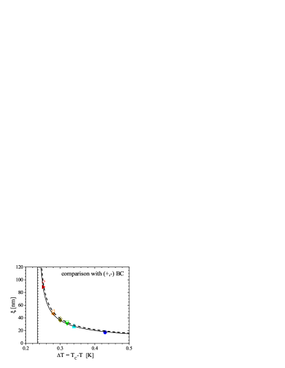
Figure 15: Same as Fig. 14, obtained by optimizing the agreement between the experimental data from Fig. 11 and the corresponding theoretical predictions for the critical Casimir potential for the ${(+,-)}$ boundary conditions (Fig. 2).

which leads to the least-square estimates $\xi_{0}^{\rm(fit)}=1.8\pm 0.1$Å and $\Delta T_{c}^{\rm(fit)}\equiv T_{c}-T_{c}^{\rm(fit)}=234\pm 2$mK for the solid curve and $\xi_{0}^{\rm(fit)}=1.9\pm 0.1$Å and $\Delta T_{c}^{\rm(fit)}=235\pm 2$mK for the dashed one. The final combined estimate of $\Delta T_{c}^{\rm(fit)}$, which takes into account the systematic uncertainty of the amplitude of the theoretical prediction of $\Theta_{{(+,-)}}$, is therefore $\Delta T_{c}^{\rm(fit)}=235\pm 3$ mK. The correlation lengths reported in Fig. 15 are in the range $20\mbox{nm}\lesssim\xi\lesssim 95\mbox{nm}$. The corresponding ranges of distances $z$ depend on the temperature $\Delta T$ (see Fig. 11) so that the experimental data cover the scaling variable ranges $3.4\lesssim x=z/\xi\lesssim 17$ and $7\lesssim u=(1-T/T^{\rm(fit)}_{c})^{1/\nu}(z/\xi_{0}^{\rm(fit)})^{1/\nu}\lesssim 85$ (see Fig. 2).

For the ${(-,+)}$ boundary conditions, in Fig. 13 we report the comparison between the theoretical prediction and those experimental data which have been selected as explained above. As in Figs. 10 and 11, the sets of solid and dashed lines, barely distinguishable, correspond to the predictions based on Eq. (12) by using for $\Theta_{{(-,+)}}=\Theta_{{(+,-)}}$ the scaling functions indicated as solid or dashed line, respectively, in Fig. 2. (As in Figs. 10 and 11, the experimental potentials have been shifted vertically for each temperature $\Delta T_{i}$ by the amount $-\Phi_{{\rm offest},i}$ determined previously as the best fit parameter.) The corresponding values $\xi_{i}$ of the correlation length, which can be inferred from this comparison, are reported in Fig. 16, together with the resulting best fit based on Eq. (32),

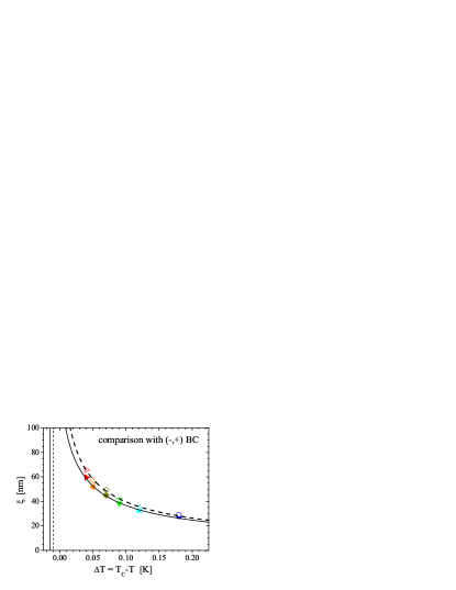
Figure 16: Same as Figs. 14 and 15, obtained by optimizing the agreement between the experimental data from Fig. 13 and the corresponding theoretical predictions for the critical Casimir potential for the ${(-,+)}$ boundary conditions (Fig. 2).

which leads to the least-square estimates $\xi_{0}^{\rm(fit)}=2.55\pm 0.25$Å and $\Delta T_{c}^{\rm(fit)}\equiv T_{c}-T_{c}^{\rm(fit)}=14\pm 11\,$mK for the solid curve and $\xi_{0}^{\rm(fit)}=2.7\pm 0.2$Å and $\Delta T_{c}^{\rm(fit)}\equiv T_{c}-T_{c}^{\rm(fit)}=10\pm 9\,$mK for the dashed one. The final combined estimate of $\Delta T_{c}^{\rm(fit)}$, which takes into account the systematic uncertainty of the amplitude of the theoretical prediction of $\Theta_{{(-,+)}}$, is therefore $\Delta T_{c}^{\rm(fit)}=14\pm 11\,$mK. The correlation lengths reported in Fig. 16 are in the range $28\,\mbox{nm}\lesssim\xi\lesssim 66\,\mbox{nm}$ with the corresponding ranges of the distances $z$ depending on the temperature $\Delta T$ (see Fig. 13) so that the experimental data cover the scaling variable ranges $7\lesssim x=z/\xi\lesssim 67$ and $22\lesssim u=(1-T/T^{\rm(fit)}_{c})^{1/\nu}(z/\xi_{0}^{\rm(fit)})^{1/\nu}\lesssim 790$ (see Fig. 2).

The experimental data reported in Fig. 13 (which Fig. 16 refers to) have actually been acquired by an experimental setup which makes use of an improved temperature control compared to the one used during the acquisition of the data reported in Figs. 10, 11, 12, and 17. This upgrade of the setup is characterized by a better temperature stability and allows one to determine $T_{c}$ with higher accuracy nhb-09 .

As far as the value of $\xi_{0}$ is concerned, taking into account the values reported above for the ${(-,-)}$ and ${(+,-)}$ boundary conditions, one obtains the combined estimate $\xi_{0}^{\rm(fit)}=1.8\pm 0.2$ Å  nature which is in very good agreement with the experimental value $\xi_{0}^{\rm(exp)}$ reported in the first line of Tab. 3 (and quoted in Ref. nature ). It is interesting to note that the principal source of error in these estimates of $\xi_{0}$ is actually the systematic uncertainty in the theoretical predictions, which turns out to be more significant than the statistical or possible systematic experimental errors, such as the one due to possible variations or fluctuations of the temperature occurring during the measurement. Actually, due to the pronounced dependence of the theoretical predictions on the temperature via the correlation length, these variations should result in averaged effective values of the correlation length, most probably affecting the overall amplitude, i.e., the value of $\xi_{0}^{\rm(fit)}$. The estimate of $\xi_{0}^{\rm(fit)}=2.6\pm 0.3\,$Å based on the data for the ${(-,+)}$ boundary conditions agrees with the estimate reported in the third line of Tab. 3 but it is larger and not quite compatible with the former one. This might be due to larger systematic errors in the latter or due to possibly different conditions of the mixture employed in the experiment (e.g., purity or possible contamination by leaching). The combined estimate which accounts for the results of our analysis is therefore

$$\xi_{0}^{\rm(fit)}=2.2\pm 0.6\,\mbox{\AA},$$ (34)

which is compatible and similar to the experimental value $\xi_{0}^{\rm(exp)}$ reported in Eq. (33) but carrying a larger, mainly systematic, uncertainty. This agreement is particularly significant if one takes into account the fact that Eq. (34) combines results obtained from different experimental conditions (different particles and different surface treatments), interpreted on the basis of the available theoretical predictions. It is worthwhile to point out that one can equally reverse the line of reasoning given above. One can adopt the point of view that the correlation length is a bulk property which is determined by independent bulk measurement yielding Eqs. (2) and (33). This way $\xi$ is not a fit parameter but an input which fixes the theoretical prediction for the critical Casimir potential completely. Since $\xi_{0}^{\rm(exp)}$ equals $\xi_{0}^{\rm(fit)}$, this implies that with this fixed input the theoretical predictions yield the solid and dashed lines in Figs. 10, 11, and 13. In this sense one can state that the remarkable agreement between theory and experiment observed in the figures occurs without adjusting parameters.

IV.3 Noncritical composition

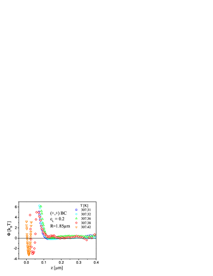
Figure 17: Effective interaction potential $\Phi(z)$ between a wall and a particle of diameter $2R=3.69\,\mu$m, immersed in a water-lutidine mixture at mass fraction $c_{L}=0.2<c_{L}^{c}$, as a function of the distance $z$ and for various values of the temperature close to the demixing phase boundary nature . This system corresponds to the ${(+,+)}$ boundary conditions. The gravitational and offset contributions to the potential [see Eq. (26)] have been subtracted. The abrupt formation of a narrow minimum of the potential close to the wall upon increasing the temperature is interpreted as the formation of a liquid bridge between the particle and the wall (see the main text).

In the sense of renormalization-group theory the deviation of the bulk concentration $c_{L}$ from its critical composition $c_{L}^{c}$ represent the second relevant scaling field besides the reduced temperature. In the language of the Ising universality class the field conjugate to this deviation plays the role of a bulk magnetic field. (Here we do not discuss that actually two linear combinations of the conjugate field and of the reduced temperature form the appropriate orthogonal scaling fields.) In this sense, as already mentioned in Sec. II.2, measurements along thermodynamic paths of varying temperature at fixed off-critical compositions probe the dependence of the critical Casimir forces on another, equally important scaling variable. Corresponding theoretical predictions have been derived for the parallel-plate geometry f-th as well as for two adjacent spherical particles colloids1a ; colloids1b ; one expects that a similar behavior holds for the present geometry of a sphere near a planar surface. For a composition of the binary liquid mixture far away from its critical value the critical Casimir forces become negligible. For small deviations from the critical lutidine mass fraction $c_{L}^{c}$ and for the ${(+,+)}$ BC (so that both surfaces preferentially adsorb lutidine) the temperature variation of the Casimir force upon approaching the two-phase coexistence line near the critical point from the mixed phase depends on whether $c_{L}$ is larger or smaller than $c_{L}^{c}$. If $c_{L}$ is slightly less than the critical composition, $c_{L}\lesssim c_{L}^{c}$, the Casimir force is expected to behave similarly as along the critical composition, i.e., it should exhibit a minimum before reaching the temperature $T_{*}(c_{L})$ at which phase separation occurs [$T_{*}(c_{L}=c_{L}^{c})=T_{c}$]. However, the depth of the critical Casimir potential is expected to be considerably deeper away from the critical composition (see Fig. 8 in Ref. colloids1b ). For lutidine mass fractions slightly larger then the critical value, $c_{L}>c_{L}^{c}$, as function of temperature the Casimir force is expected to vary similarly as in the case $c_{L}<c_{L}^{c}$ but much weaker.

These expectations are in agreement with the observations made in our experiment for the ${(+,+)}$ BC and for several values of lutidine mass fractions in the range $0.26<c_{L}<0.32$ [not shown]. For $c_{L}$ close to $c^{c}_{L}$ the measured potentials between the wall and the colloidal particle look similar to those obtained for the critical composition. For $c_{L}$ much smaller than $c^{c}_{L}$ the potentials are similar to the ones shown in Fig. 17 (see, e.g., Fig. 6.9 in Ref. h-th , corresponding to $c_{L}\simeq 0.25$).

For the values of $c_{L}$ further away from $c_{L}^{c}$ the system is no longer near criticality. Therefore the critical Casimir force ceases to influence effective interactions between the colloidal particle and the wall. However, for the ${(+,+)}$ BC and for temperatures allowing for phase separation, i.e., in the present case above the critical temperature, one expects a bridging transition to occur at compositions $c_{L}<c_{L}^{c}$. If the lutidine concentration is below its critical value $c_{L}^{c}$ the conjugate bulk field favors the water-rich phase whereas for the ${(+,+)}$ BC the confining surfaces prefer the lutidine-rich phase. At a single wall this competition gives rise to wetting phenomena and in confined geometries to condensation phenomena. As discussed in detail in Sec. II.2, if a bridge of the condensing phase connects two adjacent spheres immersed in the binary liquid mixture, there is an attractive wetting-induced interaction that pulls the sphere together. We expect a similar scenario to occur for the present geometry, i.e., if a wetting bridge of the phase which is favored by both surfaces is formed between the spherical particle and the planar wall.

Indeed, the measurements carried out for lutidine mass fractions $c_{L}\lesssim 0.2$ indicate that such a bridge formation takes place. In Fig. 17 we plot the measured particle-wall interaction potentials at several temperatures near but below the temperature of demixing $T_{*}(c_{L}=0.2)$, which could not be located with sufficient accuracy. Moreover, the temperature scale in Fig. 17 has not been calibrated with a reference temperature, so that only temperature changes are significant. As one can see for temperatures between 307.31 and 307.36 K, the potentials are very well described by Eq. (26) which accounts for the electrostatic and gravitational contributions only. However, upon further increasing the temperature by 20 mK we observe a markedly different behavior of the potentials. Suddenly the interaction potentials are shifted towards smaller values of distances $z$. Also the shape is changed in that the potentials exhibit a narrow and deep minimum. This sudden shift of the potential well towards the surface indicates the onset of an attractive interaction between the particle and the wall. A further slight increase in temperature gives rise to an even stronger shift of the potential minimum towards the wall. This phenomenon is observed only for lutidine mass fractions smaller than the critical value, i.e., on that side of the phase diagram where the mixture is poor in the component that is preferentially adsorbed by both surfaces. This behavior is in stark contrast to critical Casimir forces which vary gradually as function of the thermodynamic variables. On the other hand, for the ${(-,-)}$ boundary conditions and $c_{L}\gtrsim c_{L}^{c}$ the resulting potentials do not differ qualitatively from those shown in Fig. 10. But by further increasing the concentration of lutidine to $c_{L}=0.4$ one observes the sudden formation of a narrow and deep potential well upon increasing the temperature (see the potential corresponding to $c_{L}=0.3$, $0.32$, and $0.4$, reported in Fig. 6.11 of Ref. h-th ). These observations are in agreement with the theoretical concepts described in Sec. II.2. The effective potentials associated with the formation of a bridge, formed by the phase coexisting with the bulk phase, between the particle and the substrate are theoretically expected to exhibit hysteresis upon changing the temperature back towards its start value. However, in the present experiment, only rather weak hints for this hysteresis have been observed and actually no convincing evidence for it could be produced.

V Summary, conclusions, perspectives, and applications

V.1 Summary

We have presented a detailed account of the experimental and theoretical investigations of the effective forces acting on spherical colloidal particles of radius $R$ close to a substrate and immersed in a near-critical binary liquid mixture, shortly reported in Ref. nature . Based on total internal reflection microscopy (Figs. 5, 6, and 7) our main experimental findings are the following:

1. Upon raising the temperature $T$ of the binary liquid mixture of water and lutidine at its critical concentration towards its lower critical point $T_{c}$ of demixing (see Fig. 8), an attractive or repulsive force acting on the colloidal particle arises gradually.

2. This effective force is attractive if the surfaces of the colloid and of the substrate display preferential adsorption of the same component of the mixture (see Figs. 10 and 12), whereas it is repulsive in the cases of opposing preferences (see Figs. 11 and 13). This contribution to the total effective force (compare Sec. IV.1 and Fig. 9) is negligible at temperatures a few hundred mK away from $T_{c}$ and it increases significantly upon approaching it. As experimentally verified, these so-called critical Casimir forces can be reversibly switched on and off by changing the temperature.

3. If the concentration of this binary liquid mixture is close to but not equal to the critical one we have observed a behavior which is qualitatively similar to the one observed for the mixture at its critical concentration. In the close vicinity of the critical point there is no experimental evidence for the occurrence of wetting phenomena.

4. If the concentration of the binary liquid mixture differs significantly from the critical one and both surfaces exhibit the same preferential adsorption for that component of the mixture which is disfavored in the bulk, we observe the abrupt formation of a narrow and deep potential well (see Fig. 17) upon approaching the phase boundary of first-order demixing.

The experimental observations 1, 2, and 3 can be consistently interpreted in terms of the occurrence of the critical Casimir effect in near-critical mixtures, whereas observation 4 can be understood in terms of the formation of a bridgelike configuration of the segregated phases (see Fig. 4). For mixtures at the critical concentration it is possible to quantitatively compare the measured potentials with the corresponding theoretical predictions for the contribution of critical Casimir forces (see Eqs. (10) and (12) as well as Figs. 2 and 3), derived within the Derjaguin approximation (see Fig. 1) and for the range of distances within which electrostatic forces are negligible (see the solid lines in Figs. 10, 11, and 13). The correlation length $\xi$, as determined from the comparison between the experimental data and the theoretical predictions, follows rather well the theoretically expected universal power-law behavior (see Figs. 14, 15, and 16) and the associated non-universal amplitude $\xi_{0}$ is in agreement with previous independent experimental determinations for this specific binary mixture [compare Eq. (34) to Eq. (33) and see Tab. 3].

The same critical Casimir forces, investigated here by using a water-lutidine mixture, are expected to act on a colloid immersed in any binary liquid mixture close to its demixing point (or in any fluid close to its gas-liquid critical point) and in the vicinity of a substrate. While the values of non-universal parameters, such as $T_{c}$ and $\xi_{0}$, depend on the specific mixture, the resulting critical Casimir force is described by a material-independent, universal scaling behavior (see Eq. (3)) and scaling function (see Eq. (5) and Fig. 3 for small particle-substrate separation) which depends only on whether the adsorption preferences of the particle and of the substrate are equal $[{(+,+)},{(-,-)}]$ or opposite $[{(+,-)},{(-,+)}]$.

V.2 Discussion

The experimental observations summarized above might contribute to the understanding of the reversible aggregation of a dilute suspension of colloidal particles immersed in a water-lutidine mixture close to its demixing point, which has been the subject of several experimental studies since it was first observed in 1985 beysens1 (for a review see Ref. beysens2 ). The formation of pre-wetting layers around the particles was first invoked as a possible explanation for this phenomenon. Later on it was experimentally demonstrated that aggregation might actually occur in a region of the phase diagram which extends too far from the two-phase coexistence line and from the wetting transition to be possibly related to pre-wetting phenomena gkm-92 . (However, no aggregation was observed for mixtures at the critical concentration gkm-92 .) Among the possible different mechanisms (see, e.g., Ref. PLB-98 for a summary) which might contribute to explain this flocculation, also critical Casimir forces have been invoked theoretically, as summarized and discussed in Refs. colloids1a ; colloids1b ; colloids2 . In particular, the experimental observation (besides for 2,6-lutidine and normal water as solvent reported also for colloids dispersed in mixtures of 3-methylpyridine, heavy, and normal water nkg-93 ; saxs or 2-butoxyethanol and normal water gw-97 ) that flocculation phenomena are enhanced near but off the critical point, at compositions which are slightly poorer in the component preferentially adsorbed by the colloids than the critical one, matches with the fact that also the critical Casimir forces attain their maximum values there. Although flocculation involves the interaction of many colloidal particles and therefore is a many-body phenomenon (which can also be interpreted as a genuine phase transition in a ternary mixture jk-97 ), some features such as the experimentally determined asymmetry of the aggregation line with respect to the critical concentration (see, e.g., Refs. beysens1 ; gkm-92 ) can be qualitatively accounted for by the behavior of the effective interaction among two colloids, mediated by the near-critical solvent. This problem was theoretically investigated in Refs. colloids1a ; colloids1b ; colloids2 within various approximations. In this context, our experimental study of the interaction between a single colloidal particle and a substrate suggests that the actual magnitude of the forces due to the critical Casimir effect and due to the formation of a bridgelike configuration are large enough to play an important role also in aggregation phenomena. This has been demonstrated recently on patterned substrates patt-exp ; Tr-09 . However, more quantitative corresponding statements require additional dedicated studies of many-body effects. We note that, depending on the specific physical and chemical properties of the colloidal suspension under consideration, various mechanisms might be at play in determining its aggregation, especially for charged colloids, for which screening effects or even field-induced phase separation of the mixture might be predominant PLB-98 ; Tso-07 . In this respect, recent experimental studies of the structure factor of such an aggregating colloidal suspension via synchrotron small angle X-ray scattering (SAXS) saxs might provide important insight into the physical mechanisms at play in that phenomenon.

At the critical composition, the present experimental study detected the occurrence of critical Casimir forces in a range of distances $z$ which corresponds to a scaling variable $x=z/\xi\gg 1$. In this limit, some of the qualitative features of the scaling function of the force (such as the occurrence of a maximum for ${(+,+)}$ boundary conditions — see Fig. 3) have not been probed. Actually, in this limit the associated potential for $(+,\pm)$ boundary conditions is very well described by an exponential function $\Phi_{\mathrm{C}}(z)/(k_{\mathrm{B}}T)\simeq 2\pi A_{\pm}(R/\xi)\exp(-z/\xi)$ [see Eqs. (12) and (14)]. A clear signature of the collective nature of such an interaction is the fact that its range is set by the correlation length $\xi$. On the other hand, the functional form of this dependence on $z$ is quite generic and actually is common to interactions of rather different nature (e.g., electrostatic ones – see Eq.(28) – the range of which is set by the screening length $\kappa^{-1}$). For a relatively small correlation length $\xi\simeq\kappa^{-1}$ the critical Casimir interaction and the electrostatic repulsion have the same range and, depending on the specific values of the parameters, one of them might dominate over the other. Especially in this case one expects an interplay between these two effects due to the fact that the order parameter profile develops inhomogeneities on a length scale $\xi$ which is comparable to the typical length $\kappa^{-1}$ which characterizes the electrostatic screening in the homogeneous medium. Taking into account that due to the segregation of the mixture the ions have different solubilities in water and lutidine, the enhancement of one of these two components close to the confining surfaces might result in a change of the screening of the electrostatic interaction compared to the case of a non-critical homogeneous medium. Analogously, as dispersion forces depend sensitively on the spatial structure of the dielectric media forming the system and on the associated permittivities $\varepsilon(\omega,{\bf x})$, the inhomogeneities which build up in the medium upon increasing $\xi$ might affect significantly the background van-der-Waals contribution $\Phi_{0,{\rm vdW}}$ to the total potential compared to the estimate we gave for a homogeneous mixture [see Eqs. (27) and (29)]. In contrast to the critical Casimir effect, however, a quantitative analysis of the interesting interplay between critical fluctuations and dispersion/electrostatic forces necessarily requires the knowledge of several system-specific properties such as the actual spatially varying composition of the mixture and the resulting permittivity $\varepsilon(\omega,{\bf x})$. Some of these properties might be inferred experimentally via, e.g., surface plasmon spectroscopy of the binary mixture close to the substrate. The comparison of the experimental evidences presented here with the theoretical predictions has not generated an actual need to account for the possible interplays mentioned above. Presumably they result into effects which are negligible in the range of variables explored in our experiment and within our experimental accuracy. This might not be the case for different choices of the particle and the mixture for which, e.g., dispersion forces and therefore their possible modification due to critical fluctuations might be more relevant than in the system investigated here.

In order to compare the experimental data with the theoretical predictions we have inferred the bulk correlation length $\xi$ from the experimental data for the critical Casimir potential (see Sec. IV.2). Reversing the line of argument, $\xi$ can be inferred on the basis of the deviation $\Delta T$ from the critical temperature and of the knowledge of the non-universal amplitude $\xi_{0}$ which has been determined by independent bulk experiments. However, one could also determine the scaling functions of the critical Casimir potentials on the sole basis of experimental data, without need of any additional theoretical information. This requires the experimental determination of the actual correlation length $\xi$ corresponding to each temperature, which can be accomplished, e.g., by studying the light scattered by the mixture sufficiently far from the colloid and the substrate, probing the behavior of bulk fluctuations. Such an independent experimental determination of the scaling function would provide an additional, valuable test of the theoretical predictions.

V.3 Perspectives and applications

Suitable chemical treatments of the surfaces in contact with the binary liquid mixture can be used in order to control the strength of their preferential adsorptions (i.e., the corresponding surface fields, see Sec. II.1) and therefore the resulting critical Casimir force. The experimental data presented here have been consistently interpreted in terms of the theoretical predictions corresponding to strong preferential adsorption. However, in view of possible applications of these effective forces, it is also important to study in detail both experimentally patt-exp and theoretically patt-chem ; M-08 ; SD-08 ; Tr-09 cases in which such a preference is weaker or spatially modulated in a controllable fashion via suitable chemically patterned substrates. In the latter case and depending on the symmetry of the pattern, the resulting critical Casimir force acting on the colloidal particle acquires a lateral component in addition to the normal one investigated here patt-exp ; Tr-09 . This lateral force, as the normal one, is characterized by a universal scaling behavior and its range is again set by the correlation length $\xi$, such that it can be switched on and off by controlling the distance from the critical point. In addition, the force turns out to be rather sensitive to details of the imprinted chemical structure, e.g., the striped pattern considered in Refs. patt-exp ; Tr-09 . A proper theoretical analysis of the critical Casimir potential enables one to infer from the experimental data knowledge about such details even if they could not be determined by independent means, such as atomic force microscopy Tr-09 .

The lateral Casimir force might also find applications in colloid rheology. Consider, e.g., a dilute suspension of $(+)$ colloids exposed to a suitably fabricated substrate which has an adsorption preference smoothly varying along one direction from $(-)$ to $(+)$, such that it changes appreciably on the scale of the radius of the colloid. For sufficiently small values of the correlation length, the colloids diffuse isotropically along the substrate. However, upon approaching the critical point, the lateral Casimir force associated with the spatial gradient of the preferential adsorption (i.e., of the corresponding surface field) adds a deterministic drift to this diffusion process, resulting in a transport of colloids along the surface of the substrate. The direction of the flow will be reversed by changing the preferential adsorption of the colloid from $(+)$ to $(-)$, which can be exploited as a reversible selection mechanism. In this context, the critical Casimir force acting on a micrometer-sized colloid exposed to a substrate with a modulated adsorption preference on the the scale of some hundred micrometers has been recently studied experimentally nhb-09 .

Topographical modulations of the surface of an otherwise chemically homogeneous substrate can also be used to control the direction of the total force acting on a similar substrate patt-top or on a colloidal particle exposed to it. Additionally, chemical patterning or geometrical deviations from spherical symmetry of the colloidal particle (e.g., ellipsoidal colloids) result in a critical Casimir torque eisen ; khd-08 if the particle is exposed to a substrate. Combining all these features one should be able, e.g., to control reversibly via minute temperature changes the orientation of such colloids exposed to a striped substrate.

The critical Casimir force acting on a colloidal particle close to a plate fluctuates in time due to the fact that it originates from time-dependent critical fluctuations. In the present analysis we focused on the mean value of such a force and on the associated averaged potential $\Phi_{\mathrm{C}}$. However, as explained in Sec. (III.1), TIRM naturally provides a measurement of the time-dependent sphere-plate distance $z(t)$ which, in turn, can be used to determine the correlation time $t_{\rm R}$ of the critical Casimir force and how its expected algebraic temporal singularity builds up upon approaching the critical point. (Some aspects of this dynamical behavior are discussed in Refs. gd-06 ; g-08 ; gam-08 .) This critical slowing down of the critical Casimir effect can in principle be exploited in order to control the resulting dynamics of the colloidal particle.

In contrast to interactions which typically act among colloids (such as electrostatic and dispersion forces), the critical Casimir force is characterized by a pronounced temperature dependence. This fact can possibly be exploited in order to control via minute temperature changes the phase behavior and aggregation phenomena in colloidal dispersions in the bulk or close to those chemically structured solid surfaces which find applications in the fabrication of nano- and micrometer scale devices. Not only the range of the resulting interaction can be controlled but also its sign and spatial direction. This can be typically achieved by surface treatments and it does not require (as it does, e.g., for dispersion forces) substantial changes or a fine tuning of the bulk properties of the materials which constitute the immersed objects and the mixture itself. These properties could be used, e.g., in order to neutralize the attractive quantum mechanical Casimir force responsible for the stiction which brings micro-electromechanical systems to a standstill. If these machines would work not in a vacuum but in a liquid mixture close to the critical point, the stiction could be prevented by tuning the critical Casimir force to be repulsive via a suitable coating of the various machine parts. With optically removable or controllable coatings, one could very conveniently control the functioning of the microdevice without acting directly on it. In addition, properly designed surfaces might provide temperature-controlled confining potentials which might find applications in self-assembly processes patt-exp .

- (1) H. B. Casimir, Proc. K. Ned. Akad. Wet. 51, 793 (1948).
- (2) M. E. Fisher and P. G. de Gennes, C. R. Acad. Sci. Paris Ser. B 287, 207 (1978).
- (3) M. Krech, Casimir Effect in Critical Systems (World Scientific, Singapore, 1994); J. Phys.: Condens. Matter 11, R391 (1999).
- (4) G. Brankov, N. S. Tonchev, and D. M. Danchev, Theory of Critical Phenomena in Finite-Size Systems (World Scientific, Singapore, 2000).
- (5) J. N. Munday, F. Capasso, and V. A. Parsegian, Nature 457, 170 (2009).
- (6) K. Binder, in Phase Transitions and Critical Phenomena, edited by C. Domb and J. L. Lebowitz (Academic, London, 1983), Vol. 8, p. 1.
- (7) H. W. Diehl, in Phase Transitions and Critical Phenomena, edited by C. Domb and J. L. Lebowitz (Academic, London, 1986), Vol. 10, p. 76.
- (8) H. W. Diehl, Int. J. Mod. Phys. B 11, 3503 (1997).
- (9) M. Krech and S. Dietrich, Phys. Rev. Lett. 66, 345 (1991).
- (10) M. Krech and S. Dietrich, Phys. Rev. A 46, 1886 (1992).
- (11) A. Pelissetto and E. Vicari, Phys. Rep. 368, 549 (2002).
- (12) V. Privman, P. C. Hohenberg, and A. Aharony, in Phase Transitions and Critical Phenomena, edited by C. Domb and J. L. Lebowitz (Academic, New York, 1991), Vol. 14, p. 1 and p. 364.
- (13) M. Krech, Phys. Rev. E 56, 1642 (1997).
- (14) Z. Borjan and P. J. Upton, Phys. Rev. Lett. 81, 4911 (1998); ibid. 101, 125702 (2008).
- (15) O. Vasilyev, A. Gambassi, A. Maciołek, and S. Dietrich, Europhys. Lett. 80, 60009 (2007).
- (16) O. Vasilyev, A. Gambassi, A. Maciołek, and S. Dietrich, Phys. Rev. E 79, 041142 (2009).
- (17) M. Tröndle, L. Harnau, and S. Dietrich, J. Chem. Phys. 129, 124761 (2008).
- (18) M. Sprenger, F. Schlesener, and S. Dietrich, Phys. Rev. E 71, 056125 (2005); J. Chem. Phys. 124, 134703 (2006).
- (19) A. Hanke, F. Schlesener, E. Eisenriegler, and S. Dietrich, Phys. Rev. Lett. 81, 1885 (1998).
- (20) F. Schlesener, A. Hanke, and S. Dietrich, J. Stat. Phys. 110, 981 (2003).
- (21) M. Krech and S. Dietrich, Phys. Rev. A 46, 1922 (1992).
- (22) A. Gambassi, J. Phys.: Conf. Ser. 161, 012037 (2009).
- (23) S. Dietrich, in Phase Transitions and Critical Phenomena, edited by C. Domb and J. L. Lebowitz (Academic, London, 1988), Vol. 12, p. 1.
- (24) R. Garcia and M. H. W. Chan, Phys. Rev. Lett. 83, 1187 (1999); A. Ganshin, S. Scheidemantel, R. Garcia, and M. H. W. Chan, Phys. Rev. Lett. 97, 075301 (2006).
- (25) R. Garcia and M. H. W. Chan, Phys. Rev. Lett. 88, 086101 (2002).
- (26) M. Fukuto, Y. F. Yano, and P. S. Pershan, Phys. Rev. Lett. 94, 135702 (2005).
- (27) S. Rafaï, D. Bonn, and J. Meunier, Physica A 386, 31 (2007).
- (28) A. Hucht, Phys. Rev. Lett. 99, 185301 (2007).
- (29) M. Hasenbusch, preprint arXiv:0905.2096 (2009); preprint arXiv:0907.2847 (2009).
- (30) D. Dantchev and M. Krech, Phys. Rev. E 69, 046119 (2004).
- (31) R. Zandi, J. Rudnick, and M. Kardar, Phys. Rev. Lett. 93, 155302 (2004).
- (32) A. Maciołek, A. Gambassi, and S. Dietrich, Phys. Rev. E 76, 031124 (2007).
- (33) R. Zandi, A. Shackell, J. Rudnick, M. Kardar, and L. P. Chayes, Phys. Rev. E 76, 030601(R) (2007).
- (34) A. Maciolek and S. Dietrich, Europhys. Lett. 74, 22 (2006).
- (35) S. Kondrat, L. Harnau, and S. Dietrich, preprint arXiv:0907.1619 (2009)
- (36) E. Eisenriegler, J. Chem. Phys. 121, 3299 (2004); ibid. 124, 144912 (2006).
- (37) C. Hertlein, L. Helden, A. Gambassi, S. Dietrich, and C. Bechinger, Nature 451, 172 (2008).
- (38) A. Gambassi, C. Hertlein, L. Helden, C. Bechinger, and S. Dietrich, Europhysics News 40/1, 18 (2009).
- (39) T. W. Burkhardt and E. Eisenriegler, Phys. Rev. Lett. 74, 3189 (1995).
- (40) M. Tröndle, S. Kondrat, A. Gambassi, L. Harnau, and S. Dietrich, preprint arXiv:0903.2113v1 (2009).
- (41) M. Schlossman, X.-L. Wu, and C. Franck, Phys. Rev. B 31, 1478 (1985).
- (42) G. Flöter and S. Dietrich, Z. Phys. B 97, 213 (1995).
- (43) T. Mohry, diploma thesis, University of Stuttgart (2008).
- (44) F. M. Schmidt and H. W. Diehl, Phys. Rev. Lett. 101, 100601 (2008).
- (45) U. Ritschel and P. Czerner, Physica A 237, 240 (1997); Phys. Rev. Lett. 77, 3645 (1996).
- (46) S. Leibler and L. Peliti, J. Phys. C.: Solid State Phys. 30, L403 (1982); E. Brézin and S. Leibler, Phys. Rev. B 27, 594 (1983).
- (47) M. Smock, H. W. Diehl, and D. P. Landau, Ber. Bunsenges. Phys. Chem. 86, 486 (1994) [cond-mat/9402068].
- (48) H. B. Tarko and M. E. Fisher, Phys. Rev. Lett. 31, 926 (1973); Phys. Rev. B 11, 1217 (1975).
- (49) A. Drzewiński, A. Maciołek, and R. Evans, Phys. Rev. Lett. 85, 3079 (2000); A. Maciołek, A. Drzewiński, and R. Evans, Phys. Rev. E 64, 056137 (2001).
- (50) see, e.g., R. Evans, J. Phys.: Condens. Matter 2, 8989 (1990), and references therein.
- (51) T. Bieker and S. Dietrich, Physica A 252, 85 (1998); and references therein.
- (52) C. Bauer, T. Bieker, and S. Dietrich, Phys. Rev. E 62, 5324 (2000).
- (53) H. T. Dobbs, G. A. Darbellay, and J. M. Yeomans, Europhys. Lett. 17, 439 (1992).
- (54) D. Andrienko, P. Patricio, and O. I. Vinogradova, J. Chem. Phys. 121, 4414 (2004).
- (55) H. Shinto, K. Uranishi, H. Miyahara, K. Higashitani, J. Chem. Phys. 116, 9500 (2002).
- (56) D. Beysens and D. Estéve, Phys. Rev. Lett. 54, 2123 (1985).
- (57) D. Beysens, J. -M. Petit, T. Narayan, A. Kumar, and M. L. Broide, Ber. Bunsenges. Phys. Chem. 98, 382 (1994).
- (58) J. Y. Walz, Curr. Opin. Colloid Interface Sci. 2, 600 (1997).
- (59) D. C. Prieve, Adv. Colloid Interf. Sci. 82, 93 (1999).
- (60) L. Helden, E. Eremina, N. Riefler, C. Hertlein, C. Bechinger, Y. Eremin, and T. Wriedt, Applied Optics 45, 7299 (2006).
- (61) C. Hertlein, N. Riefler, E. Eremina, T. Wriedt, Y. Eremin, L. Helden, and C. Bechinger, Langmuir 24, 1 (2008).
- (62) M. A. Bevan and D. C. Prieve, J. Chem. Phys. 113, 1228 (2000).
- (63) A. J. Liu and M. E. Fisher, Phys. Rev. A 40, 7202 (1989); S. Dietrich and R. Schack, Phys. Rev. Lett. 58, 140 (1987).
- (64) During the integration time the scattered intensity fluctuates due to the vertical diffusion of the colloid. Taking into account Eq. (18) one has where fluctuates as a function of for a fixed . Assuming that these fluctuations are small compared to one can expand the r.h.s. and calculate its statistical average, taking into account that for short times the motion of the particle is not significantly affected by the external forces, so that (independent of ), where is the vertical diffusion coefficient of the colloid in the mixture (c.f., Sec. III.1.2). The result can be expressed in terms of the root mean square displacement of the colloid within the time interval as . In order to provide an upper bound to this deviation from 1 we assume for the colloid of smaller radius m in the near-critical mixture (c.f., Sec. III.1.2). This results in , i.e., so that . Note that, for a given time interval , provides also a lower bound to the accuracy with which one can determine the actual position of the colloid via TIRM.
- (65) A. Ashkin, Phys. Rev. Lett. 24, 156 (1970).
- (66) J. Y. Walz and D. C. Prieve, Langmuir 8, 3073 (1992).
- (67) For the present experimental conditions (see, c.f., Sec. III.2) the pressure exerted by the optical tweezer on the particle contributes significantly to the final value of the effective weight. Indeed, the remaining contribution due to the gravitational acceleration and due to buoyancy can be estimated on the basis of the mass density contrast between the mass densities and dataWL of the polystyrene colloid and of the solvent at criticality, respectively. The resulting values are and for the colloids with diameters m and m, respectively. The variation of due to the temperature and concentration dependence of is negligible along the thermodynamic paths studied in the present experiment, for which the variation dataWL results in a rather small change . In addition, upon approaching the critical point, is affected by the adsorption layer of thickness which is formed by the preferentially adsorbed component (of mass density ) around the colloidal particle, with being either lutidine () or water () dataWL . For the resulting force acting on the colloid with the adsorbed layer yields a change . From the analysis of our experimental data it turns out that, almost independently of the size of the particle employed in the experiment, (c.f., Figs. 14, 15, and 16), yielding for the colloid of diameter m and preferential adsorption of water, whereas for the colloid of m and preferential adsorption of lutidine. Accordingly, in the latter case, one expects a change of as the critical point is approached. However, as long as the adsorbed layers on the substrate and the spherical particle interfere weakly, i.e., for — which is typically the case in the present experiment (see, c.f., Sec. IV) — and therefore do not depend significantly on the distance and therefore the subtraction of a linear term such as the one in Eq. (26), determined separately for each temperature from the behavior of at large , is sufficient to isolate . Very close to , i.e., for very large , more care has to be taken in this respect.
- (68) Y. Jayalakshmi, J. S. Van Duijneveldt, and D. Beysens, J. Chem. Phys. 100, 604 (1994).
- (69) The statistical uncertainty of the value of due to the counting statistics of the single photon counter can be estimated as where, assuming a Poissonian counting statistics, one has . For the typical measured number of photons , with nm this leads to an uncertainty of nm. This is negligible on the typical length scale nm we are interested in.
- (70) J. C. Clunie and J. K. Baird, Phys. Chem. Liquids 37, 357 (1999); A. Stein, S. J. Davidson, J. C. Allegra, and G. F. Allen, J. Chem. Phys. 56, 6164 (1972).
- (71) A. J. Goldman, R. G. Cox, and H. Brenner, Chem. Eng. Sci. 22, 637 (1967).
- (72) V. A. Parsegian, Van der Waals forces (Cambridge University Press, New York, 2006).
- (73) R. J. L. Andon and J. D. Cox, J. Chem. Soc., 4601 (1952); J. Cox, J. Chem. Soc., 4606 (1952); F. Vnuk, J. Chem. Soc., Faraday Trans. 2, 79, 57 (1983).
- (74) The surface treatments have been done either by exposing the cell to HMDS vapor overnight or by rinsing it with 0.1M NaOH for 30 min.
- (75) P. D. Gallagher and J. V. Maher, Phys. Rev. A 46, 2012 (1992).
- (76) P. D. Gallagher, M. L. Kurnaz, and J. V. Maher, Phys. Rev. A 46, 7750 (1992).
- (77) J. -M. Petit, B. M. Law, and D. Beysens, J. Colloid Interface Sci. 202, 441 (1998); B. M. Law, J. -M. Petit, and D. Beysens, Phys. Rev. E 57, 5782 (1998).
- (78) T. Narayanan, A. Kumar, E. S. R. Gopal, D. Beysens, P. Guenoun, and G. Zalczer, Phys. Rev. E 48, 1989 (1993).
- (79) H. Guo, T. Narayanan, M. Sztuchi, P. Schall, and G. H. Wegdam, Phys. Rev. Lett. 100, 188303 (2008).
- (80) H. Grüll and D. Woermann, Ber. Bunsenges. Phys. Chem. 101, 814 (1997).
- (81) Y. Jayalakshmi and E. W. Kaler, Phys. Rev. Lett. 78, 1379 (1997).
- (82) S. Z. Mirzaev, R. Behrends, T. Heimburg, J. Haller, and U. Kaatze, J. Chem. Phys. 124, 144517 (2006).
- (83) E. Gülari, A. F. Collings, R. L. Schmidt, and C. J. Pings, J. Chem. Phys. 56, 6169 (1972).
- (84) M. Jungk, L. Belkoura, D. Woermann, and U. Würz, Ber. Bunsenges. Phys. Chem. 91, 507 (1987).
- (85) L. V. Entov, V. A. Levchenko, and V. P. Voronov, Int. J. Thermophys. 14, 221 (1993).
- (86) D. S. P. Smith, B. M. Law, M. Smock, and D. P. Landau, Phys. Rev. E 55, 620 (1997).
- (87) U. Nellen, L. Helden, and C. Bechinger, unpublished (2009).
- (88) F. Schlesener, Colloidal Particles in Critical Fluids (Cuvillier, Göttingen, 2004).
- (89) C. Hertlein, Messung kritischer Casimir-Kräfte mit TIRM, Ph.D. thesis, University of Stuttgart (2008); available at http://elib.uni-stuttgart.de/opus/volltexte/2008/3712/.
- (90) F. Soyka, O. Zvyagolskaya, C. Hertlein, L. Helden, and C. Bechinger, Phys. Rev. Lett. 101, 208301 (2008).
- (91) Y. Tsori and L. Leibler, Proc. Natl. Acad. Sci. U.S.A. 104, 7348 (2007); G. Marcus, S. Samin, and Y. Tsori, J. Chem. Phys. 129, 061101 (2008).
- (92) A. Gambassi and S. Dietrich, J. Stat. Phys. 123, 929 (2006).
- (93) A. Gambassi, Eur. Phys. J. B 64, 379 (2008).