Separation of Circulating Tokens

Abstract

Self-stabilizing distributed control is often modeled by token abstractions. A system with a single token may implement mutual exclusion; a system with multiple tokens may ensure that immediate neighbors do not simultaneously enjoy a privilege. For a cyber-physical system, tokens may represent physical objects whose movement is controlled. The problem studied in this paper is to ensure that a synchronous system with $m$ circulating tokens has at least $d$ distance between tokens. This problem is first considered in a ring where $d$ is given whilst $m$ and the ring size $n$ are unknown. The protocol solving this problem can be uniform, with all processes running the same program, or it can be non-uniform, with some processes acting only as token relays. The protocol for this first problem is simple, and can be expressed with Petri net formalism. A second problem is to maximize $d$ when $m$ is given, and $n$ is unknown. For the second problem, the paper presents a non-uniform protocol with a single corrective process.

Keywords: Self-stabilization, Petri Nets, Token Rings, Sensor Networks.
General Terms: Algorithms, Reliability
Subjects: Distributed, Parallel, and Cluster Computing (cs.DC)
ACM classes: C.2.4 Distributed applications; D.1.3 Distributed programming; D.2.2 Petri nets; C.3 Real-time and embedded systems
Report number: TR09-02 Department of Computer Science, University of Iowa
Extended Abstract: [18]

1 Introduction

Distributed computing deals with the interaction of concurrent entities. Asynchronous models permit irregular rates of computation whereas pure synchronous models can impose uniform steps across the system. For either mode of concurrency the application goals may benefit from controlled reduction of some activity. Mutual exclusion aims to reduce the activity to one process at any time; some scheduling tasks require that certain related processes not be active at the same time. System activation of a controlled functionality is typically abstracted as a process having a token, which constitutes permission to engage in some controlled action. Many mechanisms for regulating token creation, destruction, and transfer have been published. This paper explores a mechanism based on timing information in a synchronous model. In a nutshell, each process has one or more timers used to control how long a token rests or moves to another process. An emergent property of a protocol using this mechanism should be that tokens move at each step, tokens visit all processes, and no two tokens come closer than some given distance (or, alternatively, that tokens remain as far apart as possible). The challenge, as with all self-stabilizing algorithms, is that tokens can initially be located arbitrarily and the variables encoding timers or other variables may have unpredictable initial values.

One motivating application is physical process control, as formalized by Petri nets. The tokens of a Petri net can represent physical objects. As an example, one can imagine a closed network where some objects are conveyed from place to place, with some physical processing (loading, unloading, modifications to parts) done at each place. For the health of the machinery it may be useful to keep the objects at some distance apart, so that facilities at the different places have time to recharge resources between object visits. Figure 1 partially illustrates such a situation, with an unhealthy initial state (three objects are together at one place). The circuit of the moving objects is a ring for this example. The formalism of Petri nets allows us to add additional places, tokens and transitions so that a self-stabilizing network can be constructed: eventually, the objects of interest will be kept apart by some desired distance. Section 5 presents a self-stabilizing algorithm for this network.

The figure shows a large ring and two smaller rings, where each smaller ring is connected by a joint transition (which can only fire when a token is present on each of its inputs) to the larger ring. On the right side a portion of the larger (clockwise) token ring is represented, with three tokens shown resting together at the same place. Two other smaller, counterclockwise rings are partially shown on the left side, each with one token. The joint transition will prevent the three resting tokens from firing until the token on the smaller ring completes its traversal. Thus the smaller rings, each having exactly one token in any state, behave as delay mechanisms. The algorithm given in Section 5 uses conventional process notation instead of a Petri net, and the smaller rings are replaced by counters in a program.

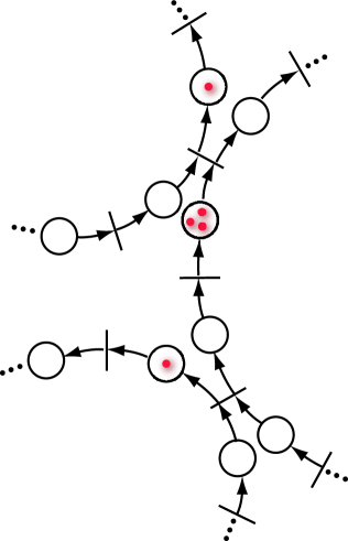
Figure 1: Petri Net Embodiment

Another motivating application comes from wireless sensor networks, where power management is important. A strategy for limiting power consumption is to limit the number of sensors that are on at any time, presumably selecting enough sensors to be on for adequate coverage of a field of interest, yet rotating which nodes deploy sensors over time, to extend lifetime and to improve robustness with regard to variation in sensor calibration. One solution to this problem would be to use clock synchronization, with a periodic schedule for sensing activity based on a global time. Alternatively, token circulation could be considered to activate sensors. Unlike a schedule purely based on synchronized clocks, a token-based solution provides some assurance and feedback in cases where nodes are faulty (e.g., when a token cannot be passed from one node to another due to a failure, such failure may be recognized and an alarm could be triggered). The abstraction of tokens put into messages may also allow aggregated sensor data or commands to be carried with a token, further enabling application behavior. Keeping tokens apart may relate to coverage goals for the sensor network: if tokens circulate in parallel and satisfy some distance constraint between them, then the sensors that are on at any time may provide adequate spatial diversity over the field of interest. Questions of satisfactory or optimal coverage of a field are beyond the scope of this paper. Our investigation is confined to the problem of self-stabilizing circulation of tokens with some desired separation between them.

Related Work.

Perhaps the earliest source on self-stabilization is [1], which briefly presents an algorithm to distribute $N$ points equally on a circle. The algorithm given in Section 6 distributes $m$ tokens equally around a ring, however the objective is a behavior (circulating tokens) rather than a final state. Papers on coordinated robot behavior, for example [2, 8, 3], are similar to [1] in that a geometric, physical domain is modeled. Most such papers consider a final robot configuration as the objective of distributed control and give the robots powerful vision and mobility primitives. Like the example of robot coordination, our work can have a physical control motivation, but we have a behavior as the objective. For results in this paper, the computation model is discrete and fully synchronous, where processes communicate only with neighbors in a ring. As for the sensor network motivation sketched above, duty-cycle scheduling while satisfying coverage has been implemented [4] (numerous network protocol and system issues are involved in this task [5]). These sensor network duty-cycle scheduling efforts are not self-stabilizing to our knowledge.

Within the literature of self-stabilization, a related problem is model transformation. If an algorithm $P$ is correct for serial execution, but not for a parallel execution, then one can implement a type of scheduler that only allows a process $p$ of $P$ to take a step provided that no neighbor $q$ is activated concurrently [6]; this type of scheduling is known to correctly emulate a serial order of execution. The problem we consider, separating tokens by some desired distance $d$, can be specialized to $d=2$ and be comparable to such a model transformation. For larger values of $d$, the nearest related work is the general stabilizing philosopher problem [7], which considers conflict graphs between non-neighboring philosophers. By equating philosopher activity (dining) to holding a token [7], we get a solution to the problem of ensuring tokens are at some desired distance, and also allowing tokens to move as needed. The synchronous token behavior in this paper differs from the philosopher problem because token circulation here is not demand-based; therefore solutions to the problem are obtained through the regular timing of token circulation.

Literature on self-stabilizing mutual exclusion includes token abstractions [10], generalizations of mutual exclusion to $k$-exclusion or $k$-out-of-$\ell$ exclusion [11], multitoken protocols for a ring [13], and group mutual exclusion [12]. Such literature does not constrain tokens to be separated by some desired distance $d$ (unlike the philosopher problem cited above), which differentiates our work from previous multitoken protocols. However, in applying the methods of this paper to some applications, it can be useful to employ self-stabilizing token or multitoken protocols at a lower layer: Section 5.2 expands on this idea of using self-stabilizing token protocols as a basis for our work.

The idea of using the timing of token arrival to control distributed behavior has previously investigated for balancing (or counting) networks, which can be seen as abstractions for scheduling. A token in a balancing network represents a locus of control; the path of a token over time describes the history of accesses that one process performs on distinct shared memory objects. States of the junctions in these networks change as tokens arrive and depart, and the state of a junction determines where an arriving token will be next routed. The relative timing of token arrivals to the network, and within the network, thus determine the pattern of flow through the network. Though such networks typically presume a properly initialized state, the idea of a self-stabilizing behavior in a balancing network has been proposed [16]. Balancing networks are generally open networks, where processes arrive, traverse the networks, and exit; presumably, the output of such a network could be fed back into the same network to make a closed system. Balancing networks are chiefly intended for asynchronous execution, where the objective is to obtain some pattern in the history of arrivals of processes to selected shared objects. Our goal is different: we suppose synchronous processes, with the time objective of keeping tokens some distance $d$ apart at all times. As an interesting aside, we note that algebraic (matrix) approaches have been found valuable both for Petri net analysis [9] and for combinatorial analysis of balancing networks [17].

If we move beyond guaranteed behavior in discrete-time models of circulating tokens to stochastic behavior of moving particles in large networks, then statistical physics literature on traffic may be relevant. Recent investigations consider capacity and efficiency metrics for flows of traffic [20], sometimes finding that separation between entities is important to shape traffic in the aggregate. Experiments have shown that the density of vehicles on a unidirectional circle cannot exceed a critical threshold without traffic jams appearing [19]; similar results appear to hold for complex networks, validated by simulation [21, 22].

2 Desired Behavior

Desired properties of a token circulation protocol are labeled as d1–d5 below.

d1 At any time, $m$ tokens are present in the system.

d2 The minimum distance between any two tokens is at least $d$.

d3 A token moves in each step from one process to a neighboring process.

d4 Every process has a token equally often; i.e., in an execution of $k$ steps, for any process $p_{i}$, there is a token at $p_{i}$ for approximately $k\cdot m/n$ steps.

d5 Following a transient failure that corrupts state variables of any number of processes, the system automatically recovers to behavior satisfying d1–d4.

In many topologies, not all of d1–d5 are achievable. As an instance, for d3 to hold, the center node of a star topology or a simple linear chain is necessarily visited by tokens more often than other nodes, conflicting with d4. The constructions of this paper are able to satisfy d1–d5 for a ring topology. Though it is straightforward to map a virtual ring on a complete walk over an arbitrary network, property d2 may not hold: nodes at distance $d$ in a virtual ring could be at much smaller distance in the base network. An example of a virtual ring is presented in Section 7.

3 Motivating Example

Though d4 cannot be achieved for a star topology in which tokens circulate the network, there is a simple case where separation of tokens can be obtained in an open network. Figure 2 shows how distance between tokens can be enforced almost trivially, by throttling the rate of tokens injected into the network.

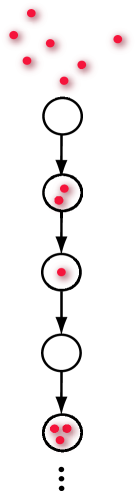
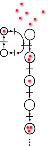
    Illustrated on the far left is an open system consisting of a chain of processes, $p_{1}$, $p_{2}$, …, with $p_{1}$ being the topmost process illustrated. Tokens are shown as dots, with a number of “loose tokens” above the chain representing new tokens arriving from outside the system to $p_{1}$. Each process $p_{i}$ releases at most one token in each round to $p_{i+1}$. The aim for this system is to ensure that, eventually, no two tokens are closer than some distance $d$ in the subchain from $p_{2}$ downward (we cannot prevent the accumulation of tokens are $p_{1}$ in this open system). On the immediate left is a simple delay mechanism shown as a Petri net; the small subring and the joint transition between $p_{1}$ and $p_{2}$ ensures that tokens do not arrive in each round to $p_{2}$. By adjusting the size of the subring, the target distance $d$ can be obtained.

Figure 2: Open System: Linear Chain

The delay mechanism between $p_{1}$ and $p_{2}$ is shown as a token ring conjoined to the chain. We use simpler notation for this later in the paper: a timer counts rounds between the times that tokens are released. If a new token arrives when the counter is zero, which is equivalent to a waiting token on the ring at the joint transition, then the new token is passed from $p_{1}$ to $p_{2}$ without additional waiting. The event of passing a token from $p_{1}$ restarts the timer; if a new token arrives with the counter is nonzero, then the new token will have to wait for the counter to reach zero before it can be released. This example reveals the strategy for separating tokens, namely to inject delay when needed. A question arising from Figure 2 is whether the same, simple idea can work in a closed system. What happens, for example, if the output from this chain, say at $p_{n}$, feeds back to $p_{1}$? Will this simple delay suffice for stabilization? Section 5 answers this question positively.

4 Notation and Model

Consider a ring of $n$ processes executing synchronously, in lock-step. Each process perpetually executes steps of a program, which are called local steps. In one global step, every process executes a local step. Programs are structured as infinite loops, where the body of a loop contains statements that correspond to local steps. We assume that all processes execute the loop steps in a coordinated manner: for processes running the same program, all of them execute the first statement step in unison. Similarly, if two processes run distinct programs, we suppose they begin the body of the loop together, which may entail padding the loop of one program to be the same number of steps as the other program. This assumption about coordination of steps is for convenience of presentation, since it is possible to engineer all programs to have a loop body with a single, more powerful step. The execution of all steps in the loop, from first to last statement, is called a round.

The notion of distance between locations in the ring can be measured in either clockwise or counterclockwise direction. In program descriptions and proof arguments, it is convenient to refer to the clockwise (counterclockwise) neighbor of a process using subscript notation: process $p_{i}$’s clockwise neighbor is $p_{i+1}$ and its counterclockwise neighbor is $p_{i-1}$. The distance from $p_{i}$ to itself is zero, the clockwise distance from $p_{i}$ to $p_{i+1}$ is one, and the counterclockwise distance from $p_{i}$ to $p_{i+1}$ is $n-1$; the counterclockwise distance from $p_{i}$ to $p_{i-1}$ is one, and general definitions of distance between $p_{i}$ and $p_{j}$ for arbitrary ring locations can be defined inductively. The counterclockwise neighbor of $p_{i}$ is called the predecessor of $p_{i}$, and the clockwise neighbor is called the successor.

The local state of a process $p_{i}$ is specified by giving values for its variables. The global state of the system is an assignment of local states for all processes. A protocol, specified by giving programs for each $p_{i}$, should satisfy the desiderata of Section 2. A protocol is self-stabilizing if, eventually, d1–d5 hold throughout the suffix of any execution. For simplicity, in the presentation of our protocols, we make some unusual model choices: in one case, $p_{i}$ assigns to a variable of $p_{i-1}$; and we assume that $m$ tokens are present in any initial state of any execution. After presenting programs in Section 5, we discuss in Subsection 5.2 these choices in reference to the two illustrative applications, Petri nets and sensor networks.

5 Protocol with Known Separation

This section presents a protocol to achieve and maintain a separation of at least $C+1$ links between tokens in the unidirectional ring. An implementation of the protocol uses four instantiation parameters, $n$, $m$, $C$, and the choice of which of two programs are used for nodes in the ring. Only the separation parameter $C$ is used in the protocol, as the domain of a counter, whereas the ring size $n$ and the number of tokens $m$ are unknown for the programs. The separation by $C+1$ links cannot be realized for arbitrary $n>1$ and $m>1$; we require that

$$m(C+1)\quad \leq \quad n$$ (1)

The protocol consists of two programs delay and relay. At least one process in the system executes the delay and any processes not running delay run the relay program. Processes running either program have two variables, $q$ and $r$; a process running delay has an additional variable $c$. To specify the variable of a particular process, we subscript variables, for instance, $q_{i}$ is the $q$ variable of process $p_{i}$. The domains of $q$ and $r$ are nonnegative integers; the domain of $c$ is the range of integers in $[0,C]$.

The $q$ and $r$ variables model the abstraction of tokens in a ring. At any global state $\sigma$, process $p_{i}$ said to have $t$ tokens if $r_{i}+q_{i}=t$. We say that $k$ tokens are resting at $p_{i}$ if $r_{i}=k$, and $\ell$ tokens are queued (for moving forward) if $q_{i}=\ell$. The objective of the protocol is to circulate $m$ tokens around the ring so that the distance from one token to the next (clockwise) token exceeds parameter $C$, and in each round every token moves from its current location to the successor. In some cases, it is handy to refer to the value of a variable at a particular state in an execution. The term $r_{i}^{\sigma}$ denotes the value of $r_{i}$ at a state $\sigma$. In most cases, the state is implicitly the present (current) state with respect to a description or a predicate definition.

Define the minimum clockwise distance between $p_{i}$ and a token to be the smallest clockwise distance from $p_{i}$ to $p_{j}$ such that $p_{j}$ has $t>0$ tokens. Observe that if $p_{i}$ has a token, then the minimum clockwise distance to a token is zero. Similarly, let the minimum counterclockwise distance from $p_{i}$ to a token be defined. Let $Rdist_{i}$ denote the minimum clockwise distance to a token for $p_{i}$ and let $Ldist_{i}$ denote the minimum counterclockwise distance to a token for $p_{i}$.

5.1 Programs

The delay and relay programs are shown in Figure 3. Both programs begin with steps to move any queued tokens from the predecessor’s queue to rest at $p_{i}$. The relay program enqueues one token, if there are any resting tokens, in line 3 of the program. The delay program may or may not enqueue a token, depending on values of the counter $c_{i}$ and the number of resting tokens $r_{i}$. In terms of a Petri net, the relay program corresponds to simple, deterministic, unit delay with at most one token firing in any step on the output transition. The delay program expresses a joint transition, with two inputs and two outputs: the variable $c_{i}$ becomes a ring of $C+1$ places and line 4 of delay represents the joint transition.

delay :: do forever 1 $r_{i}\;\leftarrow~{}r_{i}+q_{i-1}$  ; 2 $q_{i-1}\;\leftarrow~{}0$  ; 3 if  $c_{i}>0$  then $c_{i}\;\leftarrow~{}c_{i}-1$ 4 else if $c_{i}=0\;\wedge\;r_{i}>0$ then $c_{i}\;\leftarrow\;C$  ; $r_{i}\;\leftarrow\;r_{i}-1$  ; $q_{i}\;\leftarrow\;q_{i}+1$   relay :: do forever 1 $r_{i}\;\leftarrow~{}r_{i}+q_{i-1}$  ; 2 $q_{i-1}\;\leftarrow~{}0$  ; 3 if  $r_{i}>0$  then $r_{i}\;\leftarrow~{}r_{i}-1$  ; $q_{i}\;\leftarrow~{}q_{i}+1$

Figure 3: delay and relay programs

In application, it is possible that all $n$ processes run the delay program, and no process runs relay. This would be a uniform protocol to achieve d1–d5. An advantage of including relay processes can be to limit the cost of construction for physical embodiments of the logic. Using multiple relay processes can model more general cases of token delay: a consecutive sequence of $k$ relay processes is equivalent to a process that always delays an arriving token by $k$ rounds.

5.2 Application to Models

Petri Net.

It is usual for self-stabilization that transient faults, which inject variable corruption, are responsible for creating new initial states, and the event of a transient fault is not explicitly modeled. However for an application where tokens represent physical objects, which is plausible for Petri nets, a transient fault neither destroys nor creates objects. Thus we think it reasonable to suppose that $m>1$ tokens satisfying (1) are present in any initial state.

Observe that line 2 of either delay or relay has $p_{i}$ assign to $q_{i-1}$ (whereas the usual convention in the literature of self-stabilization is that a process may only assign to its own variables). The assignment $q_{i-1}\;\leftarrow\;0$ models the transfer of a token from a transition to its target place in a Petri net. For the firing of a Petri net transition, $p_{i}$ increments $q_{i}$ in line 4 of delay or line 3 or relay. Figure 1 illustrates both relay and delay programs. The portions of the two rings on the left side of the figure are modeled by the $c$ variables in relay nodes; these are “minor” rings with $C+1$ nodes, whereas the “major” ring has $n$ nodes. The situation of a token on a minor ring being ready for a transition shared by the major ring is modeled by $c_{i}=0$. Observe that when a token on the major ring is present at the same transition where a minor ring token exists, then transition firing is enabled at line 4, because $r_{i}>0$ and $c_{i}=0$. We assume that tokens of major and minor rings are of different nature; a transient fault cannot move a token from minor to major or from major to minor ring. A transient fault can move tokens arbitrarily on their respective rings.

Standard Models.

We first briefly review some conventions from the literature of self-stabilization. A typical model for self-stabilizing protocols is the shared variable model in which each process has access to some variables written by neighbor processes. In one atomic step, a process reads neighbor variables, performs some local computation, and writes to its variables. A system execution is a sequence of configurations, each configuration denoting the state of every process; between each consecutive pair of configurations in the execution there is a transition consisting of a some set of process steps (at most one step for each process). Standard models specify a scheduler, which selects, at each state in an execution, the process or processes that may take a step. The specification of the scheduler and the set of possible initial states is enough to generate all possible executions. Schedulers may be synchronous (all processes take a step in unison) or asynchronous; an extreme case of asynchrony is the central daemon scheduler, which selects just one process to take a step. The usual notation for programs is the guarded statement notation, wherein the program for each process is a set of guarded assignment statements. A guarded assignment is enabled at a particular state if the guard evaluates to true at that state. To avoid stuttering (repeated consecutive configurations in an execution), schedulers only select processes with enabled statements; also, programs are written so that any enabled statement should falsify its guard when executed (this is typically easy to verify for the central daemon scheduler). An execution is finite if its terminal state has no enabled statement, otherwise executions are infinite. Schedulers may have a number of choices of processes to select for the next step at a particular state. A fairness property of a scheduler is some policy to limits choices it makes over the course of an execution. An unfair scheduler has maximum freedom in the number and guard selection choice at any state. Experience has shown that programs are simplified when more assumptions can be made about the scheduler; for some problems, self-stabilization is not possible without the central daemon hypothesis of one process stepping in any state transition.

Considering how delay/relay may be fit to standard models, we see several obstacles: (i) $p_{i}$ assigns to $q_{i-1}$, which violates the rule of a process assigning to its own variables only; (ii) we have assumed that all process start their cycles together, which may not hold for an initial configuration; (iii) the number of tokens $m$ is supposed positive and constrained by (1) in the initial state; and (iv) execution is synchronous. Point (iv) is within the bounds of self-stabilization models, though one might hope for a realization of the same result for asynchronous models. Point (ii) will not be a concern if the programs delay and relay can each be reduced to a single guarded assignment; this is not a significant challenge, and we leave this as an exercise to the reader. We continue examining the other points in following paragraphs.

Regarding (i), there are two cases to consider, a synchronous or asynchronous execution model. In the case of synchronous execution, rewriting the program as a single guarded assignment can eliminate the assignment to $q_{i-1}$ in favor of having $p_{i}$ rewrite $q_{i}$, either to zero or to some new value if a token is queued. Because each process reads $q_{i-1}$ in each synchronous step, the logic of delay and relay is preserved by this rewriting. However, for an asynchronous model, some transformation is needed. For instance, a self-stabilizing protocol with acknowledgment [15] might be used to convey a token from $p_{i-1}$ to $p_{i}$ (note that this approach would entail bidirectional communication between $p_{i-1}$ and $p_{i}$). Alternatively, the task of passing a token from $p_{i-1}$ to $p_{i}$ could be handled by using a conventional self-stabilizing protocol, which we explain next under the discussion of point (iii).

Point (iii) raises the possibility that the initial state may not have $m>0$ tokens satisfying (1). Two ways to deal with this possibility are active monitoring and definitional approaches.

• The idea of active monitoring is to periodically sample the number of tokens and take appropriate measures for an incorrect value. Note that taking a sample is neither instantaneous nor reliable. A sample would need count the number of tokens that arrive to $p_{i}$, which should be $m$ tokens over $n$ time units when behavior is legitimate. This type of sampling is unreliable from an arbitrary initial state, because whatever variables are used for counting and measuring time are subject to transient fault corruption, hence false detection of an illegitimate state is possible. Moreover, if more than one process engages in sampling and correction, it could be that correction by one interferes with correction by another. The mechanism of distributed reset [14] might need to be employed for active monitoring and correction. In addition to the complexity of active monitoring, the potential for inserting and deleting tokens (perhaps unnecessarily) during convergence could be undesirable for the application using the tokens.

• The alternative to active monitoring is the definitional approach. Here, the system is built either from $m$ independent self-stabilizing token rings or from a self-stabilizing multitoken ring protocol that has $m$ tokens in a legitimate state. We sketch the case of $m$ independent token rings. For each token ring, there can be more than one token in an initial state. Provided that each process fairly includes steps from each of the $m$ token rings, each of these eventually converges to having a single token. A benefit of the definitional approach is that the token-passing mechanism is unidirectional: by writing to some variable designated for the token, the token is automatically available to the successor process.

Can the delay/relay protocol be extended to asynchronous scheduling? To reckon with (iv), some relaxation of d2-d3 is needed, because no mechanism in an asynchronous model can assure that two processes at distance $d$ release tokens simultaneously. A natural adaptation of the synchronous protocol is to leverage a self-stabilizing synchronizer, or a self-stabilizing phase clock.

A phase clock protocol equips each process $p_{i}$ with a clock variable $clock_{i}$. A clock has domain $[0,M]$, where $M$ has a lower bound related to the diameter of the network, but can otherwise be freely chosen; we suppose $M\bmod d=0$ for our design. The two crucial properties of a clock are (a) it increments modulo $M$ infinitely often in any execution, and (b) $|clock_{i}-clock_{j}|\leq 1$ for neighbors $i$ and $j$.

An adaptation based on a phase clock consists of allowing a cycle (translated into a guarded assignment) of delay/relay at $p_{i}$ to execute only when $clock_{i}\bmod d=0$ and the phase clock at $p_{i}$ is enabled to increment. The phases where $clock_{i}\bmod d=\ell$, for $\ell\in[1,d-1]$ are “idle” with respect to progress of delay/relay. Thus, $p_{i}$ can only release a token when $clock_{i}\bmod d=0$. Property (b) implies that a process $p_{k}$ at distance $d$ from $p_{i}$ satisfies $|clock_{i}-clock_{j}|\leq d$. Therefore, $clock_{k}$ could be “behind” $clock_{i}$ by $d$ phases when $p_{i}$ releases a token. Increments to the phase clock at $p_{i}$ continue during idle phases. The modulus $d$ provides sufficiently many idle phases to ensure that $p_{k}$ would release a token (provided it has one ready to release), before $p_{i}$ again encounters $clock_{i}\bmod d=0$.

Two difficulties need to be addressed in implementing this combining of delay/relay with a phase clock. First, we note that d2 can be violated in the combination, because $p_{i}$ may release a token before $p_{k}$ does, resulting in two tokens at distance $d-1$; some revision to $d$ or d2 is needed to handle this case. Another detail to cover in the adaptation is to prevent $p_{i+1}$ from immediately passing the token it receives from $p_{i}$, which would occur if $clock_{i+1}\bmod d=0$ upon reception. We omit further detail in this outline of adapting delay/relay to an asynchronous scheduler.

Wireless Sensor Network.

Wireless networks use messages rather than shared variables for communication. Several papers have proposed some implementation patterns for a shared variable model built upon sensor network abstractions. However, the definitional approach outlined above for tokens is well-suited to a message-passing architecture because releasing a token consists of a single write to a shared variable that is not again written until the next time a token is released. This allows the write to the shared variable to be replaced by a message transmission, from $p_{i}$ to $p_{i+1}$ (such a message would contain values for all $m$ independent token rings being emulated in the definitional construction).

Wireless sensors do have real-time clocks, though these may not be synchronized in an initial state. Therefore, a self-stabilizing clock synchronization protocol is warranted, so that the synchronous execution of delay/relay can be realized. With synchronized clocks, it is possible to define a recurring time interval so that all nodes start and end the execution of a delay/relay cycle together.

The preceding discussion assumes that messages are reliable. In practice, messages may be lost, which necessitates retransmission. The number of retransmits could be variable, which is problematic for defining intervals supporting synchronous execution of cycles. Of course, any protocol for wireless sensor networks faced with message loss is, at best, probabilistically valid.

5.3 Verification

A legitimate state for the protocol is a global state predicate, defining constraints on values for variables. To define this predicate, let $tokdist$ denote the minimum, taken over all $i$ such that $r_{i}+q_{i}>0$, of $Rdist_{i}$. The predicate $\textsf{delay}_{i}$ is true for process $p_{i}$ running delay and false for the relay processes.

Definition 1

A global state $\sigma$ is legitimate iff

$$\sum_{i}q_{i}=m \quad\wedge\quad \sum_{i}r_{i}=0\quad\wedge\quad(\forall i::\;q_{i}\leq 1)$$ (2)

$$\;\wedge\; tokdist>C$$ (3)

$$\;\wedge\; \left(\forall i:\;\textsf{delay}_{i}\;\wedge\;c_{i}>0\;\wedge\;q_{i}=0:\;Rdist_{i}=C-c_{i}\right)$$ (4)

$$\;\wedge\; \left(\forall i:\;\textsf{delay}_{i}\;\wedge\;q_{i}=0:\;Ldist_{i}>c_{i}\right)$$ (5)

$$\;\wedge\; \left(\forall i:\;\textsf{delay}_{i}\;\wedge\;q_{i}=1:\;c_{i}=C\right)$$ (6)

In an initial state, variables may have arbitrary values in their domains, subject to constraint (1).

Lemma 1 (Closure)

Starting from a legitimate state $\sigma$, the execution of a round results in a legitimate state $\sigma^{\prime}$.

• The conservation of tokens expressed by (2) is simple to verify from the statements of delay and relay programs, so we concentrate on showing that (3)–(6) are invariant properties. Assume that $\sigma$ is a legitimate state. We consider two cases for a process $p_{i}$ running delay, either there is no token at $p_{i}$ and $q_{i}=0$, or $q_{i}=1$ at $\sigma$.

  $\blacktriangleright q_{i}=1:$ observe that $c_{i}=C$ by (6). For $\sigma^{\prime}$ we have $r_{i}=0$ because from (3) there is no token at $p_{i-1}$ and we have $q_{i}=0\;\wedge\;c_{i}=C-1$ by lines 1-2 of either delay or relay at $p_{i+1}$, and line 3 of delay at $p_{i}$. This validates (2) with respect to the token passed, and (3) holds because every token moves to the successor starting from a legitimate state. Property (4) holds at $\sigma^{\prime}$ with respect to $p_{i}$ because $Rdist_{i}=1=C-c_{i}$. Finally, (5) is validated for $p_{i}$ because, if (5) holds for $\sigma$ when $c_{i}=C$, then a token moving one process closer to $p_{i}$ validates (5) by $c_{i}=C-1$ at $\sigma^{\prime}$.

  $\blacktriangleright q_{i}=0:$ there are two subcases, either $c_{i}=0$ or $c_{i}>0$. In the former case, if no token arrives to $p_{i}$ in the transition from $\sigma$ to $\sigma^{\prime}$, properties (2)-(6) directly hold with respect to $p_{i}$ in $\sigma^{\prime}$. If a token arrives to $p_{i}$, then $q_{i}=1\;\wedge\;c_{i}=C$ result by line 4 of delay, and we use properties (3)-(6) of $p_{i-1}$ at $\sigma$ to infer that the same properties hold of $p_{i}$ at $\sigma^{\prime}$. If $c_{i}>0$ at $\sigma$, then by (3)-(5) and legitimacy of all processes within distance $C+1$ in either direction from $p_{i}$, tokens move to the successor process while $c_{i}$ decrements, which establishes (3)-(5) for $p_{i}$ at $\sigma^{\prime}$.      

To prove convergence, we start with some elementary claims and define some useful terms. Suppose rounds are numbered in an execution, round $t$ starts from state $\sigma$, and that $q_{i-1}^{\sigma}=v$. For such a situation, we say that $v$ tokens arrive at $p_{i}$ in round $t$.

Claim 1

In any execution, $\sum_{i}r_{i}+q_{i}\;=\;m$ holds invariantly.

• As explained in Section 4, $m>1$ tokens are present in the initial state, represented by $r_{i}$ and $q_{i}$ variables. Statements of delay or of relay conserve the number of tokens in the system, because we assume that all processes execute lines 1 and 2 synchronously in any round. Line 4 of delay or line 3 of relay similarly conserve the number of tokens in a process.      

Claim 2

Within one round of any execution,

$$(\;\forall\,i::\quad q_{i}\leq 1\;)$$ (7)

holds and continues to hold invariantly for all subsequent rounds.

• In every round, line 2 of delay or relay assigns $q_{i-1}\leftarrow 0$, and may assign $q_{i}\leftarrow 1$.      

For the remainder of this section, we consider only executions that start with a state satisfying (7). For such executions, a corollary of Claim 2 is: at most one token arrives to any process in any round.

Claim 3

If $m>0$, then for every execution of the protocol and $0\leq k<C\;\wedge\;0\leq i<n$, the variable $c_{i}=k$ at infinitely many states.

• The proof is by contradiction. First, we show that at least some token moves infinitely often. Since $m>0$, there is a token at some process $p_{i}$ because $r_{i}>0$ or $q_{i}>0$; the case $q_{i}>0$ implies immediate token movement in the next round, so we look at the other case, $r_{i}>0\;\wedge\;q_{i}=0$. In one round, $p_{i}$ either assigns $q_{i}\leftarrow 1$ program, and thus a token moves in the next round, or $p_{i}$ assigns $c_{i}\leftarrow c_{i}-1$ because $c_{i}>0$. Therefore, after at most $C$ rounds, a state where $c_{i}=0\;\wedge\;r_{i}>0$ is reached, and the next round enqueues a token for movement. The preceding argument shows that some token movement occurs infinitely often in any execution. There are $m$ tokens throughout the execution by (2), hence at least one token can be considered to move infinitely many times. Note that the token abstraction is represented by $r$ and $q$ variables only: we cannot be sure that one token does not overtake another token. However, it will be our convention to model token queuing as first-in, first-out order. Thereby we find that if one token moves infinitely many times clockwise around the ring, all tokens do so as well. Returning to the claim, suppose that some $c_{i}$ variable eventually never has some value $k\in[0,C-1]$. But $p_{i}$ experiences infinitely many tokens arriving and assigns $q_{i}\leftarrow 1$ infinitely often, so lines 3 and 4 of delay execute infinitely often at $p_{i}$, which is a contradiction.      

Claim 4

For any process $p_{i}$ running the delay program, eventually $p_{i}$ assigns $q_{i}\leftarrow 1$ at most once in any $C+1$ consecutive rounds.

• Claim 3 shows that $p_{i}$ eventually assigns $c_{i}\leftarrow C$. In delay, only line 4 assigns $q_{i}\leftarrow 1$, and the same step assigns $c_{i}\leftarrow C$. Thus, if we number rounds $t$, $t+1$, and so on, the values of $c_{i}$ and $q_{i}$ variables at the end of each round is shown by:

  round	$t$	$t+1$	$t+2$	$\cdots$	$t+(C-1)$	$t+C$	$t+(C+1)$
  $c_{i}$	$C$	$C-1$	$C-2$	$\cdots$	1	0	$C$
  $q_{i}$	1	0	0	$\cdots$	0	0	1

The table makes the worst-case assumption that $r_{i}>0$ at round $t+(C+1)$, to illustrate that through at least $C$ consecutive rounds, $q_{i}$ remains zero.      

Claim 5

Let $\sigma$ be a state that occurs after sufficiently many rounds so that every token has arrived at least once at some process running the delay program. In the (suffix) execution following $\sigma$, if a token arrives at $p_{i}$ in round $t$, then no token arrives at $p_{i}$ during rounds $t+1$ through $t+C$.

• After $\sigma$, a token departs from any given delay process $p_{i}$ only at line 4 of delay, which has precondition $c_{i}=0$ and postcondition $c_{i}=C$. Thus, each delay process releases a token once every $C+1$ rounds (or less often, if $r_{i}=0$ holds). A relay process $p_{j}$ could potentially release tokens once per round, if $r_{j}$ remains positive, however we have supposed that each token has entered some delay process before $\sigma$. A simple inductive argument shows that $r_{j}=0$ holds throughout the execution following $\sigma$. Therefore, each process experiences token arrival at most once every $C+1$ rounds.      

Below we consider only executions that start with a state $\sigma$ satisfying (5). For such executions, a corollary of Claim 5 is: the token arrival rate to any process is at most $1/(C+1)$.

Claim 6

Let $\sigma$ be a state in any execution identified by Claim 5. Then, throughout the remainder of the execution,

$$(\;\forall\,i::\quad r_{i}\leq 1+r_{i}^{\sigma}\;)$$ (8)

• If some $r_{i}$ increases in a round, then because of Claim 5, no additional token arrives to $p_{i}$ for $C+1$ rounds; this is an adequate number of rounds to ensure that $p_{i}$ will release a token, thus putting $r_{i}$ back to its original value.      

Claim 6 allows us to introduce the notion of a resting bound for any process $p_{i}$. With respect an execution $E$ with an initial state $\sigma$ as defined in Claim 5, for each $p_{i}$ executing the delay program there is a bound $1+r_{i}^{\sigma}$ on the number of tokens that may rest together at $p_{i}$ during the remainder of $E$. After any round in $E$ producing a state $\beta$, let us consider three possibilities for any particular delay process $p_{i}$’s number of resting tokens:

$$r_{i}^{\beta}=(1+r_{i}^{\sigma})\quad\vee\quad r_{i}^{\beta}=r_{i}^{\sigma}\quad\vee\quad r_{i}^{\beta}<r_{i}^{\sigma}$$

Notice that for the first two disjuncts, the resting bound of $r_{i}$ is unchanged. However, for the third disjunct, where $p_{i}$ released a token in the round and has fewer than $r_{i}^{\sigma}$ resting tokens, the argument of Claim 6 can be applied to state $\beta$, lowering the resting bound for $p_{i}$ to $1+r_{i}^{\beta}$. More generally, there might be other processes that lower their resting bounds during the round obtaining $\beta$. Thus, the resting bound developed by Claim 6 for each process may improve during an execution. At any particular point in $E$, the best bound for $r_{i}$ is $1+r_{i}^{\delta}$, where $\delta$ is determined by the most recent round that lowered $r_{i}$’s resting bound; if there is no such preceding round, then let $\delta=\sigma$. Below, we find special cases with more accurate bounds.

Resting bounds are the basis for a variant function on protocol execution. Let $F$ be a tuple formed by listing the resting bounds for all delay processes. Since no process increases its resting bound in any round, it follows that valuations of $F$ can only decrease during execution. If all components of tuple $F$ are zero, then it is possible to show that the protocol has reached a legitimate state. We say that $F$ is positive if any of its components is nonzero. In order to prove convergence, two more claims are needed. First, a special case is required for a resting bound of zero (since Claim 6’s form is inappropriate); second, it must be shown that $F$ eventually does decrease if it is positive.

Claim 7

Let $E$ be an execution originating from a state $\sigma$ identified by Claim 5, and suppose $\alpha$ is a state in $E$ where $p_{i}$ running delay satisfies $r_{i}^{\alpha}=0\;\wedge\;c_{i}^{\alpha}=0$. Then, for the execution following $\alpha$, the resting bound of $r_{i}$ is zero.

• The proof is by induction over the execution following $\alpha$, based on the sequence of rounds associated with token arrival at $p_{i}$. When a token arrives at $p_{i}$ after state $\alpha$, the predicate $r_{i}=0\;\wedge\;c_{i}=0$ holds. The delay program establishes $q_{i}=1\;\wedge\;r_{i}=0\;\wedge\;c_{i}=C$ when processing the arriving token. Claim 5 ensures that no additional token will arrive to $p_{i}$ during the following $C$ rounds, so that $c_{i}=0$ holds when the next token arrival occurs for $p_{i}$.      

Claim 8

Let $E$ be an execution originating from a state $\sigma$ identified by Claim 5. $F$ cannot be positive and constant throughout $E$.

• Proof by contradiction. Suppose, for each delay $p_{i}$, that the resting bound never decreases. We analyze scenarios for this supposition and derive necessary conditions, which are used to show a contradiction. Claim 3 implies that $p_{i}$ receives a token infinitely often in $E$ and releases a token infinitely many times. If each token reception coincides with releasing a token, which entails $c_{i}=0$, then $r_{i}>0$ would remain constant throughout $E$. For such a continuing scenario, $p_{i}$ must receive at token once every $C+1$ rounds. The other possible scenario is that of $r_{i}$ incrementing to the resting bound, then decrementing, and repeating this pattern. For this scenario, $c_{i}$ decrements to zero, then resets to $C$, continuously during $E$. Because we have supposed that $r_{i}$ never decrements twice before incrementing again (otherwise $F$ would decrease), tokens need to arrive sufficiently often to $p_{i}$. Suppose $c_{i}=k>0$ when a token arrives. Then another token must arrive after exactly $C+1$ rounds so that $c_{i}=k$ upon token arrival. If instead, a token arrives after $C+1+d$ rounds, then $c_{i}=k-d$ would hold upon token arrival, $d\leq k$. More generally, the spacing in token arrivals over $E$ could be $C+1+t_{1}$, then $C+1+t_{2}$, and so on up to a delay gap of $C+1+t_{\ell}$ rounds, so long as $\sum_{j=1}^{\ell}t_{j}\leq k$. Each time there is a delay gap of $C+1+t_{j}$ rounds with $t_{j}>0$, the counter $c_{i}$ decreases in this scenario. A decrease resulting in $c_{i}=0$ would then force all future delays to be $C+1$, so that tokens arrive exactly as they are released, preventing a reduction of $r_{i}$.

  Having exposed the scenarios for $F$ remaining constant over execution $E$, thus at least one $r_{i}>0$ throughout $E$, we observe that from $m(C+1)\leq n$ there exists a segment of the ring, with more than $C+1$ processes, containing no token, at every state in $E$. The existence of such a segment implies that some delay $p_{i}$ will receive a token after a delay of more than $C+1$ rounds (a more detailed argument could take into account processes identified by Claim 7, which merely pass along tokens when they arrive). Thus, infinitely often, a delay between token arrivals is at least $C+2$ rounds. It follows that eventually, $c_{i}$ decreases to zero for some $p_{i}$ before a token arrives, at which point it will decrease $r_{i}$, contradicting the assumption that $F$ remains constant.      

Lemma 2 (Convergence)

Every execution of the protocol eventually contains a legitimate state.

• The proof is by induction on Claim 8, so long as $F$ is positive. Therefore, the resting bound for every delay process is zero eventually. To establish that the resulting state is legitimate, it is enough to verify the behavior of a delay process $p_{i}$ during the $C+1$ rounds preceding token arrival to see that (3)-(5) hold with respect to $p_{i}$.      

We sketch an argument bounding the worst-case convergence time using elements from the proof of convergence. The variant function $F$ is applied to an execution suffix satisfying (7), and Claim 5; such a suffix occurs within $O(n)$ rounds of any execution: the worst case occurs when one delay process $p_{i}$ holds all $m$ tokens, which it releases after at most $m\cdot C$ rounds, and the last of these tokens takes $O(n)$ rounds to again arrive at a delay process; since $m\cdot C\leq n$ by (1), we have $O(n)$ rounds overall to obtain the suffix for Claim 5. To bound the worst case for $F$ reducing in an execution, we observe that there are at most $n$ components to $F$, each with an initial maximum value of $m$. Suppose each component decreases sequentially, therefore requiring $n\cdot m\cdot f$ time, where $f$ is the worst-case number of rounds to reduce one component of $F$. We bound $f$ by the proof argument of Claim 8. A ring segment of length at least $C+2$ and devoid of tokens implies some decrease of a resting bound in the proof argument. This decrease may take $O(C)$ time to occur, as a $c$ variable reduces while a process awaits a token. If $f\in O(C)$, an overall bound on convergence time is $O(n)+O(n\cdot m\cdot C)=O(n^{2})$; however, if the ring segment without tokens is longer, then a delay process may spend more time awaiting a token. A conservative bound is therefore $O(m\cdot n^{2})=O(n^{3})$ rounds.

As an aside, we note that the algorithms are deterministic, execution is fully synchronous (there is no nondeterministic adversary), and the program model fits the Petri net formalism; therefore a formulation using the max-plus algebra [9] can express system execution, and there exist tools to compute eigenvalues for a matrix representing the system. We did not investigate such an approach, since the choice of which processes run delay would be an extra complication.

Each point is derived from 300 simulations with a random initial state and random selection of which processes run delay, ranging from one to 50 on the $x$-axis; the $y$-axis is the average number of rounds for convergence.

Figure 4: Simulations with $n=50$, $m=2$ and $m=5$

The graph on the left continues the type of simulation shown in Figure 4, however with 10 tokens. The graph on the right varies the ring size, $n=10i$ for $0<i<20$, in each case letting $m=2$, $d=\lfloor n/3\rfloor$, and the number of delay processes be $n/2$.

Figure 5: Other simulations

We have simulated the protocol for various cases of $n$, $m$, $C$, and choices for the number of delay processes. These simulations suggest that a bound $O(n^{3})$ may be loose for the average case. Another point of the simulation is to investigate the influence of having multiple delay processes on convergence time. Our simulations explored random initial values for variables. Three graphs, spread over figures 4 and 5, experiment with differing values of $m$ and $d$, all for a 50-node ring. In each graph, an experiment is repeated for different numbers of delay processes, from 1 to 50. The results suggest that having at least a few delay processes is beneficial. To explore another dimension, the ring size $n$, a fourth graph presented in Figure 5 varies $n$: the results suggest that expected convergence time is linear in $n$.

Theorem 1

The delay/relay protocol, with at least one delay process, and with $n>1$, $m>1$, $d=C+1$, and $m\cdot d\leq n$, self-stabilizes to desiderata d1-d5.

• Claim 1 attends to d1, The definition of legitimate state validates d2. A property of a legitimate state is that $c_{i}=0$ whenever a token arrives to $p_{i}$, hence the behavior of delay is like relay: a token moves in each round, as required by d3. The ring topology and the unidirectional movement of tokens satisfies d4. Finally, lemmas 2 and 1 provide the technical basis for the theorem, showing d5.      

6 Protocol with Unknown Ring Size

A parameter $C$, upon which the target separation between tokens is based, is given to the protocol of Section 5. Here we consider another design alternative, where the separation between tokens should be maximized, but the ring size is unknown. The technique is straightforward: building upon the delay program, additional variables are added to count the number of rounds needed to circulate a token, that is, the new program calculates $n$. Two extra assumptions are used for the new protocol: the value of $m$ is known and the number of processes running the delay program is exactly one. We discuss this limitation in Section 7.

delay :: do forever 1 $t_{i}\;\leftarrow\;t_{i}+1$  ; 2 if $q_{i-1}>0\;\wedge\;timing_{i}$ then 3 $ignore_{i}\;\leftarrow~{}ignore_{i}-1$  ; 4 if  $ignore_{i}<1$  then 5 $timing_{i}\;\leftarrow~{}\textit{false}$ ; 6 $ClockBase_{i}\;\leftarrow~{}\lfloor t_{i}/M\rfloor-1$ 7 $r_{i}\;\leftarrow~{}r_{i}+q_{i-1}$  ; 8 $q_{i-1}\;\leftarrow~{}0$  ; 9 if  $c_{i}>0$  then 10 $c_{i}\;\leftarrow~{}c_{i}-1$ 11 else if $c_{i}=0\;\wedge\;r_{i}>0$ then 12 $c_{i}\;\leftarrow\;ClockBase_{i}$  ; 13 $r_{i}\;\leftarrow\;r_{i}-1$  ; 14 $q_{i}\;\leftarrow\;q_{i}+1$  ; 15 if $\neg timing_{i}$ then 16 $timing_{i}\;\leftarrow\;\textit{true}$  ; 17 $t_{i}\;\leftarrow\;0$  ; 18 $ignore_{i}\;\leftarrow\;M-r_{i}-1$

Figure 6: delay program revised to calculate ring size

Figure 6 presents the revised delay program, which introduces $timing_{i}$, $t_{i}$, $ignore_{i}$, and $ClockBase_{i}$. The program uses $ClockBase_{i}$ in place of parameter $C$, which is periodically recalculated. The method of calculation relies upon knowing $M$ and knowing that all other processes run relay. The program begins a timing phase in lines 16-18, which starts a counter $t_{i}$ at zero, and calculates the number of tokens that are elsewhere in the ring, $ignore_{i}$. Subsequently, lines 3-6 handle token arrival for purposes of calculating ring size; after $ignore_{i}$ arriving tokens are ignored, the next token is the one that was released when the timing phase began. Of course, this calculation can be incorrect in early rounds of an execution, but eventually each timing phase culminates in $t_{i}$ having the ring size at line 6.

Lemma 3

With the delay program of Figure 6 at one process and relay at all other processes, the system is self-stabilizing to $C=\lfloor n/m\rfloor-1$.

• By arguments below, in any execution, $ClockBase_{i}=\lfloor n/m\rfloor-1$ holds throughout a suffix execution. Lemmas 1 and 2 then apply to verify self-stabilization.

  Let $p_{k}$ be the sole delay process. For convergence, it is enough to show that $ClockBase_{k}$ obtains the maximum feasible value for $m$ tokens, that is, $ClockBase_{k}=\lfloor n/m\rfloor-1$ holds throughout a suffix of any execution. The proof hinges on two cases, either (1) we have $(\forall i:\;i\neq k:\;r_{i}=0)$, or (2) some tokens rest at relay processes. In case (1), because $p_{k}$ releases at most one token per round, and because all relay processes pass along the token it receives in the next round, it follows that (1) holds invariantly. Provided $m>0$, process $p_{k}$ infinitely often receives and releases a token in any execution, so lines 5-6 and lines 16-18 of Figure 6 are executed repeatedly. Line 18 calculates one fewer than the number of tokens that do not rest at $p_{k}$ at the instant a token is released from $p_{k}$ to $p_{k+1}$. Provided (1) holds, it will be $n$ subsequent rounds before this token circulates the ring and returns to $p_{k}$. Lines 1-6 compute the elapsed time between the release of this token and its return, so that $t_{k}=n$ when line 6 calculates the value of $ClockBase_{k}$, and this drives convergence in the remainder of the execution. Case (2) eventually disappears, because $ClockBase_{k}>1$ is calculated in each execution of line 6. Resting tokens for relay processes therefore do not persist, assuming $m<n$: no process receives a new token in every round, hence any positive number of resting tokens reduces to zero, from whence the count of resting tokens cannot rise.      

7 Discussion

This paper provides fault tolerant constructions for a timing behavior in which $m$ loci of control are separated. The program mechanisms are simple: tokens carry no data and processes use few variables. The first construction can be uniform, distinguished (with one unique corrective process), or hybrid. The second construction requires one distinguished process.

An interesting question is whether there can be a hybrid or uniform protocol when the ring size and separation constant are unknown. For the style of algorithm in Section 6 we conjecture the answer is negative. If one delay process $p_{i}$ has an accurate estimate for maximum separation $d=c_{i}+1$ and does not delay any arriving token, another process $p_{j}$ may have either a larger, inaccurate estimate, or may perceive that tokens are unaligned with its counter and therefore delay some arriving tokens. Such delay would lead to $p_{i}$ detecting an apparently larger ring size, since the measured traversal time around the ring would include $p_{j}$’s delays. Hence $p_{i}$ would raise its estimate for the separation value. Note that the problem may admit other types of algorithms: for example, if tokens are allowed to carry data, this would enable processes to communicate. Whether such increased communication power is useful is an open question. Another direction would be to use randomized timing, so that different delay processes do not interfere.

The program of Section 5 conforms to the standard Petri net model of behavior control if we replace counters by auxiliary token rings, as shown in Figure 1. This restriction enables tokens to model a physical system. However, programs that use tokens to carry data and thus communicate with explicit data rather than mere timing of tokens would need more functionality from a physical embodiment than Section 5’s programs use in their timing-only mechanism. We have preferred for the present to investigate algorithms that use only the timing of tokens to overcome an unpredictable initial state.

An obvious direction for future research is to move beyond rings to other topologies. We think it likely that some of the desiderata d1–d5 will be relaxed for other topologies. Figure 7 suggests how a virtual ring, induced by a walk that includes all nodes, might be mapped upon a network. Our protocols could be adapted to run on the virtual ring, and this might provide separated token circulation. Note that distance between tokens in the virtual ring could map to smaller distance in the underlying topology, because a node may appear more than once in the virtual ring. The existence of a walk for which $m$ tokens can be separated by distance $d$ in the underlying topology is an open question. Instead of mapping a complete walk of the network nodes, another strategy could be to map distinct rings upon a network so that they cover all nodes, and then hope to coordinate the timing of token circulation in these rings where they intersect.

A complete walk of the network shown induces a virtual ring; nodes in the center row of the network occur more than once in the walk, conflicting with d4. Shown are three tokens separated by distance at least two; as all tokens synchronously follow the walk, the separation by $d=2$ persists in the underlying network.

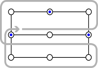
Figure 7: Virtual Ring

References

- [1] EW Dijkstra. EWD386 The solution to a cyclic relaxation problem. In Selected Writings on Computing: A Personal Perspective, pp. 34-35, Springer-Verlag, 1982.
- [2] Y Asahiro, S Fujita, I Suzuki, M Yamashita. A Self-stabilizing Marching Algorithm for a Group of Oblivious Robots. In OPODIS 2008, pp. 125-144, Springer LNCS 5401, 2008.
- [3] M Cieliebak, P Flocchini, G Prencipe, N Santoro. Solving the Robots Gathering Problem. In ICALP 2003, pp. 1181-1196, Springer LNCS 2719, 2003.
- [4] T He, S Krishnamurthy, L Luo, T Yan, L Gu, R Stoleru, G Zhou, Q Cao, P Vicaire, JA Stankovic, TF Abdelzaher, J Hui, B Krogh. VigilNet: An Integrated Sensor Network System for Energy-Efficient Surveillance. ACM Transactions on Sensor Networks 2 1:1-38, 2006.
- [5] L Wang, Y Xiao. A Survey of Energy-Efficient Scheduling Mechanisms in Sensor Networks Mobile Networks and Applications 11, 5:723-740, 2006.
- [6] MG Gouda, F Faddix. The Alternator. In WSS 1999, pp. 48-53, 1999.
- [7] P Danturi, M Nesterenko, S Tixeuil. Self-stabilizing Philosophers with Generic Conflicts. In SSS 2006, pp. 214-230, Springer LNCS 4280, 2006.
- [8] P Flocchini, G Prencipe, N Santoro. Self-Deployment of Mobile Sensors on a Ring. Theoretical Computer Science 402(1):67-80, 2008.
- [9] F Baccelli, G Cohen, GJ Olsder, JP Quadrat. Synchronization and Linearity: An Algebra for Discrete Event Systems. Wiley, 1992.
- [10] S Dolev. Self-Stabilization, MIT Press, 2000.
- [11] AK Datta, R Hadid, V Villain. A New Self-Stabilizing -out-of- Exclusion Algorithm on Rings. In SSS 2003, pp. 113-128, Springer LNCS 2704, 2003.
- [12] S Cantarell, F Petit. Self-Stabilizing Group Mutual Exclusion for Asynchronous Rings, In OPODIS 2000, pp. 71-90, 2000.
- [13] M Flatebo, AK Datta, AA Schoone. Self-Stabilizing Multi-Token Rings, Distributed Computing 8(3):133-142, 1995.
- [14] A Arora, MG Gouda. Distributed Reset. IEEE Trans. Comput. 43(9):1026-1038, 1994.
- [15] Y Afek, GM Brown. Self-Stabilization of the Alternating-Bit Protocol. Distributed Computing, 7:27-34, 1993.
- [16] M Herlihy, S Trithapura. Self-stabilizing Smoothing and Counting. In 23rd IEEE International Conference on Distributed Computing Systems ICDCS 2003, pp. 4-11, 2003.
- [17] C Busch, M Mavronicolas. A Combinatorial Treatment of Balancing Networks. Journal of the ACM 43(5):794-839, 1996.
- [18] T Herman, K Ghosh Dastidar. Separation of Circulating Tokens. In SSS 2009, pp. 354-368, Springer LNCS 5873, 2009.
- [19] Traffic Jams Without Bottlenecks. Y Sugiyama, M Fukui, M Kikuchi, K Hasebe, A Nakayama, K Nishinari, S Tadaki, S Yukawa. New Journal of Physics 10:033001, 2008.
- [20] D Helbing. Traffic and Related Self-Driven Many-Particle Systems. Rev. Mod. Phys. 73:1067-1141, 2001.
- [21] P Holme. Congestion and Centrality in Traffic Flow on Complex Networks, 2003. http://arxiv.org/abs/cond-mat/0301013.
- [22] L Zhao, Y-C Lai, K Park, N Ye. Onset of Traffic Congestion in Complex Networks. Phys. Rev. E 71(2):026125, 2005.