Dust-Dust Collisional Charging and Lightning in Protoplanetary Discs

Abstract

We study the role of dust-dust collisional charging in protoplanetary discs. We show that dust-dust collisional charging becomes an important process in determining the charge state of dust and gas, if there is dust enhancement and/or dust is fluffy, so that dust surface area per disc volume is locally increased.

We solve the charge equilibrium equations for various disc environments and dust number density $\eta$, using general purpose graphic processors (GPGPU) and cuda programming language. We found that as dust number density $\eta$ increases, the charge distribution experience four phases. In one of these phases the electrostatic field $E$ caused by dust motion increases as $E\propto\eta^{4}$. As a result, macroscopic electric discharge takes place, for example at $\eta=70$ (in units of minimum-mass solar nebula (MMSN) values, considering two groups of fluffy dust with radii $10^{-2}\ \mathrm{cm}$, $10^{2}\ \mathrm{cm}$). We present a model that describes the charge exchange processes in the discs as an electric circuit. We derive analytical formulae of critical dust number density for lightning, as functions of dust parameters.

We estimate the total energy, intensity and event ratio of such discharges (‘lightning’). We discuss the possibility of observing lightning and sprite discharges in protoplanetary discs by Astronomically Low Frequency (ALF) waves, IR images, UV lines, and high energy gamma rays. We also discuss the effects of lightning on chondrule heating, planetesimal growth and magnetorotational instability of the disc.

1 Introduction

Planets are formed in protoplanetary discs from interstellar dust. The electric charge state of the dust aggregates in the protoplanetary discs is one of the key parameters in understanding a number of aspects of protoplanetary discs and protoplanetary formation.

Planet formation begins with mutual sticking of$\ \mathrm{\mu m}$-sized dust, most probably leading to extremely low density, fluffy structure of the dust (e.g. Ossenkopf, 1993). The occurrence of fluffy dust is suggested by laboratory experiments (e.g. Wurm & Blum, 1998; Blum et al., 1998), by theories (e.g. Ormel et al., 2007; Zsom & Dullemond, 2008), by N-body simulations (e.g. Kempf et al., 1999; Suyama et al., 2008; Wada et al., 2008a), and by observations, including optical observations of dust in star forming region (e.g. Evans et al., 2001) and observations of dust linear polarization in comet comae (Levasseur-Regourd et al., 2007). For a review of this field, see e.g. Blum (2004).

The inner structure of the dust aggregates, relative velocity, and electric charge are key parameters that determine the growth and migration of dust aggregates. Dust relative velocity (Brauer et al., 2008) includes random motion caused by turbulence (Ormel & Cuzzi, 2007) and Brownian motion (Blum et al., 1996), and bulk motion caused by vertical sedimentation (Dullemond & Dominik, 2004) and radial migration (Weidenschilling, 1977). The collision velocity governs the growth rate (Suyama et al., 2008), compactification (Weidling et al., 2009), and disruption (Wada et al., 2008a), of the dust.

Okuzumi (2009) considered the charge state of the dust aggregates in protoplanetary discs. They assumed that the charge state is determined by absorption equilibrium of ions and free electrons. Since electrons have much larger thermal velocity compared to positive ions, plasma absorption makes all dust to charge weakly negative. The repulsive Coulomb force may suppress dust-dust collisional growth for all but the heaviest dust species who can overcome the Coulomb barrier.

It is also possible that the charge state of the dust is affected by dust-dust collision. The effect has been simply ignored in most research due to the fact that in protoplanetary discs, dust has low number density, and is surrounded by weakly ionised plasma. We give quantitative estimates of the effect of dust-dust collision as a function of dust size, fractal dimension, and number density, and show for the first time that the dust-dust collision is actually an important factor in high dust number density regions of protoplanetary discs.

One of the possible dust-dust collisional charging mechanisms is known as the triboelectric process, where two bodies exchange electrons and sometimes molecular ions when they come into contact (e.g. Sickafoose et al., 2001). Another mechanism is possible for materials with spontaneous surface charge, such as $\mathrm{H_{2}O}$ ice crystals (e.g. Kudin & Car, 2008). In this mechanism the surface matter within typical depth $\sim 1.0\times{10}^{-4}\ \mathrm{cm}$ (Mason & Dash, 2000) is exchanged together with contained charge.

Surface space charge due to electron spill-out is widely known among metals and semiconductors (Somorjai, 1994), the charge separation being $\sim 10^{-7}\ \mathrm{cm}$ deep for metals and $\sim 10^{-5}\ \mathrm{cm}$ deep for semiconductors. $\mathrm{H_{2}O}$ is unique in that molecular ions $\mathrm{OH^{-}}$ and $\mathrm{H_{3}O^{+}}$ holds the charge, and that proton exchange between the molecules (Grotthus mechanism; c.f. Agmon, 1995) allows charge diffusion much faster than molecular ion diffusion. Thus surface charge separation develops as deep as $\sim 2.0\times{10}^{-4}\ \mathrm{cm}$ (Dash et al., 2001). For example, ammonia lacks the mechanism (Goncalves et al., 1999). It is important that charge separation layer is deeper than exchange depth, because if the entire charge separation layer is exchanged, charge transport is neutral and collisional charging do not take place.

The dust-dust collisional charging due to the exchange of this spontaneous surface charge of ice crystals, is an established model in the context of meteorology (e.g. Takahashi, 1978; Baker et al., 1987; Dash et al., 2001) that explains lightning on earth. When two ice dust of different surface states collide, they exchange their surface charge, producing charged dust. When the charged particles within nonconducting gas are separated by some external force, electric field grows between them. At the point the electric field is larger than the dielectric field strength of the gas, rapid ionisation of the gas occurs, converting the electrostatic energy into kinetic energy of the electrons and ions. This is electric discharge. Lightning in the earth’s atmosphere is one of the most prominent, and well studied examples of electric discharge phenomena; in thunderclouds, typically $3.0\times{10}^{10}\ \mathrm{esu}$, or $1.0\times{10}^{1}\ \mathrm{C}$ of electric charge is repeatedly separated and neutralized with typical length scales $1.0\times{10}^{5}\ \mathrm{cm}$ (Koshak & Krider, 1989).

In protoplanetary discs, lightning is one of the candidate mechanisms for chondrule heating, although compared to other models e.g. heating by shock wave (e.g. Miura et al., 2008), some difficulties have been pointed out (Weidnschilling, 1997). For example, electric field cannot grow large enough to cause electrostatic breakdown in standard discs (Gibbard et al., 1997). Moreover, when$\ \mathrm{mm}$-sized silicate aggregates made of$\ \mathrm{\mu m}$-sized monomers are subject to electric discharge, they generally fragment without being thermally processed (Güttler et al., 2008).

Lightning in protoplanetary discs is strongly related to turbulence. The relative random velocity between the charged dust species that sets the dust to collide, results from the turbulence. Also the difference of the bulk velocities between the charged dust species that leads to macroscopic charge separation results from the turbulence.

The turbulent state of the accretion discs is often expressed in terms of viscous $\alpha$ parameter introduced by Shakura & Sunyaev (1973). Since the specific angular momentum increases outward in Keplerian discs, they satisfy Rayleigh’s hydrodynamical stability criterion, and there are no clear mechanism for hydrodynamic turbulence in protoplanetary discs (Sano et al., 2004). On the other hand, the angular velocity decreases outward in Keplerian discs, they satisfy criterion for magnetorotational instability (MRI).

Therefore, if a protoplanetary disc is ionised enough to sustain magnetic field, MHD turbulence is excited and $\alpha$ parameter can be as large as $1.0\times{10}^{-3}\sim 1.0\times{10}^{-1}$ (Sano et al., 1998). If the ionisation is suppressed, on the other hand, $\alpha\simeq 1.0\times{10}^{-5}$. For a typical protoplanetary disc it is believed that so-called ‘dead zones’ form between $0.1\ \mathrm{AU}$ and $10\ \mathrm{AU}$ where instabilities are damped and gas flow is almost laminar (e.g. Gammie, 1996). But it is possible that MRI is active in the whole disc, if sufficient ionisation degree is maintained, for example by turbulent mixing (Turner et al., 2007) or by self-sustained ionisation (Inutsuka & Sano, 2005). Thus ionisation state of the protoplanetary discs is critical in determining $\alpha$ and understanding the fate of planetesimals and protoplanetary discs (e.g. Kretke & Lin, 2007; Brauer et al., 2008).

The purpose of this paper is twofold: One is to solve the local charge exchange equilibrium of gas and dust numerically, for various dust parameters such as radii, fractal dimensions and dust number density, with dust-dust collisional charging taken into consideration; Given the results, the other goal is to determine the critical dust number density $\eta_{\mathrm{crit}}$ under which lightning to take place, as analytical functions of other dust parameters such as radii, fractal dimensions and disc environment parameters such as temperature and gas number density.

This paper is organized as follows. We define the terms we use in Table 1, and we list the symbols we frequently use in Table 2. In §2 we introduce the dynamic charge exchange equations and its equilibrium solution in schematic forms. We introduce circuit diagram to depict them (Fig. 1). In §3 we examine the processes in protoplanetary discs that set the parameters for the charge equilibrium equations. Crucial parameters are dust number density, the amount of charge exchange in single dust-dust collision, and relative velocity. In §4 we estimate the electrostatic field strength, and define the critical number density $\eta_{\mathrm{crit}}$ for lightning in the protoplanetary discs. At this point all the equations are specified, and we solve them numerically. In §5 we show the results of the simulations. We describe four distinct phases of the charge distribution and explain the results using circuit diagrams. We also give analytical estimates for electric field strength in protoplanetary discs and critical number density $\eta$ for lightning to occur. In §6 we discuss the possibility of various phenomena caused by the highly charged dust and lightning in protoplanetary discs, and their observations.

particle
gas				dust
	plasma
neutral gas	ion	electron		smaller dust	larger dust
$\mid$	$\mid$	$\mid$		$\mid$      $\times$      $\mid$
neutral	cation	anion		cationic	anionic

Table 1: The terminology we use in this paper. ‘Particle’ is generic term for all components in the protoplanetary discs. Solid components are ‘dust,’ and the others are ‘gas.’ ‘Gas’ components are further subdivided into ‘neutral gas,’ and charged components, or ‘plasma.’ Finally, ‘plasma’ consists of ‘electron,’ the negative charge carrier, and various molecular ‘ion,’ the positive charge carrier. On the right side of the table, ‘dust’ is classified by their size as ‘smaller dust’ and ‘larger dust.’ Either can be ‘anionic’ or ‘cationic’ dust, depending on the material they consist of. We also use the one-letter symbols ‘g’, ‘e’, ‘i’, ‘S’, and ‘L’ for neutral gas, electron, ion, Smaller and Larger dust. The symbols for ‘Cationic’ and ‘Anionic’ dust are ‘C’ and ‘A’. We use variable ${\mathbf{I}}$ to represent one of these symbols.

symbol	value/dimension	meaning	definition
— constants —
$r$	$2.7\ \mathrm{AU}$	orbital radius considered	-
$\Sigma_{g}^{\bowtie}$	$3.8\times{10}^{2}\ \mathrm{g\ cm^{-3}}$	gas surface density of MMSN	(1)
$h^{\bowtie}$	$1.6\times{10}^{-1}\ \mathrm{AU}$	scale height of MMSN	(2)
$T^{\bowtie}$	$1.7\times{10}^{2}\ \mathrm{K}$	temperature of MMSN	(3)
$\rho_{g}^{\bowtie}$	$1.6\times{10}^{-10}\ \mathrm{g\ cm^{-3}}$	gas density of MMSN	(4)
$\rho_{{}_{S}}^{\bowtie}$	$1.6\times{10}^{-12}\ \mathrm{g\ cm^{-3}}$	spatial density of smaller dust in MMSN	(5)
$\rho_{{}_{L}}^{\bowtie}$	$1.6\times{10}^{-13}\ \mathrm{g\ cm^{-3}}$	spatial density of larger dust in MMSN	(6)
$\eta_{{ch}}$	$0.1$	charge exchange efficiency	§3.4.1
$\sigma_{{ch}}$	$6.2\times{10}^{9}\ \mathrm{e\ cm^{-2}}$	charge surface density	§3.4.1
$u_{{}_{L}}$	$3.4\times{10}^{3}\ \mathrm{cm\ sec^{-1}}$	bulk velocity of larger dust to other species	§3.6
$v_{\textbf{\tiny{I}}}$	$\sqrt{k_{B}T/m_{\textbf{\tiny{I}}}}$	random velocity of particles of species ${\mathbf{I}}$	§3.6
$\Delta v_{{{}_{L}},{{}_{S}}}$	$3.4\times{10}^{3}\ \mathrm{cm\ sec^{-1}}$	mean collision velocity between a smaller dust and a larger dust	§3.6
— independent variables —
$\eta$	1	dust number density of the considered region
		divided by that of the MMSN model	-
$r_{\textbf{\tiny{I}}}$	$\ \mathrm{cm}$	radius of a dust aggregate of species ${\mathbf{I}}$	(28)
$D_{\textbf{\tiny{I}}}$	1	fractal dimension of a dust aggregate of species ${\mathbf{I}}$	(28)
— dependent variables —
$m_{\textbf{\tiny{I}}}$	$\ \mathrm{cm}$	mass of a dust aggregate of species ${\mathbf{I}}$	(29)
$\rho_{{}_{S}}$	$\ \mathrm{g\ cm^{-3}}$	condensed density of smaller dust	$\eta\,\rho_{{}_{S}}^{\bowtie}$
$\rho_{{}_{L}}$	$\ \mathrm{g\ cm^{-3}}$	condensed density of larger dust	$\eta\,\rho_{{}_{L}}^{\bowtie}$
$n_{\textbf{\tiny{I}}}$	$\ \mathrm{cm^{-3}}$	number density of dust of species ${\mathbf{I}}$ in condensed regions	$\rho_{\textbf{\tiny{I}}}/m_{\textbf{\tiny{I}}}$
$q_{\textbf{\tiny{I}}}$	$\mathrm{esu}$	The charge carried by a single particle of species ${\mathbf{I}}$	-
$Q_{\textbf{\tiny{I}}}$	$\mathrm{esu\ cm^{-3}}$	The charge density carried by species ${\mathbf{I}}$	$q_{\textbf{\tiny{I}}}n_{\textbf{\tiny{I}}}$
$J_{{\textbf{\tiny{I}}},{\textbf{\tiny{I}}}^{\prime}}$	$\mathrm{esu\ cm^{-3}\ s^{-1}}$	charge transferred from species ${\mathbf{I}}$ to
		species ${\mathbf{I}}^{\prime}$ per unit time per unit volume	(44-49)
$S_{\mathrm{kiss}}$	$\ \mathrm{cm^{2}}$	contact surface area within a dust-dust collision	(38)
$\Delta q_{{{}_{A}},{{}_{C}}}$	$\ \mathrm{esu}$	amount of charge exchanged within a dust-dust collision	$\eta_{{ch}}\,\sigma_{{ch}}\,S_{\mathrm{kiss}}$
$\sigma_{cou}$	$\ \mathrm{cm^{2}}$	cross section between two charged particles	(30),(31)
$j_{D}$	$\ \mathrm{esu\ cm^{-2}\ s^{-1}}$	current carried by dust particles	§4
$j_{p}$	$\ \mathrm{esu\ cm^{-2}\ s^{-1}}$	current carried by plasma particles	§4
$E_{\mathrm{dis}}$	$\ \mathrm{G}$	critical electric field strength for lightning	(56)
$E_{\mathrm{max}}$	$\ \mathrm{G}$	(local maximum of) electric field
		generated in the protoplanetary disc	(61)
$\chi$	1	whether the collision cross section between smaller dust and
		plasma particles are geometric$(\chi<\!\!<1)$ or Coulomb $(\chi>\!\!>1)$	(125)
$\eta_{\mathrm{crit}}$	1	the dust number density at which lightning takes place	(134) and (136-138)

Table 2: The list of symbols frequently used in this paper.

2 Model description

In this section we describe our models. In 2.1 we model the disc and the dust at the unperturbed state, then introduce the models for dust number density. In 2.2 we model the charge density and charge separation processes.

2.1 Disc Model

Unless otherwise mentioned, we focus on a local, uniform box at certain orbital radius $r$ near the equatorial plane of the protoplanetary disc. We model the protoplanetary disc based on the minimum-mass solar nebula (MMSN) model (Hayashi, 1981). The gas surface density $\Sigma_{g}^{\bowtie}(r)$, disc scale height $h^{\bowtie}(r)$ , and the temperature $T^{\bowtie}(r)$ of the disc are

$$\Sigma_{g}^{\bowtie}\left(r\right) = 1.7\times{10}^{3}\left(\frac{r}{AU}\right)^{-\frac{3}{2}}\ \mathrm{g\ cm^{-2}},$$ (1)

$$h^{\bowtie}\left(r\right) = 4.7\times{10}^{-2}\left(\frac{r}{AU}\right)^{\frac{5}{4}}\ \mathrm{AU},$$ (2)

$$T^{\bowtie}\left(r\right) = 2.8\times{10}^{2}\left(\frac{r}{AU}\right)^{-\frac{1}{2}}\ \mathrm{K},$$ (3)

where $r$ is the distance from the central star. This leads to gas density distribution

$$\rho_{g}^{\bowtie}\left(r\right) = 2.4\times{10}^{-9}\left(\frac{r}{AU}\right)^{-\frac{11}{4}}\ \mathrm{g\ cm^{-3}}.$$ (4)

The dust-to-gas ratio in MMSN is approximately $1.0\times{10}^{-2}$.

We use the model by Cuzzi & Zahnle (2004), and introduce two species of dust, the smaller dust and the larger dust (see Table 1.) We further assume that surface density of the larger dust is $10$ per cent of the total dust surface density. These two species are also either ‘cationic’ and ‘anionic.’ The ‘cationic’ species receives the positive electric charge through dust-dust collision. See Appendix A for the justification of this two-dust model. We can also represent the role of various molecular ions by one abstract ion species ‘${\mathrm{i}}$,’ according to Okuzumi (2009).

The motivation for this two-dust model is twofold. First, the two dust model is the simplest model that can handle the dust-dust collisional charge separation and the macroscopic relative velocity between the dust species. Second, the charge tendency of the dust and their size are strongly correlated. In one scenario, older dust are larger and also anionic. In another scenario, dust made of ice is larger and also cationic compared to dust made of silicate. (see §3.4 for the details.) Therefore, we expect that instead of considering four (cationic smaller dust, cationic larger dust, anionic smaller dust, and anionic larger dust) species of dust, we can correlate the two size species with the two charge tendency species, (Table 1), although both correspondences (smaller dust is cationic / larger dust is cationic) are possible.

To summarise, we define the reference density of the smaller dust $\rho_{{}_{S}}^{\bowtie}(r)$ and the density of the larger dust $\rho_{{}_{L}}^{\bowtie}(r)$ as

$$\rho_{{}_{S}}^{\bowtie}\left(r\right) = 1.0\times{10}^{-2}\rho_{g}\left(r\right),$$ (5)

$$\rho_{{}_{L}}^{\bowtie}\left(r\right) = 1.0\times{10}^{-3}\rho_{g}\left(r\right).$$ (6)

We further assume that within a local condensation region, density for each component of the disc are multiplied. Alternatively, we can think of protoplanetary discs with different gas or dust density than MMSN. We denote the ratio of the density of gas, smaller dust, and larger dust by $\eta_{g},\eta_{{}_{S}},\eta_{{}_{L}}$, respectively. Then the density of gas, smaller dust and larger dust is given by

$$\rho_{g} = \eta_{g}\rho_{g}^{\bowtie}\left(r\right),$$ (7)

$$\rho_{{}_{S}} = \eta_{{}_{S}}\rho_{{}_{S}}^{\bowtie}\left(r\right),$$ (8)

$$\rho_{{}_{L}} = \eta_{{}_{L}}\rho_{{}_{L}}^{\bowtie}\left(r\right).$$ (9)

Mass of the smaller dust and the larger dust are $m_{{}_{S}}$ and $m_{{}_{L}}$, respectively. The number density is density divided by dust mass:

$$n_{{}_{S}} = \frac{\rho_{{}_{S}}}{m_{{}_{S}}},$$ (10)

$$n_{{}_{L}} = \frac{\rho_{{}_{L}}}{m_{{}_{L}}}.$$ (11)

We estimate the mass as a function of the dust radius and the fractal dimension in §3.1.

2.2 Charge exchange equations

Figure 1: The circuit diagram of the charge exchange process in dust plasma. Each arrow represents ‘current’ density $J$, which has the unit $\ \mathrm{esu\,cm^{-3}s^{-1}}$, the amount of charge passed from one component to the other per unit disc volume per unit time. The arrow points from the component that receives negative charge to the component that receives positive charge. In this figure, $i$ and $e$ are ions and electrons created from ionising neutral disc gas. $C$ and $A$ are cationic and anionic dust defined in §A.

$J_{ei}$ represents gas ionisation as ‘current’ from $e$ vertex to $i$ vertex; $J_{iA}$, $J_{iC}$, $J_{Ae}$, and $J_{Ce}$ are ion and electron absorption to dust; $J_{AC}$ is dust-dust collisional charge separation and $J^{(n)}_{CA}$ is neutralization current of charged dust-dust absorption.

There are four species of charge carrier in our model — ions, electrons, cationic, and anionic dust (Table 1). Charge exchange processes between these species are ionisation, plasma absorption, and dust-dust collision. The ionisation of the neutral gas molecules generates the ions and the electrons. Plasma absorption decreases the number of plasma particles and passes the lost charge to the dust aggregates. The dust aggregates also get charged by dust-dust collision.

We label the particle species with letter ${\mathbf{I}}$. The charge density carried by species ${\mathbf{I}}$ is $Q_{\textbf{\tiny{I}}}$ (the unit is $\mathrm{esu\ cm^{-3}}$), and the charge transferred from species ${\mathbf{I}}$ to species ${\mathbf{I}}^{\prime}$ is $J_{{\textbf{\tiny{I}}},{\textbf{\tiny{I}}}^{\prime}}$ (the unit is $\mathrm{esu\ cm^{-3}\ s^{-1}}$).

The charge density $Q_{\textbf{\tiny{I}}}$ of a species ${\mathbf{I}}$ is the product of their number density $n_{\textbf{\tiny{I}}}$ and their average charge per particle $q_{\textbf{\tiny{I}}}$. For dust species, we assume that $n_{\textbf{\tiny{I}}}$ is known from number density model while $q_{\textbf{\tiny{I}}}$ is unknown; for ion and electrons we know $q_{\textbf{\tiny{I}}}$ but do not know $n_{\textbf{\tiny{I}}}$. This constitutes the four dynamical equations for four unknown variables ${q_{{}_{A}},q_{{}_{C}},n_{i},n_{e}}$ :

$$\frac{dq_{{}_{A}}}{dt_{\ }} = \frac{1_{\ }}{n_{{}_{A}}}\left(-J_{A,C}+J_{i,A}-J_{A,e}+J^{\left(n\right)}_{C,A}\right),$$ (12)

$$\frac{dq_{{}_{C}}}{dt_{\ }} = \frac{1_{\ }}{n_{{}_{C}}}\left(J_{A,C}+J_{i,C}-J_{C,e}-J^{\left(n\right)}_{C,A}\right)$$ (13)

$$\frac{dn_{i}}{dt_{\ }} = \frac{1}{q_{i}}\left(J_{e,i}-J_{i,A}-J_{i,C}\right)$$ (14)

$$\frac{dn_{e}}{dt_{\ }} = \frac{1}{q_{e}}\left(-J_{e,i}+J_{A,e}+J_{C,e}\right).$$ (15)

The current terms $J_{{\textbf{\tiny{I}}},{\textbf{\tiny{I}}}^{\prime}}$ are

$$J_{{{}_{A}},{{}_{C}}} = \Delta q_{{{}_{A}},{{}_{C}}}n_{{}_{A}}n_{{}_{C}}\sigma_{{{}_{A}},{{}_{C}}}\Delta v_{{{}_{A}},{{}_{C}}}$$ (16)

$$J_{{{}_{C}},{{}_{A}}}^{\left(n\right)} = \left|q_{{{}_{S}}}\right|n_{{}_{A}}n_{{}_{C}}\sigma_{{{}_{A}},{{}_{C}}}^{\left(n\right)}\Delta v_{{{}_{A}},{{}_{C}}}$$ (17)

$$J_{i,{{}_{A}}} = en_{i}n_{{}_{A}}\sigma_{cou}\left(q_{{}_{A}},e\right)v_{i}$$ (18)

$$J_{i,{{}_{C}}} = en_{i}n_{{}_{C}}\sigma_{cou}\left(q_{{}_{C}},e\right)v_{i}$$ (19)

$$J_{{{}_{A}},e} = en_{e}n_{{}_{A}}\sigma_{cou}\left(q_{{}_{A}},-e\right)v_{e}$$ (20)

$$J_{{{}_{C}},e} = en_{e}n_{{}_{C}}\sigma_{cou}\left(q_{{}_{C}},-e\right)v_{e}$$ (21)

$$J_{e,i} = \zeta n_{g}$$ (22)

where we have included neutral gas ionisation $J_{e,i}$, dust-plasma absorption $J_{A,i}$, $J_{C,i}$, $J_{A,e}$, $J_{C,e}$, dust-dust collisional charge-up $J_{A,C}$, and dust-dust collisional neutralization $J_{C,A}^{(n)}$ terms. Here, $v_{i}$ and $v_{e}$ are the thermal velocity of the ions and the electrons, $n_{g}$ is the number density of the neutral gas, $\zeta$ is the ionisation rate, which is dominated by cosmic ray ionisation near equatorial, $r=2.7\ \mathrm{AU}$ of MMSN (Umebayashi & Nakano, 2009). The exact value for these terms are given in §3. We have neglected, for example, the gas-phase recombination.

We want to solve the equilibrium equations for the dynamic equations (12-15):

$$-J_{A,C}+J_{i,A}-J_{A,e}+J^{\left(n\right)}_{C,A} = 0$$ (23)

$$J_{A,C}+J_{i,C}-J_{C,e}-J^{\left(n\right)}_{C,A} = 0$$ (24)

$$J_{e,i}-J_{i,A}-J_{i,C} = 0$$ (25)

$$-J_{e,i}+J_{A,e}+J_{C,e} = 0,$$ (26)

together with charge neutrality equation:

$$Q_{A}+Q_{C}+Q_{i}+Q_{e} = 0.$$ (27)

We use circuit diagram (Fig. 1) to depict the dynamical equations (12-15), and to interpret the numerical equilibrium solutions (23-27) in §5. The circuit diagram represents charge-exchange processes; each vertex represents the species of charge reservoir and each arrow represents the charge exchange process. The size of the vertex circles represents the amount of charge $Q_{\textbf{\tiny{I}}}$. The thickness of the arrows represents the amount of charge transfer $J_{{\textbf{\tiny{I}}},{\textbf{\tiny{I}}}^{\prime}}$. We define the direction of the arrows so that the arrows point to the positive charge receivers.

In the system of equations depicted by a circuit diagram, charge density of each vertex $Q_{\textbf{\tiny{I}}}$ corresponds to an unknown quantities. Therefore, the number of unknown quantities is equal to the number of vertexes $N_{V}$. On the other hand, at the equilibrium, sum of the current flowing into each vertex is required to be zero (Kirchhoff’s Laws); this gives us $N_{V}$ equations but only $N_{V}-1$ of them are independent. Charge neutrality gives us $1$ equation. Thus we have $N_{V}$ equations for $N_{V}$ unknown values.

3 Charge equilibrium of gas and dust

In this section we specify the current terms of the dynamic equations (16-22), especially the dust-dust collisional charging terms $J_{A,C}-J^{(n)}_{C,A}$, by modelling the dust number density, structure, collisional cross section, surface charge exchange, and relative velocity.

3.1 Fluffy dust model

We use model of dust aggregates by Wada et al. (2008b). We consider dust aggregates composed of a large number of spherical monomers with radius $r_{m}=0.1\ \mathrm{\mu m}$. Each dust species ${\mathbf{I}}$ has its mass $m_{\textbf{\tiny{I}}}$, the number of monomers that constitute the dust $N_{\textbf{\tiny{I}}}$, and representative radius $r_{\textbf{\tiny{I}}}$. We define the fractal dimension of the fluffy dust $D_{\textbf{\tiny{I}}}$ in the following simple manner:

$$N_{\textbf{\tiny{I}}}=\left(\frac{r_{\textbf{\tiny{I}}}}{r_{m}}\right)^{D_{\textbf{\tiny{I}}}}.$$ (28)

The dust mass is expressed in terms of monomer mass $m_{m}$ as follows:

$$m_{\textbf{\tiny{I}}}=m_{m}N_{\textbf{\tiny{I}}}=m_{m}\left(\frac{r_{\textbf{\tiny{I}}}}{r_{m}}\right)^{D_{\textbf{\tiny{I}}}}.$$ (29)

Wada et al. (2008b) studies the collision of the fluffy dust of the radii $1.0\times{10}^{-5}\sim 9.1\times{10}^{-4}\ \mathrm{cm}$. The effect of offset collisions, collision between dust of much different sizes, and dust much larger than $9.1\times{10}^{-4}\ \mathrm{cm}$ are yet to be confirmed. Therefore we make the following assumptions on smaller dust-larger dust collision.

• If the smaller dust graze at the larger dust, i.e. if the line that passes the gravitational centre of the smaller dust and is parallel to the relative velocity vector do not intersect with the larger dust, the two dust aggregates do not stick to each other. Therefore the grazing cross section is of the order of $r_{{}_{S}}r_{{}_{L}}$. In this case they separate $\Delta q_{{{}_{A}},{{}_{C}}}$ of charge, which is the product of charge surface density $\sigma_{ch}$ and contact surface area $S_{\mathrm{kiss}}$. This contributes to the dust-dust charging current, $J_{C,A}$.

• If the smaller dust bump into the larger dust, i.e. if the line that passes the gravitational centre of the smaller dust and is parallel to the relative velocity vector do intersect with the larger dust, the smaller dust do not penetrate the larger dust but becomes a part of the larger dust. The cross section is of the order ${r_{{}_{L}}}^{2}$. In this case all the charges the smaller dust have are removed from the smaller dust charge density and added up to the larger dust charge density. This contributes to the dust-dust neutralization current, $J^{(n)}_{C,A}$.

3.2 Collisional cross section of charged spherical object

In this section, we estimate collisional cross sections for dust. The collisional cross sections for two electrically charged spherical particle is given by

$$\sigma_{cou}\left(q\right)=\pi a^{2}\exp\left(-\frac{qq^{\prime}}{ak_{B}T}\right) \left(qq^{\prime}>0\right),\ \$$ (30)

$$\sigma_{cou}\left(q\right)=\pi a^{2}\left(1-\frac{qq^{\prime}}{ak_{B}T}\right) \left(qq^{\prime}<0\right)\ \$$ (31)

where $q$,$q^{\prime}$ is each particle’s charge, $T$ is the temperature of their relative motion and $\pi a^{2}$ is the geometric cross section (e.g. Spitzer, 1941).

Equation (31) represents the effect of Coulomb focusing: particles of the opposite charge attract each other and collide more often than when they are neutral. On the limit $\left|qq^{\prime}a^{-1}\right|>\!\!>k_{B}T$ we can approximate the cross section as $\sigma_{cou}(q)\simeq-\pi aqq^{\prime}(k_{B}T)^{-1}$, which is bi-linear on $q$ and $q^{\prime}$. On the other hand, cross section (30) represents the effect of Coulomb repulsion: for the collision between particles of the same charge only a portion of particles that belongs to the long tail of Boltzmann’s distribution for temperature $T$ can overcome the Coulomb barrier and collide. On the limit $qq^{\prime}a^{-1}>\!\!>k_{B}T$ the cross section vanishes quickly, but never reaches $0$.

We use Coulomb cross sections (30), (31) to estimate the event rate of gas-dust collision and dust-dust collision.

3.3 Collisional cross section and contact surface of fluffy dust

Figure 2: A grazing collision between a smaller dust (the blue solid sphere) and a larger dust (the red wire-frame sphere). The smaller dust creates a trench on the larger dust (the black cylinder).

The amount of charge exchanged in a collision, $\Delta q_{{{}_{A}},{{}_{C}}}$, is product of area of contact $S_{\mathrm{kiss}}$, upper limit of charge exchanged per unit surface area of contact $\sigma_{ch}$, and the non-dimensional efficiency factor $\eta_{ch}$.

We leave the detailed argument to determine $\eta_{ch}\sigma_{ch}$ to §3.4. Here we assume that $\eta_{ch}\sigma_{ch}$ is known and describe how to estimate contact surface area $S_{\mathrm{kiss}}$. Since it requires another detailed simulation to estimate $S_{\mathrm{kiss}}$ qualitatively, we resort to an order-of-magnitude estimate for this part of the work.

We illustrate the collision between a smaller dust and a larger dust in Fig. 2. The smaller dust grazes the larger dust, pushes away the monomers that belong to the larger dust and creates a trench on the larger dust. The trench is a portion of the black cylinder in the figure. The radius and the length of the cylinder is $r_{{}_{S}}$ and $(r_{{}_{S}}r_{{}_{L}})^{1/2}$, respectively. Therefore, the surface area of the trench $S_{C}$ is of order

$$S_{C}\simeq{r_{{}_{S}}}^{3/2}{r_{{}_{L}}}^{1/2},$$ (32)

and the number of monomers $N_{C}$ required to fill the surface of the trench is

$$N_{C}\simeq{r_{m}}^{-2}{r_{{}_{S}}}^{3/2}{r_{{}_{L}}}^{1/2}.$$ (33)

Their total surface area is also of the order of $S_{C}$.

However, $S_{\mathrm{kiss}}\simeq{r_{{}_{S}}}^{3/2}{r_{{}_{L}}}^{1/2}$ overestimates the actual contact surface area if the large dust is so fluffy that there is not enough monomers in the trenched volume to fill the trench surface.

From the definition of the fractal dimension (28), the number density of monomers within the larger dust material is

$$n_{{}_{L}}^{\left(M\right)}=N{r_{{}_{L}}}^{-3}={r_{m}}^{-D_{{}_{L}}}{r_{{}_{L}}}^{D_{{}_{L}}-3}.$$ (34)

On the other hand the volume of the trench is

$$V_{F}\simeq{r_{{}_{S}}}^{5/2}{r_{{}_{L}}}^{1/2}.$$ (35)

Therfore, the number of particle contained in the trench is

$$N_{F}=n_{{}_{L}}^{\left(M\right)}V_{F}\simeq{r_{m}}^{-D_{{}_{L}}}{r_{{}_{S}}}^{5/2}{r_{{}_{L}}}^{D_{{}_{L}}-5/2},$$ (36)

and their total surface area is

$$S_{F}\simeq{r_{m}}^{2}N_{F}\simeq{r_{m}}^{2-D_{{}_{L}}}{r_{{}_{S}}}^{5/2}{r_{{}_{L}}}^{D_{{}_{L}}-5/2}.$$ (37)

If $N_{F}<N_{C}$, the surface of the trench is only partially covered by the monomers, and we estimate $S_{\mathrm{kiss}}\simeq S_{F}$. On the other hand, if $N_{F}>N_{C}$, $N_{F}$ monomers are crushed onto the trenched surface, and since they overlap, about $N_{C}$ monomers will take part in the charge exchange. In this case we estimate $S_{\mathrm{kiss}}\simeq S_{C}$. To summarize, we assume that $S_{\mathrm{kiss}}$ is the smaller of (32) or (37):

$$S_{\mathrm{kiss}}={\mathrm{min}}\left({r_{{}_{S}}}^{3/2}{r_{{}_{L}}}^{1/2},{r_{m}}^{2-D_{{}_{L}}}{r_{{}_{S}}}^{5/2}{r_{{}_{L}}}^{D_{{}_{L}}-5/2}\right).$$ (38)

3.4 Charge separation processes

There are generally two classes of possible charge separation processes in protoplanetary discs.

One is surface charge exchange, where each dust has some kind of spontaneous charge separation (Kudin & Car, 2008), so at the initial condition each dust charge is zero as a whole (globally neutral), but there are charge separation within the dust particles (locally charged). For example, water ice crystals tend to gather negative charge at its surface and positive charge inside. When two dust aggregates with different charge collide and melt partially, they exchange molten material and the charge included in the molten material. As a result each dust gets globally charged.

The other charge separation mechanism may be triboelectric processes (e.g. Desch & Cuzzi, 2000). In this case, at the initial condition each dust is both globally and locally neutral. When two dust aggregates made of materials with different electron affinity collide, the surface electrons move from one material to the other. As a result each dust gets globally charged.

3.4.1 Surface charge exchange I — larger dust is anionic

The mechanism we consider the most plausible for the dust-dust collisional charge separation is surface charge exchange between ice dust. For the dust aggregate of ice mantled silicate, Cuzzi & Zahnle (2004) proposed a condensation scenario, that at the snow line ice larger dust drifting inward dissociate and many smaller dust form.

There are established models on charge separation caused by ice-ice dust collision in the context of thundercloud meteorology (for review, see e.g. Dash et al. (2001)). We will carefully import them as a charge separation model in protoplanetary discs. The essential steps to cause lightning on earth are (1) spontaneous charge separations on ice crystal surfaces, (2) existence of different dust species with different spontaneous charge separation per surface area, (3) collisions between the different dust that leads to global charging of each dust and (4) relative motion between the globally charged dust to create electrostatic field.

For (1), we argue that the charge separation per surface area is quantitatively the same as the values measured in laboratory experiments. For (2), dominating dust species in charge separation process in protoplanetary discs is uncertain, and we discuss two possibilities (c.f. §3.4.1, §3.4.2 ) in this work. For (3) and (4), we make simple estimations for the collision rate and relative velocity in protoplanetary discs.

Ice crystal surface is intrinsically charge-separated. Ice is negatively charged near the surface, and the inside is positive. The typical charge surface density for stable ice surface is $\sigma_{ch}\simeq 3.0\ \mathrm{esu\ cm^{-2}}$ or $\sigma_{ch}\simeq 6.2\times{10}^{9}\ \mathrm{e\ cm^{-2}}$ and the typical skin depth of the charged layer is $d_{ch}\simeq 2.0\times{10}^{-4}\ \mathrm{cm}$, though charge surface density for fast-growing ice surfaces are larger and shallower (Dash et al., 2001). This charge separation has a general explanation as a result of interaction between hydroxide($OH^{-}$) and hydronium ($H_{3}O^{+}$) ions and a hydrophobic surface (Kudin & Car, 2008), and the above value of typical charge surface density is observed at liquid water-air surfaces as well as at ice crystal-air surfaces (Takahashi, 2005). Therefore we use the value for ice-vacuum surfaces as well.

In the thundercloud, there are varieties of ice crystals with different surface charge densities, depending on the surface history of the ice crystals. Newly formed surfaces have larger charge surface density than old surfaces, because they have higher fractal dimension and deeper amorphous layers.

We now consider how surface charge exchange works in the model of Cuzzi & Zahnle (2004). Larger dust that migrate towards the snow line has old surface and has less negative charge surface density, while smaller dust formed at the snow line have new surface and larger negative charge surface density, as in meteorological case. Note that before collision each dust is globally neutral.

At the collision, the surface of the dust aggregates melts and the surface charge density is exchanged, and averaged. The larger dust, having less surface charge density than the smaller dust, receives more negative charge than it gives. Therefore the larger dust becomes anionic, smaller dust becomes cationic.

Laboratory experiments (Takahashi, 1978), in-situ observations and meteorological estimates (Gaskell et al., 1978; Christian et al., 1980) suggest that for mm-size ice crystals, at least $10$ per cent of the total surface charge within contact surface is exchanged in a single collision; experiments by Mason & Dash (2000); Dash et al. (2001) suggests almost $\eta_{ch}=1.0$. As a conservative estimate, we use $\eta_{ch}=0.1$ unless mentioned otherwise.

3.4.2 Surface charge exchange II — larger dust is cationic

It may be possible that charge separation processes occurring in protoplanetary discs are different from those occurring in the terrestrial thunderclouds. The collision time-scale in the protoplanetary discs is much longer than that in a thundercloud, so long that sintering may take place (Sirono, 1999). As a result, The surface state of old ice larger dust and young ice smaller dust might resemble each other. If they are identical, some random charge exchange by collision is still possible, but they do not exchange charge on average.

However, compared to thundercloud, protoplanetary discs are more dirty and fine-grained; they contain much dust made of materials other than ice such as silicates, and the monomer size is $0.1\ \mathrm{\mu m}$ rather than $1\ \mathrm{mm}$. Since the monomer size is smaller than typical skin depth of the charge separation $d_{ch}\simeq 2.0\times{10}^{-4}\ \mathrm{cm}$ mentioned above, it is possible that ice smaller dust and silicate smaller dust with thin ice mantles formed at the snow line is inefficient in separating charge. There may be silicate aggregates with no surface charge separation. Meanwhile old larger dust that have travelled from the far end of the protoplanetary disc have undergone sintering and have developed thick mantles with full surface charge separation.

In such scenario, the larger dust has more surface charge separation than the smaller dust. Therefore, collision between a larger dust and a smaller dust still leads to charge separation but the larger dust becomes cationic, and the smaller dust is anionic in this case. We assume that $\eta_{ch}=0.1$ and $\sigma_{ch}\simeq-3.0\ \mathrm{esu\ cm^{-2}}$ in this case (The charge exchange rate has the same magnitude but the opposite sign compared to that of §3.4.1.)

Both scenarios, the larger dust is anionic and the larger dust is cationic are plausible. They may even take place in the different parts of the same disc simultaneously. Therefore, we have decided to take both scenarios into consideration. To that end, we treat the concept of cationic and anionic dust separately from the size of the dust.

3.4.3 Triboelectric charge separation

Desch & Cuzzi (2000) have proposed that collision between large silicate grains and fine iron metal grains leads to triboelectric charge separation. For instance, silicate dust of radius $3.0\times{10}^{-2}\ \mathrm{cm}$ will gain $5.4\times{10}^{3}\ \mathrm{e}$ charges per dust. The process can be built into our model in the same manner as we treat surface charge exchange processes.

$r_{{}_{L}}$	$D_{{}_{L}}$	$m_{{}_{L}}$	St	$u_{{}_{L}}^{mig}$	$u_{{}_{L}}^{turb}$
$1.0\times{10}^{2}\ \mathrm{cm}$	$3.0$	$3.9\times{10}^{6}\ \mathrm{g}$	$1.6\times{10}^{1}$	$7.8\times{10}^{2}\ \mathrm{cm\ s^{-1}}$	$1.1\times{10}^{5}\ \mathrm{cm\ s^{-1}}$
$1.0\ \mathrm{cm}$	$3.0$	$3.9\ \mathrm{g}$	$1.6\times{10}^{-3}$	$2.1\times{10}^{1}\ \mathrm{cm\ s^{-1}}$	$5.9\times{10}^{3}\ \mathrm{cm\ s^{-1}}$
$1.0\times{10}^{2}\ \mathrm{cm}$	$2.4$	$1.5\times{10}^{2}\ \mathrm{g}$	$6.2\times{10}^{-4}$	$7.9\ \mathrm{cm\ s^{-1}}$	$3.6\times{10}^{3}\ \mathrm{cm\ s^{-1}}$

Table 3: The estimated Stokes number, the bulk velocity due to the inward migration $u_{{}_{L}}^{mig}$ (Brauer et al., 2008), and the turbulent speed $u_{{}_{L}}^{turb}$ (Ormel & Cuzzi, 2007) for some typical large dust parameters, for MMSN equatorial at $r=2.7\ \mathrm{AU}$.

3.5 Relative velocity

When a cloud of positively and negatively charged dust is separated much larger than plasma Debye length

$$\lambda_{D} = \sqrt{\frac{T}{4\pi n_{i}e^{2}}}$$ (39)

$$= 4.0\times{10}^{2}\ \mathrm{cm}\left(\frac{T}{170K}\right)^{\frac{1}{2}}\left(\frac{n_{i}}{5.0\times{10}^{-2}cm^{-3}}\right)^{-\frac{1}{2}}$$

the electrostatic field between them become observable. In order to cause such macroscopic charge separation, there must be a significant relative bulk motion between anionic and cationic dust. Inward migration of large dust is a source of this bulk motion. The sedimentation may act in the same way. Also Desch & Cuzzi (2000) have proposed that largest eddies in turbulence of protoplanetary discs cause bulk motion between smaller dust and larger dust. Such effects on the relative velocity between dust species in MMSN has been studied (see Brauer et al. (2008) and references therein).

Here, we simply assume that the largest contribution to the smaller dust-larger dust relative velocity is the bulk motion of the larger dust, and the velocity is $\Delta v_{{{}_{L}},{{}_{S}}}\equiv u_{{}_{L}}\equiv 3.4\times{10}^{3}\ \mathrm{cm\ s^{-1}}$, the catastrophic collision velocity of the ice dust aggregates of $9.1\times{10}^{-4}\ \mathrm{cm}$ size dust (Wada et al., 2008b). Note that the non-sticking velocity threshold decrease as the monomer size increase (Blum & Wurm, 2000). We also check our analytic formulae with smaller values of $\Delta v_{{{}_{L}},{{}_{S}}}$ and $u_{{}_{L}}$ assumed.

Dust migration speed are comparable to this value at some stages of the dust growth. On the other hand, turbulent motion is faster than the value for most of our parameter range (c.f. Table 3). Turbulent mode that is larger than the scale of interest can be treated as bulk motion, and can be used to explain the charge separations of the scale. The scale can be as large as of order of disc scaleheight (Balbus & Hawley, 1991).

3.6 The charge equilibrium equations

By substituting the results of analyses up to here into (12-15) we have the following dynamic equation for charge transport:

$$\frac{dQ_{{}_{L}}}{dt} = \ \ \ \ -J_{{{}_{L}},{{}_{S}}}-J_{{{}_{L}},i}-J_{{{}_{L}},e}$$ (40)

$$\frac{dQ_{{}_{S}}}{dt} = J_{{{}_{L}},{{}_{S}}}\ \ \ \ \ -J_{{{}_{S}},i}-J_{{{}_{S}},e}$$ (41)

$$\frac{dQ_{i}}{dt} = J_{{{}_{L}},i}+J_{{{}_{S}},i}\ \ \ \ \ \ -J_{i,e}$$ (42)

$$\frac{dQ_{e}}{dt} = J_{{{}_{L}},e}+J_{{{}_{S}},e}+J_{i,e}\ \ \ \ ,$$ (43)

where the current density terms (16-22) become:

$$J_{{{}_{L}},{{}_{S}}} = \left(\frac{2r_{{}_{S}}}{r_{{}_{L}}}\Delta q_{{{}_{A}},{{}_{C}}}-\frac{Q_{{}_{S}}}{n_{{}_{S}}}\right)n_{{}_{S}}n_{{}_{L}}\Delta v_{{{}_{L}},{{}_{S}}}$$ (44)

$$\sigma_{cou}\left(\frac{Q_{{}_{L}}}{n_{{}_{L}}},\frac{Q_{{}_{S}}}{n_{{}_{S}}},r_{{}_{L}},\frac{1}{2}m_{{}_{S}}{\Delta v_{{{}_{L}},{{}_{S}}}}^{2}\right)$$

$$J_{{{}_{L}},i} = -Q_{i}n_{{}_{L}}\sigma_{cou}\left(\frac{Q_{{}_{L}}}{n_{{}_{L}}},e,r_{{}_{L}},k_{B}T\right)v_{i}$$ (45)

$$J_{{{}_{L}},e} = -Q_{e}n_{{}_{L}}\sigma_{cou}\left(\frac{Q_{{}_{L}}}{n_{{}_{L}}},-e,r_{{}_{L}},k_{B}T\right)v_{e}$$ (46)

$$J_{{{}_{S}},i} = -Q_{i}n_{{}_{S}}\sigma_{cou}\left(\frac{Q_{{}_{S}}}{n_{{}_{S}}},e,r_{{}_{S}},k_{B}T\right)v_{i}$$ (47)

$$J_{{{}_{S}},e} = -Q_{e}n_{{}_{S}}\sigma_{cou}\left(\frac{Q_{{}_{S}}}{n_{{}_{S}}},-e,r_{{}_{S}},k_{B}T\right)v_{e}$$ (48)

$$J_{i,e} = -e\zeta n_{g}.$$ (49)

In (44), the amount of current exchange $\Delta q_{{{}_{A}},{{}_{C}}}$ is product of contact surface area $S_{\mathrm{kiss}}$ and surface charge density $\sigma_{ch}$, each described in §3.3 and §3.4. The contact surface area $S_{\mathrm{kiss}}$ is the function of dust radii and dust fractal dimensions; see equation (38). The surface charge density $\sigma_{ch}$ depends on the dust material. The relative velocity of the larger dust and the smaller dust is $\Delta v_{{{}_{L}},{{}_{S}}}=3.4\times{10}^{3}\ \mathrm{cms^{-1}}$, as we have discussed in §3.5. The cross section term $\sigma_{cou}$ is the Coulomb cross section introduced in §3.2. We assume $v_{i}$ and $v_{e}$ to be thermal velocities of ions and electrons. For ionisation in MMSN at $r=2.7\ \mathrm{AU}$, cosmic ray ionisation is the main contributor and $\zeta\simeq 10^{-18}$ (Umebayashi & Nakano, 2009). We introduce the nondimensional dust number density $\eta$ (dust number density in unit of MMSN values), so that in equations (7-9), $\eta_{g}=1$, and $\eta_{{}_{S}}=\eta_{{}_{L}}=\eta$. From those density term, the number density terms $n_{g},n_{{}_{S}},n_{{}_{L}}$ are given as $\rho_{g}/m_{g},\rho_{{}_{S}}/m_{{}_{S}},\rho_{{}_{L}}/m_{{}_{L}}$. The masses of dust aggregates $m_{{}_{S}},m_{{}_{L}}$ are function of their radii and fractal dimensions; see equation (29).

All the variables that appear in the current density terms (44-49) are controlled by five parameters; radii of the dust aggregates ($r_{{}_{S}},r_{{}_{L}}$), their fractal dimension ($D_{{}_{S}},D_{{}_{L}}$), and the nondimensional dust number density $\eta$.

The equilibrium equations (23-27) become:

$$-J_{{{}_{L}},{{}_{S}}}-J_{{{}_{L}},i}-J_{{{}_{L}},e} = 0$$ (50)

$$J_{{{}_{L}},{{}_{S}}}-J_{{{}_{S}},i}-J_{{{}_{S}},e} = 0$$ (51)

$$J_{{{}_{L}},i}+J_{{{}_{S}},i}-J_{i,e} = 0$$ (52)

$$J_{{{}_{L}},e}+J_{{{}_{S}},e}+J_{i,e} = 0$$ (53)

$$Q_{{}_{L}}+Q_{{}_{S}}+Q_{i}+Q_{e} = 0.$$ (54)

Again note that, out of four Kirchhoff’s Laws (50-53) only three of them are independent, and the charge neutrality condition (54) is necessary.

4 Critical dust number density for lightning

In this section we derive the strength of electric field generated by the relative motion of the large and small dust, and set conditions for macroscopic electric discharge events, or lightning.

Lightning occurs when the maximum electric field in the plasma $E_{\mathrm{max}}$ exceeds the critical value $E_{\mathrm{dis}}$. The critical electric field $E_{\mathrm{dis}}$ is determined by the condition that an electron accelerated by the field has kinetic energy large enough to ionise a neutral gas molecule. Let $l_{\mathrm{mfp}}$ be the mean free path for electron. Then an electron accelerated in electric field of strength $E$ receive the energy of order $e\,E\,l_{\mathrm{mfp}}$. The ionisation potentials $\Delta W_{\mathrm{ion}}$ for $\mathrm{H}$, $\mathrm{H_{2}}$, and $\mathrm{He}$ molecules are $13.6\ \mathrm{eV}$, $15.4\ \mathrm{eV}$, and $24.6\ \mathrm{eV}$ respectively (Duley & Williams, 1984). We use $\Delta W_{\mathrm{ion}}=15.4\ \mathrm{eV}$ in this work. Therefore the critical value $E_{\mathrm{dis}}$ of electric field for the lightning satisfies:

$$e\,E_{\mathrm{dis}}\,l_{\mathrm{mfp}}=\Delta W_{\mathrm{ion}},$$ (55)

$$E_{\mathrm{dis}}=\frac{\Delta W_{\mathrm{ion}}}{e\,l_{\mathrm{mfp}}}.$$ (56)

Next we derive the value of $E_{\mathrm{max}}$. When the differential motion between the oppositely charged dust species continues much longer than the plasma Debye length, it can be interpreted as current carried by the dust $j_{D}$ generating electrostatic field, and the plasma counter-current $j_{p}$ is induced in the neutralizing direction . We consider that $j_{p}$ is carried by electrons, and neglect current carried by positive ions because it is at most the same order as that by electrons. Moreover, even if positive ions are accelerated to $\Delta W_{\mathrm{ion}}$ and ionise other molecules, they increase the electron number density only linearly, not exponentially.

The dust current $j_{D}$ is estimated simply, by the product of dust charge density $Q_{{}_{L}}$ and macroscopic motion $u_{{}_{L}}$, as:

$$j_{D}=Q_{{}_{L}}u_{{}_{L}}.$$ (57)

On the other hand the particle current $j_{p}$ is determined by the Ohm’s law:

$$j_{p}=\nu E_{\mathrm{max}},$$ (58)

where $\nu$ is the electric conductivity,

$$\nu=\frac{n_{e}\,l_{\mathrm{mfp}}\,e^{2}}{m_{e}\,v_{e}}.$$ (59)

$E_{\mathrm{max}}$ is determined at the equilibrium of these two currents $j_{D}$ and $j_{p}$:

$$j_{D}+j_{p}=0.$$ (60)

By substituting (57), (58), and (59) into (60), we obtain

$$E_{\mathrm{max}}=-\frac{m_{e}\,v_{e}\,Q_{{}_{L}}\,u_{{}_{L}}}{n_{e}\,l_{\mathrm{mfp}}\,e^{2}}.$$ (61)

Now that we know both $E_{\mathrm{max}}$ and $E_{\mathrm{dis}}$, the condition for electric discharge is

$$\left|E_{\mathrm{max}}\right|\geq E_{\mathrm{dis}}.$$ (62)

By substituting (56) and (61) into (62) , we have the following form of the condition for electric discharge:

$$\left|\frac{Q_{{}_{L}}}{Q_{e}}\right|\geq\frac{\Delta W_{\mathrm{ion}}}{m_{e}v_{e}\left|u_{{}_{L}}\right|}.$$ (63)

Within our parameter range of interest, the behaviour of the left hand side of (63) as we increase $\eta$ is that it first keeps values much smaller than the right hand side and then it monotonically increases (c.f. Figure. 3, 4). Thus there is a unique value of $\eta$ at which the equality for (63) holds. We define this value to be $\eta_{\mathrm{crit}}$, the critical dust number density at which lightning takes place. Note that the condition doesn’t depend on the detail of the electron stopping processes because we can eliminate $l_{\mathrm{mfp}}$ from the condition.

5 Results

We have performed two sets of numerical experiments. In the first set of experiments, we fixed the set of parameters, $r_{{}_{S}}$, $r_{{}_{L}}$, $D_{{}_{S}}$, and $D_{{}_{L}}$ to some typical values. We varied the dust number density $\eta$, and calculated charge density for each species of particles at the equilibrium.

In the second set of numerical experiments, we varied the set of input parameters, $r_{{}_{S}}$, $r_{{}_{L}}$, $D_{{}_{S}}$, and $D_{{}_{L}}$, and for each set of input parameters we calculated the dust number density required to cause electric discharge $\eta_{\mathrm{crit}}$.

For all these simulations we assumed the environment at the equatorial plane and the snowline of the MMSN model; $r=2.7\ \mathrm{AU}$, $T^{\bowtie}=1.7\times{10}^{2}\ \mathrm{K}$, $\rho_{g}^{\bowtie}=1.6\times{10}^{-10}\ \mathrm{g\ cm^{-3}}$, $\rho_{{}_{S}}^{\bowtie}=1.6\times{10}^{-12}\ \mathrm{g\ cm^{-3}}$, $\rho_{{}_{L}}^{\bowtie}=1.6\times{10}^{-13}\ \mathrm{g\ cm^{-3}}$.

The results of the first set of experiments are in §5.1. We found that the dust-plasma system experience four phases as we increase $\eta$. We interpret this result in §5.2. The results of the second set of experiments are in §5.3. We derive the analytic formula for $\eta_{\mathrm{crit}}$ in §5.4.

5.1 Equilibrium charge density of particles as a function of dust number density

We found that as we increase $\eta$ while keeping other dust parameters constant, the equilibrium charge densities $Q_{\textbf{\tiny{I}}}=q_{\textbf{\tiny{I}}}n_{\textbf{\tiny{I}}}$ experience four phases (Table 4). Fig. 3 and Fig. 4 shows the typical four phases behaviour.

In this and the next sections, we explain the origin of the four phases, using the circuit diagrams (Fig. 5) as a great help. The four-phase behaviour we describe here is independent of most of the details of charge exchange processes. In fact Fig. 3 model and Fig. 4 model have the opposite sign for dust-dust collisional charge exchange, but the evolutions are almost similar. The rest of the discussion in following sections is based on the former case, which we consider is most plausible (see §3.4.1). The discussion is easily generalized to the other case.

To analyse the result, we first identify the dominant processes by comparing the competitive current in circuit diagram, then write down all the unknown values in simple polynomials of $\eta$. Fig. 5 illustrates the transition of dominant process in the circuit as dust number density $\eta$ increases. The two particles with the largest charge density is marked by larger circle. There are always two of them, one carrying most of the system’s positive charge and the other negative, thus charge neutrality holds. The arrows and their line width represents direction and amount of currents. Labels for dominant currents are marked with thick rectangle, sub-dominant currents with thin rectangle, negligible currents with dashed rectangle. The names and conditions for each phase is listed in Table 4.

There are two major consequences of the size difference. Larger dust is much fewer in number density. So in the fewer dust limit ($\eta<\!\!<1$) the larger dust carries much less charge density than smaller dust do. Since larger dust is the fewer, one larger dust collides with smaller dust much more often than one smaller dust does with larger dust. Therefore larger dust are the species that experience the quick charge density raise in (c)charge-up phase. The main role of the smaller dust is to absorb plasma and keep the charge neutrality.

(a)	ion-electron	$\left|Q_{e}\right|\simeq Q_{i}$
	plasma phase	(in this paper $2\left|Q_{e}\right|>Q_{i}$)
(b)	ion-dust	$2\left|Q_{e}\right|<Q_{i}$    ,
	plasma phase	$\left|J_{{{}_{A}},{{}_{C}}}\right|<\left|J_{{{}_{A}},e}\right|$
(c)	charge-up	$\left|J_{{{}_{A}},e}\right|<\left|J_{{{}_{A}},{{}_{C}}}\right|<\left|J_{i,{{}_{C}}}\right|$
	phase
(d)	dust phase	$\left|J_{i,{{}_{C}}}\right|<\left|J_{{{}_{A}},{{}_{C}}}\right|$

Table 4: The names and conditions for four phases of charge separation. They are basically named after dominant charge carrier of each phase.

symbol	value
$r$	$2.7\ \mathrm{AU}$
$\Sigma_{g}^{\bowtie}$	$3.8\times{10}^{2}\ \mathrm{g\ cm^{-3}}$
$h^{\bowtie}$	$1.6\times{10}^{-1}\ \mathrm{AU}$
$T^{\bowtie}$	$1.7\times{10}^{2}\ \mathrm{K}$
$\rho_{g}^{\bowtie}$	$1.6\times{10}^{-10}\ \mathrm{g\ cm^{-3}}$
$\rho_{{}_{S}}^{\bowtie}$	$1.6\times{10}^{-12}\ \mathrm{g\ cm^{-3}}$
$\rho_{{}_{L}}^{\bowtie}$	$1.6\times{10}^{-13}\ \mathrm{g\ cm^{-3}}$
$\rho_{m}$	$9.3\times{10}^{-1}\ \mathrm{g\ cm^{-3}}$
$r_{m}$	$1.0\times{10}^{-5}\ \mathrm{cm}$
$r_{{}_{S}}$	$1.0\times{10}^{-4}\ \mathrm{cm}$
$r_{{}_{L}}$	$1.0\times{10}^{2}\ \mathrm{cm}$
$D_{{}_{S}}$	$3.0$
$D_{{}_{L}}$	$3.0$
$\zeta$	$1.0\times{10}^{-18}$
$\Delta v_{{{}_{L}},{{}_{S}}}$	$3.4\times{10}^{3}\ \mathrm{cm\ s^{-1}}$
$u_{{}_{L}}$	$3.4\times{10}^{3}\ \mathrm{cm\ s^{-1}}$
$\sigma_{ch}$	$6.2\times{10}^{9}\ \mathrm{e\ cm^{-2}}$
$\eta_{ch}$	$1.0\times{10}^{-1}$

Figure 3: Amount of charge stored in each species, $en_{e}$, $en_{i}$, $\left|q_{{}_{S}}\right|n_{{}_{S}}$, and $\left|q_{{}_{L}}\right|n_{{}_{L}}$, as functions of $\eta$. This figure is for ice dust-ice dust case, so larger dust is anionic and smaller dust is cationic. The polarity matches that of Fig. 5. The radius of smaller dust, radius of larger dust, fractal dimension of smaller dust, fractal dimension of larger dust are $1.0\times{10}^{-4}\ \mathrm{cm}$, $1.0\times{10}^{2}\ \mathrm{cm}$, $3.0$, and $3.0$ respectively. (a), (b), (c), and (d) corresponds to the four phases described in §5.2. The yellow arrow denotes the critical number density $\eta$ where the macroscopic electric discharge condition (63) is met. The settings of the simulation that produces this figure is in the right table.

symbol	value
$r$	$2.7\ \mathrm{AU}$
$\Sigma_{g}^{\bowtie}$	$3.8\times{10}^{2}\ \mathrm{g\ cm^{-3}}$
$h^{\bowtie}$	$1.6\times{10}^{-1}\ \mathrm{AU}$
$T^{\bowtie}$	$1.7\times{10}^{2}\ \mathrm{K}$
$\rho_{g}^{\bowtie}$	$1.6\times{10}^{-10}\ \mathrm{g\ cm^{-3}}$
$\rho_{{}_{S}}^{\bowtie}$	$1.6\times{10}^{-12}\ \mathrm{g\ cm^{-3}}$
$\rho_{{}_{L}}^{\bowtie}$	$1.6\times{10}^{-13}\ \mathrm{g\ cm^{-3}}$
$\rho_{m}$	$9.3\times{10}^{-1}\ \mathrm{g\ cm^{-3}}$
$r_{m}$	$1.0\times{10}^{-5}\ \mathrm{cm}$
$r_{{}_{S}}$	$1.0\times{10}^{-4}\ \mathrm{cm}$
$r_{{}_{L}}$	$1.0\times{10}^{2}\ \mathrm{cm}$
$D_{{}_{S}}$	$3.0$
$D_{{}_{L}}$	$3.0$
$\zeta$	$1.0\times{10}^{-18}$
$\Delta v_{{{}_{L}},{{}_{S}}}$	$3.4\times{10}^{3}\ \mathrm{cm\ s^{-1}}$
$u_{{}_{L}}$	$3.4\times{10}^{3}\ \mathrm{cm\ s^{-1}}$
$\sigma_{ch}$	$-6.2\times{10}^{9}\ \mathrm{e\ cm^{-2}}$ *
$\eta_{ch}$	$1.0\times{10}^{-1}$

Figure 4: Amount of charge stored in each species, $en_{e}$, $en_{i}$, $\left|q_{{}_{S}}\right|n_{{}_{S}}$, and $\left|q_{{}_{L}}\right|n_{{}_{L}}$, as functions of $\eta$. This figure is for ice dust-silicate dust case, so the larger dust is cationic. Radii and fractal dimensions of dust, and other parameters are all same as in Fig. 3, except that the amount of charge exchanged in a collision has the opposite sign, so larger dust is cationic and smaller dust is anionic.

5.2 Four phases of charge separation as a function of dust number density

5.2.1 Ion-electron plasma phase

In ion-electron plasma phase (Fig. 5 (a)), the dominant path of charge transfer is

$$e^{-}\to i^{+}\to C\to e^{-},$$ (64)

the next-dominant path is

$$i^{+}\to A\to e^{-}.$$ (65)

Therefore, we have following current hierarchy:

$$\begin{array}[]{cll}&J_{e,i}\simeq J_{i,{{}_{C}}}\simeq J_{{{}_{C}},e}&\propto\eta^{0}\\ >\!\!>&J_{i,{{}_{A}}}\simeq J_{{{}_{A}},e}&\\ >\!\!>&J_{{{}_{A}},{{}_{C}}}.&\end{array}$$ (69)

The amount of current for path (64) is constrained by edge $e^{-}\to i^{+}$; since we have assumed that $\zeta$ and $n_{g}$ is independent of $\eta$, so is $J_{e,i}$.

From charge neutrality (27), $Q_{e}=Q_{i}$ and therefore $n_{e}=n_{i}$. So equation $J_{i,{{}_{C}}}\simeq J_{{{}_{C}},e}$ is satisfied by setting, in equations (19) and (21),

$$\sigma_{cou}\left(q_{{}_{C}},e\right)v_{i}=\sigma_{cou}\left(q_{{}_{C}},-e\right)v_{e},$$ (70)

$$\frac{\sigma_{cou}\left(q_{{}_{C}},e\right)}{\sigma_{cou}\left(q_{{}_{C}},-e\right)}\simeq\frac{v_{e}}{v_{i}}\propto\eta^{0}.$$ (71)

Equation (71) tells us that $\sigma_{cou}(q_{{}_{C}},e)/\sigma_{cou}(q_{{}_{C}},-e)$ is constant of $\eta$. This means $q_{{}_{C}}\propto\eta^{0}$ because the only $\eta$-dependent term in $\sigma_{cou}$ is $q_{{}_{C}}$. By definition of dust number density factor $\eta$, $n_{{}_{C}}\propto\eta^{1}$, so $Q_{{}_{C}}\propto\eta^{1}$.

By similar argument we can deduce $Q_{{}_{A}}\propto\eta^{1}$ from $J_{i,{{}_{A}}}\simeq J_{{{}_{A}},e}$.

In other hand, to satisfy $J_{i,{{}_{C}}}\propto\eta^{0}$ and $\simeq J_{{{}_{C}},e}\propto\eta^{0}$ we need $n_{i},n_{e}\propto\eta^{-1}$. And since $q_{i},q_{e}\propto\eta^{0}$, we have $Q_{i},Q_{e}\propto\eta^{-1}$.

In this phase, ions and electrons are the major carriers of positive and negative charge. Equation (71) also tells us that $\sigma_{cou}(q_{{}_{C}},e)/\sigma_{cou}(q_{{}_{C}},-e)\simeq v_{e}/v_{i}>\!\!>1$. This is interpreted as follows: Since thermal velocity of electron is much faster than that of molecular ions, electron is more rapidly absorbed to neutral dust than ions. Therefore dust continues to acquire negative charge, until its negative charge is enough to repulse most of the electrons inflow to attain a current equilibrium. Both cationic and anionic dust are forced to charge negative to hold back the overwhelming electron absorption.

To summarise,

$$Q_{i}\propto\eta^{-1},$$ (72)

$$Q_{e}\propto\eta^{-1},$$ (73)

$$Q_{{}_{A}}\propto\eta^{+1},$$ (74)

$$Q_{{}_{C}}\propto\eta^{+1}.$$ (75)

5.2.2 Ion-dust plasma phase

The system enters ion-dust plasma phase when the negative charge in dust $Q_{{}_{C}}$ become comparable to that in plasma $Q_{e}$. Charge neutrality (27) requires free electrons to decrease. So the Coulomb barrier of dust species become weaker until Coulomb cross section approximates geometric cross section $\sigma_{cou}(q_{{}_{C}},e)\simeq\sigma_{cou}(q_{{}_{C}},e)\simeq\pi{a_{{}_{C}}}^{2}\propto\eta^{0}$ where electrons and ions are equally absorbed to the dust.

In ion-dust plasma phase (Fig. 5 (b)), the dominant path is still

$$e^{-}\to i^{+}\to C\to e^{-},$$ (76)

and the next-dominant path is still

$$i^{+}\to A\to e^{-},$$ (77)

and the same current hierarchy holds:

$$\begin{array}[]{cll}&J_{e,i}\simeq J_{i,{{}_{C}}}\simeq J_{{{}_{C}},e}&\propto\eta^{0}\\ >\!\!>&J_{i,{{}_{A}}}\simeq J_{{{}_{A}},e}&\\ >\!\!>&J_{{{}_{A}},{{}_{C}}}.&\end{array}$$ (81)

However, now that $\sigma_{cou}(q_{{}_{C}},e)\simeq\sigma_{cou}(q_{{}_{C}},e)$, equation $J_{i,{{}_{C}}}\simeq J_{{{}_{C}},e}$ is satisfied by setting, in equations (19) and (21),

$$n_{i}v_{i}=n_{e}v_{e},$$ (82)

$$\frac{n_{i}}{n_{e}}\simeq\frac{v_{e}}{v_{i}}\propto\eta^{0}.$$ (83)

So the ratio ${n_{i}}/{n_{e}}$ is kept constant to ${v_{e}}/{v_{i}}=6.1\times{10}^{1}$. Still, in order to have $J_{i,{{}_{C}}}\propto\eta^{0}$ and $\simeq J_{{{}_{C}},e}\propto\eta^{0}$ we need $n_{i},n_{e}\propto\eta^{-1}$. Since $q_{i},q_{e}\propto\eta^{0}$, we have $Q_{i},Q_{e}\propto\eta^{-1}$.

In this phase the cationic dust carry most of the negative charge while ions carry most of the positive charge of the system. Therefore, the charge neutrality equation (27) is dominated by these two components, and $Q_{{}_{C}}\propto Q_{i}\propto\eta^{-1}$.

In this phase anionic dust also feels the same environment as cationic dust, so $Q_{{}_{A}}\propto\eta^{-1}$. However as $\eta$ approaches to (c)charge-up phase, dust-dust collisional charge separation $J_{{{}_{A}},{{}_{C}}}$ gradually comes into play and $Q_{{}_{A}}$ increases. Therefore in Fig. 3 we can see the power law $Q_{{}_{A}}\propto\eta^{-1}$ only at the beginning of (b)ion-dust plasma phase.

To summarise,

$$Q_{i}\propto\eta^{-1},$$ (84)

$$Q_{e}\propto\eta^{-1},$$ (85)

$$Q_{{}_{A}}\propto\eta^{-1},$$ (86)

$$Q_{{}_{C}}\propto\eta^{-1}.$$ (87)

In ion-electron plasma phase and ion-dust plasma phase the dust-dust collisional charging is ineffective. So we can understand these two phase without dust-dust collisional charging (see Okuzumi (2009) and references therein.)

5.2.3 Charge-up phase

The system enters (c)charge-up phase when $J_{{{}_{A}},{{}_{C}}}$ becomes larger than $J_{{{}_{A}},e}$. Now anionic dust has their own negative charge supply from dust-dust collision, their negative charge grow quickly, and $\sigma_{cou}(q_{{}_{A}},-e)$ become rapidly small. At this point, the circuit switches one of its current path.

In charge-up phase (Fig. 5 (c)), the dominant path is still

$$e^{-}\to i^{+}\to C\to e^{-},$$ (88)

but the next-dominant path is

$$i^{+}\to A\to C.$$ (89)

The amount of current for path (88) is constrained by edge $e^{-}\to i^{+}$; since we have assumed that $\zeta$ and $n_{g}$ is independent of $\eta$, so is $J_{e,i}$. The amount of current for path (89) is constrained by edge $A\to C$ (16); since we have assumed that $\Delta q_{{{}_{A}},{{}_{C}}}$ is independent of $\eta$, $J_{{{}_{A}},{{}_{C}}}\propto\eta^{2}$.

Therefore, we have following hierarchy:

$$\begin{array}[]{cll}&J_{e,i}\simeq J_{i,{{}_{C}}}\simeq J_{{{}_{C}},e}&\propto\eta^{0}\\ >\!\!>&J_{i,{{}_{A}}}\simeq J_{{{}_{A}},{{}_{C}}}&\propto\eta^{2}\\ >\!\!>&J_{{{}_{A}},e}.&\end{array}$$ (93)

The path (88) is as same in ion-dust plasma phase, leading to $Q_{i},Q_{e}\propto\eta^{-1}$, and charge neutrality requires $Q_{{}_{C}}\propto\eta^{-1}$.

In dust charge-up phase, however, anionic dust has so much charge that electrostatic potential for electron and ion at the surface of larger dust is larger than their thermal energy; this is $qq^{\prime}a^{-1}>\!\!>k_{B}T$ limit of the Coulomb cross section (30), (30). Thus $\sigma_{cou}(q_{{}_{A}},-e)\to 0$ and $\sigma_{cou}(q_{{}_{A}},e)\propto q_{{}_{A}}$ in (18). Substituting $n_{i}\propto\eta^{-1}$ and $n_{{}_{A}}\propto\eta^{1}$ into $J_{i,{{}_{A}}}\propto\eta^{2}$, we have $q_{{}_{A}}\propto\eta^{2}$ and $Q_{{}_{A}}\propto\eta^{3}$.

To summarise,

$$Q_{i} \propto \eta^{-1},$$ (94)

$$Q_{e} \propto \eta^{-1},$$ (95)

$$Q_{{}_{A}} \propto \eta^{+3},$$ (96)

$$Q_{{}_{C}} \propto \eta^{-1}.$$ (97)

At this phase, by substituting equations (95) (96) into equation (61) we have

$$E_{\mathrm{max}}\propto\eta^{4}.$$ (98)

The $E_{\mathrm{max}}$ has the dependency of $\eta^{4}$ in this phase, instead of $E\propto\eta^{2}$ dependence used, for example, in Gibbard et al. (1997). Moreover, at the end of dust charge-up phase there is a steep increase in $Q_{{}_{L}}$ and steep decrease in $Q_{e}$. These means that the electric discharge condition (63) meets at smaller value of $\eta$.

5.2.4 Dust phase

The system enters (d)dust phase when $J_{{{}_{A}},{{}_{C}}}$ becomes larger than $J_{i,{{}_{C}}}$. Now the charge states of both anionic and cationic dust is governed by dust-dust collision, and the plasma component is sub-dominant to the dust.

In dust phase (Fig. 5 (d)), the dominant path is

$$A\to C\to A,$$ (99)

the dust-dust collision is now short-circuiting. The next-dominant path is

$$C\to e^{-}\to i^{+}\to A.$$ (100)

The amount of current for path (99) is constrained by edge $A\to C$ (16); since we have assumed that $\Delta q_{{{}_{A}},{{}_{C}}}$ is independent of $\eta$, $J_{{{}_{A}},{{}_{C}}}\propto\eta^{2}$.

The amount of current for path (100) is constrained by edge $e^{-}\to i^{+}$; since we have assumed that $\zeta$ and $n_{g}$ is independent of $\eta$, so is $J_{e,i}$.

Therefore, we have following hierarchy:

$$\begin{array}[]{cll}&J_{{{}_{A}},{{}_{C}}}\simeq J_{{{}_{C}},{{}_{A}}}^{\left(n\right)}&\propto\eta^{2}\\ >\!\!>&J_{{{}_{C}},e}\simeq J_{e,i}\simeq J_{i,{{}_{A}}}&\propto\eta^{0}\\ >\!\!>&J_{{{}_{A}},e}.&\end{array}$$ (104)

Equation $J_{{{}_{A}},{{}_{C}}}\simeq J_{{{}_{C}},{{}_{A}}}^{(n)}$ (104) requires $\Delta q_{{{}_{A}},{{}_{C}}}\sigma_{{{}_{A}},{{}_{C}}}=q_{{}_{C}}\sigma_{{{}_{A}},{{}_{C}}}^{(n)}$. Therefore only $\eta$ dependent term $q_{{}_{C}}$ must satisfy $q_{{}_{C}}\propto\eta^{0}$, leading to $Q_{{}_{C}}\propto\eta^{1}$. Charge neutrality leads to $Q_{{}_{A}}\propto\eta^{1}$.

The path (100) gives us $Q_{i},Q_{e}\propto\eta^{-1}$, same as in ion-dust plasma phase and in dust charge-up phase.

At the boundary of (c)charge-up phase and (d)dust phase there is a jump of dust charge. This is because when $\eta$ cross the boundary dust charge grows until dust-dust collisional neutralization can compensate dust-dust charge separation.

To summarise,

$$Q_{i} \propto \eta^{-1},$$ (105)

$$Q_{e} \propto \eta^{-1},$$ (106)

$$Q_{{}_{A}} \propto \eta^{+1},$$ (107)

$$Q_{{}_{C}} \propto \eta^{+1}.$$ (108)

(a) ion-electron plasma phase

(b) ion-dust plasma phase

(c) charge-up phase

(d) dust phase

Figure 5: The evolution of the charge density and current density as dust condense. As dust number density $\eta$ increase, $J_{e,i}\propto\eta^{0}$ is constant while $J_{{{}_{A}},{{}_{C}}}\propto\eta^{2}$ grows, and the particle experience four phases in order $(a)\to(b)\to(c)\to(d)$. (a) At ion-electron plasma phase, most of the charge is carried by plasma species and the charge state of the dust is governed by plasma absorption. (b) At ion-dust plasma phase, the current balances are same as it was in ion-electron plasma phase, but now the negative charge carrier is cationic smaller dust. (c) At charge-up phase, anionic larger dust has sufficient charge to cut off $J_{{{}_{A}},e}$. (d) At dust phase, most of the charge is carried by dust species and the collisional charging current $J_{{{}_{A}},{{}_{C}}}$ balance with neutralization current $J_{{{}_{C}},{{}_{A}}}^{(n)}$.

5.3 Critical dust number density as function of dust parameters

We now explain the details of the second numerical experiments, where we varied the set of input parameters, $r_{{}_{S}}$, $r_{{}_{L}}$, $D_{{}_{S}}$, and $D_{{}_{L}}$, and for each set of input parameters we calculated the critical dust number density $\eta_{\mathrm{crit}}$ at which the lightning strikes. The numerical results strongly suggest that the parameter space $(r_{{}_{S}},r_{{}_{L}},D_{{}_{S}},D_{{}_{L}})$ is subdivided into several regions, at each of which $\eta_{\mathrm{crit}}$ is a simple analytic function of parameters $(r_{{}_{S}},r_{{}_{L}},D_{{}_{S}},D_{{}_{L}})$.

The parameter ranges are

$$1.0\times{10}^{-4}\ \mathrm{cm}< r_{{}_{S}} <1.0\times{10}^{2}\ \mathrm{cm},$$ (109)

$$1.0\ \mathrm{cm}< r_{{}_{L}} <1.0\times{10}^{3}\ \mathrm{cm},$$ (110)

$$2.0< D_{{}_{S}} <3.0,$$ (111)

$$2.0< D_{{}_{L}} <3.0,$$ (112)

with additional constraints

$$r_{{}_{S}} < r_{{}_{L}},$$ (113)

$$D_{{}_{S}} < D_{{}_{L}},$$ (114)

$$1.0\ < \eta <\ 1.0\times{10}^{6}.$$ (115)

Constraint (113) requires that the smaller dust is smaller than the larger dust. Constraint (114) comes from empirical fact that larger dust aggregates have experienced more compactification, and have higher fractal dimension (Suyama et al., 2008; Wada et al., 2008a). Constraint (115) is cutoff value of our computation.

We visualize the four-dimensional field $\eta_{\mathrm{crit}}(r_{{}_{S}},r_{{}_{L}},D_{{}_{S}},D_{{}_{L}})$ in the figures at the last of this paper, by choosing some representative points and presenting several 2-dimensional sections that passes the point. As the mass, the radius, and the fractal dimension of a dust is related by equation (29), we have some freedom of choosing the direction of 2-dimensional section. We keep $m_{\textbf{\tiny{I}}}$ constant when we vary $D_{\textbf{\tiny{I}}}$ (the dust puff up with constant mass); we keep $D_{\textbf{\tiny{I}}}$ constant when we vary $r_{\textbf{\tiny{I}}}$ (the dust mass increase with constant fractal dimension).

First, Fig. 6 shows the ‘fluffy dust’ cross sections, where the representative dust are $r_{{}_{S}}=1.0\times{10}^{-2}\ \mathrm{cm}$, $r_{{}_{L}}=1.0\times{10}^{2}\ \mathrm{cm}$, $m_{{}_{S}}=3.9\times{10}^{-9}\ \mathrm{g}$, $m_{{}_{L}}=1.5\times{10}^{2}\ \mathrm{g}$, $D_{{}_{S}}=2.0$, and $D_{{}_{L}}=2.4$. The critical number density is $\eta_{\mathrm{crit}}=7.37\times{10}^{1}$ for this representative parameter.

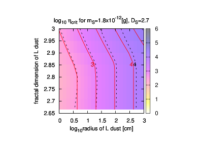
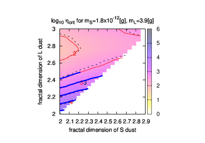
Figure 7: Value of $\eta_{\mathrm{crit}}$ as function of dust radius $r_{{}_{S}}$, $r_{{}_{L}}$ and fractal dimension $D_{{}_{S}}$, $D_{{}_{L}}$. The base values are $r_{{}_{S}}=1.0\times{10}^{-4}\ \mathrm{cm}$, $r_{{}_{L}}=1.0\ \mathrm{cm}$, $m_{{}_{S}}=1.9\times{10}^{-12}\ \mathrm{g}$, $m_{{}_{L}}=3.9\ \mathrm{g}$, $D_{{}_{S}}=2.665$, and $D_{{}_{L}}=3.0$. We keep $m_{\textbf{\tiny{I}}}$ constant when we vary $D_{\textbf{\tiny{I}}}$; we keep $D_{\textbf{\tiny{I}}}$ constant when we vary $r_{\textbf{\tiny{I}}}$. Numerical results are in colour maps and black dashed contours; analytical values in coloured solid contours (c.f. §5.4.4 for the details of the plots.)

The second set of Fig. 7 uses the ‘hard dust’ cross sections, where $r_{{}_{S}}=1.0\times{10}^{-4}\ \mathrm{cm}$, $r_{{}_{L}}=1.0\ \mathrm{cm}$, $m_{{}_{S}}=1.9\times{10}^{-12}\ \mathrm{g}$, $m_{{}_{L}}=3.9\ \mathrm{g}$, $D_{{}_{S}}=2.7$, and $D_{{}_{L}}=3.0$. The critical number density is $\eta_{\mathrm{crit}}=3.01\times{10}^{2}$ for this representative parameter.

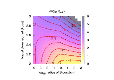
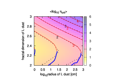
Figure 8: Value of $\eta_{\mathrm{crit}}$ as function of $r_{{}_{S}}$, $r_{{}_{L}}$, $D_{{}_{S}}$, and $D_{{}_{L}}$. Parameters do not appear in x-axis or y-axis are uniformly averaged over the parameter range we accept. Numerical results are in colour maps and black dashed contours; analytical values in coloured solid contours (c.f. §5.4.4 for the details of the plots.)

The third set of Fig. 8, is the $\eta_{\mathrm{crit}}$ averaged over the parameters that do not appear in the axes, to show the tendency of overall dependence on the parameters, and to demonstrate the precision of the analytic formulae.

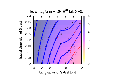
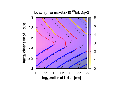
Figure 9: In the above plots, all the parameters but the charge separation efficiency is same as that of Fig. 6, while the the charge separation efficiency $\eta_{ch}=1.0\times{10}^{-5}$ for this figure. Numerical results are in colour maps and black dashed contours; analytical values in coloured solid contours (c.f. §5.4.4 for the details of the plots.)

The fourth set of Fig. 9 uses the same representative dust as in Fig. 6, but is the result of another simulations, where we are now extremely pessimistic and assume that the charge exchange is four orders of magnitude inefficient ($\eta_{ch}=1.0\times{10}^{-5}$ instead of $\eta_{ch}=1.0\times{10}^{-1}$). Even though, the number density $\eta_{\mathrm{crit}}$ required for lightning has raised only by two order of one magnitude. The critical number density is $\eta_{\mathrm{crit}}=6.59\times{10}^{3}$ for the representative parameter.

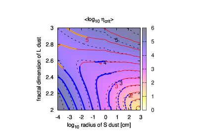
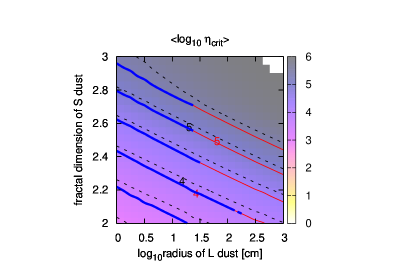
Figure 10: Value of $\eta_{\mathrm{crit}}$ as function of $r_{{}_{S}}$, $r_{{}_{L}}$, $D_{{}_{S}}$, and $D_{{}_{L}}$. Parameters do not appear in x-axis or y-axis are uniformly averaged over the parameter range as in Fig. 8, and we assume $\eta_{ch}=1.0\times{10}^{-5}$ as in Fig. 9. Numerical results are in colour maps and black dashed contours; analytical values in coloured solid contours (c.f. §5.4.4 for the details of the plots.)

The fifth set of Fig. 10 shows the averaged $\eta_{\mathrm{crit}}$ for the pessimistic case $\eta_{ch}=1.0\times{10}^{-5}$. We later examine the accuracy of our formulae by fitting Fig. 10 with the formulae using correction factors determined by Fig. 8 data.

5.4 Analytic formulae for lightning conditions

In this section we derive the analytic form, of $\eta_{\mathrm{crit}}$ and lightning conditions. Numerical results obtained in §5.3 are of great help in deriving these analytic formulae. We show at the end of §5.4.4 that by our analytic formulae we can fit $364325$ numerically-obtained points distributed among six decades with 21 per cent precision. Moreover, the formulae ‘predicts’ results of another simulation with 59 per cent precision, where charge exchange is $10^{4}$ times inefficient. These agreements are good evidences for correctness of both numerical and analytical results.

We made plots like Fig. 3 and Fig. 4 for many points within our parameter space, and found that $\eta=\eta_{\mathrm{crit}}$ is met at the boundary of (c)charge-up phase and (d)dust phase in most cases, and sometimes in (d)dust phase or (c)charge-up phase. Therefore we derive analytic form of $\eta$ corresponding to these three cases in §5.4.1 to §5.4.3, and combine them in §5.4.4

5.4.1 Analytic formulae for charge-up phase / dust phase boundary

We first calculate $\eta^{(cd)}$, the value of $\eta$ corresponding to the (c)charge-up phase / (d)dust phase boundary.

The boundary satisfies $J_{{{}_{L}},{{}_{S}}}=J_{i,{{}_{S}}}$ (Table 4). We use the approximations in (c)charge-up phase to find the break point of the phase. Then

$$J_{{{}_{L}},{{}_{S}}} \simeq 2\pi r_{{}_{S}}r_{{}_{L}}\Delta q_{{{}_{A}},{{}_{C}}}n_{{}_{S}}n_{{}_{L}}\Delta v_{{{}_{L}},{{}_{S}}}$$ (116)

$$J_{{{}_{S}},i} \simeq -Q_{i}n_{{}_{S}}\pi{r_{{}_{S}}}^{2}\sigma_{{{}_{S}},i}v_{i}$$ (117)

because we can ignore the neutralization current $J_{{{}_{L}},{{}_{S}}}^{(n)}$, approximate $\sigma_{{{}_{L}},{{}_{S}}}=\pi{r_{{}_{L}}}^{2}$, $\sigma_{{{}_{S}},i}=\pi{r_{{}_{S}}}^{2}$ (geometric cross sections) and $\sigma_{{{}_{L}},i}=\pi{r_{{}_{L}}}^{2}\left|eQ_{{}_{L}}\right|(r_{{}_{L}}k_{B}Tn_{{}_{L}})^{-1}$ ($qq^{\prime}a^{-1}>\!\!>k_{B}T$ limit of Coulomb cross section (31)).

In dust charge-up phase, both ions and electrons are mainly absorbed by smaller dust, so from (52) and (53) we have

$$Q_{i} = \frac{e\zeta n_{g}}{n_{{}_{S}}\sigma_{{{}_{S}},i}v_{i}}$$ (118)

$$Q_{e} = \frac{-e\zeta n_{g}}{n_{{}_{S}}\sigma_{{{}_{S}},e}v_{e}}$$ (119)

and the absorption cross sections are geometric : $\sigma_{{{}_{S}},i}=\sigma_{{{}_{S}},e}=\pi{r_{{}_{S}}}^{2}$.

By substituting (118) into (117)

$$J_{{{}_{S}},i}=e\zeta n_{g}=J_{e,i}$$ (120)

cf. Fig. 3(c) and in equation (93).

We have come to a simple result, that $\eta_{\mathrm{crit}}$ satisfies

$$J_{{{}_{L}},{{}_{S}}}=J_{e,i}.$$ (121)

Substituting equations (116) , (120), together with $n_{{}_{S}}=\eta^{(cd)}n_{{}_{S}}^{\bowtie}$ and $n_{{}_{L}}=\eta^{(cd)}n_{{}_{L}}^{\bowtie}$ into equation (121) and solving for dust number density $\eta$, we have

$$\eta^{\left(cd\right)}=\left(\frac{\alpha^{\left(cd\right)}}{2\pi}\frac{e}{\Delta q_{{{}_{A}},{{}_{C}}}}\frac{n_{g}}{n_{{}_{S}}^{\bowtie}n_{{}_{L}}^{\bowtie}r_{{}_{S}}r_{{}_{L}}}\frac{\zeta}{\Delta v_{{{}_{L}},{{}_{S}}}}\right)^{\frac{1}{2}}$$ (122)

We have introduced a nondimensional correction factor $\alpha^{(cd)}$, a constant that does not depend on $r_{{}_{S}},r_{{}_{L}},D_{{}_{S}},D_{{}_{L}}$. We need this to compensate the error arising from using the formulae in (c)charge-up phase to find the break point of itself. The actual value for $\alpha^{(cd)}$ is in §5.4.4.

5.4.2 Analytic formula for $\eta_{\mathrm{crit}}$ in dust phase

Next, we derive the analytic formula of the critical density $\eta_{\mathrm{crit}}^{(d)}$, where the condition for electric discharge (63) is met in (d)dust phase (c.f. §5.2.4, Figure 5(d)).

Imposing $J_{{{}_{L}},{{}_{S}}}=0$ in (44), and by approximating the charge neutrality (54) with $Q_{{}_{S}}+Q_{{}_{L}}=0$, we have

$$Q_{{}_{S}}=\left|Q_{{}_{L}}\right|=\Delta q_{{{}_{A}},{{}_{C}}}n_{{}_{S}}\frac{2r_{{}_{S}}}{r_{{}_{L}}}$$ (123)

By approximating equation (53) with $J_{{{}_{S}},e}+J_{i,e}=0$, we have

$$Q_{e} = -\frac{en_{g}\zeta}{\pi n_{{}_{S}}{r_{s}}^{2}\left(1+\chi\right)v_{e}}$$ (124)

$$where\ \ 1+\chi = 1+\frac{Q_{{}_{S}}e}{n_{{}_{S}}r_{{}_{S}}k_{B}T};$$ (125)

the factor $(1+\chi)$ comes from the Coulomb cross section (31).

Substituting $Q_{{}_{L}}$ and $Q_{e}$, the equality for the lightning condition (63) becomes

$$\frac{2\pi\Delta q_{{{}_{A}},{{}_{C}}}}{e}\frac{{n_{s}}^{2}{r_{{}_{S}}}^{3}\left(1+\chi\right)}{n_{g}r_{{}_{L}}}\frac{v_{e}}{\zeta}=\frac{\Delta W_{\mathrm{ion}}}{m_{e}v_{e}u_{{}_{L}}}$$ (126)

By substituting $n_{{}_{S}}=\eta_{\mathrm{crit}}^{(d)}n_{{}_{S}}^{\bowtie}$ and by solving for $\eta_{\mathrm{crit}}^{(d)}$, we have the following analytic formula for $\eta_{\mathrm{crit}}^{(d)}$:

$$\eta_{\mathrm{crit}}^{\left(d\right)}=\left(\frac{\alpha^{\left(d\right)}}{2\pi\left(1+\chi\right)}\frac{e}{\Delta q_{{{}_{A}},{{}_{C}}}}\frac{n_{g}r_{{}_{L}}}{{n_{{}_{S}}^{\bowtie}}^{2}{r_{{}_{S}}}^{3}}\frac{\zeta}{u_{{}_{L}}}\frac{\Delta W_{\mathrm{ion}}}{k_{B}T}\right)^{\frac{1}{2}}.$$ (127)

We have introduced another nondimensional correction constant $\alpha^{(d)}$ as we did in §5.4.1.

5.4.3 Analytic formula for $\eta_{\mathrm{crit}}$ in charge-up phase

Finally, we derive the analytic formula of the critical density $\eta_{\mathrm{crit}}^{(c)}$, where the condition for electric discharge (63) is met in (c)charge-up phase (c.f. §5.2.3, Figure 5(c)).

By approximating equations (52) and (54) with $J_{{{}_{S}},i}=J_{i,e}$ and $Q_{{}_{S}}+Q_{i}=0$, we have

$$Q_{i}=-Q_{{}_{S}}=\frac{en_{g}\zeta}{\pi n_{{}_{S}}{r_{{}_{S}}}^{2}v_{i}}$$ (128)

In equation (50), we can ignore $J_{{{}_{L}},e}$ and further ignoring the second term in equation (44), we have

$$\frac{2r_{{}_{S}}}{r_{{}_{L}}}\Delta q_{{{}_{A}},{{}_{C}}}n_{{}_{S}}n_{{}_{L}}\Delta v_{{{}_{L}},{{}_{S}}}\pi{r_{{}_{L}}}^{2}-Q_{i}n_{{}_{L}}\sigma_{{{}_{L}},i}v_{i}=0$$ (129)

$$where\ \ \sigma_{{{}_{L}},i}=\frac{Q_{{}_{L}}e}{n_{{}_{L}}r_{{}_{L}}l_{B}T}\pi{r_{{}_{L}}}^{2}$$ (130)

here we used the $qq^{\prime}a^{-1}>\!\!>k_{B}T$ limit of Coulomb cross section (31).

Solving this for $Q_{{}_{L}}$, we have

$$\left|Q_{{}_{L}}\right|=\frac{2\Delta q_{{{}_{A}},{{}_{C}}}}{e^{2}}\frac{{n_{{}_{S}}}^{2}n_{{}_{L}}{r_{{}_{S}}}^{3}}{n_{g}}\frac{\Delta v_{{{}_{L}},{{}_{S}}}k_{B}T}{\zeta}$$ (131)

And from equation (53) we have

$$Q_{e}=-\frac{en_{g}\zeta}{\pi n_{{}_{S}}{r_{{}_{S}}}^{2}v_{e}}$$ (132)

By substituting these $Q_{{}_{L}}$ and $Q_{e}$ to the equality for the lightning condition (63), replacing $n_{{}_{S}}=\eta_{\mathrm{crit}}^{(c)}n_{{}_{S}}^{\bowtie}$ and $n_{{}_{L}}=\eta_{\mathrm{crit}}^{(c)}n_{{}_{L}}^{\bowtie}$, and by solving for $\eta_{\mathrm{crit}}^{(c)}$, we obtain the following analytic formula for $\eta_{\mathrm{crit}}^{(c)}$:

$$\eta_{\mathrm{crit}}^{\left(c\right)}=\left(\frac{\alpha^{\left(c\right)}}{2\pi}\frac{e^{3}}{\Delta q_{{{}_{A}},{{}_{C}}}}\frac{{n_{g}}^{2}}{{n_{{}_{S}}^{\bowtie}}^{3}{n_{{}_{L}}^{\bowtie}}{r_{{}_{S}}}^{5}}\frac{\zeta^{2}}{\Delta v_{{{}_{L}},{{}_{S}}}u_{{}_{L}}}\frac{\Delta W_{\mathrm{ion}}}{\left(k_{B}T\right)^{2}}\right)^{\frac{1}{4}}$$ (133)

We have introduced a third nondimensional correction constant $\alpha^{(c)}$ as we did in previous sections.

5.4.4 The combined analytic formula for $\eta_{\mathrm{crit}}$

The critical number density $\eta_{\mathrm{crit}}$ is either of $\eta_{\mathrm{crit}}^{(c)},\eta^{(cd)},\eta_{\mathrm{crit}}^{(d)}$. To choose the correct one, we have to consider the phase boundary conditions (c.f. Table 4). Instead, we propose the following convenient scheme to choose the correct one:

$$\eta_{\mathrm{crit}} = \eta_{\mathrm{crit}}^{\left(d\right)}\ \ \ \ if\ \ \eta_{\mathrm{crit}}^{\left(d\right)}>\eta^{\left(cd\right)},$$ (134)

$$= \eta^{\left(cd\right)}\ \ \ \ if\ \ \eta_{\mathrm{crit}}^{\left(c\right)}>\eta^{\left(cd\right)}>\eta_{\mathrm{crit}}^{\left(d\right)},$$

$$= \eta_{\mathrm{crit}}^{\left(c\right)}\ \ \ \ otherwise.$$

This scheme is based on the intuition that the (cd)phase boundary is included in both (c)charge-up phase and (d)dust phase. We can argue that if $\eta_{\mathrm{crit}}^{(d)}>\eta^{(cd)}$, the number density $\eta^{(cd)}$ is not large enough to cause lightning, and that if $\eta_{\mathrm{crit}}^{(c)}<\eta^{(cd)}$, the number density $\eta_{\mathrm{crit}}^{(c)}$ is already large enough to cause lightning.

Now, without the correction, e.g. with $\alpha^{(c)}=\alpha^{(cd)}=\alpha^{(d)}=1$, the analytic values for $\eta_{\mathrm{crit}}$ differs from the numerical values $\eta_{\mathrm{crit}}^{(num)}$ calculated in §5.3, because of approximations used. For example, substituting the reference parameter of Fig. 6: $r_{{}_{S}}=1.0\times{10}^{-2}\ \mathrm{cm}$, $r_{{}_{L}}=1.0\times{10}^{2}\ \mathrm{cm}$, $D_{{}_{S}}=2.0$, and $D_{{}_{L}}=2.368$, equation (134) evaluates to $\eta_{\mathrm{crit}}=1.47\times{10}^{2}$. For the reference parameter of Fig. 7: $r_{{}_{S}}=1.0\times{10}^{-4}\ \mathrm{cm}$, $r_{{}_{L}}=1.0\ \mathrm{cm}$, $D_{{}_{S}}=2.665$, and $D_{{}_{L}}=3.0$, equation (134) evaluates to $\eta_{\mathrm{crit}}=9.99\times{10}^{2}$. The results of the simulations for those two parameter are $\eta_{\mathrm{crit}}^{(num)}=7.37\times{10}^{1}$ and $\eta_{\mathrm{crit}}^{(num)}=3.01\times{10}^{2}$, respectively. The analytic and simulational values agree upto a factor of three.

We set the values for $\alpha^{(c)},\alpha^{(cd)},\alpha^{(d)}$ by the condition that the following squared-error integral over the entire parameter ranges (109-115) is minimum:

$$\int\!\!\!\int\!\!\!\int\!\!\!\int dr_{{}_{S}}\,dr_{{}_{L}}\,dD_{{}_{S}}\,dD_{{}_{L}}\left(\log_{10}\eta_{\mathrm{crit}}-\log_{10}\eta_{\mathrm{crit}}^{\left(num\right)}\right)^{2}$$ (135)

This gives $\alpha^{(c)}=9.4\times{10}^{-1},\alpha^{(cd)}=3.3\times{10}^{-1},\alpha^{(d)}=8.5\times{10}^{-1}$. Taking these corrections into account, the values for $\eta^{(c)},\eta^{(cd)},\eta^{(d)}$ are as follows:

$$\eta^{\left(c\right)}_{\mathrm{crit}} = 1.1\times{10}^{3}\left(\frac{\Delta q_{{{}_{A}},{{}_{C}}}}{6.2\times{10}^{2}\ \mathrm{e}}\right)^{-\frac{1}{4}}\left(\frac{n_{g}}{4.7\times{10}^{13}\ \mathrm{cm^{-3}}}\right)^{\frac{1}{2}}$$ (136)

$$\left(\frac{n_{{}_{S}}^{\bowtie}}{8.8\times{10}^{-1}\ \mathrm{cm^{-3}}}\right)^{-\frac{3}{4}}\left(\frac{n_{{}_{L}}^{\bowtie}}{4.0\times{10}^{-14}\ \mathrm{cm^{-3}}}\right)^{-\frac{1}{4}}$$

$$\left(\frac{r_{{}_{S}}}{1.0\times{10}^{-4}\ \mathrm{cm}}\right)^{-\frac{5}{4}}$$

$$\left(\frac{\zeta}{1.0\times{10}^{-18}\ \mathrm{sec^{-1}}}\right)^{\frac{1}{2}}$$

$$\left(\frac{\Delta v_{{{}_{L}},{{}_{S}}}}{3.4\times{10}^{3}\ \mathrm{cm\ sec^{-1}}}\right)^{-\frac{1}{4}}\left(\frac{u_{{}_{L}}}{3.4\times{10}^{3}\ \mathrm{cm\ sec^{-1}}}\right)^{-\frac{1}{4}}$$

$$\left(\frac{\Delta W_{\mathrm{ion}}}{15.4\ \mathrm{eV}}\right)^{\frac{1}{2}}\left(\frac{T}{1.7\times{10}^{2}\ \mathrm{K}}\right)^{-\frac{1}{2}},$$

$$\eta^{\left(cd\right)} = 3.3\times{10}^{2}\left(\frac{\Delta q_{{{}_{A}},{{}_{C}}}}{6.2\times{10}^{2}\ \mathrm{e}}\right)^{-\frac{1}{2}}\left(\frac{n_{g}}{4.7\times{10}^{13}\ \mathrm{cm^{-3}}}\right)^{\frac{1}{2}}$$ (137)

$$\left(\frac{n_{{}_{S}}^{\bowtie}}{8.8\times{10}^{-1}\ \mathrm{cm^{-3}}}\right)^{-\frac{1}{2}}\left(\frac{n_{{}_{L}}^{\bowtie}}{4.0\times{10}^{-14}\ \mathrm{cm^{-3}}}\right)^{-\frac{1}{2}}$$

$$\left(\frac{r_{{}_{S}}}{1.0\times{10}^{-4}\ \mathrm{cm}}\right)^{-\frac{1}{2}}\left(\frac{r_{{}_{L}}}{1.0\ \mathrm{cm}}\right)^{-\frac{1}{2}}$$

$$\left(\frac{\zeta}{1.0\times{10}^{-18}\ \mathrm{sec^{-1}}}\right)^{\frac{1}{2}}$$

$$\left(\frac{\Delta v_{{{}_{L}},{{}_{S}}}}{3.4\times{10}^{3}\ \mathrm{cm\ sec^{-1}}}\right)^{-\frac{1}{2}},$$

$$\eta^{\left(d\right)}_{\mathrm{crit}} = 5.9\times{10}^{1}\left(\frac{\Delta q_{{{}_{A}},{{}_{C}}}}{6.2\times{10}^{2}\ \mathrm{e}}\right)^{-\frac{1}{2}}\left(\frac{n_{g}}{4.7\times{10}^{13}\ \mathrm{cm^{-3}}}\right)^{\frac{1}{2}}$$ (138)

$$\left(\frac{n_{{}_{S}}^{\bowtie}}{8.8\times{10}^{-1}\ \mathrm{cm^{-3}}}\right)^{-1}$$

$$\left(\frac{r_{{}_{S}}}{1.0\times{10}^{-4}\ \mathrm{cm}}\right)^{-\frac{3}{2}}\left(\frac{r_{{}_{L}}}{1.0\ \mathrm{cm}}\right)^{\frac{1}{2}}$$

$$\left(\frac{\zeta}{1.0\times{10}^{-18}\ \mathrm{sec^{-1}}}\right)^{\frac{1}{2}}\left(\frac{u_{{}_{L}}}{3.4\times{10}^{3}\ \mathrm{cm\ sec^{-1}}}\right)^{-\frac{1}{2}}$$

$$\left(\frac{\Delta W_{\mathrm{ion}}}{15.4\ \mathrm{eV}}\right)^{\frac{1}{2}}\left(\frac{T}{1.7\times{10}^{2}\ \mathrm{K}}\right)^{-\frac{1}{2}}.$$

Note that $\Delta q_{{{}_{A}},{{}_{C}}}$, $n_{{}_{S}}^{\bowtie}$, and $n_{{}_{L}}^{\bowtie}$ also depends on dust parameters: $r_{{}_{S}}$, $r_{{}_{L}}$, $D_{{}_{S}}$, and $D_{{}_{L}}$. Using equation (38) and the $\eta_{ch},\sigma_{ch}$ introduced in §3.4.1,

$$\Delta q_{{{}_{A}},{{}_{C}}} = \eta_{ch}\sigma_{ch}S_{\mathrm{kiss}}$$ (140)

$$= 6.2\times{10}^{2}\ \mathrm{e}\cdot\frac{\eta_{ch}}{0.1}\frac{\sigma_{ch}}{6.2\times{10}^{9}\ \mathrm{e\ cm^{-2}}}$$

$$\frac{{\mathrm{min}}\left({r_{{}_{S}}}^{3/2}{r_{{}_{L}}}^{1/2},{r_{m}}^{2-D_{{}_{L}}}{r_{{}_{S}}}^{5/2}{r_{{}_{L}}}^{D_{{}_{L}}-5/2}\right)}{1.0\times{10}^{-6}\ \mathrm{cm^{2}}}.$$

Using equations (5-11) and equation (29),

$$n_{{}_{S}}^{\bowtie} = 4.0\times{10}^{2}\left(\frac{r_{{}_{S}}}{r_{m}}\right)^{-D_{{}_{S}}}\ \mathrm{cm^{-3}}$$ (141)

$$\left(\frac{r}{2.7\ \mathrm{AU}}\right)^{-11/4}\left(\frac{m_{m}}{3.9\times{10}^{-15}\ \mathrm{g}}\right)^{-1}$$

$$n_{{}_{L}}^{\bowtie} = 4.0\times{10}^{1}\left(\frac{r_{{}_{L}}}{r_{m}}\right)^{-D_{{}_{L}}}\ \mathrm{cm^{-3}}$$ (142)

$$\left(\frac{r}{2.7\ \mathrm{AU}}\right)^{-11/4}\left(\frac{m_{m}}{3.9\times{10}^{-15}\ \mathrm{g}}\right)^{-1},$$

and the monomer radius

$$r_{m}=1.0\times{10}^{-5}\ \mathrm{cm}.$$ (143)

We have plotted these analytic solutions (136-138) combined with the condition (134) in solid-line contours from Fig. 6 to Fig. 8. The red thin contour represents the parameter ranges where $\eta^{(cd)}$ contributes. The blue thick contours represents the parameter ranges where $\eta^{(d)}$ contributes, where blue solid contour means $\chi<1$ and blue dashed contour $\chi>1$. The thick yellow-sleeved red contours represents the parameter ranges where $\eta^{(c)}$ contributes. The numerical solutions, on the other hand, are plotted in colour maps and the black dashed contours.

The averaged plots, Fig. 8 shows the agreement of the numerical and analytic value over the entire parameter range. Quantitatively, the root-mean-square error is

$$\sqrt{\frac{\int\!\!\!\int\!\!\!\int\!\!\!\int dr_{{}_{S}}\,dr_{{}_{L}}\,dD_{{}_{S}}\,dD_{{}_{L}}\left(\log_{10}\eta_{\mathrm{crit}}-\log_{10}\eta_{\mathrm{crit}}^{\left(num\right)}\right)^{2}}{\int\!\!\!\int\!\!\!\int\!\!\!\int dr_{{}_{S}}\,dr_{{}_{L}}\,dD_{{}_{S}}\,dD_{{}_{L}}}}$$

$$=9.2\times{10}^{-2}.$$ (144)

Moreover, using the values of $\alpha^{(c)},\alpha^{(cd)},\alpha^{(d)}$ obtained only from the ‘normal’ run (Fig. 6, 7 and 8), we can fit the results of the ‘pessimistic’ simulations (Fig. 9) by a root-mean-square error of $2.6\times{10}^{-1}$. We also perform the simulations with smaller values of relative velocity and fit the results. The root-mean-square errors were $5.6\times{10}^{-2},6.4\times{10}^{-2},1.1\times{10}^{-1}$, for $\Delta v_{{{}_{L}},{{}_{S}}}=u_{{}_{L}}=3.4\times{10}^{2}\ \mathrm{cm\ s^{-1}},3.4\times{10}^{1}\ \mathrm{cm\ s^{-1}},3.4\ \mathrm{cm\ s^{-1}}$, respectively. These fits prove the predictability of our analytic formulae (134) and (136-138).

6 Conclusions and discussions

We have shown that as dust number density $\eta$ increase, the charge density distribution experience four phases: (a)ion-electron plasma phase, (b)ion-dust plasma phase, (c)charge-up phase and (d)dust phase. The former two phases are studied in detail by Okuzumi (2009), while the latter two phases are unique results of taking dust-dust collision into consideration. We have calculated the dust number density $\eta_{\mathrm{crit}}$ at which lightning strikes, as function of dust radius $r_{{}_{S}}$, $r_{{}_{L}}$ and fractal dimension $D_{{}_{S}}$, $D_{{}_{L}}$ numerically. Using the numerical results we have derived the analytical formulae for $\eta_{\mathrm{crit}}$: equations (134), (136-138). Because the generated electrostatic field $E_{\mathrm{max}}(\eta)$ grows more rapidly than estimate by Gibbard et al. (1997) in (c)charge-up phase and (d)dust phase, lightning in protoplanetary discs are possible with smaller dust number densities. We discuss the consequences in this section.

6.1 Energetics and direct observations

We estimate the total energy of a lightning event in a protoplanetary disc at $r=2.7\ \mathrm{AU}$. For MMSN, the number density of the gas is $4.7\times{10}^{13}\ \mathrm{cm^{-3}}$ in the region. The typical electron mean free path at this site is $l_{mfp}\simeq 1.2\times{10}^{2}\ \mathrm{cm}$. By equation (56) we know the critical electric field $E_{\mathrm{dis}}\simeq 4.3\times{10}^{-4}\ \mathrm{G}$. The sphere with radius of the disc scale-height $h\simeq 2.4\times{10}^{12}\ \mathrm{cm}$ contains the electric energy $W\equiv{E_{\mathrm{dis}}}^{2}/8\pi\times 4\pi h^{3}/3\simeq 4.3\times{10}^{29}\ \mathrm{erg}$. When the lightning strikes, the energy is concentrated into lightning bolt of radius $w$ and length $h$, where $w$ is related to $l_{mfp}$ by $w\simeq 5000\,l_{mfp}\simeq 6.0\times{10}^{5}\ \mathrm{cm}$ (Pilipp et al., 1992). If all the energy is used to heat the gas within the lightning bolt, the gas can be heated to $1.6\times{10}^{7}\ \mathrm{K}$.

The ultimate energy source for this electric discharge event is the gravitational energy of the accreting matter. In our model the mass accretion ratio of uncondensed larger dust is $\dot{M}=2\pi r\Sigma_{{}_{L}}^{\bowtie}u_{{}_{L}}\simeq 3.3\times{10}^{17}\ \mathrm{g\ sec^{-1}}$. The gravitational energy released within condensation region $h$ is $L\equiv GM_{\odot}\dot{M}hr^{-2}\simeq 6.6\times{10}^{28}\ \mathrm{erg\ sec^{-1}}$. For the largest energy event $W=4.3\times{10}^{29}\ \mathrm{erg}$, The upper limit of the event rate is $1.5\times{10}^{-1}\ \mathrm{sec^{-1}}$.

6.1.1 Astronomically Low Frequency (ALF) Waves

The change density evolution, electromagnetic pulse, and electromagnetic waves accompanying lightning in terrestrial thunderclouds are observed (e.g. Koshak & Krider, 1989; Lin et al., 1979). The typical wavelength of the electromagnetic waves are similar to the scale height of the thundercloud. These are called extremely low frequency waves. The electromagnetic waves from lightning can be basically modelled as solutions of Maxwell equations, including lightning current as a source term (e.g. Rakov & Uman, 1998). When we apply these models to the protoplanetary discs, the electromagnetic wave spectrum is extend between the event duration and light crossing time of the system, or $9.6\times{10}^{-5}\sim 1.2\times{10}^{-2}\ \mathrm{Hz}$. This frequency range is at least two orders of magnitude lower than any frequencies with established observational methods. It is difficult to make a fair choice for the successor to the frequency list ‘very low frequency (VLF),’ ‘ultra low frequency(ULF),’ ‘super low frequency (SLF),’ and ‘extremely low frequency (ELF).’ We opt for Astronomically Low Frequency (ALF) waves and hope that the reader will forgive us! Anyway the frequency is so low that we will need an astronomical budget to build an astronomically large detector to receive it, considering its wavelength of order of an astronomical unit.

6.1.2 Infrared (IR) Observations

The energy of the lightning contributes to the local heating of the protoplanetary discs, which might be resolved by advanced telescopes such as Atacama Large Millimetre Array (ALMA). The most possible observational evidence is excess of heating near the snowline. To distinguish the cause of the heating with other heating model candidates, the variability or correlation function of the heating might be useful. This is because lightning propagates at the speed of ionised electrons, which is much faster than the speed of sound.

6.1.3 Ultraviolet (UV) Observations

The ionisation electrons of the lightning excite various electron levels in gas molecules and dust. There is possibility of observing fluorescence photons from such excited molecules. Although the disc gas is generally expected to be thick for ultraviolet photons, there are categories of lightning that extends toward thin regions of the gas, known as sprites and elves (e.g. Williams, 2001). The sprites and elves are phenomena similar to lightning observed in the mesosphere of the earth, possibly caused by electric fields induced by the thunderclouds. Fluorescence lines from such regions can be observed by future ultraviolet missions like THEIA (Spergel et al., 2009). Also, some observational results on protostellar and protoplanetary systems today have difficulties in explaining either lack or excess of UV (e.g. Nomura & Millar, 2005; Chapillon et al., 2008; Pérez et al., 2008; Herczeg & Hillenbrand, 2008). If excess of UV photons is observed compared to the model, it might be from the sprite discharges and elves from the surface of the protoplanetary discs; on the other hand if the chemical composition model require more UV photons than is observed, lightning hidden in the disc mid-plane might be providing them.

6.1.4 High Energy Gamma Rays

Detection of burst-like gamma-ray is reported from terrestrial thunder clouds. The burst precedes a cloud-to-ground lightning, lasts for $\sim 40$ seconds, extends to $10\ \mathrm{MeV}$. The spectrum can be interpreted as consisting of bremsstrahlung photons from relativistic electrons (Tsuchiya et al., 2007; Enoto et al., 2008). These relativistic electrons are secondary electrons generated by cosmic rays, and accelerated by the electric fields through process known as avalanche amplification (Roussel-Dupré & Gurevich, 1996). If a charged particle is accelerated by the protoplanetary thundercloud field, through similar process, its kinetic energy reaches $eEh\simeq 3.1\times{10}^{11}\ \mathrm{eV}$.

6.2 Chondrule heating by lightning

Chondrule heating by lightning scenario is now considered unlikely (Weidnschilling, 1997; Gibbard et al., 1997; Güttler et al., 2008). The reasons that prohibit the scenario can be summarized as following three problems.

6.2.1 Energetics problem

The ultimate energy source (gravitational potential of the protoplanetary disc) is sufficient to melt the chondrules; but most of the energy earned by ingoing larger dust go to the outgoing gas by angular momentum exchange (Weidnschilling, 1997); little contribute to the random motion, the energy source for the lightning.

6.2.2 Neutralization problem

Unlike the earth atmosphere, the protoplanetary discs are filled with weakly ionised plasma which rapidly responds to electric field. Neutralization effect can be further subdivided to microscopic neutralization of individual dust and macroscopic neutralization of large-scale electric field necessary to cause lightning. If a dust get charged by dust-dust collision, the dust absorbs plasma of opposite polarity in $\sim 10\ \mathrm{sec}$ and returns to equilibrium charge state. Moreover, even if there is charged dust and bulk motion between the oppositely charged dust, the electric field caused by the dust induces Ohmic current in the plasma. The current will quickly neutralize the electric field.

6.2.3 Destruction problem

After all, there is an experimental evidence by Güttler et al. (2008) that lightning destroys the dust aggregates rather than melting them.

6.2.4 Solution to the problems

This work can provide answer for the first and second problem. energetics problem, the larger dust and the gas (containing smaller dust that are coupled to the gas) is now ‘harnessed’ by electric field. Outgoing gas is not free in carrying the gravitational energy away; instead the gas converts its gravitational energy into electric field energy, fully contributing to lightning. For the neutralization problem, we have shown in this work that with reasonably high dust number density $\eta$, the dust-dust charge separation can dominate over the plasma neutralization, and the electrostatic field can grow up to critical value.

For the third problem, we point out that in Güttler et al. (2008)’s experiment, either the electron mean free path is many orders of magnitude shorter, or the electron kinetic energy is much larger compared to the protoplanetary-disc environment. They used air at pressures between $10$ and $10^{5}\ \mathrm{Pa}$. Air consists of $78$ per cent nitrogen, $21$ per cent oxygen, and $1$ per cent argon. Their molecular van der Waals radii are $1.6\times{10}^{-8}\ \mathrm{cm}$, $1.5\times{10}^{-8}\ \mathrm{cm}$, and $1.9\times{10}^{-8}\ \mathrm{cm}$, respectively (Bondi, 1964).

Therefore, the electron mean free path and the electron kinetic energy, $W_{e}=e\,E\,l_{\mathrm{mfp}}$, was $l_{\mathrm{mfp}}\sim 4.8\times{10}^{-1}\ \mathrm{cm}$, $W_{e}=1.6\times{10}^{4}\ \mathrm{eV}$ for $10\ \mathrm{Pa}$ case, and $l_{\mathrm{mfp}}\sim 4.8\times{10}^{-5}\ \mathrm{cm}$ , $W_{e}=1.6\ \mathrm{eV}$ for $10^{5}\ \mathrm{Pa}$ case, respectively. On the other hand in protoplanetary discs, typical mean free path and electron kinetic energy are $l_{\mathrm{mfp}}=1.2\times{10}^{2}\ \mathrm{cm}$, $W_{e}=15.4\ \mathrm{eV}$.

It might be possible that protoplanetary-disc lightning is effective in melting dust aggregates, although experimental lightning is ineffective in heating and led to disruption of the dust, due to shorter mean free path or higher energy electron. The minimum size of the structures that electron can form is of order of its mean free path. If the electron mean free path is much shorter than the dust aggregates, as in $10^{5}\ \mathrm{Pa}$ case, the electron current may concentrate on the most conductive part of the dust aggregate, leading to partial heating and explosion of the dust. On the other hand if the electron is much more energetic, as in $10\ \mathrm{Pa}$ case, it may react differently on dust monomers.

To reproduce the mean free path and electron energy simultaneously, one must reproduce the electric field strength $E=4.3\times{10}^{-4}\ \mathrm{G}$ of protoplanetary discs; while the electric field used in the experiment $E=1.1\times{10}^{2}\ \mathrm{G}$ was much stronger. This much stronger electric field itself, might be the cause of dust aggregate dissociation, due to much stronger electric force exerted on electron-absorbed dust monomers. Also the discharge time-scale in the experiment was much smaller than that in the protoplanetary discs, which might have led to the catastrophic results.

We think that the effect of lighting on dust aggregate in protoplanetary-disc environment is yet to be confirmed in future experiments and simulations.

6.3 Effects on magnetorotational instability (MRI) and disc environment

The dust-dust collisional charging and lightning is not a side-effect of some other processes, but is one of the key processes in protoplanetary discs that affects each other. The lightning is powered by gravitational energy of the migrating larger dust. The migration of the larger dust as well as the long term evolution of the gas disc is governed by the disc viscosity. The best candidate for providing the disc viscosity is MRI. And MRI is controlled by gas ionisation degree, which in turn is controlled by the dust charge state and lightning.

Even the longest estimate for time-scale of the lightning $1.0\times{10}^{4}\ \mathrm{sec}$ is much smaller than the time-scale of MRI, which is at least of the order of Kepler timescales. Lightning occur in low-ionisation regions where MRI is prohibited (dead zones), and even if the lightning instantly raise the ionisation rate, the free electrons and ions will quickly be absorbed by the dust. Therefore we expect that MRI and lightning cannot co-exist. However lot of profound phenomena are possible. Just for an example let us think of a two-layer dead-active zone model but with dust-dust collisional charging. The dead-zone is filled with lightning, inducing sprite discharges towards active zones, which sustains the ionisation rate and MRI. The MRI in turn shovels the dust into the dead-zone.

Such global models are beyond the reach of this paper. Nevertheless we conclude this paper by stating that the dust-dust collisional charging is a necessary component for understanding the planetesimal formation and global behaviour of the protoplanetary discs.

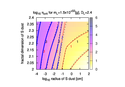
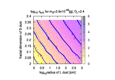
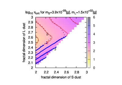
Figure 6: Value of $\eta_{\mathrm{crit}}$ as function of dust radius $r_{{}_{S}}$, $r_{{}_{L}}$ and fractal dimension $D_{{}_{S}}$, $D_{{}_{L}}$. The base values are $r_{{}_{S}}=1.0\times{10}^{-2}\ \mathrm{cm}$, $r_{{}_{L}}=1.0\times{10}^{2}\ \mathrm{cm}$, $m_{{}_{S}}=3.9\times{10}^{-9}\ \mathrm{g}$, $m_{{}_{L}}=1.5\times{10}^{2}\ \mathrm{g}$, $D_{{}_{S}}=2.0$, and $D_{{}_{L}}=2.368$. We keep $m_{\textbf{\tiny{I}}}$ constant when we vary $D_{\textbf{\tiny{I}}}$; we keep $D_{\textbf{\tiny{I}}}$ constant when we vary $r_{\textbf{\tiny{I}}}$. Numerical results are in colour maps and black dashed contours; analytical values in coloured solid contours (c.f. §5.4.4 for the details of the plots.)

Appendix A Cationic dust and anionic dust

In this section we justify the two-dust picture introduced in §2.1. Protoplanetary discs consist of dust with various parameter J. The parameter vector J may include, but is not limited to, dust radius, porosity, material and surface chemical potential. We classify these dust into two groups according to their electric tendency; one is cationic dust who receive positive charge through dust-dust collision and the other is anionic dust who receive negative charge. In this section we give the precise definition of cationic and anionic dust.

Let $n_{\textbf{\tiny\em{J}}}$ indicate the number density of the dust with parameter J. Let $\sigma_{{\textbf{\tiny\em{J}}}^{\prime},{\textbf{\tiny\em{J}}}}$, $\Delta v_{{\textbf{\tiny\em{J}}}^{\prime},{\textbf{\tiny\em{J}}}}$, $\Delta q_{{\textbf{\tiny\em{J}}}^{\prime},{\textbf{\tiny\em{J}}}}$ be collisional cross section, mean relative velocity, and mean amount of charge that moves from dust ${\textbf{\em J}}^{\prime}$ to dust J in a collision, respectively. Then we can calculate $\dot{q}_{\textbf{\tiny\em{J}}}$, charge received by dust J per unit time, by

$$\dot{q}_{\textbf{\tiny\em{J}}}=\sum_{{\textbf{\em J}}^{\prime}}\Delta q_{{\textbf{\tiny\em{J}}}^{\prime},{\textbf{\tiny\em{J}}}}n_{{\textbf{\tiny\em{J}}}^{\prime}}\sigma_{{\textbf{\tiny\em{J}}}^{\prime},{\textbf{\tiny\em{J}}}}\Delta v_{{\textbf{\tiny\em{J}}}^{\prime},{\textbf{\tiny\em{J}}}}.$$ (145)

We define cationic dust and anionic dust as $C\equiv\{{\textbf{\em J}}|\dot{q}_{\textbf{\tiny\em{J}}}>0\}$ and $A\equiv\{{\textbf{\em J}}|\dot{q}_{\textbf{\tiny\em{J}}}<0\}$. Cationic dust receive net positive charge in dust-dust collision and tend to be cationic, while anionic dust tend to be anionic.

We assume the average dust distribution $n^{(0)}_{\textbf{\tiny\em{J}}}$ as that of MMSN model. We also assume that at some local condensation regions, dust number density is multiplied by carrying in dust from other portions of the disk. For simplicity we assume that the relative number density $\eta$ is independent of dust parameter J so that $n_{\textbf{\tiny\em{J}}}=\eta n^{(0)}_{\textbf{\tiny\em{J}}}$ (e.g. this is the case when collisional cascade equilibrium is faster than the migration). We define $\sigma_{{\textbf{\tiny\em{J}}}^{\prime},{\textbf{\tiny\em{J}}}}$ and $\Delta q_{{\textbf{\tiny\em{J}}}^{\prime},{\textbf{\tiny\em{J}}}}$ as the value for neutral dust. As the dust acquires charge, the amount of charge exchanged in a single collision becomes smaller due to the exchange of the charge they already have; we treat this deviation from neutral dust as separate ‘neutralization’ channel. With these assumptions, the sign of $\dot{q}_{\textbf{\tiny\em{J}}}$ (145) do not depend on $\eta$, and the term ‘cationic dust’ and ‘anionic dust’ is well defined independent of dust number density $\eta$.

Now we can simplify the problem by treat cationic and anionic dust as if they are two discrete kinds of dust. Therefore we define the representative variables for cationic and anionic dust as follows.

$$n_{{}_{C}} = \sum_{{\textbf{\tiny\em{J}}}\in C}\ n_{{\textbf{\tiny\em{J}}}}=\eta\sum_{{\textbf{\tiny\em{J}}}\in C}\ n^{\left(0\right)}_{{\textbf{\tiny\em{J}}}}$$ (146)

$$n_{{}_{A}} = \sum_{{\textbf{\tiny\em{J}}}\in A}\ n_{{\textbf{\tiny\em{J}}}}=\eta\sum_{{\textbf{\tiny\em{J}}}\in A}\ n^{\left(0\right)}_{{\textbf{\tiny\em{J}}}}$$ (147)

$$v_{{{}_{A}},{{}_{C}}} = \frac{\sum_{{\textbf{\tiny\em{J}}}\in A,{\textbf{\tiny\em{J}}}^{\prime}\in C}\ n_{{\textbf{\tiny\em{J}}}}n_{{\textbf{\tiny\em{J}}}^{\prime}}v_{{\textbf{\tiny\em{J}}},{\textbf{\tiny\em{J}}}^{\prime}}}{n_{{}_{C}}n_{{}_{A}}}$$ (148)

$$\sigma_{{{}_{A}},{{}_{C}}} = \frac{\sum_{{\textbf{\tiny\em{J}}}\in A,{\textbf{\tiny\em{J}}}^{\prime}\in C}\ \sigma_{{\textbf{\tiny\em{J}}},{\textbf{\tiny\em{J}}}^{\prime}}\,n_{{\textbf{\tiny\em{J}}}}\,n_{{\textbf{\tiny\em{J}}}^{\prime}}\,v_{{\textbf{\tiny\em{J}}},{\textbf{\tiny\em{J}}}^{\prime}}}{\sum_{{\textbf{\tiny\em{J}}}\in A,{\textbf{\tiny\em{J}}}^{\prime}\in C}\ n_{{\textbf{\tiny\em{J}}}}n_{{\textbf{\tiny\em{J}}}^{\prime}}v_{{\textbf{\tiny\em{J}}},{\textbf{\tiny\em{J}}}^{\prime}}}$$ (149)

$$\Delta q_{{{}_{A}},{{}_{C}}} = \frac{\sum_{{\textbf{\tiny\em{J}}}\in A,{\textbf{\tiny\em{J}}}^{\prime}\in C}\ \Delta q_{{\textbf{\tiny\em{J}}},{\textbf{\tiny\em{J}}}^{\prime}}\sigma_{{\textbf{\tiny\em{J}}},{\textbf{\tiny\em{J}}}^{\prime}}\,n_{{\textbf{\tiny\em{J}}}}\,n_{{\textbf{\tiny\em{J}}}^{\prime}}\,v_{{\textbf{\tiny\em{J}}},{\textbf{\tiny\em{J}}}^{\prime}}}{\sum_{{\textbf{\tiny\em{J}}}\in C,{\textbf{\tiny\em{J}}}^{\prime}\in A}\ \sigma_{{\textbf{\tiny\em{J}}},{\textbf{\tiny\em{J}}}^{\prime}}\,n_{{\textbf{\tiny\em{J}}}}\,n_{{\textbf{\tiny\em{J}}}^{\prime}}\,v_{{\textbf{\tiny\em{J}}},{\textbf{\tiny\em{J}}}^{\prime}}}.$$ (150)

Appendix B Simulations

In this section, we briefly describe our numerical methods. We need to solve the equilibrium equations (50-54), for various environmental parameters. Especially we vary $\eta$ for each set of other parameters. Then we know the minimum $\eta$ that satisfies the electric discharge condition (63), for the each set of other parameters.

This kind of problem, a massive parameter parallelism, is typically suitable for massively parallel computing hardware (e.g. Ford, 2009), such as general purpose graphic processors (GPGPUs) or GRAPE-DR (Makino, 2008). We describe the CPU and GPGPU based programmes we used in this research to solve equations (40-43) in this section.

B.1 Direct integral solver

The most straightforward means of finding the equilibrium solutions (40-43) is to directly integrate the dynamic equations (40-43). Nevertheless, constant-time-step direct integral cannot solve (40-43) correctly for some of the parameter range. This is because the current densities $Q_{\textbf{\tiny{I}}}$ differ many orders of magnitude for such parameters. We must choose the integration time-step $dt_{i}$ carefully. This leads us to the use of a adaptive time step.

The adaptive-time-step direct-integral solver follows the dynamic equations (40-43) in terms of discretized time $t_{i}$ where time $t_{i}$ is incremented by dynamic time-step $dt_{i}$:

$$Q_{{\textbf{\tiny{I}}},i+1} = Q_{{\textbf{\tiny{I}}},i}+\sum_{{\textbf{\tiny{I}}}^{\prime}}J_{{\textbf{\tiny{I}}}^{\prime},{\textbf{\tiny{I}}}}dt_{i},$$ (151)

$$t_{i+1} = t_{i}+dt_{i}.$$ (152)

Our choice of the dynamical time-step $dt_{i}$ is as follows:

$$ratio\left({\mathbf{I}}\right) = \left|\frac{Q_{{\textbf{\tiny{I}}},i}-Q_{{\textbf{\tiny{I}}},i-1}}{Q_{{\textbf{\tiny{I}}},i}}\right|$$ (153)

$$dt_{i} = \frac{1.0\times{10}^{-4}\cdot dt_{i-1}}{{\mathrm{max}}_{{\textbf{\tiny{I}}}}\left(ratio\left({\mathbf{I}}\right)\right)}.$$ (154)

The direct integral solver is reliable, in sense that it is less prone to implementation mistakes because it almost straightforwardly reflects the equations (40-43), and that out of possible many equilibrium solutions (40-43) the solver will always find the desired equilibrium.

However, as $\eta$ become much larger or much smaller than unity, we have found that charge distribution in the system get unbalanced. As we try to update the species ${\mathbf{I}}$ with little charge but large current, the dynamic time-step $dt_{i}$ (154) become the time-scale the equilibrium is reached, and the simulations becomes time consuming. Use of higher-order integral schemes are futile because we cannot take time-step much larger than $dt_{i}$. In addition to that, floating point numbers mainly available on GPU are single-precision floating point numbers. Computation of double-precision floating point numbers are either not supported or order of magnitude slower on common GPU.

B.2 Binary search solver

So, we need to find an alternative method to solve the equilibrium equations (50-54) without directly integrating the dynamic equation, avoiding the addition between numbers of different magnitude as long as possible.

Binary search is a common method for finding zero point of a one-parameter function $f$; solving equation $f(x)=0$ for $x$. To solve the system of equations (50-54), we divide the problem into set of one-parameter problems, and conquer by recursive use of binary search. In doing so, we have to be careful in choosing which of equations (50-54) we use to find zero point of which freedom $Q_{\textbf{\tiny{I}}}$. Wrong choice leads to wrong result.

First, $Q_{i}$ and $Q_{e}$ can be analytically expressed in terms of $Q_{{}_{S}}$ and $Q_{{}_{L}}$ as follows:

$$Q_{i} = \frac{e\zeta n_{g}}{\left(n_{{}_{L}}\sigma_{{{}_{L}},i}+n_{{}_{S}}\sigma_{{{}_{S}},i}\right)v_{i}},$$ (155)

$$Q_{e} = \frac{-e\zeta n_{g}}{\left(n_{{}_{L}}\sigma_{{{}_{L}},e}+n_{{}_{S}}\sigma_{{{}_{S}},e}\right)v_{e}}.$$ (156)

Where we made abbreviations

$$\sigma_{{{}_{L}},i} = \sigma_{cou}\left(q_{{}_{L}},e,r_{{}_{L}},k_{B}T\right),$$ (157)

$$\sigma_{{{}_{L}},e} = \sigma_{cou}\left(q_{{}_{L}},-e,r_{{}_{L}},k_{B}T\right)$$ (158)

and so on. Further eliminations of freedoms is possible but complicated, because of complicated and sign-sensitive form of the Coulomb cross sections (30-31). Instead we resort to numerical methods to find out the equilibrium solution $Q_{{}_{S}}$ and $Q_{{}_{L}}$ for each $\eta$, and then find $\eta_{\mathrm{crit}}$, the minimum $\eta$ that satisfies the electric discharge condition (63).

We now describe how to solve the system of equations (50),(51),(54), and to find $\eta_{\mathrm{crit}}$, provided that for any one-parameter $f$ we can solve $f(x)=0$.

Let us name the left-hand-sides of equations (50), (51), (54) as $f_{{}_{L}}$, $f_{{}_{S}}$, and $f_{\Sigma}$. We eliminate $Q_{i}$ and $Q_{e}$ from these using (155) and (156), and regard them as functions of $\eta,Q_{{}_{L}},Q_{{}_{S}}$ as follows:

$$f_{{}_{L}}\left(\eta,Q_{{}_{L}},Q_{{}_{S}}\right) \equiv -J_{{{}_{L}},{{}_{S}}}-J_{{{}_{L}},i}-J_{{{}_{L}},e},$$ (159)

$$f_{{}_{S}}\left(\eta,Q_{{}_{L}},Q_{{}_{S}}\right) \equiv -J_{{{}_{L}},{{}_{S}}}-J_{{{}_{S}},i}-J_{{{}_{S}},e},$$ (160)

$$f_{\Sigma}\left(\eta,Q_{{}_{L}},Q_{{}_{S}}\right) \equiv Q_{{}_{L}}+Q_{{}_{S}}+Q_{i}\left(\eta,Q_{{}_{L}},Q_{{}_{S}}\right)$$ (161)

$$+ Q_{e}\left(\eta,Q_{{}_{L}},Q_{{}_{S}}\right),$$

$$f_{\mathrm{crit}}\left(\eta,Q_{{}_{L}},Q_{{}_{S}}\right) \equiv \frac{Q_{{}_{L}}\ m_{e}v_{e}u_{{}_{L}}}{Q_{e}\left(\eta,Q_{{}_{L}},Q_{{}_{S}}\right)\ \Delta W_{\mathrm{ion}}}.$$ (162)

We have also defined $f_{\mathrm{crit}}$ according to (63).

For each fixed set of $\eta$ and $Q_{{}_{L}}$, $f_{\Sigma}(\eta,Q_{{}_{L}},Q_{{}_{S}})$ is a one-parameter function of $Q_{{}_{S}}$. According to the assumption we can solve $f_{\Sigma}(\eta,Q_{{}_{L}},Q_{{}_{S}})=0$ for $Q_{{}_{S}}$. We define $Q_{{}_{S}}^{0}(\eta,Q_{{}_{L}})$ to denote the solution, so that

$$f_{\Sigma}\left(\eta,Q_{{}_{L}},Q_{{}_{S}}^{0}\left(\eta,Q_{{}_{L}}\right)\right)=0$$ (163)

holds.

Then for each fixed $\eta$, $f_{{}_{L}}(\eta,Q_{{}_{L}},Q_{{}_{S}}^{0}(\eta,Q_{{}_{L}}))$ is a one-parameter function of $Q_{{}_{L}}$. According to the assumption we can solve $f_{{}_{L}}(\eta,Q_{{}_{L}},Q_{{}_{S}}^{0}(\eta,Q_{{}_{L}}))=0$ for $Q_{{}_{L}}$. We define $Q_{{}_{L}}^{0}(\eta)$ to denote the solution, so that

$$f_{{}_{L}}\left(\eta,Q_{{}_{L}}^{0}\left(\eta\right),Q_{{}_{S}}^{0}\left(\eta,Q_{{}_{L}}^{0}\left(\eta\right)\right)\right)=0$$ (164)

holds.

Then $f_{\mathrm{crit}}(\eta,Q_{{}_{L}}^{0}(\eta),Q_{{}_{S}}^{0}(\eta,Q_{{}_{L}}^{0}(\eta)))$ is a one-parameter function of $\eta$. According to the assumption we can solve $f_{\mathrm{crit}}(\eta,Q_{{}_{L}}^{0}(\eta),Q_{{}_{S}}^{0}(\eta,Q_{{}_{L}}^{0}(\eta)))=0$ for $\eta$. We define $\eta^{0}$ to denote the solution, so that

$$f_{{}_{L}}\left(\eta^{0},Q_{{}_{L}}^{0}\left(\eta^{0}\right),Q_{{}_{S}}^{0}\left(\eta^{0},Q_{{}_{L}}^{0}\left(\eta^{0}\right)\right)\right)=0$$ (165)

holds, which is the $\eta_{\mathrm{crit}}$ we are looking for.

With this method, whenever a solver approaches the zero point of one of $f$, the $f$ will consist of two or more terms of same magnitude, and of other terms of smaller magnitude. Smaller terms are irrelevant to the equilibrium. So we will always be comparing the terms of same magnitude. Because of this, the method gives sufficiently precise solutions even with single precision floating point numbers.

B.3 Binary search solver on GPGPU

Graphic processing units (GPUs) are processors specialized for computer graphics, widely used in personal computers, workstations, and video game devices. But as more and more realistic computer graphics have been demanded, GPUs became capable of more and more types of calculations, and finally evolved into general purpose graphic processing units (GPGPUs), who are programmable for general computation, not limited to graphic processing. Due to the nature of graphic processing tasks, GPUs’ parallel computation capacities are are one or two orders of magnitude larger compared to that of CPUs. On the other hand marketplace competition and mass production keep the GPUs’ price low. Although parallel programming has been a hard task for programmers, the parallelism found in nature, together with GPGPU’s power and price makes it very alluring as next generation computational platform for computational astrophysics, and computational natural science. Use of GPGPU have already started in several fields of astronomy and astrophysics, such as signal processing (e.g. Harris et al., 2008; Wayth et al., 2009), N-body simulations of gravity (e.g. Hamada & Iitaka, 2007; Belleman et al., 2008; Moore & Quillen, 2008), gravitational lensing (e.g. Thompson et al., 2009), orbital dynamics (e.g. Ford, 2009), radiation-transfer (e.g. Jonsson & Primack, 2009), and also in various other branches of science (e.g. van Meel et al., 2007; Andrecut, 2008; Barros et al., 2008; Januszewski & Kostur, 2009).

With GPGPU we can challenge problems that had been computationally formidable. To begin this challenge, we have constructed Tengu, (Tenmon-GPGPU cluster; GPGPU cluster for astrophysical purposes. It consists of 10 computer nodes, each equipped with NVIDIA’s GPGPU. We use the programming language cuda to write codes for GPGPUs. cuda is compatible with c++, so we benefit both from expressive power of c++ and computational power of GPGPUs.

Thanks to this, we organize our c++ and cuda codes in the following way. We made c++ classes representing the protoplanetary disc, dust plasma, problem initial conditions and solutions, and the numerical solvers. Each solver inherit from an abstract solver class. Thus the users of the solvers, namely the programme parts that carries out tests and numerical experiments can use any solver they prefer, without noticing what algorithm the solvers use nor on what hardware they run. We write most of the code in c++ and compile them by gcc. The GPGPU related details are separated in several .cu files by means of pimpl idiom. We compile .cu files and link the object files using nvcc, cuda compiler provided by NVIDIA.

Another example of such benefit is thrust (http://code.google.com/p/thrust/), a cuda counterpart of what standard template library (STL) is in c++. With thrust, for example, device and host memory management is automated. Memories are allocated and freed automatically in the constructor and destructor of the container classes. Copying data between host memory and device memory are simply expressed by substitution $=$ operators.

B.4 Testing

We choose the Test-Driven Development style for this study. We have tested that the charge conservation and the current conservation conditions are held, for each equilibrium solution that each solver give. We have also tested that the value of the currents satisfy equations by comparing them with the simplest implementation.

Why do we test our codes? We need tests in numerical physics because the codes must compile correctly, the codes must translate the algorithms correctly, and algorithms represent the physical concepts correctly.

In order to assure these, we are accustomed to perform various tests during a code development, by examining the internal states and outputs of the programme. Furthermore, we want to make sure that criteria once tested always meet thereafter, and that the tests cover all the important aspects of the code. As the code grow, it becomes more and more effective to build up a system of test rather than to perform tests manually. This technique is known as Test-Driven Development (e.g. Erdogmus et al., 2005).

The programme is divided into many functional modules, and we test that these modules give expected output for given input. This is compared to code-reading style of tests, where testers finds faults in the code by reading them. Although code reading is capable of finding more mistakes (Basili & Selby, 1987) it is only effective when the code is short and it is possible to trace the comprehensive behaviour of the code line-by-line. Unit tests, on the other hand cares only on the input and output. It is effective even if we are trying new languages or hardware, or we cannot debug trace on them. We use googletest, Google’s framework for writing automated c++ tests (http://code.google.com/p/googletest/).

We must also consider the time cost of the test. Because we do computationally heavy tasks, examining the entire behaviour of the programme is not practical. With systematized tests, we can ensure the equivalence of the codes as we optimize them, or as we transplant it onto another language or hardware. We further construct a ‘test ladder,’ an analog of distance ladder in cosmology. We develop a chain of successively faster algorithms, and feed them with randomly generated inputs and check if their response is same up to required precision. At the one end of the ladder is a code that almost directly trace the equations, correctness of whose implementation is self-evident. At the other end of the ladder is optimized, massively parallel code running on GPGPU.

Finally, we evaluate the computational optimization achieved by measuring the speed of each solvers in terms of how many problems they solve per wall clock time. See Table 5 for optimization results.

solver	# of cases	time	optimization
direct integral, CPU1	9885	636714	$1.0$
binary search, CPU2	19200	977.973	$1.3\times{10}^{3}$
binary search, GPU3	19200	6.98705	$1.8\times{10}^{5}$
final problem4	364325	226.469	$1.0\times{10}^{5}$

Table 5: The name of the computation runs, the size of initial conditions sets, and the wall clock time needed to solve $\eta_{\mathrm{crit}}$ for all initial conditions in seconds. The speed of the codes are also listed, in terms of number of solved cases per time, relative to the first case. (1) We used the direct integral solver (§B.1), running it in parallel on 40 CPU cores. (2) We used the binary search solver (§B.2), on a Core 2 Quad 9300 CPU in single thread. (3) We used the cuda version of binary search solver, (§B.3), on single GTX280 GPGPU. (4) We used the same programme (§B.3) and the same GPU for actual numerical experiment. The run generates a set of data that corresponds to $\eta_{\mathrm{crit}}$ as function of dust radius $r_{{}_{S}}$, $r_{{}_{L}}$ and fractal dimension $D_{{}_{S}}$, $D_{{}_{L}}$. Or it corresponds to one page of the result figure, e.g. Fig. 6.

References

- Agmon (1995) Agmon N., 1995, Chemical Physics Letters, 244, 456
- Andrecut (2008) Andrecut M., 2008, ArXiv e-prints
- Baker et al. (1987) Baker B., Baker M., Jayaratne E. R., Latham J., Saunders C. P. R., 1987, Quarterly Journal of the Royal Meteorological Society, 113, 1193
- Balbus & Hawley (1991) Balbus S. A., Hawley J. F., 1991, ApJ, 376, 214
- Barros et al. (2008) Barros K., Babich R., Brower R., Clark M. A., Rebbi C., 2008, ArXiv e-prints
- Basili & Selby (1987) Basili V. R., Selby R. W., 1987, IEEE Transactions on Software Engineering, pp 1278–1296
- Belleman et al. (2008) Belleman R. G., Bédorf J., Portegies Zwart S. F., 2008, New Astronomy, 13, 103
- Blum (2004) Blum J., 2004, in Witt A. N., Clayton G. C., Draine B. T., eds, Astrophysics of Dust Vol. 309 of Astronomical Society of the Pacific Conference Series. pp 369–+
- Blum & Wurm (2000) Blum J., Wurm G., 2000, Icarus, 143, 138
- Blum et al. (1996) Blum J., Wurm G., Kempf S., Henning T., 1996, Icarus, 124, 441
- Blum et al. (1998) Blum J., Wurm G., Poppe T., Heim L.-O., 1998, Earth Moon and Planets, 80, 285
- Bondi (1964) Bondi A., 1964, J. Phys. Chem., 68, 441
- Brauer et al. (2008) Brauer F., Dullemond C. P., Henning T., 2008, A&A, 480, 859
- Chapillon et al. (2008) Chapillon E., Guilloteau S., Dutrey A., Piétu V., 2008, A&A, 488, 565
- Christian et al. (1980) Christian H., Holmes C. R., Bullock J. W., Gaskell W., Illingworth A. J., Latham J., 1980, The Quarterly Journal of the Royal Meteorological Society, 106, 159
- Cuzzi & Zahnle (2004) Cuzzi J. N., Zahnle K. J., 2004, ApJ, 614, 490
- Dash et al. (2001) Dash J., Mason B., Wettlaufer J., 2001, Journal of Geophysical Research, 106, 20395
- Desch & Cuzzi (2000) Desch S. J., Cuzzi J. N., 2000, Icarus, 143, 87
- Duley & Williams (1984) Duley W. W., Williams D. A., 1984
- Dullemond & Dominik (2004) Dullemond C. P., Dominik C., 2004, A&A, 421, 1075
- Enoto et al. (2008) Enoto T., Tsuchiya H., Yamada S., et al. 2008, in International Cosmic Ray Conference Vol. 1 of International Cosmic Ray Conference. pp 745–748
- Erdogmus et al. (2005) Erdogmus H., Morisio M., Torciano M., 2005, IEEE Transactions on Software Engineering, 31, 226
- Evans et al. (2001) Evans II N. J., Rawlings J. M. C., Shirley Y. L., Mundy L. G., 2001, ApJ, 557, 193
- Ford (2009) Ford E. B., 2009, New Astronomy, 14, 406
- Gammie (1996) Gammie C. F., 1996, ApJ, 457, 355
- Gaskell et al. (1978) Gaskell W., Illingworth A., Latham J., Moore C., 1978, The Quarterly Journal of the Royal Meteorological Society, 104, 447
- Gibbard et al. (1997) Gibbard S. G., Levy E. H., Morfill G. E., 1997, Icarus, 130, 517
- Goncalves et al. (1999) Goncalves A.-M., Mathieu C., Herlem M., Etcheberry A., 1999, Journal of Electroanalytical Chemistry, 477, 140
- Güttler et al. (2008) Güttler C., Poppe T., Wasson J. T., Blum J., 2008, Icarus, 195, 504
- Hamada & Iitaka (2007) Hamada T., Iitaka T., 2007, arXiv:astro-ph/0703100
- Harris et al. (2008) Harris C., Haines K., Staveley-Smith L., 2008, Experimental Astronomy, 22, 129
- Hayashi (1981) Hayashi C., 1981, Progress of Theoretical Physics Supplement, 70, 35
- Herczeg & Hillenbrand (2008) Herczeg G. J., Hillenbrand L. A., 2008, ApJ, 681, 594
- Inutsuka & Sano (2005) Inutsuka S., Sano T., 2005, ApJL, 628, L155
- Januszewski & Kostur (2009) Januszewski M., Kostur M., 2009, ArXiv e-prints
- Jonsson & Primack (2009) Jonsson P., Primack J., 2009, ArXiv e-prints
- Kempf et al. (1999) Kempf S., Pfalzner S., Henning T. K., 1999, Icarus, 141, 388
- Koshak & Krider (1989) Koshak W., Krider E., 1989, Journal of Geophisical Research, 94, 1165
- Kretke & Lin (2007) Kretke K. A., Lin D. N. C., 2007, ApJL, 664, L55
- Kudin & Car (2008) Kudin K. N., Car R., 2008, Journal of the American Chemical Society, 130, 3915
- Levasseur-Regourd et al. (2007) Levasseur-Regourd A. C., Mukai T., Lasue J., Okada Y., 2007, Planet. Space Sci., 55, 1010
- Lin et al. (1979) Lin Y. T., Uman M. A., Tiller J. A., Brantley R. D., Beasley W. H., Krider E. P., Weidman C. D., 1979, Journal of Geophisical Research, 84, 6307–6314
- Makino (2008) Makino J., 2008, in Vesperini E., Giersz M., Sills A., eds, IAU Symposium Vol. 246 of IAU Symposium. pp 457–466
- Mason & Dash (2000) Mason B., Dash J., 2000, Journal of Geophysical Research, 105, 10185
- Miura et al. (2008) Miura H., Nakamoto T., Doi M., 2008, Icarus, 197, 269
- Moore & Quillen (2008) Moore A. J., Quillen A., 2008, in Bulletin of the American Astronomical Society Vol. 40 of Bulletin of the American Astronomical Society. pp 504–+
- Nomura & Millar (2005) Nomura H., Millar T. J., 2005, A&A, 438, 923
- Okuzumi (2009) Okuzumi S., 2009, ApJ, 698, 1122
- Ormel & Cuzzi (2007) Ormel C. W., Cuzzi J. N., 2007, A&A, 466, 413
- Ormel et al. (2007) Ormel C. W., Spaans M., Tielens A. G. G. M., 2007, A&A, 461, 215
- Ossenkopf (1993) Ossenkopf V., 1993, A&A, 280, 617
- Pérez et al. (2008) Pérez M. R., McCollum B., van den Ancker M. E., Joner M. D., 2008, A&A, 486, 533
- Pilipp et al. (1992) Pilipp W., Hartquist T. W., Morfill G. E., 1992, ApJ, 387, 364
- Rakov & Uman (1998) Rakov V. A., Uman M. A., 1998, IEEE Transactions on Electromagnetic Compatibility, 40, 403
- Roussel-Dupré & Gurevich (1996) Roussel-Dupré R., Gurevich A. V., 1996, JGR, 101, 2297
- Sano et al. (1998) Sano T., Inutsuka S., Miyama S. M., 1998, ApJL, 506, L57
- Sano et al. (2004) Sano T., Inutsuka S., Turner N. J., Stone J. M., 2004, ApJ, 605, 321
- Shakura & Sunyaev (1973) Shakura N. I., Sunyaev R. A., 1973, A&A, 24, 337
- Sickafoose et al. (2001) Sickafoose A., Colwell J., Horányi M., Robertson S., 2001, JGR, 106, 8343
- Sirono (1999) Sirono S., 1999, A&A, 347, 720
- Somorjai (1994) Somorjai G. A., 1994
- Spergel et al. (2009) Spergel D. N., Kasdin J., Belikov R. e. a., 2009, in Bulletin of the American Astronomical Society Vol. 41 of Bulletin of the American Astronomical Society. pp 362–+
- Spitzer (1941) Spitzer L. J., 1941, ApJ, 93, 369
- Suyama et al. (2008) Suyama T., Wada K., Tanaka H., 2008, ApJ, 684, 1310
- Takahashi (2005) Takahashi M., 2005, The journal of physical chemistry, B, 109, 21858
- Takahashi (1978) Takahashi T., 1978, Journal of the Atmospheric Sciences, 35, 1536
- Thompson et al. (2009) Thompson A. C., Fluke C. J., Barnes D. G., Barsdell B. R., 2009, ArXiv e-prints
- Tsuchiya et al. (2007) Tsuchiya H., Enoto T., Yamada S., Yuasa T., Kawaharada M., Kitaguchi T., Kokubun M., Kato H., Okano M., Nakamura S., Makishima K., 2007, Physical Review Letters, 99, 165002
- Turner et al. (2007) Turner N. J., Sano T., Dziourkevitch N., 2007, ApJ, 659, 729
- Umebayashi & Nakano (2009) Umebayashi T., Nakano T., 2009, ApJ, 690, 69
- van Meel et al. (2007) van Meel J. A., Arnold A., Frenkel D., Portegies Zwart S. F., Belleman R. G., 2007, ArXiv e-prints
- Wada et al. (2008a) Wada K., Tanaka H., Suyama T., Kimura H., Yamamoto T., 2008a, ApJ, 677, 1296
- Wada et al. (2008b) Wada K., Tanaka H., Suyama T., Kimura H., Yamamoto T., 2008b, in Lunar and Planetary Institute Science Conference Abstracts Vol. 39 of Lunar and Planetary Institute Science Conference Abstracts. pp 1545–+
- Wayth et al. (2009) Wayth R. B., Greenhill L. J., Briggs F. H., 2009, ArXiv e-prints
- Weidenschilling (1977) Weidenschilling S. J., 1977, MNRAS, 180, 57
- Weidling et al. (2009) Weidling R., Güttler C., Blum J., Brauer F., 2009, ApJ, 696, 2036
- Weidnschilling (1997) Weidnschilling S. J., 1997, in Lunar and Planetary Institute Science Conference Abstracts Vol. 28 of Lunar and Planetary Inst. Technical Report. pp 1515–+
- Williams (2001) Williams E., 2001, Physics Today, 54, 41
- Wurm & Blum (1998) Wurm G., Blum J., 1998, Icarus, 132, 125
- Zsom & Dullemond (2008) Zsom A., Dullemond C. P., 2008, A&A, 489, 931