The Late Reionization of Filaments

Abstract

We study the topology of reionization using accurate three-dimensional radiative transfer calculations post-processed on outputs from cosmological hydrodynamic simulations. In our simulations, reionization begins in overdense regions and then “leaks” directly into voids, with filaments reionizing last owing to their combination of high recombination rate and low emissivity. This result depends on the uniquely-biased emissivity field predicted by our prescriptions for star formation and feedback, which have previously been shown to account for a wide array of measurements of the post-reionization Universe. It is qualitatively robust to our choice of simulation volume, ionizing escape fraction, and spatial resolution (in fact it grows stronger at higher spatial resolution) even though the exact overlap redshift is sensitive to each of these. However, it weakens slightly as the escape fraction is increased owing to the reduced density contrast at higher redshift. We also explore whether our results are sensitive to commonly-employed approximations such as using optically-thin Eddington tensors or substantially altering the speed of light. Such approximations do not qualitatively change the topology of reionization. However, they can systematically shift the overlap redshift by up to $\Delta z\sim 0.5$, indicating that accurate radiative transfer is essential for computing reionization. Our model cannot simultaneously reproduce the observed optical depth to Thomson scattering and ionization rate per hydrogen atom at $z=6$, which could owe to numerical effects and/or missing early sources of ionization.

1 Introduction

In the concordance $\Lambda$CDM cosmology, the sources that dominate cosmological reionization form predominantly in overdense regions. In the presence of an inhomogeneous intergalactic medium (IGM), the way in which ionization fronts (I-fronts) propagate into the IGM depends on the spatial distributions of the gas density and sources. During the early stages of reionization, I-fronts proceed preferentially from the overdense knots, where sources form, toward underdense regions, where the hydrogen recombination rates are lower; this is referred to as “inside-out” (IO) reionization. By contrast, in the final stages of reionization or within regions that have already reionized, reionization proceeds predominantly from voids towards overdensities; this is referred to as “outside-in” (OI) reionization. The way in which reionization proceeds from the initial IO phase to the final OI phase affects the evolution of the size spectrum of ionized regions, leaving observable imprints on the power spectrum of fluctuations in the 21cm background (Furlanetto & Oh, 2005; McQuinn et al., 2007) and the galaxy-21cm cross-correlation function (Lidz et al., 2009). Additionally, the topology of reionization directly determines the dependence of the volume-averaged hydrogen recombination rate on the neutral hydrogen fraction through the clumping factor because it determines the “order” in which regions with different recombination rates are reionized. Hence, it is an important ingredient in observational constraints on the strength of the ionizing background as well as in semi-analytic models of reionization.

For these reasons, the topology of reionization has been the subject of numerous recent investigations. In one of the pioneering radiative hydrodynamic simulations of cosmological reionization, Gnedin & Ostriker (1997) found that the clumping factor of ionized hydrogen increases monotonically with time. While they did not specifically discuss the topology of reionization, this trend suggests a completely OI topology because the baryonic clumping factor is smaller in voids than in overdensities. The approximations in this work effectively smoothed the ionizing background over a large cosmological volume, and the resulting topology was probably an artifact of this treatment. Similar results have been found in simulations that introduce the ionizing background as a boundary condition (Nakamoto et al., 2001). Indeed, soon afterwards, Gnedin (2000) found that a more accurate treatment for the spatial distribution of the ionizing sources yields a more IO-like reionization in the sense that the clumping factor of ionized hydrogen decreases monotonically in time.

In the same year, Miralda-Escudé et al. (2000) formulated an influential analytic treatment for the final stages of reionization based on the idea that the last regions to reionize are those that combine high density with low emissivity. This model also describes the evolution of the ionization field within H II regions. However, it does not address the early stages of reionization, which are currently being tackled by large-scale radiative transfer simulations that attempt to model the expansion of I-fronts out of small haloes. These calculations now consistently predict an IO topology in the sense that the ratio of the mass-averaged to the volume-averaged ionized hydrogen fraction $x_{\mathrm{M}}/x_{\mathrm{V}}$ is greater than unity at all times (Iliev et al., 2006a, 2007; Trac & Cen, 2007; Lee et al., 2008). Finally, a recent semi-numerical work speculated that treating the spatial distribution of the hydrogen recombination rate accurately could lead to a hybrid scenario in which overdense regions ionize first, then underdense regions, and then filaments (Choudhury et al., 2009). In summary, there is as yet no consensus on how the topology of reionization evolves from the Dark Ages until overlap.

We have recently developed an accurate technique for computing cosmological reionization that uses a moment method to solve the fully time-dependent radiative transfer equation (Finlator et al., 2009). Here, we use this method to investigate the topology of reionization. This work is complementary to previous studies in that we derive the baryon density and emissivity fields from hydrodynamic simulations whose baryonic physics treatments have been shown to reproduce a wide range of observations of the post-reionization Universe, including the high-redshift galaxy luminosity function (Davé et al., 2006) and the metallicities of galaxies (Finlator & Davé, 2008), groups (Davé et al., 2008), and the IGM (Oppenheimer & Davé, 2006, 2008; Oppenheimer et al., 2009). Of course, we are making an assumption that the same emission sources and processes dominate during reionization; in effect, we will test this assumption by comparing to available observations. Additionally, the present work represents an improvement over the preliminary application presented in Finlator et al. (2009) in three important respects: (1) we now evolve the emissivity and density fields in time rather than assuming them to be static; (2) the present simulations incorporate eight times the cosmological volume while the underlying star formation rates are computed using the same mass resolution; and (3) these calculations begin at $z=14$ rather than $z=9$, so they account more accurately for the impact of ionizing photons that were emitted well before the hydrogen recombination time at the mean IGM density exceeded the Hubble time.

In Section 2, we describe the cosmological simulation that we use as a basis for our post-processing radiative transfer calculations, and review our radiative transfer technique. In Section 3, we study the topology of reionization in our calculations. In Section 4, we compare our results with constraints on the integrated optical depth to Thomson scattering and the volume-averaged ionizing emissivity at $z\sim 6$. We discuss our results in Sections 5. Finally, we summarize our findings in Section 6.

2 Simulations

2.1 Cosmological Simulation

We ran the cosmological hydrodynamic simulation that serves as an input to our post-processing radiative transfer calculation using our custom version of the parallel cosmological galaxy formation code Gadget-2 (Springel & Hernquist, 2002). This code uses an entropy-conservative formulation of smoothed particle hydrodynamics (SPH) along with a tree-particle-mesh algorithm for handling gravity. It accounts for photoionization heating starting at $z=9$ via a spatially uniform photoionizing background (Haardt & Madau, 2001). Gas particles undergo radiative cooling under the assumption of ionization equilibrium, where we account for metal-line cooling using the collisional ionization equilibrium tables of Sutherland & Dopita (1993). Stars are formed from dense gas via a subresolution multi-phase model that tracks condensation and evaporation in the interstellar medium following McKee & Ostriker (1977). The model is tuned via a single parameter, the star formation timescale, to reproduce the Kennicutt (1998a) relation; see Springel & Hernquist (2003a) for details. Self-enrichment of star-forming gas and delayed feedback from old star particles are also treated. We account for galactic-scale superwind feedback using our momentum-driven outflows with a normalization $\sigma_{0}=150\;{\rm km}\,{\rm s}^{-1}$. For further details on the physics treatments in the simulations, see Oppenheimer & Davé (2006, 2008). Our simulation subtends a cubical volume $16h^{-1}{\rm Mpc}$ long on each side and uses $512^{3}$ dark matter and star particles. It assumes a cosmology where $\Omega_{M}=0.25$, $\Omega_{\Lambda}=0.75$, $H_{0}=70\;{\rm km}\,{\rm s}^{-1}\;{\rm Mpc}^{-1}$, $\sigma_{8}=0.83$, and $\Omega_{b}=0.044$.

Figure 1: The simulated relationship between total halo mass and instantaneous star formation rate at $z=9$ (upper, blue locus) and $z=6$ (lower, red locus). The simulated relationships roughly follow SFR$\propto M^{1.3}$ at high masses, with normalizations and low-mass cutoffs that evolve in time. The red dot-dashed line indicates the current observational limit at $z=6$ (see text), which translates to a halo mass of $10^{9.5}M_{\odot}$.

Figure 2: (Top) The simulated halo mass functions at $z=9$ (solid) and $z=6$ (dashed). (Bottom) The corresponding ionizing luminosity-weighted halo mass functions in units of ionizing photons per hydrogen atom per Hubble time per mass bin. The open squares indicate the lower mass limits above which (right to left) 0.2, 0.4, 0.6, and 0.8 of the total ionizing luminosity is emitted. The vertical short dashed line denotes the 64 particle resolution limit for baryonic physics, indicating that our simulation resolves star formation in haloes more massive than $2\times 10^{8}M_{\odot}$. The vertical long-dashed line indicate the halo mass where gas infall is expected to be suppressed by 50% at $z=6$ (Okamoto et al., 2008). The vertical dot-dashed segment in the lower panel indicates the current observational limit at $z=6$ (see text).

We now briefly discuss how our mass resolution compares to the mass scales that dominate reionization. Haloes that are less massive than the threshold for atomic cooling ($8.3\times 10^{7}(7/(1+z))^{1.5}M_{\odot}$) do not contribute significantly to reionization owing to inefficient star formation (Wise & Cen, 2009) and the early passage of Lyman-Werner photons (Haiman et al., 1997; Ahn et al., 2009), hence we are interested only in more massive haloes. Ideally, we would like to resolve star formation in haloes down to roughly $2\times 10^{7}M_{\odot}$, the atomic cooling threshold at $z=14$. In order to understand how our ionizing emissivity field relates to the underlying halo population, we have identified the dark matter haloes in our cosmological volume at the representative redshifts $z=9$ and $z=6$ using a spherical overdensity algorithm that determines the smallest radius out to which a halo’s enclosed density falls below the virial density.

We show in Figure 1 the predicted relationship between halo mass $M$ and star formation rate $\dot{M}_{*}$. For haloes above $10^{9}M_{\odot}$, both relationships follow a trend $\dot{M}_{*}\propto M^{1.3}$. The superlinear scaling results from our momentum-driven outflows because the outflow mass loading factor $\eta_{\rm{W}}$ scales inversely with the velocity dispersion, preferentially suppressing the star formation rates of low-mass systems (Oppenheimer & Davé, 2006). At both redshifts, there is a turnover at low masses. Defining the turnover mass as the highest mass where the median $\dot{M}_{*}$ is below 50% of the linearly extrapolated high-mass trend (extrapolated from $M>10^{9}M_{\odot}$), we find that the turnover mass rises from $10^{8.3}M_{\odot}$ at $z=9$ to $10^{8.7}M_{\odot}$ at $z=6$. At $z\ga 9$, the turnover owes to resolution effects, while at $z=6$ it owes entirely to the suppression of cooling into low-mass haloes (e.g., Thoul & Weinberg, 1996; Okamoto et al., 2008) by the nascent ionizing background (Haardt & Madau, 2001). During the same interval, the normalization of the $M-\dot{M}_{*}$ trend drops by roughly 0.25 dex owing to cosmological expansion.

The red dot-dashed segment in Figure 1 indicates the current observational limit at $z=6$ corresponding to $M_{\mathrm{UV,AB}}=-17.5$ (Bouwens et al., 2007). We obtained this limit using the relationship between star formation rate and rest-frame 1350 Å luminosity that arises in our hydrodynamic simulation at $z=6$.

The relationship in Figure 1 is a testable prediction of our model because it is related to the rest-frame UV luminosity function of Lyman-break galaxies at $z=6$. It has previously been shown (albeit with slightly different parameter choices) that our model nicely reproduces the observed normalization (Davé et al., 2006) and evolution (Bouwens et al., 2007) of the high redshift galaxy luminosity function. Hence the trends in Figure 1 represent at least a plausible model for the sources of ionizing photons at $z\ga 6$.

The top panel of Figure 2 shows the simulated halo mass functions at the same redshifts. The mass functions rise smoothly to lower masses until roughly $6.0\times 10^{7}M_{\odot}$, which is the 20 dark matter particle resolution limit for haloes and lies close to the above target resolution. Converting the dark matter haloes in the top panel into an ionizing emissivity field involves a host of additional assumptions regarding gas cooling and star formation. The novelty of our method is that these processes are already treated in great detail by our hydrodynamic simulation, so that we are not obliged to make any additional assumptions when generating the emissivity field snapshots that we use for computing reionization save for the choice of ionizing escape fraction $f_{\mathrm{esc}}$. By convolving each halo’s stellar population with the Bruzual & Charlot (2003) population synthesis models assuming a Chabrier (2003) IMF, we have computed the corresponding ionizing luminosity-weighted halo mass functions. We show these in the bottom panel in units of ionizing photons emitted per hydrogen atom per Hubble time per mass bin. These curves show how haloes of different masses contribute to reionization, and the volume-averaged ionizing emissivity per hydrogen atom into the IGM is simply their integral multiplied by the escape fraction.

At both redshifts, the ionizing emissivity per mass bin increases with decreasing mass before turning over below $10^{9}M_{\odot}$. The trend at high masses is flatter than the mass function (note that the y-axes in the bottom and top panels span the same dynamic range) because more massive haloes have higher star formation rates (Figure 1), and it increases with decreasing mass because the high abundance of low-mass haloes wins over their low individual star formation rates.

The low-mass turnover at each redshift reflects the behavior in Figure 1. At $z=9$, the turnover lies below $2\times 10^{8}M_{\odot}$ and owes entirely to low resolution since the threshold for resolved star formation rates is 64 star particles (Finlator et al., 2007). We crudely suggest this threshold with a vertical short dashed line at 64 dark matter particle masses $=10^{8.29}M_{\odot}$. By $z=6$, the uniform ionizing background that we employ in the hydrodynamic simulation (Haardt & Madau, 2001) boosts the minimum halo mass for efficient gas infall to $\sim$ few$\times 10^{8}M_{\odot}$ (Thoul & Weinberg, 1996; Okamoto et al., 2008), which we indicate with a vertical long dashed line. This is well above the 64-particle minimum for resolved star formation histories, hence the emissivity field during the latter stages of reionization is very well-resolved. Note that the suppression of star formation in low-mass haloes at late times bears some resemblance to self-regulated scenarios (e.g., Iliev et al., 2007) although our prescription for regulating star formation is different.

The red vertical dot-dashed segment translates the observational limit at $z=6$ from Figure 1 into halo mass, and the squares indicate the minimum halo mass above which (from right to left) 20, 40, 60, and 80% of the ionizing photons are produced. Comparing the dot-dashed line and the boxes suggests that, if $f_{\mathrm{esc}}$ is constant, then current observations are sensitive to only 50% of the total ionizing luminosity density at $z=6$.

2.2 Radiative Transfer Calculations

We extract snapshots from this simulation at roughly 40-Myr intervals and map their baryonic density and emissivity fields onto a Cartesian grid for the radiative transfer integration. We divide the total mass associated with SPH particles that lie near cell boundaries between the cells by summing incomplete gamma functions to their equivalent Plummer SPH smoothing kernels. The gas temperature in each cell is the mass-weighted average of the temperature of the gas particles that lie within the cell. We omit from the grid those SPH particles whose density exceeds the threshold for star formation because their effect on the ionizing photons is implicitly accounted for in the choice of ionizing escape fraction. We assume that all gas is completely neutral at $z=14$. We use radiative grids incorporating $32^{3}$, $48^{3}$ and $64^{3}$ cells, yielding radiative spatial resolutions $\Delta x_{\mathrm{R}}$ of 500, 333, and 250 comoving $h^{-1}{\rm kpc}$, respectively. Poisson noise in the derived density fields is insignificant because, even at our highest resolution, there are on average $(512/64)^{3}=512$ gas particles within each cell.

We compute each cell’s emissivity by convolving its stellar populations with the Bruzual & Charlot (2003) stellar population synthesis models, interpolating to the correct age and metallicity for each star particle. We tune the uniform ionizing escape fraction to 13% so that the volume-averaged neutral fraction falls to roughly $10^{-3}$ at $z=6$. We group all ionizing photons into a single frequency group at the hydrogen ionizing threshold.

During the radiative transfer computation, we update the total baryon densities, emissivities, and temperatures using new snapshots from the cosmological simulation while holding the radiative variables and ionization fractions constant. The radiative transfer calculation accounts for cosmological expansion using the same cosmology as the hydrodynamical simulation.

Our radiative transfer calculations solve the moments of the radiative transfer equation in cosmological comoving coordinates. After each 1-Myr timestep, we suspend the time-dependent integration of the moment equations and use a (time-independent) ray-tracing technique to compute the full angular dependence of the radiation field. From this, we derive the updated Eddington tensor field, which is needed to close the moment hierarchy. We use a number of optimizations to render this technique computationally feasible, as described in detail in Finlator et al. (2009). In brief, (i) we only update a computational cell’s Eddington tensor when its photon number density has changed by more than $f_{\mathcal{J}}=5\%$ since its Eddington tensor was last updated; (ii) we terminate a ray-tracing computation when the optical depth between the source and the target cell along the ray exceeds 6; and (iii) we switch from using one to using two layers of periodic replica volumes in order to mimic the effects of periodic boundaries once the volume-averaged neutral fraction drops below 50%. In Finlator et al. (2009), we used an extensive suite of parameter convergence tests to verify that each of these optimizations introduces errors in the ionization fractions of at most 10%.

In this work, we introduce an additional optimization that enables the code to transition smoothly between the different ray-tracing approaches that are appropriate for the optically thick and thin regimes. Before cosmological H II regions overlap, the highly inhomogeneous opacity and emissivity fields lead to strong spatial variations in the Eddington tensor field. These can only be treated accurately by using ray-tracing to compute the optical depths from every position to every source. However, as reionization proceeds, a growing fraction of the computational cells lie deep within large H II regions where the Eddington tensors are dominated by other sources located within the same H II region and towards which the optical depth is negligible. In these regions, simply assuming that the optical depth to every source is zero becomes increasingly valid, and the computationally-efficient optically thin approximation is appropriate. Optimization thus involves defining a criterion to determine when a computational cell lies within a large H II region. We do this as follows: At all times, we store the optically thin Eddington tensor field (that is, the result from assuming that all optical depths are zero) in memory. Wherever the (time-dependent) photon number density exceeds the photon number density from the (time-independent) optically thin approximation by a factor of 2, we use the optically thin Eddington tensors rather than performing ray-tracing. We have used a parameter convergence test similar to those in Finlator et al. (2009) to verify that this choice incurs no more than 10% errors in the ionization fractions while speeding up the computation by roughly a factor of 2.

Through extensive testing, we have found that relaxing our accuracy criteria so that we recompute the Eddington tensors whenever the photon number density changes by 10% and switch to the optically thin approximation once the time-dependent photon density exceeds the optically thin value by 10% introduces negligible changes into the topology and redshift of reionization (Figure 9) although it does introduce typical errors of 20% into the ionization states of individual cells. We refer to this as the “fast” scheme and employ it for tests of systematics.

We evolve the ionization field using either implicit or explicit finite-differencing techniques depending on the local ionization timescale. We do not evolve the gas temperature because we do not solve for the hydrodynamic response of the gas to the passage of ionization fronts. At each timestep, we iterate between the updates to the ionization and radiation fields until they converge to $10^{-4}$.

Our highest-resolution simulation required roughly 10,000 CPU hours on a shared-memory machine with 8 2.5-GHz Intel Xeon CPUs. The overall computation time for an individual reionization simulation scales with the total number of cells $N_{\mathrm{cells}}$ approximately as $N_{\mathrm{cells}}^{1.5}$, reflecting the fact that the time for the Eddington tensor updates scales in this way (Finlator et al., 2009).

3 The Early Reionization of Voids

Figure 3: (Top) The volume-averaged neutral fraction in the IGM for the $\Delta x_{\mathrm{R}}=250h^{-1}{\rm kpc}$ calculation as a function of the age of the Universe (bottom axis) and redshift (top axis) overall and for three bins in overdensity. (Bottom) The mean intensity of the ionizing background at 912 Å for the same density bins. The “notches” at roughly 40-Myr intervals (especially clear in the bottom panel) indicate the timesteps where the ionization and density fields are updated during the integration. The triangle indicates the observed upper limit (Bolton & Haehnelt, 2007). Voids reionize before mean-density regions owing to the spatial distribution of recombination rates and ionizing intensities.

3.1 The Volume-Averaged Neutral Fraction

In the top panel of Figure 3, we show how the volume-averaged neutral fraction evolves in time at our highest spatial resolution ($\Delta x_{\mathrm{R}}=250h^{-1}{\rm kpc}$). The solid curve gives the average over our entire simulation volume while the dotted, short-dashed, and long-dashed curves correspond to underdense, overdense, and mean-density regions, respectively. Note that using different ranges does not change the qualitative results. Hereafter, we refer to underdense regions as “voids” and mean-density regions as “filaments”.

The first thing to notice is that overlap (defined as the point where the volume-averaged neutral fraction $x_{\mathrm{H\,I,V}}$ drops below $10^{-3}$) occurs by $z=6$. This is a nontrivial result, given that our simulations have previously been shown to reproduce a wide array of observations of the post-reionization Universe (Section 2.2) and that we have not introduced any new baryonic physics in order to bring about reionization other than the (reasonable) choice of ionizing escape fraction. This supports previous suggestions that reionization could have been dominated by ordinary (that is, not Population III) star formation (e.g., Shull & Venkatesan, 2008).

Examining the reionization history in different density bins, we find that overdense regions reionize first because they host the bulk of the ionizing sources. Around $z=9$, photons bypass the filaments and flow into the voids, which ionize rapidly owing to their low recombination rates. Filaments ionize last because they possess fewer sources than overdense regions but higher recombination rates than voids. We refer to this topology, in which the voids are ionized significantly before the filaments, as the “inside-outside-middle” topology (IOM). Following overlap, the neutral hydrogen fraction increases with overdensity as expected in the presence of a uniform ionizing background.

In the bottom panel of Figure 3, we show how the volume-averaged mean ionizing intensity evolves in the same regions. Overdense regions see the strongest ionizing background owing to their proximity to sources. The mean intensity in filaments always represents an average of the intensities in reionized regions close to sources and self-shielded regions farther away (Figure 5), but broadly it lies between the intensities in overdense and underdense regions. The intensity in voids is negligible until the first I-fronts bypass filaments at $z=9$. Afterwards, voids ionize rapidly owing to their low recombination rates and their mean intensity rapidly reaches the volume average. Following overlap at $z\approx 6$, the ionizing background is very nearly homogeneous.

In Figure 4, we show how the median redshift of reionization varies with overdensity and $\Delta x_{\mathrm{R}}$. We constructed this figure by determining the first redshift at which each cell’s neutral hydrogen fraction drops below $10^{-3}$. We define each cell’s baryonic overdensity at the final timestep ($z=5.71$). Broadly, our finding that reionization occurs sooner in voids than in filaments is insensitive to $\Delta x_{\mathrm{R}}$. Decreasing $\Delta x_{\mathrm{R}}$ delays reionization in overdense regions by enhancing I-front trapping while accelerating the reionization of voids. Defining the overlap epoch as the redshift at which the volume-averaged neutral fraction drops below $10^{-3}$, we find that increasing the spatial resolution from $\Delta x_{\mathrm{R}}=500$ to $250h^{-1}{\rm kpc}$ causes overlap to occur earlier by $\Delta z=0.2$. We will argue in Section 3.3 that both of these effects owe to more effective “tunneling” of photons through soft spots in the IGM at higher spatial resolution.

The solid and short dashed - long dashed curves in Figure 4 show how reionization proceeds when we use Eddington tensors that are derived accurately versus in the optically thin limit, respectively. Using optically thin Eddington tensors systematically accelerates reionization in voids while delaying it in filaments. Overdense regions remain unaffected. The artificially late reionization in filaments delays the overlap epoch by $\Delta z=0.2$. Note that this constitutes the first evaluation of the consequences of incorporating inaccurate Eddington tensors into calculations of cosmological reionization.

In order to show more intuitively how the topology in Figure 4 arises, we show in Figure 5 maps of overdensity (a), ionizing emissivity (c,f), neutral hydrogen fraction (d,g), and the intensity of the ionizing background (e,h) at two representative redshifts as well as the redshift of reionization (b) in the same thin slice through our cosmological volume (see caption for details). We note that the simulation from which we extract these maps is identical to the runs in Figure 4 except that it uses $96^{3}$ radiative transfer cells for a radiative transfer resolution of $\Delta x_{\mathrm{R}}=177h^{-1}{\rm kpc}$. Because this run became prohibitively slow after the neutral fraction dropped below $x_{\mathrm{H\,I,V}}<10$%, we completed its final stages using optically thin Eddington tensors. This impacts the topology of reionization negligibly—in fact, we found that this simulation continues all of our trends with respect to resolution—but for consistency we omit it from the other figures in this paper.

Panel 5(b) can be compared to Figure 1 of Trac et al. (2008), who found a purely IO reionization topology. Comparing panels a, c, and f reveals that, while sources lie at the intersections between filaments as expected, they do not trace the filaments smoothly out to the mean density owing to the low-mass cutoff in the halo mass to light ratio (Figure 2). This suggests that, for the most part, the filaments cannot self-ionize. Panels d, e, g, and h show that some filaments do ionize rapidly owing to proximity to sources, but at distances of more than $\sim$a few $h^{-1}{\rm Mpc}$ from sources, filaments remain self-shielded even after most of the voids have already reionized. The tendency for most filaments to reionize late gives rise to our characteristic IOM reionization topology.

A close examination of the emissivity maps (panels 5(c) and 5(g)) shows that our simulated emissivity varies rapidly with position. This is a consequence of the fact that the ionizing luminosity of a single stellar population varies by 5 orders of magnitude during its first 100 Myr. Our limited mass resolution leads to shot noise in the number of star particles per grid cell whose age lies within this range, which in turn gives rise to the noisy emissivity field. To gauge the impact of this, we tried computing and using instantaneous star formation rates directly from gas particles as the source of ionizing flux, rather than the star formation history from star particles. This would be a more appropriate approach in the limit that all ionizing photons are emitted instantaneously. We left the escape fraction constant and tuned the ionizing luminosity per unit star formation rate to $2.45\times 10^{53}$ s^-1 per $M_{\odot}$ yr^-1 in order to match the volume-averaged emissivity resulting from the star particles. We show the resulting reionization topology and overlap redshift with the dotted green lines in Figure 9. Comparing these trends with the solid black lines, which reflect our fiducial emissivity prescription, we find that the two approaches yield nearly identical results. This indicates that our overall results are not sensitive to stochasticity in the star formation algorithm.

Figure 4: The median redshift of reionization as a function of overdensity $\rho/\bar{\rho}$ (curves) and overlap redshift (horizontal lines) for different choices of $\Delta x_{\mathrm{R}}$. The short dashed - long dashed curve results from using $\Delta x_{\mathrm{R}}=250h^{-1}{\rm kpc}$ along with optically thin (OT) Eddington tensors. Broadly, the early reionization of voids is robust to the choice of $\Delta x_{\mathrm{R}}$ as well as the accuracy of the Eddington tensors. Increasing the spatial resolution allows us to resolve both the high recombination rates in overdense regions and the tendency for photons to bypass filaments and reionize voids early. The OT approximation delays overlap by $\Delta z=0.2$ by delaying reionization in filaments.

(a) Overdensity $\rho/\bar{\rho}$ at $z=6.49$.

(b) Redshift of reionization, defined as the redshift at which the hydrogen neutral fraction first dips below $10^{-3}$.

(c) Emissivity, $z=7.21$ ($x_{\mathrm{H\,I,V}}=0.5$).

(d) $x_{\mathrm{H\,I,M}}$ at $z=7.21$.

(e) Photon density at $z=7.21$.

(f) Emissivity, $z=6.49$ ($x_{\mathrm{H\,I,V}}=0.1$).

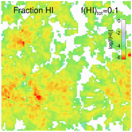
(g) $x_{\mathrm{H\,I,M}}$ at $z=6.49$.

(h) Photon density at $z=6.49$.

Figure 5: Maps of overdensity (a), redshift of reionization (b), ionizing photon emissivity (c,f), neutral hydrogen fraction (d,g), and the intensity of the ionizing background (e,h) in a volume slice $16h^{-1}{\rm Mpc}$ to a side and $250h^{-1}{\rm kpc}$ thick. Figures c–h are taken at two representative redshifts as indicated. The knots between filaments tend to host sources, but the filaments themselves have negligible emissivity, with the result that they reionize last (red color in panel b).

Figure 6: The ratio of the mass-weighted to volume-weighted ionized hydrogen fractions $x_{\mathrm{M}}/x_{\mathrm{V}}$ as a function of the age of the Universe (lower axis) and redshift (top axis). The top panels shows how $x_{\mathrm{M}}/x_{\mathrm{V}}$ drops more rapidly at higher spatial resolution owing to more efficient breakout of I-fronts into voids. We use polynomial fits to the simulated trends for $z\geq 9$. The inset panel shows the full simulated result for $\Delta x_{\mathrm{R}}=250h^{-1}{\rm kpc}$, where the jumps owe to the low time resolution in our set of precomputed density and emissivity fields. The bottom panel expands the y-axis from the top panel about $x_{\mathrm{M}}/x_{\mathrm{V}}=1$ in order to show how $x_{\mathrm{M}}/x_{\mathrm{V}}$ drops below unity well before reionization completes, with the effect growing stronger at higher resolution.

3.2 The Ratio of Ionized Fractions

Another way to study the topology of reionization is to consider the ratio of the mass-averaged to the volume-averaged ionized hydrogen fractions, $x_{\mathrm{M}}/x_{\mathrm{V}}$, which can be thought of as the average density of ionized regions in units of the mean density (Iliev et al., 2006a). For reionization in a homogeneous IGM, $x_{\mathrm{M}}/x_{\mathrm{V}}=1$ at all times. In an inhomogeneous IGM, OI reionization implies that $x_{\mathrm{M}}/x_{\mathrm{V}}\leq 1$ because ionizing voids increases $x_{\mathrm{H\,II,V}}$ more rapidly than $x_{\mathrm{H\,II,M}}$. Similarly, IO reionization implies that $x_{\mathrm{M}}/x_{\mathrm{V}}\geq 1$ because ionizing overdense regions increases $x_{\mathrm{H\,II,M}}$ more rapidly than $x_{\mathrm{H\,II,V}}$. In Figure 6, we show how $x_{\mathrm{M}}/x_{\mathrm{V}}$ evolves in time for three different choices of $\Delta x_{\mathrm{R}}$ in the radiation grid. For the period $z\geq 9$, we smooth the simulated results with cubic polynomial fits in order to suppress artifacts from low time resolution in our set of precomputed density and emissivity grids. The inset panel shows the original trend for the $\Delta x_{\mathrm{R}}=250h^{-1}{\rm kpc}$ calculation.

Broadly, $x_{\mathrm{M}}/x_{\mathrm{V}}$ evolves from $>1$ at early times when the ionized volume fraction remains low, to $<1$ when the voids reionize, to unity once the majority of the universe has reionized (see also Iliev et al., 2007). The early evolution is as expected if reionization begins earlier in overdense regions than in the Universe as a whole (Gnedin, 2000; Iliev et al., 2006a), but the tendency for $x_{\mathrm{M}}/x_{\mathrm{V}}$ to drop below unity significantly before reionization completes has not been discussed previously. The evolution of $x_{\mathrm{M}}/x_{\mathrm{V}}$ is sensitive to the choice of $\Delta x_{\mathrm{R}}$: Increasing spatial resolution increases $x_{\mathrm{M}}/x_{\mathrm{V}}$ at earlier times while decreasing it at late times. Physically, higher spatial resolution allows the simulation to better resolve the high recombination rates in the overdense regions where reionization begins, leading to more effective trapping of I-fronts at early times. At late times, increasing the resolution allows the simulation to resolve the tendency for I-fronts to “leak out” through the porous IGM into voids. As the bottom panel of Figure 6 indicates, this leaking effect is so efficient that, at our highest spatial resolution, $x_{\mathrm{M}}/x_{\mathrm{V}}$ drops below unity around the time when $x_{\mathrm{H\,I,V}}$ drops below 50% (at $z\approx 7$). In other words, by the time reionization is halfway complete, the average ionized region is underdense. This is a direct consequence of the late reionization of filaments.

3.3 The Mean Free Path of Ionizing Photons

The tendency of ionizing photons to stream preferentially in directions where the IGM is less dense naturally leads to the formation of ionized “tunnels” that connect sources with voids. If this tunnel formation indeed dominates the topology of reionization, and if the tunnels are small compared to $\Delta x_{\mathrm{R}}$, then the mean free path of ionizing photons $\lambda_{\mathrm{MFP}}$ from sources should increase with decreasing $\Delta x_{\mathrm{R}}$. This is because, as the tunnelling process is better-resolved, an increasing fraction of ionizing photons travel directly from sources through tunnels into voids rather than being artificially absorbed nearby. To test this idea, we have computed $\lambda_{\mathrm{MFP}}$ as a function of redshift by casting rays from each source (where a source is a computational cell with nonzero emissivity) in 1280 directions that uniformly sample the unit sphere and then computing the distance travelled until the optical depth exceeds 6. By repeating this exercise for each combination of $\Delta x_{\mathrm{R}}$ and redshift, we follow the growth of $\lambda_{\mathrm{MFP}}$ and its dependence on $\Delta x_{\mathrm{R}}$.

Figure 7: The ionizing mean free path $\lambda_{\mathrm{MFP}}$ from sources as a function of the volume-weighted ionized hydrogen fraction, computed using three different values of $\Delta x_{\mathrm{R}}$. The larger panel uses 6th-order polynomial fits to the simulated trends for $x_{\mathrm{H\,II,V}}<$10%, while the inset panel shows the full original curve for $\Delta x_{\mathrm{R}}=250h^{-1}{\rm kpc}$. At early times, higher resolution leads to higher $\lambda_{\mathrm{MFP}}$ because photons “tunnel” more effectively from sources to voids. At late times, higher spatial resolution leads to lower $\lambda_{\mathrm{MFP}}$ because the small overdensities that dominate the IGM opacity are better resolved.

We show the resulting trends of mean free path versus ionized volume fraction in Figure 7. During the early stages of reionization, when the neutral fraction is above 99%, higher resolution leads to higher $\lambda_{\mathrm{MFP}}$. This is the result that we expected: At higher spatial resolution, the tendency of photons to bore holes through the IGM from sources to voids is better resolved, leading to a higher $\lambda_{\mathrm{MFP}}$ at a given ionization state. In fact, Figure 7 indicates that even our highest-resolution computation does not fully capture all the relevant substructure, suggesting that the characteristic size of the tunnels is smaller than 250 comoving $h^{-1}{\rm kpc}$. It is likely that using a spatial resolution that is comparable to the virial radius of the dominant haloes is necessary for full resolution convergence. Unfortunately, this requirement is roughly a factor of 10 higher than what we have achieved here, and would require either a much smaller cosmological volume (thus increasing cosmic variance and biasing effects; Barkana & Loeb 2004), an adaptive RT mesh, or a less accurate technique. Nevertheless, the trend indicates that reionization proceeds rapidly from overdensities into voids before mopping up the filaments. It also reinforces the need for spatial resolutions that are much higher than 1 comoving $h^{-1}{\rm Mpc}$ when studying the topology of reionization.

As reionization proceeds, the trend of $\lambda_{\mathrm{MFP}}$ versus resolution inverts so that higher resolution leads to lower $\lambda_{\mathrm{MFP}}$. This occurs as the topology changes from one in which ionized tunnels thread an otherwise opaque IGM to one in which increasingly isolated overdensities are separated from each other by regions that are already reionized. The remaining neutral regions dominate the IGM opacity and shrink as reionization proceeds. Higher spatial resolution prevents them from being averaged with the low recombination rates in neighboring voids. At this stage, reionization proceeds from the voids back into regions of increasing density and decreasing spatial scale (Miralda-Escudé et al., 2000). Our simulations suggest that this topology could dominate by the time the neutral fraction drops below 50%, and possibly earlier.

4 Comparison to Observational Constraints

The goal of the present work is to take a hydrodynamical model that has enjoyed considerable success in accounting for observational constraints from the post-reionization Universe and to ask how reionization proceeds in this model. Because we have introduced no extra physical assumptions save for the choice of ionizing escape fraction and have tuned this to achieve reionization by $z=6$, it is of interest to compare our results with additional observational constraints from the reionization epoch, specifically Thomson optical depth measurements from the Wilkinson Microwave Anisotropy Probe (WMAP), and observations of the Lyman-$\alpha$ forest. In this Section we show that (1) our simulated optical depth to Thomson scattering underproduces the observed value and (2) our simulations overproduce the mean ionizing intensity at $z=6$. We discuss the implications of these findings.

4.1 The Integrated Optical Depth to Electron Scattering

Figure 8: The integrated optical depth to Thomson scattering $\tau_{\mathrm{es}}$ as a function of the age of the Universe (bottom axis) and redshift (top axis). Thick curves correspond to $\Delta x_{\mathrm{R}}=250h^{-1}{\rm kpc}$, $f_{\mathrm{esc}}=0.13$, and fiducial accuracy while thin curves correspond to $\Delta x_{\mathrm{R}}=500h^{-1}{\rm kpc}$, $f_{\mathrm{esc}}=1$, and the fast scheme (Section 2.2). Solid curves show the result from pure hydrogeon reionization, and dotted curves include the contribution of Helium assuming that Helium is doubly ionized after $z=3$ and singly ionized with $n_{\mathrm{He\,II}}/n_{\mathrm{He}}=n_{\mathrm{H\,II}}/n_{\mathrm{H}}$ for $z>3$. The dashed lines indicate the 68% confidence intervals for $\tau_{\mathrm{es}}$ arising from combining WMAP-5 with distance measurements from Type Ia supernovae and baryon acoustic oscillations, $\tau_{\mathrm{es}}=0.084\pm 0.016$ (Hinshaw et al., 2009; Komatsu et al., 2009). Our simulations do generate enough ionizing photons to match the observed constraint on $\tau_{\mathrm{es}}$, but our fiducial choice of $f_{\mathrm{esc}}$ may underproduce it.

In Figure 8, we show the variation of the integrated optical depth to Thomson scattering $\tau_{\mathrm{es}}$ with redshift. The thick solid curve corresponds to pure hydrogen reionization at our highest spatial resolution and accuracy, and indicates an integrated optical depth of 0.047, 0.023 below the 1-$\sigma$ observational constraints. Accounting for Helium reionization (thick dotted curve; see caption for details) boosts $\tau_{\mathrm{es}}$ to 0.051. The discrepancy between the observed and simulated $\tau_{\mathrm{es}}$, which reflects the history of the volume-averaged electron number density, suggests that reionization occurs too suddenly or too late in our calculations.

A number of effects could explain this discrepancy. On the numerical side, our hydrodynamic simulation may not resolve all of the relevant star formation at early times (Figure 2). Increased star formation at early times could start reionization earlier and boost $\tau_{\mathrm{es}}$ without changing $x_{\mathrm{H\,I,V}}$ at late times, when the ionizing background is dominated by more massive haloes (Figure 2; Iliev et al., 2007). The role of early star formation could be further enhanced through a more detailed treatment of the ionizing escape fraction, $f_{\mathrm{esc}}$. Currently, we have set $f_{\mathrm{esc}}$ to a time-invariant value of 13% in order to obtain the end of reionization at $z\approx 6$. However, this is a free parameter and could be larger at earlier times (e.g., Wise & Cen, 2009). Raising $f_{\mathrm{esc}}$ to 1 (thin curves) brings our simulated optical depth into agreement with the observed 68% confidence interval, but makes the redshift of overlap $z=7.90$. Note that this change slightly modifies the qualitative topology of reionization, but does not make it purely IO (Figure 9). Third, the finite spatial resolution affects $\tau_{\mathrm{es}}$ because reionization occurs more rapidly at higher $\Delta x_{\mathrm{R}}$ (see Section 3). For radiative transfer grid resolutions of $\Delta x=500,333,250h^{-1}{\rm kpc}$, $x_{\mathrm{H\,I,V}}$ drops below $10^{-3}$ at $z=$ 5.97, 6.05, and 6.20, respectively. Hence the choice of $\Delta x_{\mathrm{R}}$ introduces an uncertainty of approximately $\Delta z=$0.2. Finally, our small cosmological volume delays reionization by $\Delta z=0.1$ because of the lack of long-wavelength density fluctuations (Barkana & Loeb, 2004) and introduces a random uncertainty of $\Delta z=1$ owing to cosmic variance (Barkana & Loeb, 2004; Iliev et al., 2006a), which can be translated to an effect on $\tau_{\mathrm{es}}$ via $d\tau_{\mathrm{es}}/dz_{\mathrm{reion}}\approx 0.008$. In short, the systematic uncertainties in our reionization history owing to numerical effects and assumptions are sufficient to account for the missing optical depth.

But there are further observational uncertainties related to the observed $\tau_{\mathrm{es}}$.  Shull & Venkatesan (2008) have argued that the systematic uncertainties in computing the residual electron fraction leftover after recombination lead to systematic uncertainties in $\tau_{\mathrm{es}}$ of order $\sim 0.01$. If true, then this could reduce the amount of Thomson scattering that galaxies are responsible for producing, bringing our simulations into better agreement with observations. The unknown time dependence of reionization also renders $\tau_{\mathrm{es}}$ uncertain (although Mortonson & Hu 2008 have argued that realistic reionization histories systematically increase $\tau_{\mathrm{es}}$ over the instantaneous reionization value, which would further increase the discrepancy with our simulations).

Finally, it is also possible that reproducing $\tau_{\mathrm{es}}$ in large cosmological volumes requires additional physical processes such as self-regulation of star formation in low mass haloes (Iliev et al., 2007), Population III stars (Trac & Cen, 2007; Shin et al., 2008), X-rays from early black holes (Shull & Venkatesan, 2008) or supernovae (Oh, 2001), or primordial magnetic fields (Schleicher et al., 2008). In future work, we will use radiative hydrodynamic simulations of reionization to study self-regulation; however, for the present, our goal is to study how reionization follows from our existing baryonic physics treatments with no additional assumptions.

4.2 The Hydrogen Ionization Rate at $z=6$

The solid blue curve in the bottom panel of Figure 3 shows how the volume-averaged hydrogen ionization rate per hydrogen atom $\Gamma_{-12}\equiv\Gamma_{\mathrm{H\,I}}/10^{-12}$ varies with redshift in our calculation. At $z=6$, we find $\log(\Gamma_{-12})=1$, whereas observations of the Lyman-$\alpha$ forest indicate $\log(\Gamma_{-12})<-0.6$ (triangle with arrow; Bolton & Haehnelt, 2007; Srbinovsky & Wyithe, 2008). Relatedly, our fiducial simulation yields a volume-averaged neutral fraction at $z=6$ of $2.4\times 10^{-6}$, 50–100 times smaller than the observed 2–3$\times 10^{-4}$ (Fan et al., 2006).

These large discrepancies could result either from $f_{\mathrm{esc}}$ being too high or from the opacity in the reionized IGM being too low. The fact that reionization occurs more rapidly at higher spatial resolution (Figure 4) indicates that we are forced to choose $f_{\mathrm{esc}}$ artificially large in order to achieve overlap by $z=6$. Meanwhile, the fact that the IGM opacity at a given ionization state increases with decreasing $\Delta x_{\mathrm{R}}$ (Figure 7) indicates that our simulated IGM opacity at $z=6$ is artificially low. Both of these effects indicate that increasing our spatial resolution or incorporating a subgrid treatment for photoionization of structures below our spatial resolution (e.g., Ciardi et al., 2006; Trac & Cen, 2007) would improve the agreement with the observed $\Gamma_{-12}$.

We may estimate how much our $\Gamma_{-12}$ would improve with resolution by considering the likely impact of structures below our spatial resolution. Under ionization equilibrium, the emissivity and ionization rate are related by

$$\eta=\chi\Gamma/4\pi\sigma.$$ (1)

Here, $\eta=2.694\times 10^{-24}(f_{\mathrm{esc}}/0.13)$ is our simulated volume-averaged comoving emissivity at $z=6$ in s^-1 cm^-3 Sr^-1; $\chi$ is the opacity to ionizing photons in cm^-1; and $\sigma$ is the neutral hydrogen cross section at the Lyman limit in cm^-2. At $z=6$, the IGM opacity is dominated by Lyman limit systems, hence we may approximate $\chi$ as the reciprocal of the mean free path to Lyman limit systems. Extrapolating the number density found by Storrie-Lombardi et al. (1994), this is 84 comoving Mpc in our cosmology at $z=6$. Faucher-Giguère et al. (2008) have estimated the additional impact of structures at lower column densities, finding that the mean free path is roughly $85[(1+z)/4]^{-4}$ proper Mpc (or 63 comoving Mpc at $z=6$). Folding these estimates into Equation 1, we find that resolving Lyman limit systems could reduce $\Gamma_{-12}$ from $\approx 10$ to 2. This is still larger than the observed upper limit of 0.3 (Bolton & Haehnelt, 2007; Srbinovsky & Wyithe, 2008), suggesting that our escape fraction may still be too large. However, given that increasing the spatial resolution also accelerates reionization (Figure 4), this observation reinforces our previous conclusion that decreasing both $\Delta x_{\mathrm{R}}$ and $f_{\mathrm{esc}}$ without changing our star formation prescription would yield improved agreement with the observations.

Of course, while it is possible that these discrepancies owe to a combination of numerical effects and systematic uncertainties in the observed optical depth to Thomson scattering, a more interesting possibility is that they indicate a failing of the input physics. For example, detailed comparisons with observations of galaxies and the IGM in the post-reionization Universe have prompted us to assume that low-mass galaxies generate strong outflows (Section 1). These outflows dramatically suppress the ionizing emissivity at early times, leading to a relatively late reionization epoch and a low $\tau_{\mathrm{es}}$. As a reference point, in our simulations, 90% of the ionizing photons that are emitted by $z=6$ are emitted after $z=9$. Weaker outflows at early times would boost early star formation rates and hence $\tau_{\mathrm{es}}$. A stronger scaling between ionizing luminosity and metallicity over what is found in the Bruzual & Charlot (2003) models would enhance the ionizing light to mass ratios, as would including a treatment for an evolving initial mass function (i.e., Population III star formation), or the inclusion of mini-quasars. Finally, an ionizing escape fraction that decreases with decreasing redshift or increasing halo mass would enhance the ionizing luminosity into the IGM without changing the star formation history. However, until the numerical issues are more fully investigated, we cannot make robust conclusions about the need for new or enhanced sources of ionizing photons at the earliest epochs.

In summary, the failure of our simulations to reproduce simultaneously the observed optical depth to Thomson scattering and the hydrogen ionization rate at $z=6$ could owe to observational uncertainties, numerical effects, or inadequate physics treatments. On the other hand, given that our simulations have previously been shown to reproduce a wide variety of observations of the post-reionization Universe and that the only additional physical assumption that we have introduced is the choice of ionizing escape fraction, the level of agreement that we find is encouraging. Our results support the idea that the processes governing star formation before and after reionization may not have been very different (Davé et al., 2006).

5 Discussion

The tendency for I-fronts to bypass filaments and escape directly into voids occurs generically in calculations that assume static emissivity and density fields (as we did in Finlator et al. 2009). Given high enough spatial resolution, such calculations invariably produce H II regions with “butterfly wing” morphologies (e.g., Ciardi et al., 2001; Iliev et al., 2006b; Tasitsiomi, 2006). In addition, this effect has recently been found in radiative hydrodynamic simulations of the first stages of star formation (Abel et al., 2007; Wise & Abel, 2008). This was on much smaller scales ($<1h^{-1}{\rm Mpc}$) than the cosmological scales that we are interested in. Nonetheless, one may understand the result in both cases as a competition between the timescale for photons to bore tunnels through the IGM that connect sources with voids on the one hand versus the timescale for filaments to self-ionize and the timescale for I-fronts to burn directly through filaments on the other. If photons leak into voids more rapidly than the filaments can either be ionized or self-ionize, then the voids will reionize before the filaments.

These timescales are in turn governed by three factors: (1) The emissivity field’s bias with respect to the baryon density field; (2) the time evolution of the emissivity field; and (3) the spatial resolution. The impact of the emissivity bias on the topology of reionization has been explored elsewhere (McQuinn et al., 2007); for our purposes it suffices to note that a highly biased emissivity field promotes the late reionization of filaments by preventing them from self-ionizing. The time evolution of the ionizing emissivity matters because if the emissivity is relatively high at early times, then the late reionization of filaments is suppressed even in the presence of a biased emissivity field owing to the lower density contrast in the IGM. As a demonstration of this effect, we show the reionization topology resulting from setting $f_{\mathrm{esc}}=1$ in Figure 9 (cyan dot-dashed curve). Comparing this curve to the topology in our fiducial case (solid black curve) reveals that the higher reionization redshift is indeed associated with a flatter trend of median reionization redshift versus overdensity at low densities. Finally, high spatial resolution also promotes the early reionization of voids by increasing the density contrast. The topology presented in this paper results from a particular combination of emissivity bias and evolution that has not been considered previously, and it is most clearly visible only at our highest spatial resolution (Figure 6).

Iliev et al. (2006a) ran post-processed radiative transfer calculations of cosmological reionization on snapshots obtained from a pure N-body simulation. In contrast to our results, they found a purely IO topology. Given that their spatial resolution was comparable to ours, the difference between our results must owe to the different emissivity fields. In constructing their emissivity field, they considered only haloes more massive than $2.5\times 10^{9}M_{\odot}$, which implies an even more biased emissivity field than ours (Figure 2). Choudhury et al. (2009) suggested that their purely IO topology might result from using high emissivities. Indeed, the Iliev et al. (2006a) simulation achieved reionization by $z\sim 11$, only $\approx 260$ Myr after the first sources formed at $z=21$, whereas our simulations are tuned to produce reionization at $z=6$, roughly 680 Myr after the computations begin at $z=14$. We conclude that their purely IO topology owed to their high reionization redshift and the resulting lower IGM density contrast.

Subsequent calculations involving more extended reionization histories and lower overlap redshifts have also resulted in more nearly IO-like topologies (Trac & Cen, 2007; Iliev et al., 2007), hence the overlap redshift alone is not the only cause of our topology. In the case of Trac & Cen (2007), we ascribe the difference to our more biased emissivity field. For example, comparing our Figure 2 with their Figure 1, we find that, at $z=6$, the minimum halo mass above which 60% of ionizing photons are emitted is $10^{9.4}M_{\odot}$ for our simulation versus $10^{9}M_{\odot}$ for theirs. Their more extended reionization history also allows for much of reionization to take place at higher redshift, when density contrasts are lower. Our less gradual reionization history owes directly to our star formation prescription, which suppresses the early star formation rate density with respect to models that do not include strong outflows (e.g., Figure 3 of Oppenheimer & Davé 2006) and leads to a more sudden overlap epoch because of the strong dependence of star formation rate on halo mass (Figure 1).

The emissivity field of Iliev et al. (2007) is also less biased than ours, but this time in two respects. First, they assume that haloes with masses between $10^{8\mbox{--}9}M_{\odot}$ are the sites of Population III star formation, leading to lower ratios of mass to ionizing luminosity than more massive haloes. Second, they assume that the ionizing luminosity is proportional to halo mass, which, even in the absence of Population III stars, would yield a less-biased emissivity field than ours since our ionizing luminosity scales as $M^{1.3}$ (Figure 1). With these assumptions, it is not surprising that their filaments are able to self-ionize much more efficiently than ours.

Figure 9: Systematic effects on the median reionization redshift as a function of overdensity. The horizontal segments on the right indicate the corresponding overlap redshifts. Short-dashed blue, solid black, and long-dashed red curves show the results assuming three different values $c^{\prime}$ for the speed of light. The dotted green curve shows the results when the emissivity is derived from the star formation rates. The dot-dashed magenta curve uses a cosmological volume eight times as large as our fiducial volume. Because these computations used somewhat less accurate Eddington tensors in order to save time, we also include the result at our fiducial accuracy (light grey curves). Changing the speed of light or the volume does not qualitatively change the topology of reionization, but it does impact the overlap redshift. Changing how we derive the emissivity field does not affect our results either.

The simulations of Iliev et al. (2007, 2006a) assume that the speed of light is infinite whereas ours do not; could this assumption impact the topology of reionization? As this question has not been investigated in a fully numerical context previously, we have re-computed cosmological reionization using $\Delta x_{\mathrm{R}}=500h^{-1}{\rm kpc}$ assuming three different values $c^{\prime}$ for the speed of light: $c/10$, $c$, and $10c$. To save time, we perform these integrations using our less-accurate “fast” scheme for updating the Eddington tensors (Section 2.2). Figure 9 shows how the trend of median redshift of reionization versus overdensity (curves) and the overlap redshift (horizontal lines) vary with the speed of light. The light solid curve reflects our fiducial accuracy and is copied from Figure 4. It essentially overlaps the dark solid curve, indicating that the impact of the somewhat less accurate Eddington tensors in our fast scheme is small compared to the systematic offset from using an inaccurate speed of light. The median redshift of reionization is roughly $\Delta z=0.1$ (50 Myr) earlier at all densities for $c^{\prime}=10c$ and 0.2–0.4 (150 Myr) later for $c^{\prime}=c/10$, although in both cases the effects are stronger in the underdense than in the overdense regions. Overlap (defined as the redshift when $x_{\mathrm{H\,I,V}}$ drops below $10^{-3}$) occurs $\Delta z=(0.3,0.6)$ or (50,150) Myr (early, late) for $c^{\prime}=(10c,c/10)$. Evidently, the consequences of decreasing the speed of light (as done by e.g. Aubert & Teyssier, 2008) are more dramatic than the consequences of boosting it, although neither approximation changes the qualitative topology of reionization.

McQuinn et al. (2007) investigated a variety of emissivity fields, including cases that were much more biased than ours (their models S3 and S4). Although they did not specifically address the onset of OI reionization, we may speculate on whether their results would have agreed with ours. Their fiducial model S1 corresponds to a less biased field than ours partly because it includes the contribution of all haloes down to $10^{8}M_{\odot}$, and partly because they assume a constant mass-to-light ratio. Their model S3 includes a stronger scaling between halo mass and luminosity than we find, but it still includes the contribution of the low-mass ($<10^{8.5}M_{\odot}$) haloes. Their model S4 assumes that haloes with masses below $4\times 10^{10}M_{\odot}$ do not form stars, hence it corresponds to an extremely biased emissivity field. However, because they tune the emissivities to match the volume-averaged emissivity in their S1 model, reionization is already well underway before the density contrasts are large enough for the filaments to self-shield efficiently. Hence, of their models, the S3 would have been the most similar to ours. Unfortunately, their spatial resolution is slightly lower than ours ($367h^{-1}{\rm kpc}$ versus $250h^{-1}{\rm kpc}$), which artificially suppresses the density contrast and hence the onset of the OI phase (Figure 6).

It is possible that increasing our mass resolution would boost the star formation rates in low mass haloes at early times, leading to a less biased emissivity and more extended reionization history. However, even in this case our results would remain sensitive to the unknown ionizing escape fraction, which may decrease with decreasing mass (Gnedin et al., 2008; Wise & Cen, 2009) or increasing gas fraction (Oey et al., 2007). Our finding that the topology of reionization depends sensitively on assumptions regarding baryonic physics in low-mass haloes emphasizes the need for improved observational constraints on the faint end of the luminosity function as well as on the escape fraction of ionizing photons. It also emphasizes the need for high-resolution radiative hydrodynamic simulations of galaxy formation during the reionization epoch (e.g. Wise & Cen, 2009) in order to tune the assumptions that go into larger-scale simulations.

Our limited cosmological volume may introduce some uncertainty into our results. It has been shown that the lack of long-wavelength density fluctuations sampled by our $16h^{-1}{\rm Mpc}$ volume delays overlap by $\Delta z=0.1$ and introduces an uncertainty of $\Delta z=1$ owing to cosmic variance (e.g., Barkana & Loeb, 2004; Iliev et al., 2006a). While it has not been shown that these effects qualitatively change the topology of reionization, we have explored this possibility by computing reionization using snapshots extracted from a $32h^{-1}{\rm Mpc}$ cosmological hydrodynamic simulation. The baryonic physics treatments in this simulation are the same as in our fiducial volume, as is the assumed ionizing escape fraction. Its spatial resolution is $8\times$ lower, with the result that star formation is artificially suppressed in haloes below the 64-particle limit of $1.5\times 10^{9}M_{\odot}$. We use a grid of $64^{3}$ cells, making $\Delta x_{\mathrm{R}}$ identical to the tests in Figure 9. The dot-dashed magenta curve in Figure 9 shows the resulting reionization topology. Comparing it to the solid black curve, we find that the topology is qualitatively unchanged. In detail, overdense regions reionize later owing to the delay of star formation at lower mass resolution (e.g., Springel & Hernquist, 2003b). This in turn delays the overlap epoch by roughly $\Delta z=0.2$. Ideally, we would prefer run this test on outputs from an even larger hydrodynamic simulation that used the same mass resolution. Unfortunately, this is not possible with our current computing resources. Nevertheless, the qualitative agreement between our $16h^{-1}{\rm Mpc}$ and $32h^{-1}{\rm Mpc}$ volumes suggests both that our topology does not owe to cosmic variance, and that using an even larger volume would not change our results. It would be interesting to compute the reionization of a $16h^{-1}{\rm Mpc}$ or $32h^{-1}{\rm Mpc}$ volume using a testbed that is known to yield a purely inside-out reionization topology for larger volumes; however, this is beyond the scope of our present work.

An additional source of uncertainty in our results is the unknown impact of structures on size scales below our spatial resolution such as virialized haloes with masses in the range $10^{5\mbox{--}7}M_{\odot}$ (i.e., minihaloes). Given that the timescale for ionizing photons to bore holes through the IGM into the voids is comparable to the timescale over which the Universe emits enough photons to ionize each baryon once, minihaloes—which are concentrated in filaments—could tilt the competition further in favor of an IOM topology through their ability to delay the completion of reionization by up to $\Delta z=2$ (e.g., Barkana & Loeb, 2002; Ciardi et al., 2006; McQuinn et al., 2007). Moreover, analytic and numerical studies now agree that minihaloes change the topology of reionization, decreasing the number of large H II regions and increasing the number of small ones (McQuinn et al., 2007; Furlanetto & Oh, 2005) at late times. Although we do not actually resolve minihaloes, this finding is completely consistent with the trend that we found in Figure 7 whereby the mean free path to ionizing photons in the latter stages of reionization is shorter at higher spatial resolution owing to the impact of overdense “holdouts”. This, however, is in the late stages of reionization ($x_{\mathrm{H\,II,V}}>0.5$); what about during the early stages? Minihaloes cannot substantially affect the topology of reionization until the mean free path to absorption by the IGM is comparable to mean free path to pass within a virial radius of a minihalo, which, for a Press-Schechter mass function and our reionization history, happens after $z=8$. By contrast, Figure 3 indicates that the strength of the ionizing background in voids is already comparable to the volume average by $z=9$. We conclude that minihaloes are not likely to prevent the IOM topology because they are not numerous enough to obstruct the photons’ paths into the voids.

6 Summary

We have used our new moment-based radiative transfer technique to study how cosmological reionization proceeds on precomputed grids of density and ionizing emissivity spanning a $16^{3}h^{-3}$ Mpc³ volume. We extract these grids from a cosmological hydrodynamic simulation that resolves all star formation in dark matter haloes more massive than $2\times 10^{8}M_{\odot}$. This mass threshold accounts for most of the relevant star formation prior to the onset of reionization and all of it once reionization is well underway since the nascent ionizing background suppresses star formation in haloes less massive than $\sim 10^{9}M_{\odot}$.

We find that reionization proceeds rapidly from overdense regions into voids owing to the porous nature of the IGM, with filamentary structures ionizing last, which we call an inside-outside-middle (IOM) topology. This is consistent with what we obtained previously using less sophisticated methods (Finlator et al., 2009). In our models this IOM topology arises because filaments cannot self-ionize, since haloes less massive than $\sim$a few$\times 10^{8}M_{\odot}$ do not form stars efficiently. While this cutoff may owe to resolution limitations in our simulation prior to the onset of reionization, it is an expected consequence of Jeans mass suppression in reionized regions and the primordial cooling floor at $10^{4}$ K.

The mean density of ionized regions $x_{\mathrm{M}}/x_{\mathrm{V}}$ drops from high values at early times to the cosmological mean density following the epoch of overlap, as expected given that sources lie predominantly in overdense regions. At higher spatial resolution, the tendency for photons to “leak” directly into voids suppresses $x_{\mathrm{M}}/x_{\mathrm{V}}$ more rapidly so that, at our highest resolution, the mean density of ionized regions drops below the cosmological mean density once the volume-averaged ionized hydrogen fraction $x_{\mathrm{H\,II,V}}$ surpasses 50%. This leaking effect also manifests as a tendency for the mean free path for ionizing photons $\lambda_{\mathrm{MFP}}$ to increase at higher spatial resolution for $x_{\mathrm{H\,II,V}}<10$%. At later stages, $\lambda_{\mathrm{MFP}}$ decreases at higher resolution because the dense condensations that dominate the IGM opacity at late times are better resolved.

Our reionization history underpredicts the integrated optical depth to Thomson scattering and overpredicts the strength of the ionizing background at $z=6$. The low optical depth could indicate that reionization begins too late and that $f_{\mathrm{esc}}$ should be increased, while the high ionizing background suggests that the IGM opacity at $z=6$ is too low. Increasing $f_{\mathrm{esc}}$ to unity leads to better agreement with the observed optical depth while exacerbating the discrepancy with the observed ionizing background at $z=6$. An interesting alternative would be to have $f_{\mathrm{esc}}=1$ for small haloes while leaving it at $\leq 10$% for larger haloes. This would increase the electron fraction at early times, when the ionizing background is dominated by low-mass haloes, while leaving it unchanged at late times, when the haloes below $5\times 10^{8}M_{\odot}$ no longer form stars. This would be analogous to models considering Population III star formation and self-regulation of star formation in low-mass haloes, which have been shown to yield good agreement with WMAP observations (Iliev et al., 2007).

The qualitative topology of reionization is robust to our choice of spatial resolution, cosmological volume, and ionizing escape fraction even though each of these affects the overlap redshift. Increasing the spatial resolution delays reionization in overdense regions owing to more effective I-front trapping while advancing the reionization of voids owing to more efficient “tunneling” of photons through small-scale soft spots in the IGM. The latter effect also causes overlap to occur sooner. Doubling the length of our simulation volume from $16$ to $32h^{-1}{\rm Mpc}$ delays overlap by $\Delta z\approx 0.1$ because the delayed onset of star formation at lower mass resolution wins over the tendency for overlap to occur earlier in larger periodic volumes. The topology, however, remains essentially unchanged. Increasing the ionizing escape fraction to unity causes overlap to occur sooner by $\Delta z\approx 2$. Additionally, although the filaments are still the last regions to ionize in this scenario, they do so somewhat sooner with respect to the voids owing to the decreased density contrast at higher redshift. This suggests that enhancing the ionizing emissivity at early times by, for example, increasing the ionizing escape fraction from low-mass halos would lead to a more IO-like topology.

We have also explored how approximations regarding the speed of light and the accuracy of the Eddington tensors impact reionization. Broadly, we find that, while these approximations do not qualitatively change the topology of reionization, they do affect the overlap redshift. We find that (increasing/decreasing) the speed of light by a factor of 10 (advances/delays) overlap by (50/150) Myr or $\Delta z=$ (0.3/0.6). At a resolution of $\Delta x_{\mathrm{R}}=250h^{-1}{\rm kpc}$, using Eddington tensors derived in the optically thin limit delays reionization by 40 Myr or $\Delta z=0.2$, primarily by delaying the reionization of filaments. These results emphasize the need to avoid such physical approximations when an accurate calculation of reionization is desired, and also highlight an important feature of our accurate RT code that enables us to directly check the impact of such approximations.

Simulations of reionization are in their infancy. Ideally, one would like a single model to span first stars calculations on sub-kpc scales within cosmological volumes that encompass the largest ionization bubbles at overlap. Our current codes cannot do so, but future improvements such as an adaptive RT mesh and its incorporation into the hydrodynamical evolution will bring us closer to this goal. Meanwhile, we can still gain key insights into the topology of reionization, and better understand how one must compute reionization accurately. This will set the framework for understanding the rapidly advancing observations of this final cosmic frontier.

References

- Abel et al. (2007) Abel, T., Wise, J. H., & Bryan, G. L. 2007, ApJL, 659, L87
- Ahn et al. (2009) Ahn, K., Shapiro, P. R., Iliev, I. T., Mellema, G., & Pen, U.-L. 2009, ApJ, 695, 1430
- Aubert & Teyssier (2008) Aubert, D., & Teyssier, R. 2008, MNRAS, 387, 295
- Barkana & Loeb (2002) Barkana, R., & Loeb, A. 2002, ApJ, 578, 1
- Barkana & Loeb (2004) Barkana, R., & Loeb, A. 2004, ApJ, 609, 474
- Bolton & Haehnelt (2007) Bolton, J. S., & Haehnelt, M. G. 2007, MNRAS, 382, 325
- Bouwens et al. (2007) Bouwens, R. J., Illingworth, G. D., Franx, M., & Ford, H. 2007, ApJ, 670, 928
- Bruzual & Charlot (2003) Bruzual, G. & Charlot, S. 2003, MNRAS, 344, 1000
- Chabrier (2003) Chabrier, G. 2003, PASP, 115, 763
- Choudhury et al. (2009) Choudhury, T. R., Haehnelt, M. G., & Regan, J. 2009, MNRAS, 394, 960
- Ciardi et al. (2001) Ciardi, B., Ferrara, A., Marri, S., & Raimondo, G. 2001, MNRAS, 324, 381
- Ciardi et al. (2006) Ciardi, B., Scannapieco, E., Stoehr, F., Ferrara, A., Iliev, I. T., & Shapiro, P. R. 2006, MNRAS, 366, 689
- Davé et al. (2006) Davé, R., Finlator, K., & Oppenheimer, B. D. 2006, MNRAS, 370, 273
- Davé et al. (2008) Davé, R., Oppenheimer, B. D., & Sivanandam, S. 2008, MNRAS, 391, 110
- Fan et al. (2006) Fan, X., et al. 2006, AJ, 132, 117
- Faucher-Giguère et al. (2008) Faucher-Giguère, C.-A., Lidz, A., Hernquist, L., & Zaldarriaga, M. 2008, ApJ, 688, 85
- Finlator & Davé (2008) Finlator, K., & Davé, R. 2008, MNRAS, 385, 2181
- Finlator et al. (2009) Finlator, K., Özel, F., & Davé, R. 2009, MNRAS, 393, 1090
- Finlator et al. (2007) Finlator, K., Davé, R., & Oppenheimer, B. D. 2007, MNRAS, 376, 1861
- Furlanetto & Oh (2005) Furlanetto, S. R., & Oh, S. P. 2005, MNRAS, 363, 1031
- Gnedin & Ostriker (1997) Gnedin, N. Y., & Ostriker, J. P. 1997, ApJ, 486, 581
- Gnedin (2000) Gnedin, N. Y. 2000, ApJ, 535, 530
- Gnedin et al. (2008) Gnedin, N. Y., Kravtsov, A. V., & Chen, H.-W. 2008, ApJ, 672, 765
- Haiman et al. (1997) Haiman, Z., Rees, M. J., & Loeb, A. 1997, ApJ, 476, 458
- Haardt & Madau (2001) Haardt, F. & Madau, P. 2001, in proc. XXXVIth Rencontres de Moriond, eds. D.M. Neumann & J.T.T. Van.
- Hinshaw et al. (2009) Hinshaw, G., et al. 2009, ApJS, 180, 225
- Iliev et al. (2006a) Iliev, I. T., Mellema, G., Pen, U.-L., Merz, H., Shapiro, P. R., & Alvarez, M. A. 2006, MNRAS, 369, 1625
- Iliev et al. (2006b) Iliev, I. T., et al. 2006, MNRAS, 371, 1057
- Iliev et al. (2007) Iliev, I. T., Mellema, G., Shapiro, P. R., & Pen, U.-L. 2007, MNRAS, 376, 534
- Kennicutt (1998a) Kennicutt, R. C. 1998, ApJ, 498, 541
- Kennicutt (1998a) Kennicutt, R. C., Jr. 1998, ARA&A, 36, 189
- Komatsu et al. (2009) Komatsu, E., et al. 2009, ApJS, 180, 330
- Lee et al. (2008) Lee, K.-G., Cen, R., Gott, J. R. I., & Trac, H. 2008, ApJ, 675, 8
- Lidz et al. (2009) Lidz, A., Zahn, O., Furlanetto, S. R., McQuinn, M., Hernquist, L., & Zaldarriaga, M. 2009, ApJ, 690, 252
- McKee & Ostriker (1977) McKee, C. F. & Ostriker, J. P. 1977, ApJ, 218, 148
- McQuinn et al. (2007) McQuinn, M., Lidz, A., Zahn, O., Dutta, S., Hernquist, L., & Zaldarriaga, M. 2007, MNRAS, 377, 1043
- Miralda-Escudé et al. (2000) Miralda-Escudé, J., Haehnelt, M., & Rees, M. J. 2000, ApJ, 530, 1
- Mortonson & Hu (2008) Mortonson, M. J., & Hu, W. 2008, ApJL, 686, L53
- Nakamoto et al. (2001) Nakamoto, T., Umemura, M., & Susa, H. 2001, MNRAS, 321, 593
- Oey et al. (2007) Oey, M. S., et al. 2007, ApJ, 661, 801
- Oh (2001) Oh, S. P. 2001, ApJ, 553, 499
- Okamoto et al. (2008) Okamoto, T., Gao, L., & Theuns, T. 2008, MNRAS, 390, 920
- Oppenheimer & Davé (2006) Oppenheimer, B. D., & Davé, R. 2006, MNRAS, 373, 1265
- Oppenheimer & Davé (2008) Oppenheimer, B. D., & Davé, R. 2008, MNRAS, 387, 577
- Oppenheimer et al. (2009) Oppenheimer, B. D., Davé, R., & Finlator, K. 2009, MNRAS, 396, 729
- Schleicher et al. (2008) Schleicher, D. R. G., Banerjee, R., & Klessen, R. S. 2008, PhRvD, 78, 083005
- Shin et al. (2008) Shin, M.-S., Trac, H., & Cen, R. 2008, ApJ, 681, 756
- Shull & Venkatesan (2008) Shull, J. M., & Venkatesan, A. 2008, ApJ, 685, 1
- Sutherland & Dopita (1993) Sutherland, R. S. & Dopita, M. A. 1993, ApJS, 88, 253
- Springel & Hernquist (2002) Springel, V. & Hernquist, L. 2002, MNRAS, 333, 649
- Springel & Hernquist (2003a) Springel, V. & Hernquist, L. 2003a, MNRAS, 339, 289
- Springel & Hernquist (2003b) Springel, V., & Hernquist, L. 2003, MNRAS, 339, 312
- Srbinovsky & Wyithe (2008) Srbinovsky, J., & Wyithe, S. 2008, arXiv:0807.4782
- Storrie-Lombardi et al. (1994) Storrie-Lombardi, L. J., McMahon, R. G., Irwin, M. J., & Hazard, C. 1994, ApJL, 427, L13
- Tasitsiomi (2006) Tasitsiomi, A. 2006, ApJ, 645, 792
- Thoul & Weinberg (1996) Thoul, A. A., & Weinberg, D. H. 1996, ApJ, 465, 608
- Trac & Cen (2007) Trac, H., & Cen, R. 2007, ApJ, 671, 1
- Trac et al. (2008) Trac, H., Cen, R., & Loeb, A. 2008, ApJL, 689, L81
- Wise & Cen (2009) Wise, J. H., & Cen, R. 2009, ApJ, 693, 984
- Wise & Abel (2008) Wise, J. H., & Abel, T. 2008, ApJ, 684, 1