Evolution of the cosmological mass density of neutral gas from Sloan Digital Sky Survey II - Data Release 7

We present the results of a search for damped Lyman-$\alpha$ (DLA) systems in the Sloan Digital Sky Survey II (SDSS), Data Release 7. We use a fully automatic procedure to identify DLAs and derive their column densities. The procedure is checked against the results of previous searches for DLAs in SDSS. We discuss the agreements and differences and show the robustness of our procedure. For each system, we obtain an accurate measurement of the absorber’s redshift, the H i column density and the equivalent width of associated metal absorption lines, without any human intervention. We find 1426 absorbers with $2.15<z<5.2$ with $\log N({H\textsc{i}})\geq 20$, out of which 937 systems have $\log N({H\textsc{i}})\geq 20.3$. This is the largest DLA sample ever built, made available to the scientific community through the electronic version of this paper.

In the course of the survey, we discovered the intervening DLA with highest H i column density known to date with $\log N({H\textsc{i}})=22.0\pm 0.1$. This single system provides a strong constraint on the high-end of the $N({H\textsc{i}})$ frequency distribution now measured with high accuracy.

We show that the presence of a DLA at the blue end of a QSO spectrum can lead to important systematic errors and propose a method to avoid them. This has important consequences for the measurement of the cosmological mass density of neutral gas at $z\sim 2.2$ and therefore on our understanding of galaxy evolution over the past 10 billion years.

We find a significant decrease of the cosmological mass density of neutral gas in DLAs, $\Omega_{\rm g}^{\rm DLA}$, from $z=4$ to $z=2.2$, consistent with the result of previous SDSS studies. However, and contrary to other SDSS studies, we find that $\Omega_{\rm g}^{\rm DLA}(z=2.2)$ is about twice the value at $z=0$. This implies that $\Omega_{\rm g}^{\rm DLA}$ keeps decreasing at $z<2.2$.

1 Introduction

Despite accounting for only a small fraction of all the baryons in the Universe (see Fukugita & Peebles, 2004), the neutral and molecular phases of the interstellar medium are at any redshift the reservoir of gas from which stars form. Therefore, determining the cosmological mass density of neutral gas ($\Omega_{\rm HI}$) and its evolution in time is a fundamental step forward towards understanding how galaxies form (Klypin et al., 1995).

In the local Universe, neutral gas is best traced by the hyperfine 21-cm emission of atomic hydrogen. Its observation allows for an accurate measurement of the neutral gas spatial distribution in nearby galaxies and strongly constrains the column density frequency distribution (Zwaan et al., 2005b) and $\Omega_{{H\textsc{i}}}(z=0)$ (Zwaan et al., 2005a). However, the limited sensitivity of current radio telescopes prevents direct detections of H i emission beyond $z\sim 0.2$ (Lah et al., 2007; Verheijen et al., 2007; Catinella et al., 2008).

At high redshift, most of the neutral hydrogen is revealed by the Damped Lyman-$\alpha$ (DLA) absorption systems detected in the spectra of background quasars. While most of the gas is likely to be neutral for $\log N({H\textsc{i}})>19.5$ (Viegas, 1995), the conventional definition for Damped Lyman-$\alpha$ systems is $\log N({H\textsc{i}})\geq 20.3$ (Wolfe et al., 1986). Not only does this correspond to a convenient detectability limit in low-resolution spectra, but also to a critical surface-density limit for star formation. Since DLAs are easy to detect and the H i column densities can be measured accurately, it is possible to measure the cosmological mass density of neutral gas at different redshifts, independently of the exact nature of the absorbers, provided a sufficiently large number of background quasars is observed. However, any bias affecting the selection of the quasars or the determination of the redshift path-length probed by each line of sight can affect the measurements.

The Lick survey, the first systematic search for DLAs, led to the detection of 15 systems at $\left<z\right>=2.5$ along the line of sight to 68 quasars (Wolfe et al., 1986; Turnshek et al., 1989; Wolfe et al., 1993). About one hundred quasars were subsequently surveyed for DLA absorptions by Lanzetta et al. (1991). A number of surveys have followed (e.g. Wolfe et al., 1995; Lanzetta et al., 1995; Storrie-Lombardi et al., 1996a, b; Storrie-Lombardi & Wolfe, 2000; Ellison et al., 2001; Péroux et al., 2003; Rao et al., 2005, 2006), each of them contributing significantly to increase the number of known DLAs and the redshift coverage. On the other hand, surveys at low and intermediate redshifts are difficult because they require UV observations and the number of confirmed systems is building up very slowly (Lanzetta et al., 1995; Rao et al., 2005, 2006).

In turn, Péroux et al. (2001, 2003) aimed at the highest redshifts by observing 66 quasars with $z_{\rm em}>4$. They included data from previous surveys in their analysis, which led to the largest DLA sample available at that time. They found no significant evolution of the cosmological mass density of neutral gas over the redshift range $1<z<4$ and suggested that a significant part of this mass is due to systems with neutral hydrogen column densities below the conventional DLA cutoff limit.

The most recent contribution to the actual census of DLAs is a semi-automatic data mining of thousands of quasar spectra from the Sloan Digital Sky Survey (Prochaska & Herbert-Fort, 2004; Prochaska et al., 2005; Prochaska & Wolfe, 2009) revealing more than 700 new DLAs thus increasing by one order of magnitude the number of known DLAs at $z>2.2$. Key results include the indication that the $N({H\textsc{i}})$-frequency distribution deviates significantly from a single power-law. Its shape is found to be nearly invariant with redshift, while its normalisation does change with redshift. In their work, Prochaska & Wolfe found that the incidence of DLAs and the neutral gas mass density in DLAs ($\Omega_{\rm g}^{\rm DLA}$) decrease significantly with time between $z\sim 3.5$ and $z=2.2$. The mass density in DLAs at $z\sim 2.2$ is claimed to be consistent with that measured at $z=0$ by Zwaan et al. (2005b). However, this is difficult to reconcile with the result from Rao et al. (2006) that $\Omega_{\rm g}^{\rm DLA}$ stays constant over the range $1<z<2$ and then decreases strongly to reach the value derived from 21 cm observations at $z=0$.

Rao et al.’s results using HST could be questioned because DLAs are not searched directly but rather are selected on the basis of strong associated Mg ii absorption. There is indeed an excess of high column densities in the HST sample compared to the SDSS sample (Rao et al., 2006) that could be real or induced by some selection bias. On the other hand, the SDSS measurement could be affected by some bias due to the limited signal-to-noise ratio at the blue end of the spectra corresponding to $z\sim$2. Motivated by the importance of these issues on our understanding of galaxy formation and evolution, and by the discrepancy in the results of different surveys, we developed robust fully automatic procedures to search for, detect and analyse DLAs in the seventh and last data release (DR7) of QSO spectra from the Sloan Digital Sky Survey II. We present our methods and the algorithms used to analyse the data in Sections 2 and 3, the statistical results on the neutral gas column density distribution and cosmic evolution of $\Omega_{\rm g}^{\rm DLA}$ in Section 4, with a special emphasis on discussing systematic effects. We conclude in Section 5.

2 Quasar sample and redshift path

The quasar sample is drawn from the Sloan Digital Sky Survey Data Release 7 (Abazajian et al., 2009) and includes every point-source spectroscopically confirmed as quasar (specClass=QSO or HIZ_QSO). Basically, SDSS quasars are pre-selected either upon their colours, avoiding the stellar locus (Newberg & Yanny, 1997), or from matching the FIRST radio source catalogue (Becker et al. 1995, see Richards et al. 2002 for a full description of the quasar selection algorithm in SDSS) and then confirmed spectroscopically.

Given the blue limit of the SDSS spectrograph (3800 Å), we selected quasars whose emission redshift is larger than $z_{\rm em}=2.17$, with a confidence level higher than 0.9. This gives 14 616 quasar spectra that were retrieved from the SDSS website .

2.1 Redshift path

The first step is to define the redshift range over which to search for DLAs along each line of sight. As in most DLA surveys, we define the maximum redshift, $z_{\rm max}$, at $5\,000\leavevmode\nobreak\ {\rm km\,s^{-1}}$ bluewards of the QSO emission redshift. This is mostly to avoid DLAs located in the vicinity of the quasar (e.g. Ellison et al., 2002). For defining the minimum redshift, we note that Lyman-limit systems (LLS) prohibit the detection of any absorption feature at wavelengths shorter than the corresponding Lyman break ($\lambda<(1+z_{\rm LLS})\times\lambda_{912}$). To ensure the minimum redshift, $z_{\rm min}^{0}$, is set redwards of any Lyman break possibly present in the spectrum, we run a 2000 ${\rm km\,s^{-1}}$-wide (29 pixels) sliding window starting from the blue end of the spectrum and define $z_{\rm min}^{0}$ as the centre of the first window where the median signal-to-noise ratio exceeds 4.

This definition is very similar to that of Prochaska et al. (2005) and guaranties robust detections of DLAs in spectra of minimum SNR. 3347 quasars with $z_{\rm min}^{0}>z_{\rm max}$ were obviously not considered any further. Note that the actual minimum redshift can be affected by the presence of a DLA located by chance at the blue limit of the wavelength range. Given the importance of this effect, we postpone its full discussion to Section 4.2.

2.2 Quality of the spectra

It is very difficult to control the search for DLAs in spectra of poor quality. Therefore, the spectra of bad quality should be removed a priori from the sample. For this, we must use an indicator of the spectral quality in the redshift range to be searched for, [$z_{\rm min}^{0},z_{\rm max}$], that does not depend upon the presence of a damped Ly-$\alpha$ absorption, otherwise we may introduce a bias against DLA-bearing lines of sight.

We estimated the quality of the spectra – independently of the presence of DLAs – by measuring the median continuum-to-noise ratio in the redshift range [$z_{\rm min}^{0},z_{\rm max}$] defined above. The continuum over the Lyman-$\alpha$ forest (i.e. the unabsorbed quasar flux) is estimated by fitting a power law to the quasar spectrum, including the wavelength range 1215.67$\times[1+z_{\rm min}^{0},1+z_{\rm max}]$ in the blue of the Ly-$\alpha$ emission and regions free from emission lines in the red. We ignore the range 5575-5585 Å which is affected by the presence of dead pixels in the CCD. Deviant pixels, mainly due to Ly-$\alpha$ absorption lines in the blue and metal absorption lines in the red are first ignored by using Savitsky-Golay filtering. Then we iteratively remove deviant pixels by decreasing their weight at each iteration. This procedure converges very quickly. A double Gaussian is then fitted on top of the Ly-$\alpha$$+$N v emission lines to reproduce the increased flux close to $z_{\rm max}$. The noise is taken from the error array. Quasar spectra with median continuum-to-noise ratio lower than four were not considered any further. We are then left with 9597 quasar spectra.

2.3 Broad absorption line (BAL) quasars

Broad absorption lines from gas associated with the quasar can possibly be confused with DLAs. Our purpose here is not to recognise all BAL quasars but rather to automatically select the quasars without strong BAL outflows in order to avoid contamination of the DLA sample by broad lines, i.e., O vi, H i and N v.

Therefore outflows were automatically identified by searching for wide absorptions (extended over a few thousand kilometres per second, see Weymann et al., 1991) close to the quasar Si iv and/or C iv emission lines.

For this, we computed the normalised spectrum ${\cal R}(\lambda)$ in the region $\lambda_{\rm obs}=$[1350,1550]$\times(1+z_{\rm em})$ as the ratio of the observed spectrum to the continuum derived following the procedure by Gibson et al. (2009). The quasar continuum was modelled by the product of the SDSS composite spectrum (Vanden Berk et al., 2001) with a third order polynomial. This allows to reproduce well the combination of reddening and intrinsic shape of the quasar spectrum, as well as the overall shape of the emission lines with a very limited number of parameters. However, the exact shape of the Si iv and C iv emission lines is accurately reproduced only when a Gaussian is added at the position of the lines. We also adjusted the emission redshift by cross-correlating the reddened composite spectrum with the observed one in the red wings of the Si iv and C iv emission lines, the blue wings being possibly affected by BALs. An example of continuum fitting is shown in Fig. 1.

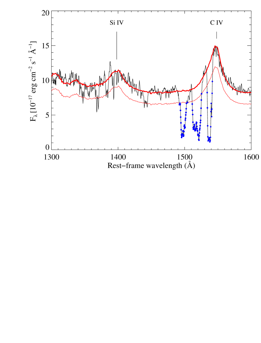
Figure 1: Spectrum of the quasar SDSS J104109.86$+$001051.76 featuring broad absorption lines. The fit to the quasar continuum is shown by the thick line. The thin line represents a decrement of 20% in the quasar flux. Pixels satisfying the BAL criteria inside the running windows (see text) are marked with blue dots.

We excluded the quasars whenever ${\cal R}(\lambda)$ is continuously less than 0.8 over 1000 ${\rm km\,s^{-1}}$, or ${\cal R}(\lambda)<0.8$ over at least 75% of a 3000 ${\rm km\,s^{-1}}$ wide window, running between 1350 and 1550 Å in the quasar’s rest frame. With this definition, we are most sensitive to broad absorption lines with balnicity indexes (BI) larger than 1000 ${\rm km\,s^{-1}}$. The balnicity index (BI) characterises the strength of a BAL (see e.g. Gibson et al. 2009). Note that the core of a damped Ly-$\alpha$ absorption will be larger than this value, so that possible broad H i, O vi and/or N v lines from systems with BI $<1000$ ${\rm km\,s^{-1}}$ have little chance to mimic a DLA. The procedure excludes 1258 BAL quasars among the 9597 quasars left after the previous steps, i.e. after checking for adequate signal-to-noise ratio and redshift range available along the line of sight.

We have checked this automatic procedure by comparing our list of rejected quasars with the catalogue of SDSS BAL quasars from Trump et al. (2006). Fig. 2 shows the balnicity index distribution of all quasars in Trump et al. (2006) (unfilled histogram) and that of the quasars our procedure excludes (red shaded histogram), the difference is shown as a blue shaded histogram. It can be seen that for BI $>$ 500 km s^-1 our procedure misses very few BAL QSOs. We have checked that the missed BAL QSOs have no strong O vi, H i or N v absorption line that could mimic a DLA.

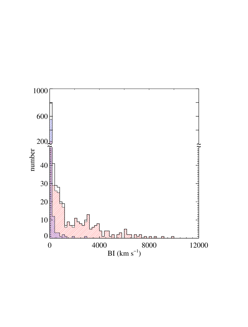
Figure 2: Balnicity index (BI) distribution of the quasars in common with the BAL catalogue of Trump et al. (2006) (solid black line histogram). The BI measurements are from these authors. The red right-dashed histogram corresponds to the quasars identified as BAL by our procedure, while the blue left-dashed histogram represents the distribution of the Trump et al. quasars that are not removed by our procedure. Very few BAL quasars with BI $>$ 500 km s^-1 are missed by our automatic procedure.

We are thus left with the spectra of 8339 QSOs, without strong BALs and with sufficient signal-to-noise ratio to search for damped Lyman-$\alpha$ systems. We call this sample $\mathcal{S}$${}_{QSO}^{0}$. Note that the study of Prochaska & Wolfe (2009, hereafter PW09) using DR5 is based on 7482 QSOs.

3 Detection of DLAs and $N({H\textsc{i}})$ measurements

DLA candidates are generally identified in low-resolution spectra by their large Ly-$\alpha$ equivalent widths ($W_{\rm r}\geq 10$ Å) and are then confirmed by higher spectral resolution observations (e.g. Wolfe et al., 1995). However the resolving power of SDSS spectra ($R=\lambda/{\delta\lambda}\sim 1800$) is high enough to detect the wings of damped Lyman-$\alpha$ lines. Therefore, it is possible not only to identify these lines but also to measure the corresponding H i column densities from Voigt-profile fitting. Note that, because $R$ is constant along the spectrum, the pixel size is constant in velocity-space and DLA profiles of a given $N({H\textsc{i}})$ are equivalently sampled by the same number of pixels, regardless of their redshift.

The number of candidates in the SDSS is so large that the detection techniques must be automatised. Prochaska & Herbert-Fort (2004) searched for DLA candidates in SDSS spectra by running a narrow window along the spectra to identify the core of the DLA trough as a region where the signal-to-noise ratio is significantly lower than the characteristic SNR in the vicinity. Candidates were then checked by eye and the H i column density measured by Voigt-profile fitting interactively.

We develop here a novel approach which makes use of all the information available in the DLA profile and, most importantly, is fully automatic.

3.1 Search for strong absorptions

The technique is based on a Spearman correlation analysis. At each pixel $i$ in the spectrum, corresponding to a given redshift for Lyman-$\alpha$, synthetic Voigt profiles corresponding to different column densities ($N({H\textsc{i}})_{\rm j}$) differing by 0.1 dex are successively correlated with the observed spectrum over a velocity interval [${\rm v}_{\rm min}$,${\rm v}_{\rm max}$] corresponding to a decrement larger than 20% in the Voigt profile. Each redshift ($z_{\rm i}$) for which the Spearman’s correlation coefficient is larger than 0.5 with high significance ($>5\sigma$) is recorded. We then add the criterion that the area between the observed ($F_{\rm obs}$) and synthetic ($F_{\rm synt}$) profiles is less than the integrated error array ($E_{\rm obs}$) on the interval [$v_{\rm min}$,$v_{\rm max}$]:

$$\int_{{\rm v}_{\rm min}}^{{\rm v}_{\rm max}}(F_{\rm obs}-F_{\rm synt})^{+}\leq\int_{{\rm v}_{\rm min}}^{{\rm v}_{\rm max}}E_{\rm obs},$$ (1)

where $(F_{\rm obs}-F_{\rm synt})^{+}=(F_{\rm obs}-F_{\rm synt})$ if $(F_{\rm obs}>F_{\rm synt})$ and 0 otherwise. This definition allows the DLA line to be blended with intervening Lyman-$\alpha$ absorbers.

The ($z_{\rm i},N({H\textsc{i}})_{\rm j}$) pair with highest correlation for each DLA candidate is then recorded. This provides a list of DLA candidates with first guesses of $N({H\textsc{i}})$ and $z_{\rm abs}$.

3.2 Fits of Lyman-$\alpha$ and metal lines

For each candidate, we perform, in the vicinity of the candidate redshift $z_{\rm i}$, a cross-correlation of the observed spectrum with an absorption template representing the most prominent low-ionisation metal absorption lines (C ii$\lambda 1334$, Si ii$\lambda$1526, Al ii$\lambda 1670$, Fe ii$\lambda 1608,2344,2374,2382,2586,2600$, Mg ii$\lambda\lambda 2796,2803$). The template is a variant of a binary mask (similar to those used to derive stellar radial velocities, see e.g. Baranne et al., 1996), where each absorption line is represented by a Gaussian with a width matching the SDSS spectral resolution (see top panel of Fig. 3). We restrict the mask to the metal lines expected in the red of the QSO Ly-$\alpha$ emission line to avoid contamination by Ly-$\alpha$ forest lines. We then obtain a sharp cross-correlation function (CCF, Fig. 3) which is itself fitted with a Gaussian profile to derive a measurement of the redshift with an accuracy better than $10^{-3}$. Voigt profiles are fitted to each metal line after determination of the local continuum, providing a measure of their equivalent widths. In case of non-detection of low-ionisation lines, the same procedure is repeated to detect C iv and Si iv absorption lines. Finally, when no metal absorption line is detected automatically, we keep the redshift obtained from the best correlation with the synthetic Ly-$\alpha$ profile ($z_{\rm j}$, see Section 3.1).

A Voigt-profile fit of the damped Lyman-$\alpha$ absorption is then performed to derive an accurate measurement of $N({H\textsc{i}})$ (bottom-right panel of Fig. 3), taking as initial value the guess on $N({H\textsc{i}})$ from the best synthetic profile correlation and fixing the redshift to the value derived as described above. Absorption lines from the Ly-$\alpha$ forest are ignored iteratively by rejecting deviant pixels with a smaller tolerance at each iteration.

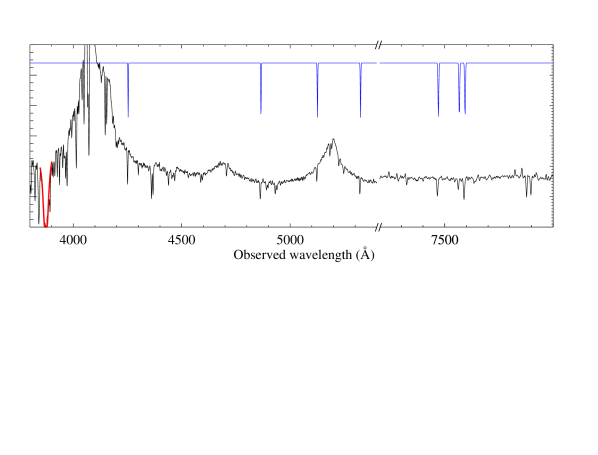
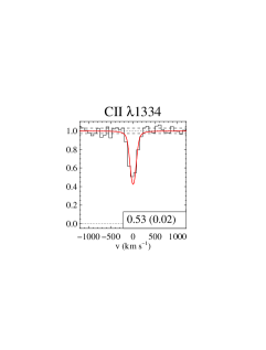
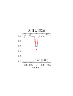
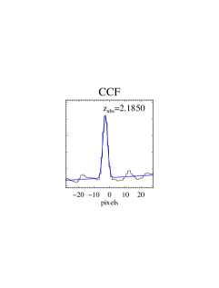
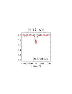
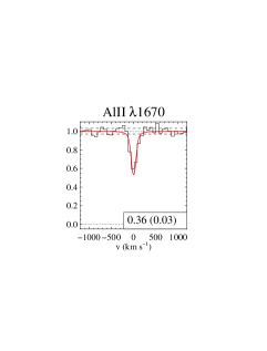
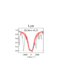
Figure 3: Example of the SDSS spectrum of J 152529.18$+$292813.18 with a DLA line at $\lambda_{\rm obs}\sim 3880\leavevmode\nobreak\ {\AA}$ (top panel). The mask (template of low-ionisation absorption lines) used to derive an accurate redshift ($z_{\rm abs}$ = 2.1850) from the cross-correlation function (shown in panel CCF with the origin of the pixel scale set from the first guess) is overplotted in blue in the upper panel. The automatic fits to a few metal absorption lines are shown in the left-hand side and middle panels (C ii $\lambda 1334$, Si ii $\lambda 1526$, Fe ii $\lambda 1608$, Al ii $\lambda 1670$). Rest-frame equivalent widths and associated errors are indicated (in Å) at the bottom of each panel. The automatic Voigt-profile fit to the damped Ly-$\alpha$ line is overplotted to the observed spectrum in the bottom-right panel. The shaded area corresponds to the uncertainty on the column density ($N({H\textsc{i}})=10^{20.56\pm 0.21}$ ${\rm cm}^{-2}$).

For each system, we obtain an accurate measurement of the absorber’s redshift, the H i column density and the equivalent width of associated metal absorption lines, without any human intervention. We found 1426 absorbers with $\log N({H\textsc{i}})\geq 20$, among which 937 have $\log N({H\textsc{i}})\geq 20.3$. This is the largest DLA sample ever built. The distributions of H i column densities and redshifts for the whole sample is shown on Fig. 4.

Figure 4: Top: Histogram of H i column densities for the 1426 absorbers automatically detected in SDSS DR7. The vertical dotted line marks the traditional DLA threshold value of $\log N({H\textsc{i}})=20.3$. Bottom: Histogram of absorption redshifts for the same sample.

3.3 Accuracy of the measurements and systematic errors

Direct comparisons can be performed between the sample of PW09, derived from SDSS Data Release 5, and the corresponding sample from our survey. Indeed, one would like to assess the completeness of each sample and the reliability of the corresponding detection procedures.

For this, we consider only systems that are detected along lines of sight covered by both surveys. We compare the lists of systems with $\log N({H\textsc{i}})>21$ from this work and from PW09. We check whether $\log N({H\textsc{i}})>21$ systems from a given survey are detected in the other survey, whatever the column density estimated in the second survey is. The limit on $N({H\textsc{i}})$ is chosen high enough so that no system is excluded because of errors. In addition, these systems are the most important for the analysis because, as we will show, they contribute to more than one half of $\Omega_{\rm g}^{\rm DLA}$. Only one such DLA (at $z_{\rm abs}=3.755$ towards J130259.60$+$433504.5) among 76 in the PW09 list has been missed by our procedure, due to spurious lines leading to a wrong CCF redshift measurement. This means that our completeness at $\log N({H\textsc{i}})>21$ is about $99\%$. In turn, we discovered 6 $\log N({H\textsc{i}})>21$ DLAs, with redshifts in the range $z=2.3-3.8$, that are not in the PW09 list when they should be since the corresponding lines of sight have been considered and the redshift of the DLA covered. These are J100325.13$+$325307.0 ($z_{\rm abs}$=2.330); J205509.49$-$071748.6 ($z_{\rm abs}$=3.553); J093251.00$+$090733.9 ($z_{\rm abs}$=2.342), J133042.52$-$011927.5 ($z_{\rm abs}$=2.881); J092914.49$+$282529.1 ($z_{\rm abs}$=2.314) and J151037.18$+$340220.6 ($z_{\rm abs}$=2.323). Associated metal lines are detected for five of them.

The completeness at smaller $N({H\textsc{i}})$ is more difficult to estimate because of the uncertainty of individual measurements. We compared however our detections to that of PW09 and found that we recover more than 96% of their systems with most of the DLAs missed having $\log N({H\textsc{i}})\sim 20.3$. We also checked visually one hundred randomly-selected DLAs and found that about 3% of the systems in our sample are false-positive detections (1% at $z<3.2$ and 7% at $z>3.2$). The completeness of both samples (PW09 and ours) is sufficiently high to have little influence on the determination of the cosmological mass density of neutral gas.

Next, we compare the $N({H\textsc{i}}$) measurements for the same systems in the two samples. Fig. 5 shows the distribution of the difference in the DLA column densities, $\Delta\log N({H\textsc{i}})=\log N({H\textsc{i}})_{\rm this\leavevmode\nobreak\ work}-\log N({H\textsc{i}})_{\rm PW09}$, for the whole sample (black), $z<3$ (blue), $3<z<3.5$ (orange) and $z>3.5$ (red). These distributions are corrected from the truncating effect at $\log N({H\textsc{i}})=20.3$, i.e. from the fact that some systems may have $\log N({H\textsc{i}})\geq 20.3$ in one sample but $\log N({H\textsc{i}})<20.3$ in the other sample. Only systems for which the opposite of $\Delta\log N({H\textsc{i}})$ is also allowed are considered. The uncorrected distribution for the whole sample is shown as a dotted line.

The dispersion in the whole sample is about 0.20 dex and matches the typical error on individual $N({H\textsc{i}})$ measurements. There is a small systematic difference that increases with redshift from less than 0.03 dex at $z<3$ to 0.05 dex at $z>3.5$, which is likely due to the increasingly crowded Ly-$\alpha$ forest at higher redshift.

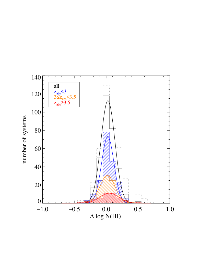
Figure 5: Distribution of the difference in the column density measurements from the two surveys, $\Delta\log N({H\textsc{i}})=\log N({H\textsc{i}})_{\rm this\leavevmode\nobreak\ work}-\log N({H\textsc{i}})_{\rm PW09}$, for the whole sample (black), $z<3$ (blue), $3<z<3.5$ (orange) and $z>3.5$ (red). Distributions are corrected from the $\log N({H\textsc{i}})=20.3$ truncating effect (see text). The non-corrected distribution for the whole sample is represented by the dotted histogram.

4 Results

In this section, we present the statistical results from our DLA survey. Here, we use the standard definitions for the different statistical quantities.

The absorption distance $X$ is defined as

$$X(z)=\int_{0}^{z}(1+z^{\prime})^{2}{{\mbox{$H_{0}$}}\over{H(z^{\prime})}}dz^{\prime},$$ (2)

where $H_{0}$ is the Hubble constant and $H(z)=\mbox{$H_{0}$}\left[{(1+z^{3})\Omega_{\rm m}-(1+z)^{2}(\Omega_{\rm m}+\Omega_{\Lambda}-1)+\Omega_{\Lambda}}\right]^{1/2}$. The cosmological mass density of neutral gas, $\Omega_{\rm g}^{{H\textsc{i}}}$, is given by

$$\Omega_{\rm g}^{{H\textsc{i}}}(X)dX\equiv{{\mu m_{\rm H}\mbox{$H_{0}$}}\over{c\rho_{\rm c}}}\int_{N_{\rm min}}^{N_{\rm max}}N({H\textsc{i}})f_{{H\textsc{i}}}(N,X)dX,$$ (3)

where $f_{{H\textsc{i}}}(N,X)$ is the $N({H\textsc{i}})$ frequency distribution (i.e. $f_{{H\textsc{i}}}(N,X)dNdX$ is the number of systems within $(N,N+dN)$ and $(X,X+dX)$), $\mu=1.3$ is the mean molecular mass of the gas and $\rho_{\rm c}$ is the critical mass density. Setting $N_{\rm min}=2\times 10^{20}$ ${\rm cm}^{-2}$  and $N_{\rm max}=\infty$ gives $\Omega_{\rm g}^{\rm DLA}$, the cosmological mass density of neutral gas in DLAs. Since at the column densities of DLAs the gas is neutral, this is also the total mass density of the gas in DLAs. In the discrete limit, $\Omega_{\rm g}^{\rm DLA}$ is given by:

$$\Omega_{\rm g}^{\rm DLA}={{\mu m_{\rm H}\mbox{$H_{0}$}}\over{c\rho_{c}}}{{\Sigma N({H\textsc{i}})}\over{\Delta X}},$$ (4)

where the sum is calculated for systems with $\log N({H\textsc{i}})\geq 20.3$ along lines of sight with a total pathlength $\Delta X$. We adopt a $\Lambda$CDM cosmology with $\Omega_{\Lambda}=0.7$, $\Omega_{\rm m}=0.3$, and $\mbox{$H_{0}$}=70$ ${\rm km\,s^{-1}}$ Mpc^-1 (e.g. Spergel et al., 2003).

4.1 Sensitivity function

We present in Fig. 6 the sensitivity functions $g(z)$, i.e. the number of lines of sight covering a given redshift, for the different DLA surveys discussed in this paper.

The redshift sensitivity of SDSS is significantly larger than that of the largest QSO compilation prior to SDSS (Péroux et al., 2003) at any redshift larger than 2.2. The higher sensitivity ($\sim 30\%$) of our SDSS sample compared to that of PW09 over the redshift range $z\sim 2.2-3.5$ reflects the increase in the number of observed quasars between the two data releases (DR5 and DR7). At $z>3.5$, the sensitivity of the PW09 quasar sample is higher than that presented here. This is due to (i) the choice by these authors to exclude only 3000 km s^-1 from the emission redshift of the quasar whereas we exclude 5000 km s^-1 to avoid the proximity effect, (ii) the slightly strongest constraint on SNR we impose when including quasar spectra in our survey, (iii) the inclusion of quasars with some BAL activity in the PW09 sample and (iv) the fact that we restrict our quasar sample to those with confidence on the redshift measurement higher than 0.9. Very few quasars are detected in SDSS at $z>4$ and the determination of $\Omega_{\rm g}^{\rm DLA}$ at these redshifts would benefit of dedicated surveys (see Guimarães et al., 2009). We note that among the ten $z_{\rm em}\geq 5$ quasars in the PW09 sample, J 165902.12$+$270935.1 was spectroscopically mis-classified as ‘galaxy’ instead of ‘QSO’ by the SDSS while the redshift confidence for J 075618.13$+$410408.5 is smaller than 0.9. These lines of sight were therefore not included in our quasar sample (see Sect. 2). Furthermore, five of these quasars have been rejected from our statistical sample, either because of BAL activity (Sect. 2.3) or because of a low mean signal-to-noise ratio of the spectrum (Sect. 2.2).

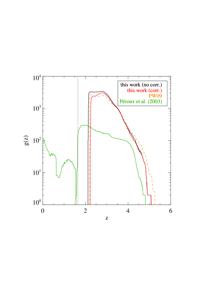
Figure 6: Redshift sensitivity function $g(z)$ of the different DLA surveys considered in this paper. The black and red curves represent respectively the sensitivity of our survey without ($\delta{\rm v}=0$ ${\rm km\,s^{-1}}$) and with ($\delta{\rm v}=10\,000$ ${\rm km\,s^{-1}}$) correction of the edge-effect bias (see Sect. 4.2). The green curve is from the sample built by Péroux et al. (2003) whereas the orange dashed curve represents the DR5 sensitivity from Prochaska & Wolfe (2009). The vertical dotted line corresponds to $z=1.65$, which is the redshift below which the Ly-$\alpha$ line cannot be observed from the ground because of the atmospheric absorption.

4.2 Importance of systematic effects

With the large number of quasar spectra available in SDSS, we reach a level at which systematic effects become more important than statistical errors. In particular, the statistical results of the survey are very sensitive to the determination of the total absorption distance $\Delta X$.

The presence of a DLA absorption line significantly attenuates the quasar flux and decreases the signal-to-noise ratio of the spectrum. Therefore, if a DLA line is present at the blue end of the spectrum, the minimum redshift considered along the line of sight prior to any search for DLA absorption can be overestimated. The corresponding redshift range is rejected a priori because of the presence of the DLA. The immediate consequence is that the presence of a strong absorption can preclude its inclusion in the statistical sample (see Fig. 7). We expect this effect to be important for large $N({H\textsc{i}})$, when $\lambda_{\rm DLA}$ is close to the blue-end of the spectrum (at 3800 Å), and when the signal-to-noise ratio of the spectrum is low. Note that the bias we describe here can affect all DLA surveys.

In order to assess the severity of this effect, we artificially added damped Ly-$\alpha$ absorptions to the spectra of quasars from sample $\mathcal{S}$${}_{QSO}^{0}$. Column densities are in the range $\log N({H\textsc{i}})=20.3-22$ and redshifts in the range $2.2\leq z\leq 2.4$. We applied our automatic procedure to define $z_{\rm min}$ and compare the minimum redshift obtained along each line of sight with ($z_{\rm min}^{0,DLA}$) and without ($z_{\rm min}^{0}$) the DLA. For each set of values ($z_{\rm abs}$, $\log N({H\textsc{i}})$), we calculated the fraction of DLAs that are missed because of their influence on the redshift path ($z_{\rm min}^{0,DLA}>z_{\rm abs}$ while $z_{\rm min}^{0}<z_{\rm abs}$). This fraction indicates the severity of the bias. The result of this exercise is shown on Fig. 8. It is clear from this figure that there is indeed a severe bias against the presence of DLAs at the blue end of the spectra. This bias increases, as expected, with decreasing redshift and increasing column density.

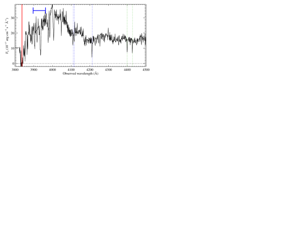
Figure 7: Example of the effect of the presence of a DLA on the determination of $z_{\rm min}$. Because of the DLA absorption near the blue end of the spectrum (thick vertical line), the minimum redshift along this line of sight is set by the automatic procedure redwards of the absorption (and the redshift range considered is marked by an horizontal segment). If the DLA had no effect on the determination of the minimum accessible redshift, then the latter would have been set to the blue end of the spectrum. The consequence is that the DLA is missed, while it should have been included in the sample (see Sect. 4.2). Note that the reality of the DLA is confirmed by the detection of metal lines whose positions are indicated by vertical dotted lines. The spectrum shown in this figure is that of J162131.46$+$234550.8. We propose a procedure to avoid this systematic effect (see Text).

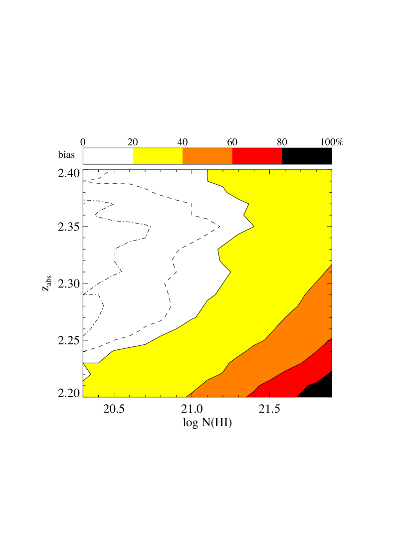
Figure 8: Result of a simulation to estimate the severity of the bias (defined as the percentage of DLAs missed; see Text) due to the incorrect pathlength determination resulting from the presence of a DLA at the blue end of the spectrum as a function of the redshift and neutral hydrogen column density of the absorber. The colour scale is given at the top of the figure. Additionally, the dotted, dashed-dotted and dashed lines represent the 5, 10 and 15% contours, respectively.

We propose to circumvent this problem by adding a systematic velocity shift $\delta v$ to $z_{\rm min}^{0}$ defining $z_{\rm min}$ as:

$$z_{\rm min}=z_{\rm min}^{0}+{{\delta{\rm v}}\over{c}}(1+z_{\rm min}^{0}).$$ (5)

We therefore a priori exclude part of the spectrum at the blue end. This decreases the total pathlength of the survey but guarantees, for a sufficiently large $\delta v$, that any pathlength that would be excluded in the case of the presence of a DLA is a priori excluded from the statistics. In other words, the definition of $[z_{\rm min}-z_{\rm max}]$ will not depend upon the presence of a DLA in this redshift range and the bias will be avoided a priori.

Note that in their survey, Prochaska et al. (2005) are aware of this effect and apply a shift of $\delta{\rm v}=1\,500$ ${\rm km\,s^{-1}}$ which they claim is sufficient to avoid the bias considered as minor. They also restrict their analysis to $z>2.2$ so that the very blue end of the spectrum is not considered. However the wings of a DLA can significantly lower the signal-to-noise ratio over a velocity range as large as several thousands kilometres per second. For example, a $\log N({H\textsc{i}})\sim 21$ DLA lowers the SNR by more than 10% (and obviously up to 100% in the core of the profile) over a velocity range of about 10 000 ${\rm km\,s^{-1}}$. We therefore expect the bias to be corrected only for large values of $\delta{\rm v}$.

We performed the same test as described above with $\delta{\rm v}=2\,500,5\,000,7\,500$ and $10\,000$ ${\rm km\,s^{-1}}$. The different panels of Fig. 9 give the results. It is clear that the bias is still quite strong for $\delta{\rm v}=2\,500$ ${\rm km\,s^{-1}}$ and almost vanishes for $\delta{\rm v}=10\,000$ ${\rm km\,s^{-1}}$.

We will see in the following that the systems with $\log N({H\textsc{i}})\sim 21.3$ contribute most to the total cosmological mass density of neutral gas. The residual bias must therefore be well below 10% for this kind of column densities. This is the case with $\delta{\rm v}=10\,000$ ${\rm km\,s^{-1}}$: only systems with very large column densities ($\log N({H\textsc{i}})>21.9$) and redshifts below 2.3 have $>$ 20% probability to be missed. As we expect about one such system in the whole SDSS survey and at any redshift, the remaining bias is well below the Poissonian statistical error. Applying a $\delta{\rm v}$ shift larger than $10\,000\leavevmode\nobreak\ {\rm km\,s^{-1}}$ would therefore be useless and would unnecessarily decrease the total pathlength of the survey (see Fig. 6).

In order to verify that the bias indeed affects the results from PW09, we searched their quasar sample for DLAs at $z=2.2-2.4$ that their procedure missed. To flag these systems, we could have searched for strong Mg ii absorption lines that have been shown to be good tracers of DLAs (e.g. Rao & Turnshek, 2000), but the corresponding absorption lines are unfortunately redshifted either beyond the SDSS spectrum ($z>2.28$) or at its very red end, where the quality of the spectra becomes very poor. We therefore automatically searched for strong Fe ii absorption lines instead. Out of 57 systems detected this way, 32 are in Prochaska & Wolfe’s statistical sample and 25 have been missed because the minimum redshift is set redwards of the DLA due to the decreased signal-to-noise ratio. Few examples of such DLAs are given in Fig. 10.

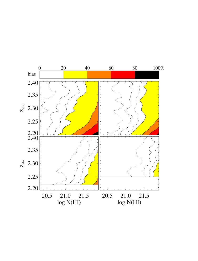
Figure 9: Same as Fig. 8 when applying different corrections. From left to right and top to bottom: $\delta{\rm v}=2\,500,5\,000,7\,500$ and $10\,000\leavevmode\nobreak\ {\rm km\,s^{-1}}$. Colours and line styles are as per Fig. 8.

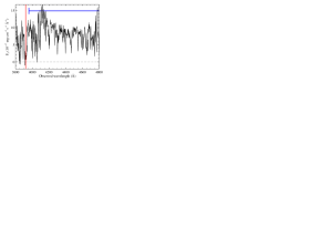
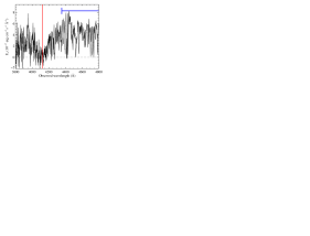
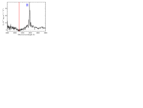
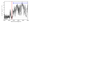
Figure 10: Spectra of four DLAs with $z_{\rm abs}<z_{\rm min}$ in the sample of PW09. The vertical lines show the positions of the Ly-$\alpha$ absorptions and the horizontal segment corresponds to the redshift pathlength (as defined by these authors) probed along each line of sight. In all cases, the presence of metal lines confirm the DLA. From left to right and top to bottom: J092322.86$+$033821.5, J155556.90$+$480015.0, J084006.65$+$362531.6 and J095604.44$+$344415.5.

In the following, we will apply the $\delta v$ cut to avoid the bias (850 bona-fide DLAs are then left in the statistical sample) and correct our statistical results for the reliability of our DLA sample ($\sim 93\%$ at $z>3.2$). Note that, while the first correction will have important consequences, the second correction only has a minor effect on the $\Omega_{\rm g}^{\rm DLA}(z)$ results.

4.3 Frequency distribution

In Fig. 11, we present the $N({H\textsc{i}})$ frequency distribution function $f_{{H\textsc{i}}}(N,X)$ of the whole sample. Vertical error bars are representative of Poissonian statistical errors while horizontal bars represent the $\log N({H\textsc{i}})$-binning (by steps of 0.1 dex). We find that a double power-law (e.g. PW09, ),

$$f_{{H\textsc{i}}}(N,X)=\left\{\begin{array}[]{ll}k_{\rm d}\left({N\over N_{\rm d}}\right)^{\alpha_{\rm d1}}&\mbox{for }N<N_{\rm d}\\ &\\ k_{\rm d}\left({N\over N_{\rm d}}\right)^{\alpha_{\rm d2}}&\mbox{for }N\geq N_{\rm d}\\ \end{array}\right.$$ (6)

or a $\Gamma$-function (e.g. Fall & Pei, 1993; Péroux et al., 2003),

$$f_{{H\textsc{i}}}(N,X)=k_{g}\left({N\over N_{g}}\right)^{\alpha_{g}}e^{(-N/N_{g})}$$ (7)

fit the data equally well ($\chi^{2}_{\nu}=1.1$ and 0.7, respectively). The best fit values of the parameters are summarised in Table 1. Slight differences between the $\Gamma$-function and double power-law fits (see also next Section) are not statistically significant.

Table 1: Parameters of the fits to the $N({H\textsc{i}})$ frequency distribution (see Fig. 11).

Double power law			$\Gamma$ function
$k_{\rm d}$	$=$	$-23.09$	$k_{\rm g}$	$=$	$-22.75$
$N_{\rm d}$	$=$	$21.27$	$N_{\rm g}$	$=$	$21.26$
$\alpha_{\rm d1}$	$=$	$-1.60$	$\alpha_{\rm g}$	$=$	$-1.27$
$\alpha_{\rm d2}$	$=$	$-3.48$

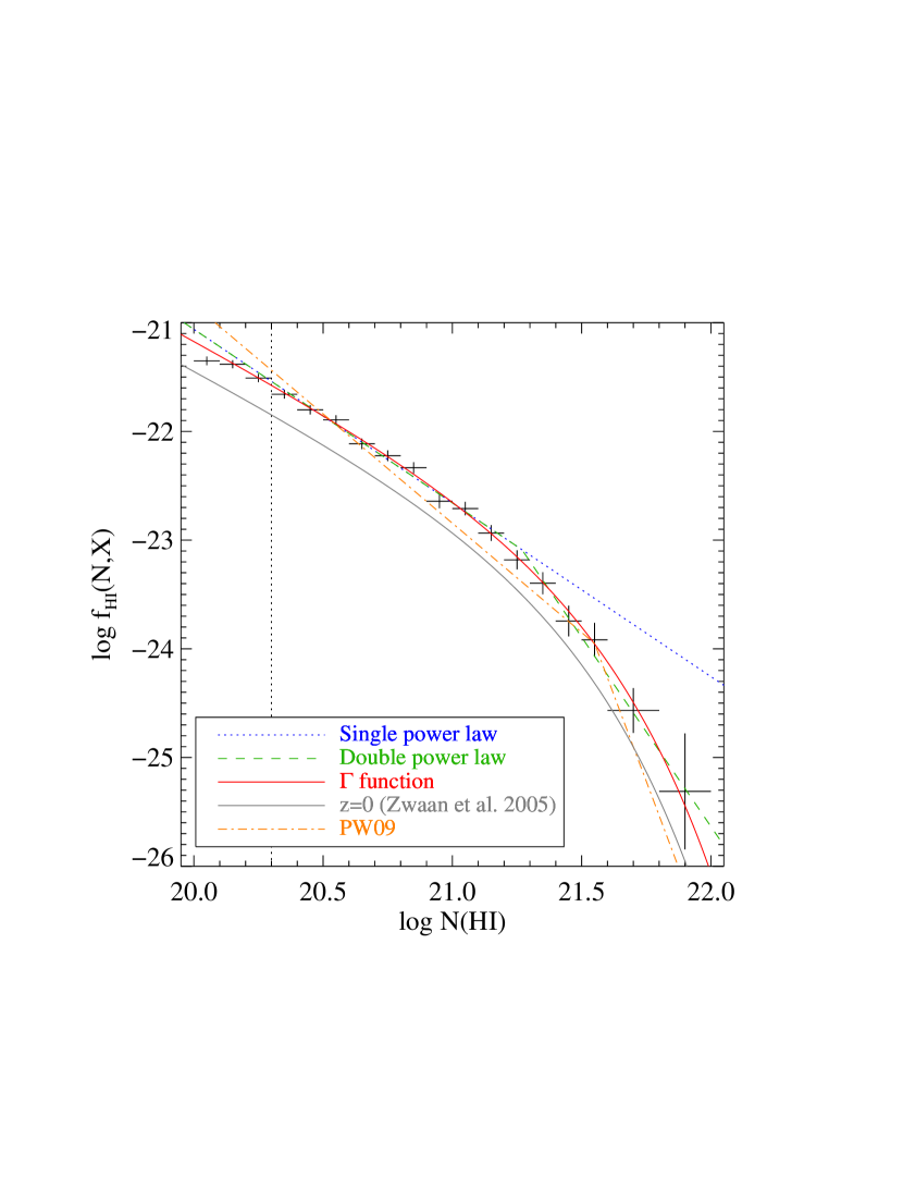
Figure 11: $N({H\textsc{i}})$ frequency distribution of damped Lyman-$\alpha$ systems in SDSS-DR7 from our automatic procedure. Fits to the observations by a single power law, a double power law and a gamma function are given as, respectively, a dotted blue, dashed green and solid red line. The double-power law fit to the PW09 sample is indicated by the dashed orange line. The $\Gamma$-function fit to the frequency distribution obtained by Zwaan et al. (2005b) from 21-cm observations at $z=0$ is also indicated as a solid grey line for direct comparison.

The slope of the distribution is found to be $\alpha\sim-1.6$ for $N({H\textsc{i}})<21.4$, which is close to what is expected from models of photo-ionised gas in hydrostatic equilibrium (e.g. Petitjean et al., 1992). This is flatter than what is found by Prochaska et al. (2005), $\alpha\sim-2$ for their whole sample (see also PW09, ). Péroux et al. (2005) already mentioned that the slope of the frequency distribution at $N({H\textsc{i}})$ around the conventional DLA threshold is flatter than $-2$.

The slope of $f_{{H\textsc{i}}}(N,X)$ at large $N({H\textsc{i}})$, $\alpha\approx-3.5$, implies that systems with very large column density are very rare. We find a slope much flatter than PW09 ($\alpha\approx-6$). This is probably due to our definite detection of the first DLA with $\log N({H\textsc{i}})=22$, at $z_{\rm abs}=3.286$ towards SDSS J081634$+$144612. We obtained high spectral resolution data for this quasar with UVES in April 2008. The column density, measured from the UVES spectrum, is $\log N({H\textsc{i}})=22.0\pm 0.1$ (see Fig. 12) while the column density derived automatically from the SDSS spectrum is $\log N({H\textsc{i}})=21.92\pm 0.19$. This is the absorber with the largest column density observed to date along a quasar line of sight. Such a column density is similar to that of DLAs detected at the redshift of Gamma-Ray Bursts (e.g. Vreeswijk et al., 2004; Jakobsson et al., 2006; Ledoux et al., 2009). Detailed analysis of this system will be presented in a future paper. Note that from the fit of the frequency distribution, no more than one system like this one is expected in the whole SDSS survey.

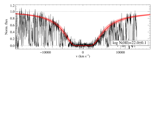
Figure 12: Damped Lyman-$\alpha$ absorption line at $z_{\rm abs}=3.286$ towards SDSS J081634.40$+$144612.86. The neutral hydrogen column density, measured from the Voigt profile fit to the smoothed (7 pixel boxcar) UVES spectrum, is $\log N({H\textsc{i}})=22.0\pm 0.1$. This is the highest H i column density ever measured along QSO lines of sight.

The shape of the $N({H\textsc{i}})$ frequency distribution at high column densities suggests that there is no abrupt transition between neutral hydrogen and molecular hydrogen in diffuse clouds as advocated by (Schaye, 2001). This is supported by the results of Zwaan & Prochaska (2006) who used CO emission maps to show that the H₂ distribution function is a continuous extension of $f_{{H\textsc{i}}}(N,X)$ for high column densities. In addition, there is only a small tendency for increasing H₂ molecular fraction with larger ${H\textsc{i}}$ column density (Ledoux et al., 2003; Noterdaeme et al., 2008a).

4.4 Convergence of $\Omega_{\rm g}^{\rm DLA}$ and the contribution of sub-damped Lyman-$\alpha$ systems

One major issue when measuring the cosmological mass density of neutral gas in DLAs is the convergence of $\Omega_{\rm g}^{\rm DLA}$ at large $\log N({H\textsc{i}})$ values. An artificial cut at large $N({H\textsc{i}})$ was frequently introduced to prevent the integration of a single power-law to diverge. This was justified by small number statistics at the highest column densities. The SDSS allowed PW09 to observe for the first time that the slope of $f_{{H\textsc{i}}}(N,X)$ is steeper than $-2$ for $\log N({H\textsc{i}})>21.5$, directly demonstrating that $\Omega_{\rm g}^{\rm DLA}$ converges.

Figure 13 presents the cumulative cosmological mass density of neutral gas in DLAs as a function of the maximum H i column density from data in our study and from the different fits to the frequency distribution. It is apparent that $\Omega_{\rm g}^{\rm DLA}$ converges by $\log N({H\textsc{i}})=22$.

A change of inflexion in the frequency distribution is apparent at $\log N({H\textsc{i}})\sim 21$. This is best seen on Fig. 14 which gives the slope of the above quantity as a function of $\log N({H\textsc{i}})$. In other words, the area below the curve represents the contribution of the different intervals of $N({H\textsc{i}})$ to the total H i mass density. It is apparent that systems with very large (resp. low) column densities contribute little to the census of neutral gas because of their paucity (resp. low column density). The most important contribution comes from DLAs with $\log N({H\textsc{i}})\sim 21.2$. A simple extrapolation of the $\Gamma$-function fit to column densities smaller than $\log N({H\textsc{i}})=20.3$ shows that sub-DLAs, with $19\la\log N({H\textsc{i}})<20.3$, contribute about 20% of the mass density of neutral hydrogen at $z\ga 2.2$. Extrapolating the double power-law fit gives a sub-DLA contribution to $\Omega^{{H\textsc{i}}}_{\rm g}$ of about 30%.

Although both the power law and the Gamma function are good fits to $f_{{H\textsc{i}}}(N,X)$, it can be seen on Figs. 11 and 14 that the slope of $f_{{H\textsc{i}}}(N,X)$ could be smaller at the low end ($\log N({H\textsc{i}})\sim 20.3$) (Péroux et al., 2005; Guimarães et al., 2009). The gamma function could best reproduce this regime. Furthermore, the double power-law produces a spike seen at $\log N({H\textsc{i}})=21.3$, that is not present in the data. This is due to the arbitrary and somewhat unphysical discontinuous change in the slope of the double power-law fit.

It is interesting to note here that the contribution of the different column densities to $\Omega^{{H\textsc{i}}}_{\rm g}$ at high redshift is very similar to what is observed in the local Universe (Zwaan et al., 2005b). This indicates that the H i surface density profile of the neutral phase at high-$z$ is not significantly different from that observed at $z=0$.

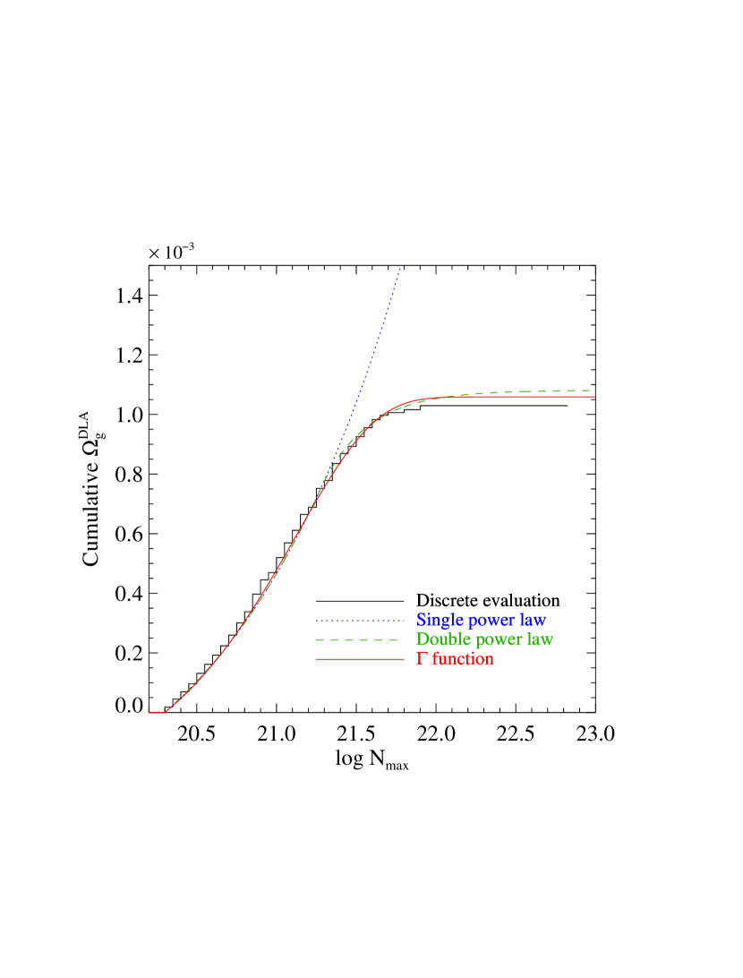
Figure 13: Cumulative cosmological mass density of neutral gas in DLAs as a function of maximum column density. The apparent flattening of the curve at $\log N({H\textsc{i}})\sim 21.7$ implies convergence. Double power-law and $\Gamma$ functions are equally possible solutions while a single power-law diverges and is not representative of the data at high column densities.

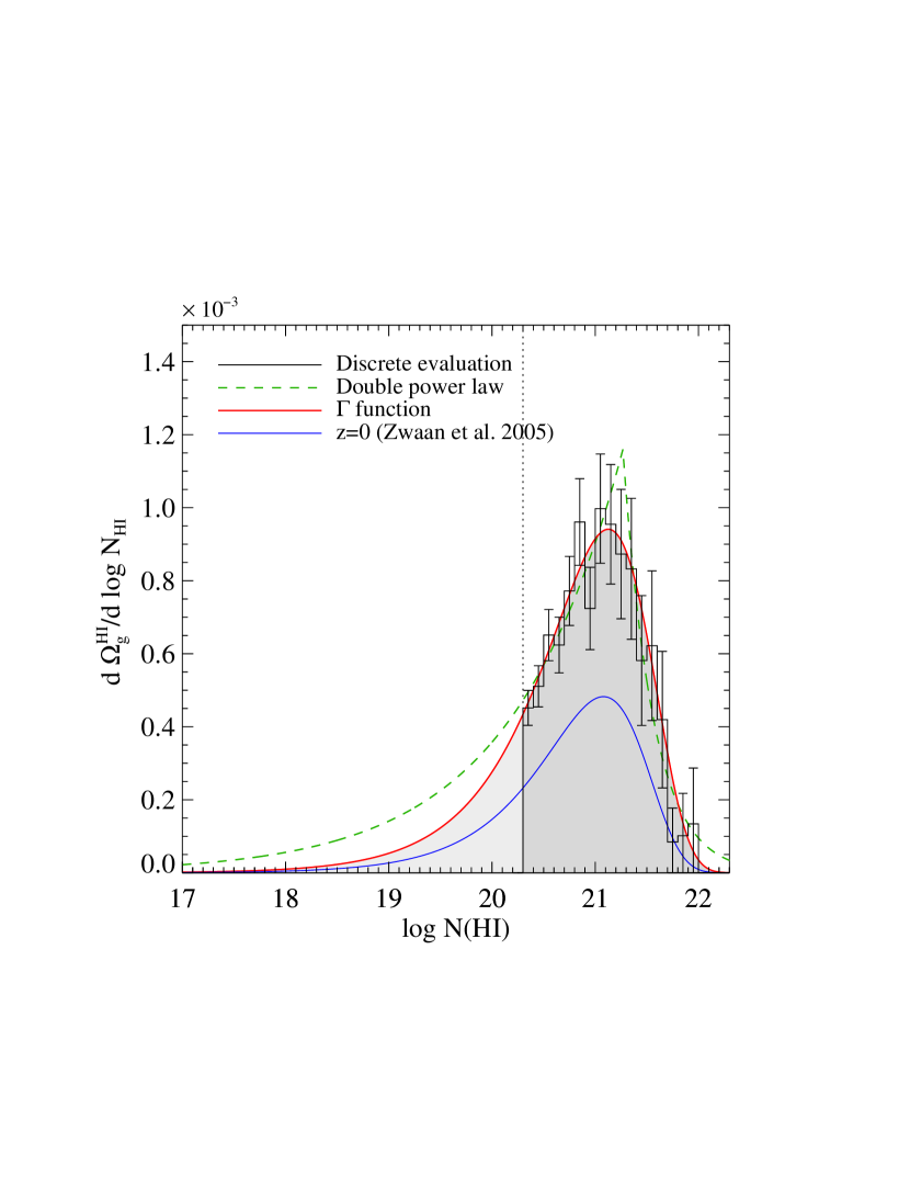
Figure 14: Cosmological mass density of neutral gas contained in systems of different column densities. The dashed-green and red curves correspond respectively to the Double power-law and $\Gamma$-function fits to $f_{{H\textsc{i}}}(N,X)$ in SDSS DR7, while the blue solid curve represents the $\Gamma$-function fit to $f_{{H\textsc{i}}}(N,X)(z=0)$ (Zwaan et al., 2005b).

4.5 Evolution with cosmic time

In this Section, we study the evolution over cosmic time of the cosmological mass density of neutral gas, $\Omega_{\rm g}^{\rm DLA}$. This evolution is the result of several important processes involved in galaxy formation including the consumption of gas during star formation activity but also the consequences of energy releases during the hierarchical building up of systems from smaller blocks (e.g. Ledoux et al., 1998; Haehnelt et al., 1998), or the ejection of gas from the central parts of massive halos into the intergalactic medium through galactic winds (Fall & Pei, 1993).

Storrie-Lombardi & Wolfe (2000) and Péroux et al. (2003) claimed an increase of $\Omega_{\rm g}^{\rm DLA}$ when $z$ decreases from $z\sim 3$ to $z\sim 2$. This is due to the lack in their sample of high column density DLAs at high redshift. From their SDSS DLA search, Prochaska et al. (2005) observe on the contrary a significant decrease of $\Omega_{\rm g}^{\rm DLA}$ between $z\sim 4$ and $z\sim 2$. They interpret this as the result of neutral gas consumption by star formation activity and/or the ejection of gas into the intergalactic medium. The value they derive for $\Omega_{\rm g}^{\rm DLA}$ at $z=2.2$ is almost equal to that at $z=0$, indicating very little or no evolution of the cosmological mass density of neutral gas over the past ten billion years (see PW09, ). We argue here that the differences between these results are artificial and can be reconciled within errors at least up to $z\sim 3.2$.

On the one hand, the redshift pathlength probed along SDSS lines of sight should be restricted so that the edge bias described in Section 8 is avoided. We applied to the PW09 sample the same velocity cut as for our sample and find, as expected, that both samples yield similar results (see Fig. 15). The differences between the measurements from the two SDSS samples are within statistical error bars and are mainly due to slightly higher completeness and larger number statistics of our sample. The immediate implication of the edge-effect correction is that it cannot be claimed that $\Omega_{\rm g}^{\rm DLA}$ does not evolve from $z=2.2$ to $z=0$.

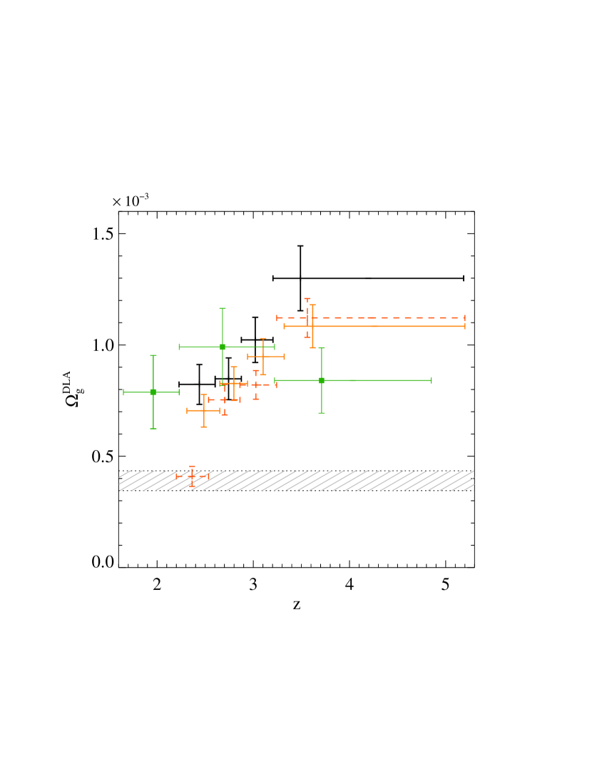
Figure 15: The cosmological mass density of neutral gas in DLAs, $\Omega_{\rm g}^{\rm DLA}$, as a function of redshift for $z>1.65$. Vertical error bars represent the 1 $\sigma$ uncertainties on the measurements while horizontal error bars represent the redshift bins under consideration. Black error bars are our measurements at $z>2.2$. Orange error bars are derived from the PW09 sample when applying a $\delta{\rm v}=10\,000$  ${\rm km\,s^{-1}}$ cutoff to correct for the edge-effect (see Section 4.2 and Eq. 5). The uncorrected values derived from the same sample are shown in dashed orange error bars. The green squares are derived from the sample of Péroux et al. (2003) using a different binning compared to that adopted by these authors. Finally, the hashed region represent the 1 $\sigma$ range on $\Omega_{\rm g}^{\rm DLA}$ at $z=0$ from Zwaan et al. (2005b). We note also that the amount of baryons in stars at $z=0$ is $\Omega_{\star}=(2.5\pm 1.3)\times 10^{-3}$ (Cole et al., 2001).

On the other hand, we also note that a decrease of $\Omega_{\rm g}^{\rm DLA}$ with decreasing redshift cannot be excluded from the sample of Péroux et al. (2003). Indeed, a different binning of their data shows that they are actually consistent with a decrease of $\Omega_{\rm g}^{\rm DLA}$ over the redshift range $z\sim$ 3.2 $-$ 2.2 (see Fig. 15). In addition, while the sample from Péroux et al. is large enough to obtain a reasonable measurement of $\Omega_{\rm g}^{\rm DLA}$ at high redshift, it is probably too small to infer strong conclusions on its evolution. Fig. 16 illustrates the effect of the sample size on the determination of $\Omega_{\rm g}^{\rm DLA}$. We construct randomly selected SDSS QSO sub-samples of increasing total path length, $\Delta X$, and calculate the ratio $\Omega/\Omega_{\rm o}$ of $\Omega_{\rm g}^{\rm DLA}$ values from the subsample and the whole SDSS sample. Note that the survey used in the present paper has $\Delta X$ = 11 099 whereas Prochaska & Wolfe’s survey has $\Delta X$ = 8 475 (applying the new definition of $z_{\rm min}$) and Péroux et al.’s survey has $\Delta X$ = 1 540.

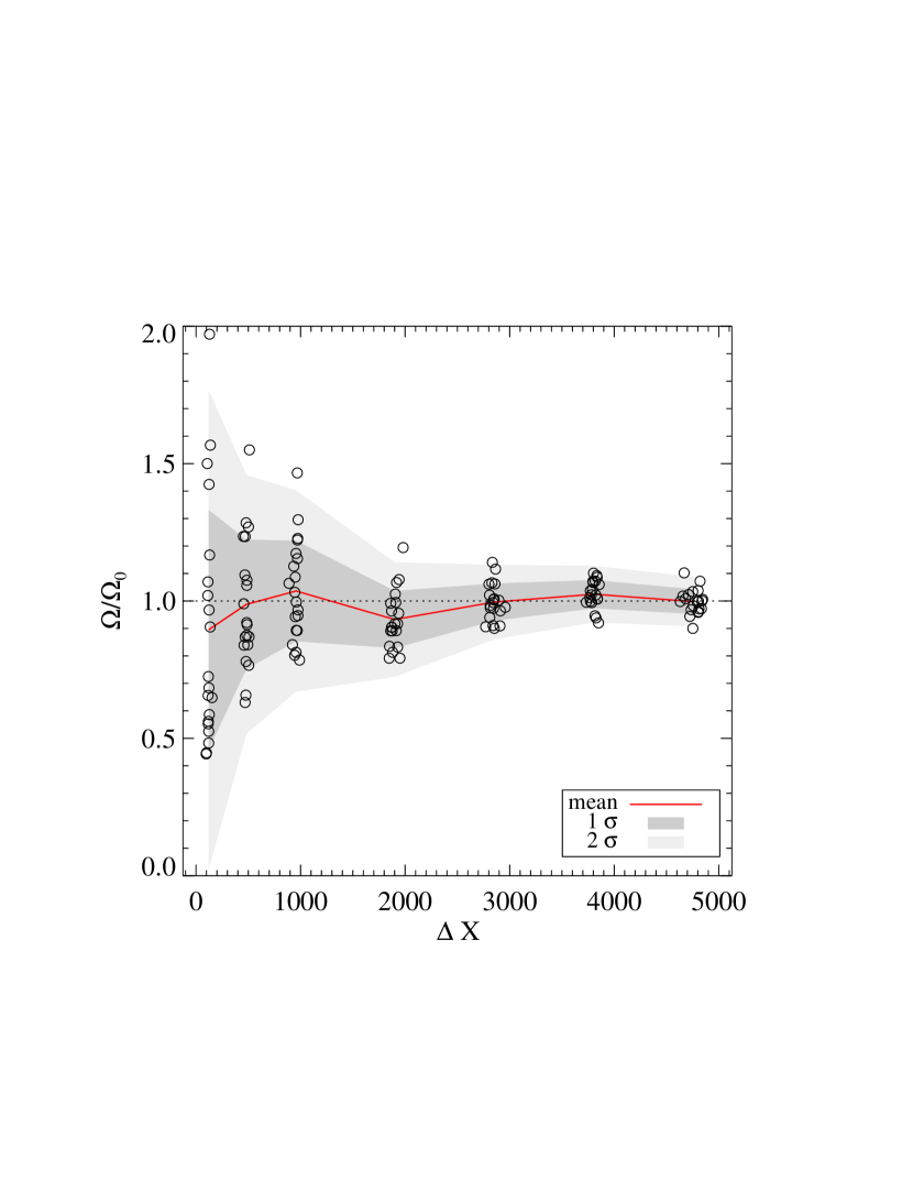
Figure 16: Statistical uncertainty on the determination of $\Omega_{\rm g}^{\rm DLA}$ as a function of the sample size. Each circle represents the ratio between the measurement of $\Omega_{\rm g}^{\rm DLA}$ for a randomly selected sample of total absorption pathlength $\Delta X$ ($\Omega$) and that obtained from the full SDSS sample, $\Omega_{\rm o}$. Note that $\Delta X$ = 1 540, 8 475 and 11 099 in, respectively, Péroux et al. (2003), Prochaska & Wolfe (2009, after correcting for the edge-bias) and the present work.

All this reconciles the SDSS measurements with the results from Péroux et al. (see Fig. 17). It can be seen also that the points at $z\sim 2$ are consistent with those at lower redshift given their large error bars (Rao et al., 2006). Note also that the value we derive at $z\sim 2.4$ is consistent with that obtained from the Hamburg-ESO survey ($\Omega_{\rm g}^{\rm DLA}\sim 1$, A. Smette, private communication; Smette et al., 2005).

At redshifts above $z=3.2$, there is still a discrepancy between the results from SDSS and that from previous surveys (see Fig. 15). As pointed out by Prochaska et al. (2005), the size of the samples prior to SDSS were insufficient to detect the convergence of $\Omega_{\rm g}^{\rm DLA}$ at large $N({H\textsc{i}})$. Therefore, the inclusion of a single large column density system in these samples could change the results on $\Omega_{\rm g}^{\rm DLA}$ significantly. In turn, the low spectral resolution of SDSS combined with a dense Ly-$\alpha$ forest could lead to slightly overestimate the column densities of high-$z$ DLAs.

The measurement of the cosmological mass density of neutral gas at intermediate and low redshifts is a difficult task. The little incidence of DLAs and the need for observations from space have lead to samples of limited sizes. Rao & Turnshek (2000) and Rao et al. (2006) used a novel technique to measure $\Omega_{\rm g}^{\rm DLA}$ at $0.1<z<1.6$. They searched for the Ly-$\alpha$ absorption associated to Mg ii systems, which statistics is very large at those redshifts. The corresponding values of $\Omega_{\rm g}^{\rm DLA}$ are high and therefore have been extensively discussed in the literature. In particular, PW09 concluded that the values obtained at $z\sim 1$ by Rao et al. (2006) are difficult to reconcile with the value they obtained at $z\sim 2.2$ and suffer from a statistical fluke or an observational bias. After correcting for the edge bias we discussed earlier it can be seen that the SDSS results are no more incompatible with the Rao et al. (2006) results. However, it is still possible that the high values of $\Omega_{\rm g}^{\rm DLA}$ from Rao et al. are overestimated due to systematics associated with the selection of low and intermediate redshift DLAs directly from strong Mg ii absorption (see Péroux et al., 2004; Dessauges-Zavadsky et al., 2009). Only a large blind survey for DLAs at $z\sim 1$ could solve this issue.

Note also that $\Omega_{\rm g}^{\rm DLA}(z\sim 2)$, obtained from the sample of Péroux et al. (2003), is almost equal to $\Omega_{\rm g}^{\rm DLA}(z\sim 2.2)$, obtained here from SDSS-DR7. This could indicate a flattening of $\Omega_{\rm g}^{\rm DLA}(z)$ at $z\sim 2$. Large intermediate-redshift optical and radio surveys are therefore still required to constrain the evolution of $\Omega_{\rm g}^{\rm DLA}$ from $z=2$ to $z=0$ (see discussion in Gupta et al., 2009).

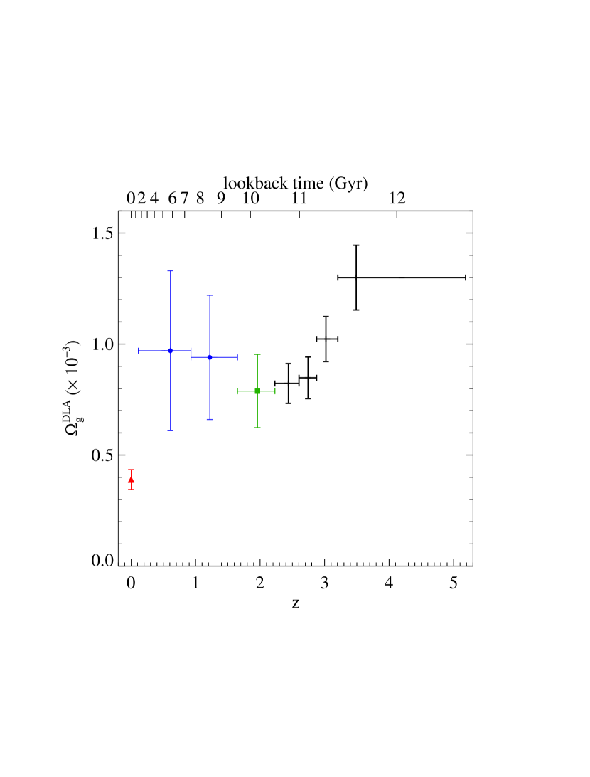
Figure 17: Cosmological mass density of neutral gas in DLAs, $\Omega_{\rm g}^{\rm DLA}$, as a function of redshift. The red triangle at $z=0$ is the value from 21-cm maps by Zwaan et al. (2005b). The blue filled circles at $z\sim 1$ are the measurements of $\Omega_{\rm g}^{\rm DLA}$ from Rao et al. (2006). The green square at $z\sim 2$ is derived from the sample of Péroux et al. (2003). Measurements at $z>2.2$ are from the present work base on SDSS DR7.

Table 2: The cosmological mass density of neutral gas in DLAs from this work (SDSS-DR7)

$z$	$\left<z\right>^{a}$	$\Delta X$	$\Omega_{\rm g}^{\rm DLA}$ ($\times 10^{-3}$)
2.23-2.60	2.44	2774	0.82$\pm$0.09
2.60-2.88	2.74	2774	0.85$\pm$0.09
2.88-3.20	3.02	2774	1.03$\pm$0.10
3.20-5.19	3.49	2774	1.29$\pm$0.15

^a median redshift corresponding to half the total pathlength $\Delta X$ in the redshift bin.

5 Conclusion

We have demonstrated the feasibility and the robustness of a fully automatic search of SDSS-DR7 for DLA systems based on the identification of DLA profiles by correlation analysis. This led to the identification of about one thousand DLAs, representing the largest DLA database to date. We tested the accuracy of the $N({H\textsc{i}})$ measurements and quantified the high level of completeness and reliability of the detections.

In agreement with previous studies (Péroux et al., 2003; Prochaska et al., 2005; Prochaska & Wolfe, 2009), we show that a single power-law is a poor description of the $N({H\textsc{i}})$-frequency distribution at $\log N({H\textsc{i}})\geq 20.3$. A double power-law or a $\Gamma$ function give better fits. The finding of one $\log N({H\textsc{i}})=22$ DLA, confirmed by UVES high spectral resolution observations, shows that the slope of $f_{{H\textsc{i}}}(N,X)$ at $\log N({H\textsc{i}})>21.5$ is $-3.5$.

The convergence of $\Omega_{\rm g}^{\rm DLA}$ for large $N({H\textsc{i}})$ indicates that the cosmological mass density of neutral gas at $z\sim 2.2-5$ is dominated by bona-fide damped Lyman-$\alpha$ systems. The relative contribution of DLAs reaches its maximum around $\log N({H\textsc{i}})=21$, similar to what is observed in the local Universe. The paucity of very high-column density DLAs implies that they contribute for only a small fraction to the cosmological mass density of neutral gas. On the other hand, an extrapolation of $f_{{H\textsc{i}}}(N,X)$ at $\log N({H\textsc{i}})<20.3$ suggests that sub-DLA systems contribute to about one fifth of the neutral hydrogen at high redshift, in agreement with the results of Péroux et al. (2005).

We identified an important observational bias due to an edge effect and proposed a method to avoid it. Such a bias could also partly explain the higher values of $\Omega_{\rm g}^{\rm DLA}$ found by Prochaska et al. (2005) when selecting only bright quasars, as the bias discussed here preferentially affects faint quasars with lower signal-to-noise ratios. Indeed, when not correcting for the bias, we find 10% higher $\Omega_{\rm g}^{\rm DLA}$ from a bright QSO sub-sample ($i<19.5$) compared to a faint QSO sub-sample ($i\geq 19.5$) while this difference is only 5% when the bias is avoided.

We derive the evolution with time of the cosmological mass density of neutral gas in Fig. 17 and summarise our measurements in Table 2. We observe a decrease with time of the cosmological mass density of neutral gas between $z\sim 3.2$ and $z\sim 2.2$, confirming the results from Prochaska et al. (2005, also ). However, we argue that the value at $z\sim 2.2$ is significantly higher (by up to a factor of two) than the value at $z=0$, indicating that $\Omega_{\rm g}^{\rm DLA}$ keeps evolving at $z<2.2$. Interestingly, models of the evolution of the reservoir of neutral gas (Hopkins et al., 2008) also predict a value of $\Omega_{\rm g}^{\rm DLA}$ at $z\sim 2.2$ higher than that at $z=0$. The small number statistics at high redshift and the insufficient spectral resolution of SDSS spectra do not allow for a strong conclusion on the neutral gas content of the Universe at $z\sim 4-5$. Further surveys are therefore required at $z>4$ (see e.g. Guimarães et al., 2009).

We measure $\Omega_{\rm g}^{\rm DLA}(z\sim 3)\approx 10^{-3}$. This implies that neutral gas accounts for only 2% of the baryons at high redshift, according to the latest cosmological parameters from WMAP (Komatsu et al., 2009). This implies that most of the baryons are in the form of ionised gas in the intergalactic medium (e.g. Petitjean et al., 1993).

The amount of baryons locked up into stars at $z=0$ ($\Omega_{\star}=(2.5\pm 1.3)\times 10^{-3}$; Cole et al., 2001) is about twice the amount of neutral gas contained in high redshift DLAs. This implies that the DLA phase must be replenished in gas before the present epoch (see also PW09, ) at a rate similar to that of its consumption (Hopkins et al., 2008). This is also required to explain the properties of $z=2-3$ Lyman-break galaxies (Erb, 2008). The replenishment of H i gas could take place through the accretion of matter from the intergalactic medium and/or recombination of ionised gas in the walls of supershells. Several observational evidences of cold gas accretion at high redshift have been published recently (e.g. Nilsson et al., 2006; Dijkstra et al., 2006; Noterdaeme et al., 2008b). On the other hand, supershells provide a natural explanation to the proportionality between star formation and replenishment rate (Hopkins et al., 2008). The results presented here provide strong constraints for numerical modelling of hierarchical evolution of galaxies (e.g. Pontzen et al., 2008). Note that galactic winds are likely to play an important role in the evolution of the cosmological mass density of neutral gas (Tescari et al., 2009).

Finally, it has long been discussed whether the optically selected quasar samples are affected by extinction due to the presence of dust on the line of sight (Boissé et al., 1998; Ellison et al., 2001; Smette et al., 2005). We recently presented direct evidence that lines of sight towards colour-selected quasars are biased against the detection of diffuse molecular clouds (Noterdaeme et al., 2009). Pontzen & Pettini (2009) estimated that dust-biasing could lead to underestimate the metal budget by about 50%. Although it has been claimed that the global census of neutral gas should be little affected by dust-biasing (Ellison et al., 2008; Trenti & Stiavelli, 2006), it will be interesting to revisit this issue.