Geometrical simplification of the dipole-dipole interaction formula

Abstract

Many students meet quite early this dipole-dipole potential energy when they are taught electrostatics or magnetostatics, and it is also a very popular formula, featured in the encyclopedias. We show that by a simple rewriting of the formula it becomes apparent that for example, by reorienting the two dipoles, their attraction can become exactly twice as large. The physical facts are naturally known, but the presented transformation seems to underline the geometrical features in a rather unexpected way. The consequence of the discussed features is the so called magic angle which appears in many applications. The present discussion also contributes to an easier introduction of this feature. We also discuss a possibility for designing educational toys and try to suggest why this formula has not been written down frequently before this work. Similar transformation is possible for the field of a single dipole, there it seems to be observed earlier, but also in this case we could not find any published detailed discussion.

1 Introduction

Most people who had a chance to play with magnets are aware of the fact that the magnets attract each other when held in two different orientations, but very few will be able to establish that one of the forces of attraction is exactly twice as large as the one in the weaker configuration. This simple fact is hidden in the well known formula for the dipole-dipole interaction. Many students meet quite early this dipole-dipole potential energy when they are taught electrostatics or magnetostatics, and it is also a very popular formula, featured in the encyclopedias (on the web as well as on the paper). In our research this formula is also used for certain types of molecular interactions. The dipole-dipole formula is

$$U({\mathbf{r}}_{12})=C\frac{1}{r_{12}^{\ \ 3}}\left[{\mathbf{m}}_{1}\cdot{\mathbf{m}}_{2}-\frac{3\left({\mathbf{m}}_{1}\cdot{\mathbf{r}}_{12}\right)\left({\mathbf{m}}_{2}\cdot{\mathbf{r}}_{12}\right)}{r_{12}^{\ \ 2}}\right]$$ (1)

where ${\mathbf{r}}_{12}$ is the vector connecting the two dipoles. The constant $C$ is very different for magnetic and electric dipoles and we shall not specify it at all in the present discussion. Though we discuss mainly the magnetic dipoles because they are easily represented by small magnets, the geometrical features are exactly the same for the electric dipoles.

The formula looks rather uninviting, but obviously it contains the truth about the interaction, and when needed it does its job very well. Sometimes it appears as especially ugly species which might even contain different inverse powers, as $r^{-3}$ and $r^{-5}$. People who are familiar with the model of interatomic interaction, the Lenard-Jones potential, which also features the difference of two powers, might then wonder if there is something untold about minimum or maximum Naturally, one should remember that in the dipole-dipole case the two powers are only an artefact of a sort of economic notation. The idea of the discussed transformation probably occured to many people, but in our case a happy coincidence was the presence of the two small magnets used for posting the anouncements on the news board, which gave the idea a practical test, as descibed below.

The formula describes the potential energy, the forces on the bodies carrying the dipoles and the torques on the dipoles will depend on the physical arrangements and there are too many possibilities. In the whole paper we simply consider only the situation that the directions of the two dipoles are kept fixed, which means that the forces on the two bodies are given only by the gradient of the radial part, which is indeed very simple. The torques on the dipoles and their effects may be spectacular and fascinating, but they are not a part of this discussion.

Figure 1: The magnets attracting each other when positive maximum scalar product (a) due to the $-2$ term, and when the scalar product is negative (b) due to the first term. There is a zero potential and thus zero force (c) when the dipols are forced to remain perpendicular. The dipol directions shown by arrows.

This short note is a result of our observations, and we really think that the suggested new form is suitable for presentation to even younger students. Besides, we present a toy to illustrate the formula. Further, an analogue of the trick shown here can be used to draw field lines of a dipole. Moreover, we think that this much more intuitive formula and the physical features which it so clearly displays, will be of use in explanations and discussions in the interdisciplinary field of molecular dynamics applications - and sometimes perhaps even in chemistry.

The standard form of the dipole-dipole interaction energy formula (repeated from eq. 1) is

$$U({\mathbf{r}}_{12})=C\frac{1}{r_{12}^{\ \ 3}}\left[{\mathbf{m}}_{1}\cdot{\mathbf{m}}_{2}-\frac{3\left({\mathbf{m}}_{1}\cdot{\mathbf{r}}_{12}\right)\left({\mathbf{m}}_{2}\cdot{\mathbf{r}}_{12}\right)}{r_{12}^{\ \ 2}}\right]$$

where ${\mathbf{r}}_{12}$ is the vector connecting the 2 dipoles. If

$${\mathbf{r}}_{12}=r_{12}{\mathbf{e}}_{12}$$ (2)

we can decompose both of the dipoles into two components and write

$$m_{1}=m_{1\|}{\mathbf{e}}_{12}+{\mathbf{m}}_{1\perp}={\mathbf{m}}_{1\|}+{\mathbf{m}}_{1\perp}$$ (3)

With this notation the interaction energy of equation 1 can be written as

$$U=C\left(\frac{1}{r_{12}}\right)^{3}\left[{\mathbf{m}}_{1\perp}\cdot{\mathbf{m}}_{2\perp}-2{\mathbf{m}}_{1\|}\cdot{\mathbf{m}}_{2\|}\right]$$ (4)

Thus we see that the attraction can happen if the ${\mathbf{m}}_{1\perp}\cdot{\mathbf{m}}_{2\perp}$ is negative, i.e. pointing against each other, and then only with factor one; or, as is the more well known fact, if the two moments are parallel in the same direction, i.e. the factor $-2{\mathbf{m}}_{1\|}\cdot{\mathbf{m}}_{2\|}$ dominates.

It is naturally true that the standard formula does not need any additional definition of the perpendicular components and as before should probably remain the standard notation when no geometrical analysis is involved.

2 Experiments with small magnets

The pictures below show the two small magnets which we have by chance found on a magnetic board. The magnets were made in an unexpected way, having the south-north axis not along the length, as expected, but in the direction shown in the figures.

This makes it very attractive to explore the geometrical properties of the interaction. The attraction is too strong to be able to appreciate the difference between the ”two terms”, but the repulsion can nicely be explored when the magnets are placed on paper and lightly manipulated by the fingers.

From the potential formula follows that the forces go as inverse fourth power of distance if the geometry is fixed. If the terms for the two configurations differ by factor two, they will be equally strong at distances related by fourth root of 2, i.e. 1.1892, which makes the difference about 20 per cent (18.92 per cent). This can actually be experienced, when we use the notepad paper, as shown on the photos of figure 3. The distance at which our magnets ”stop repelling”, i.e. when the friction takes over, is about 2 cm, thus the 20 per cent are easily seen. It should be however remarked, that the dipole formula itself might not be fully valid due to the physical extension of the magnets as compared to the distances involved. It should be explained to the audience that it is used here only for the purpose of the demonstration, while precise measurements and analysis should be used in real studies of magnetic interactions.

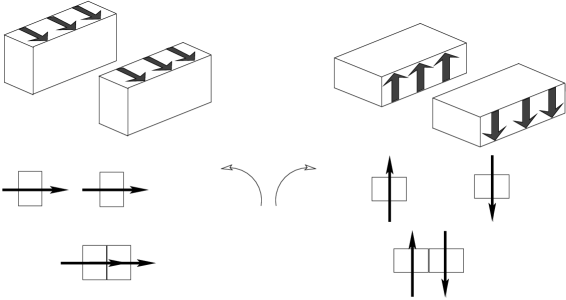
Figure 2: The magnets attracting each other. The dipol directions shown by arrows.

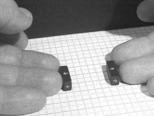
(a)

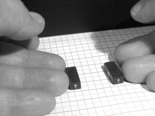
(b)

Figure 3: The magnets repelling each other are kept in position by fingers until the friction outweighs the repulsion (the dipole directions shown by arrows): (a) the parallel components have opposite direction, the stronger repulsion is felt against the friction to the distance of about five marks on the paper; (b) the perpendicular or upright components have the same direction, the weaker repulsion is felt against the friction to only about four marks on the paper.

3 The magic angle

The magic angle is used usually for the configuration where the two dipoles do not interact, i.e. it becomes zero. It can happen in the case that the two dipoles are parallel, one is placed in the origin, both point in ”the z-direction” while their connecting

Figure 4: The magic angle in the simplest configuration

vector’s polar angle $\theta$ defines the parallel and perpendicular components as

$${m}_{1\perp}={m}_{1}\sin\theta\ \ \ \ \ \ {m}_{1\|}={m}_{1}\cos\theta\ \ \ \ \ \$$ (5)

and the same for the second dipole ${m}_{2}$. Since the dipoles are parallel, the scalar products in the paranthesis reduce to

$${m}_{1\perp}{m}_{2\perp}-2{m}_{1\|}{m}_{2\|}$$ (6)

and this gives the condition for the magic angle

$$\sin^{2}\theta-2\cos^{2}\theta=0\ \ \ \ \ \ i.e.\ \ \ \ \ \ \tan\theta=\sqrt{2}$$ (7)

This gives the magic angle 54.74 degrees. In the literature this angle is usually derived from the original formula where number 3 appears which leads simply to the condition $3\cos^{2}\theta=1$ giving naturally the same magic angle.

4 The field lines of a dipole

The formula for the strength of magnetic field of the dipole ${\mathbf{m}}$ placed at the origin is

$${\mathbf{B}}({\mathbf{r}})=\frac{C}{r^{3}}\left(3\left({\mathbf{m}}\cdot\frac{{\mathbf{r}}}{r}\right)\frac{{\mathbf{r}}}{r}-{\mathbf{m}}\right)=\frac{C}{r^{3}}\left(3\left({\mathbf{m}}\cdot\hat{{\mathbf{r}}}\right)\hat{{\mathbf{r}}}-{\mathbf{m}}\right)$$ (8)

and it invites to similar rewriting, as

$${\mathbf{B}}({\mathbf{r}})=\frac{C}{r^{3}}\left(2{\mathbf{m}}_{\|}-{\mathbf{m}}_{\perp}\right)$$ (9)

This is again much simpler, and leads to the following suggestions for the visualizations of the field.

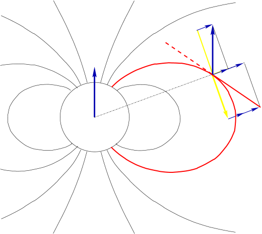
Figure 5: How to construct the field lines for the field of a an electric or magnetic dipole. The unit vector of in the dipole direction is decomposed into components parallel and perpendicular to the position vector. Then twice the parallel and once negative of the perpendicular components are added to give the direction of the field, i.e. the tangential line to the field line in the given position.

This is the prescription:

• Draw the dipole vector. Make the line to a point in plane

• Transfer the dipole vector and decompose it in components along and perpendicular to the connecting line

• Add together the twice the projection along the position vector and add the reverse (negative) of the perpendicular part. This gives the tangential line.

• Move along this direction - and start the next point

This makes fast constructins in e.g. matlab possible. (Note: if somebody had the same idea of rewriting as presented here, a natural place to look for it would probably be in the source files of simple graphics for field lines.)

The magnetic field of the dipole is also discussed at the physics part of Eric Weisstein’s science encyclopedia at Wolfram Research pages (ref. [5]). Here we have found the only place on the web which does not contain the factor 3, but factor 2 as in our present discussed formula (but the entry is very brief with no discussion). The two formulae there read

$${\mathbf{B}}({\mathbf{r}})=\frac{3\left({\mathbf{m}}\cdot{\mathbf{r}}\right){\mathbf{r}}-{\mathbf{m}}r^{2}}{r^{5}}=\frac{m}{r^{3}}\left(2\cos\theta\hat{{\mathbf{r}}}+\sin\theta\hat{\mathbf{\theta}}\right)$$ (10)

Here $\hat{{\mathbf{r}}}$ and $\hat{\theta}$ are unit vectors along the position vector and perpendicular to it, respectively. Due to their sign convention the minus sign essential in our discussion is unfortunately turned into a plus sign and the entry is too brief to include any interpretation. Note also that the units used are not specified. Fortunately, when compiling the final version of this paper we were given a reference to a published discussion in ref. [6] which includes correct units and a short discussion, but still without any interpretation along the lines of this paper.

5 Taylor expansion derivation of the electric dipole-dipole interaction

The purpose of this section is to demonstrate how a very straightforward treatment of the electric dipole-dipole interaction from the model of two pairs of charges shown in figure 6 leads directly to the standard dipole-dipole formula of equation 1. As is well known, the dipole formula is obtained in a limiting process, where the displacements are let to tend to zero while the the product of charge and displacement, the dipole moment, is kept constant.

The Coulomb interaction between the two pairs of charges can be written as (now we leave the units out alltogether)

$$-\frac{q^{2}}{|{\mathbf{r}}_{12}+{\mathbf{d}}_{2}-{\mathbf{d}}_{1}|}-\frac{q^{2}}{|{\mathbf{r}}_{12}-{\mathbf{d}}_{2}+{\mathbf{d}}_{1}|}+\frac{q^{2}}{|{\mathbf{r}}_{12}+{\mathbf{d}}_{2}+{\mathbf{d}}_{1}|}+\frac{q^{2}}{|{\mathbf{r}}_{12}-{\mathbf{d}}_{2}-{\mathbf{d}}_{1}|}\ \ \ \ \$$ (11)

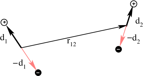
Figure 6: Deriving dipole-dipole potential using Taylor formula. Vectors shown by arrows.

To obtain the formula for dipole-dipole interaction we need to consider a case where ${r}_{12}\gg d_{1}$ and ${r}_{12}\gg d_{1}$. Up to the second term in Taylor expansion for 2-variables:

$$f(x+\Delta x,y+\Delta y)=f(x,y)+\left(f_{x}(x,y)\Delta x+f_{y}(x,y)\Delta y\right)+$$

$$\left.\ldots+\frac{1}{2!}\left[f_{{xx}}(x,y)(\Delta x)^{2}+2f_{{xy}}(x,y)\Delta x\Delta y+f_{{yy}}(x,y)(\Delta y)^{2}\right)\right]$$

In vector notation

$$f({\mathbf{r}}+{\mathbf{d}})=f({\mathbf{r}})+({\mathbf{d}}\cdot\nabla)({\mathbf{r}})+\frac{1}{2!}{\mathbf{d}}\cdot\left[({\mathbf{d}}\cdot\nabla)(\nabla f(r))\right]$$

The first order terms disappear due to the symmetry of the terms, thus we only need to consider the second order terms.

The $f(x)$ is

$$\frac{1}{r}=\frac{1}{\sqrt{x^{2}+y^{2}}}$$

thus we wish to obtain the vector formula for ${\mathbf{d}}=(\Delta x,\Delta y)$ from the very simple non-vector notation

$$\frac{\partial^{2}}{\partial x_{i}\partial x_{j}}\left(\frac{1}{\sqrt{x^{2}+y^{2}}}\right)=\frac{\partial}{\partial x_{i}}\left[\frac{\partial}{\partial x_{j}}\left(\frac{1}{\sqrt{x^{2}+y^{2}}}\right)\right]=\frac{\partial}{\partial x_{i}}\left[\frac{-x_{j}}{\left(\sqrt{x^{2}+y^{2}}\right)^{3}}\right]$$ (12)

$$= \left[\frac{-1}{\left(\sqrt{x^{2}+y^{2}}\right)^{3}}\frac{\partial x_{j}}{\partial x_{i}}-x_{j}\frac{\partial}{\partial x_{i}}\left(\frac{1}{\left(\sqrt{x^{2}+y^{2}}\right)^{3}}\right)\right]$$

$$= \left[\frac{-1}{\left(\sqrt{x^{2}+y^{2}}\right)^{3}}\delta_{{ij}}+3x_{j}\left(\frac{x_{i}}{\left(\sqrt{x^{2}+y^{2}}\right)^{5}}\right)\right]$$

From this formula it is then not difficult to show, comparing with the above vector form that Taylor expansion of

$$-\frac{q^{2}}{|{\mathbf{r}}_{12}+{\mathbf{d}}_{2}-{\mathbf{d}}_{1}|}-\frac{q^{2}}{|{\mathbf{r}}_{12}-{\mathbf{d}}_{2}+{\mathbf{d}}_{1}|}+\frac{q^{2}}{|{\mathbf{r}}_{12}+{\mathbf{d}}_{2}+{\mathbf{d}}_{1}|}+\frac{q^{2}}{|{\mathbf{r}}_{12}-{\mathbf{d}}_{2}-{\mathbf{d}}_{1}|}$$

where (with ${\mathbf{n}_{1}}$ and ${\mathbf{n}_{2}}$ the direction unit vectors of the charge displacements in each dipole)

$${\mathbf{d}}_{1}=\frac{d}{2}{\mathbf{n}}_{1}\ \ \ \ \ \ \ {\mathbf{d}}_{2}=\frac{d}{2}{\mathbf{n}}_{2}.$$

With the definitions of the dipole moments (note that the product $qd$ gives the size of the dipole moment, which is kept constant in the limiting process, meaning that while $d$ approaches zero, the charges $q$ must grow correspondingly)

$${\mathbf{m}}_{1}=(qd){\mathbf{n}}_{1}\ \ \ \ \ \ \ {\mathbf{m}}_{2}=(dq){\mathbf{n}}_{2}$$

the above derivation in equations 12 leads directly to form of the starting formula 1.

$$\frac{1}{r_{12}^{\ \ 3}}\left[{\mathbf{m}}_{1}\cdot{\mathbf{m}}_{2}-\frac{3\left({\mathbf{m}}_{1}\cdot{\mathbf{r}}_{12}\right)\left({\mathbf{m}}_{2}\cdot{\mathbf{r}}_{12}\right)}{r_{12}^{\ \ 2}}\right]$$

The above derivation possibly explains why the usual formula is a straightforward choice, and there seems no need to transform the expression. This might have contributed to a general acceptance of the standard formula as the only reasonable choice. Also, the standard formula does not need any additional definition of the perpendicular components and appears as a most general coordinate system independent expression. Hopefully, this paper has shown that there indeed are some advantages in transformations and rearrangements of the standard formula for dipole-dipole interaction as well as the related vector fields.

6 Conclusion

The dipole-dipole interaction formula has been shown to contain a possibility to be transformed to a much more intuitive form. We have shown the applications which are suitable for teaching and illustrations. It appears however that also in research applications the insight provided by this simple transformation of the standard formula might contribute to more intuitive presentations and discussions. The transformation itself is really very elementary and it is thus rather surprizing that it has not been discussed earlier. In fact, while preparing the final version of this paper, we have by chance found a new textbook of Quantum Chemistry [7] showing a version similar to ours here, but in a component form. This form appears to the author to be unsafely coordinate system dependent and is thus immediately replaced by ”waterproof” form of which is the standard of equation 1.

References

References

- [1] J D Jackson 1997Classical Electrodynamics (Reading, MA: Addison-Wesley)
- [2] http://en.wikipedia.org/wiki/Magnetic_dipole-dipole_interaction wikipedia: Magnetic dipole-dipole interaction
- [3] http://en.wikipedia.org/wiki/Magic_angle wikipedia: Magic angle
- [4] http://en.wikipedia.org/wiki/Dipole wikipedia: Dipole
- [5] http://scienceworld.wolfram.com/physics/MagneticDipole.html Eric Weisstein: Science World: Field of magnetic dipole
- [6] N. Gauthier, Am. J. Phys. 69 (2001) 384 Comment on ”Field pattern of a magnetic dipole”…
- [7] L. Piela 2007, Ideas of Quantum Chemistry (Amsterdam, The Netherlands: Elsevier), page 701, Section 13.6.4