CAVENDISH-HEP-2009-09, DAMTP-2009-42, LPSC-09-114, SCUPHY-TH-09003

Neutralino Reconstruction at the LHC from Decay-frame Kinematics

Z. Kang and N. Kersting

Physics Department, Sichuan University

Chengdu, Sichuan Province, P.R. China 610065

S. Kraml

Laboratoire de Physique Subatomique et de Cosmologie (LPSC)

UJF Grenoble 1, CNRS/IN2P3, 53 Avenue des Martyrs, F-38026 Grenoble, France

A.R. Raklev

DAMTP, Wilberforce Road, Cambridge, CB3 0WA, UK

Cavendish Laboratory, JJ Thomson Avenue, Cambridge, CB3 0HE, UK

M.J. White

Cavendish Laboratory, JJ Thomson Avenue, Cambridge, CB3 0HE, UK

Decay-frame Kinematics (DK) has previously been introduced as a technique to reconstruct neutralino masses from their three-body decays to leptons. This work is an extension to the case of two-body decays through on-shell sleptons, with Monte Carlo simulation of LHC collisions demonstrating reconstruction of neutralino masses for the SPS1a benchmark point.

1 Introduction

The Large Hadron Collider (LHC) at CERN, Geneva, is expected to provide direct evidence for any New Physics beyond the Standard Model (SM) at the TeV energy scale. The properties of these particles may shed light on the origin of electroweak symmetry breaking and the nature of dark matter, and give clues to a more fundamental theory of Nature. To explain the deficiencies of the SM, a large variety of theories has been put forward, and it is only by carefully measuring the properties of any new particles that one will be able to discriminate between them. Chief amongst these properties are the masses of the new particles.

Many of these new theories (e.g., supersymmetry and extra dimensions) contain a stable weakly interacting massive particle that will only be ‘visible’ in an LHC detector as missing energy. Such particles are natural dark matter candidates by virtue of their interactions, but pose problems for mass measurements at hadron colliders since one cannot in general reconstruct the kinematics of an event in which these particles are produced. To worsen the problem, the parton–parton interactions in the collider have by their very nature an unknown center of mass energy.

In the literature a number of techniques has been developed to get around this problem. These fall into two general classes: those that perform a fit to or set a limit on masses using information from the entire event sample, and those which rely exclusively on events near the endpoint of a kinematic distribution. Belonging to the first class are “Mass-Shell Techniques” (MSTs), represented by the work done in [1, 2], [3, 4, 5] and [6], which depend on maximizing the solvability of assumed mass-shell constraints in a given sample of events. This has been shown to be very effective if enough such constraints are available. Also belonging to this class are techniques which work with extrema of a “transverse mass” variable, e.g., $m_{T2}$ [8, 9, 10, 11, 12, 13, 14], and techniques which look at the shape of complete invariant mass distributions [15, 16, 17, 18, 19]. Much research has recently become focused in these areas.

The second class of mass reconstruction techniques most notably includes the traditional kinematic endpoint method [20, 21, 22, 23, 24, 25, 26, 27, 28], where the endpoints of various invariant mass distributions can be matched to analytical functions of the unknown masses, that in turn can be inverted to solve for the same masses in suitably long decay chains. Such methods have been studied for over a decade already, and would seem to have been largely explored for the simplest, and most probable, decay chains in popular theories such as the Minimal Supersymmetric Standard Model (MSSM). However, there is more to be done with events near an endpoint as demonstrated recently in [29]: here a Decay-frame Kinematics (DK) technique utilizes the fact that events at a kinematic endpoint can have exactly-known kinematics in terms of production angles and energies of all particles in the assumed decay chain. Events near an endpoint will thus have approximately known decay-frame kinematics, which allows one to constrain and solve for unknown masses. In [29] this was demonstrated for the case of neutralino three-body decays through off-shell sleptons to lepton pairs plus missing energy carried away by the lightest supersymmetric particle (LSP), the lightest neutralino, e.g. $\tilde{\chi}_{2}^{0}\to\ell^{+}\ell^{-}\tilde{\chi}_{1}^{0}$. The on-shell case was deferred to a future work — this work.

In the following we will demonstrate the use of DK in the case of on-shell neutralino decays, i.e. $\tilde{\chi}_{i}^{0}\to\tilde{\ell}^{\pm}\ell^{\mp}\to\ell^{+}\ell^{-}\tilde{\chi}_{1}^{0}$, though it should be stressed that the technique demonstrated can be applied to any similar cascade decay process arising in any New Physics model. Section 2 begins with a review of the off-shell case, demonstrating its application at a NMSSM parameter point. Section 3 then discusses the main new development of this paper, the generalisation of the DK technique to the on-shell case, where it is found that several subtleties emerge beyond what was found for the comparatively simple off-shell case; we further present a Monte Carlo (MC) study of the mSUGRA SPS1a benchmark point [30], where the DK technique proves quite capable of reconstructing the relevant neutralino masses from $\tilde{\chi}_{2}^{0}\tilde{\chi}_{2}^{0}$ decays. Section 4 gives our conclusions.

2 Off-Shell Decays

We begin with a brief review of the DK technique applied to the case of neutralino three-body decays. For a more complete treatment, see [29]. We consider production of neutralino pairs in the MSSM which undergo three-body decays to electrons, muons, and $\tilde{\chi}_{1}^{0}$ (the LSP):

$$pp\to\mathbb{X}\to\mathbb{X}^{\prime}+\tilde{\chi}_{i}^{0}(\to e^{+}e^{-}\tilde{\chi}_{1}^{0})~{}\tilde{\chi}_{j}^{0}(\to\mu^{+}\mu^{-}\tilde{\chi}_{1}^{0}),$$ (1)

where $\mathbb{X}$ represents either a $Z^{*}$ or any MSSM production channel via a Higgs ($H^{0}$ or $A^{0}$) or cascade from gluino/squark pair-production, while $\mathbb{X}^{\prime}$ are SM states potentially produced in association, relevant in this context only for the measurement of missing momentum. The physical observables of interest from one event thus consist of four leptonic four-momenta $p_{e^{\pm},\mu^{\pm}}$, from which we may construct the usual di-lepton invariant masses, $M_{ee}$ and $M_{\mu\mu}$, and missing momentum in two transverse directions, assumed equal to the sum of the two LSPs’ transverse momenta, $p_{\chi,\chi^{\prime}}^{T}$. If we happen to have an event where both the invariant masses $M_{ee}$ and $M_{\mu\mu}$ are maximal, as shown in Fig. 1a, it will be subject to the system of constraints (hereafter we abbreviate $m_{i}\equiv m_{\widetilde{\chi}_{i}^{0}}$)

$$M_{ee}^{\max} = m_{i}-m_{1},$$ (2)

$$M_{\mu\mu}^{\max} = m_{j}-m_{1},$$ (3)

$$\vec{p}_{e^{+}}^{~{}\prime}+\vec{p}_{e^{-}}^{~{}\prime} = 0,$$ (4)

$$\vec{p}_{\mu^{+}}^{~{}\prime}+\vec{p}_{\mu^{-}}^{~{}\prime} = 0,$$ (5)

$$(\vec{p}_{\chi}+\vec{p}_{\chi^{\prime}})^{T} = \not\!{\vec{p}}^{~{}T}~{}\mathrm{(observed),}$$ (6)

where leptonic momenta are written in the rest frame of the respective parent neutralino, and $\vec{p}_{e^{\pm}}^{~{}\prime}=\mathbf{\Lambda}_{1}\vec{p}_{e^{\pm}}$ and $\vec{p}_{\mu^{\pm}}^{~{}\prime}=\mathbf{\Lambda}_{2}\vec{p}_{\mu^{\pm}}$ define the appropriate Lorentz transformations $\mathbf{\Lambda}_{1,2}$ from the lab frame. This system gives ten equations for the nine unknowns, the velocities $\vec{\beta}_{1,2}$ and the masses $m_{1,i,j}$, allowing us to actually overconstrain the masses $m_{1,i,j}$. The $\vec{\beta}_{1,2}$ which satisfy (4) and (5), making the total momentum of each lepton pair zero, are uniquely given by

$$\vec{\beta}_{1}=\frac{\vec{p}_{e^{+}}+\vec{p}_{e^{-}}}{E_{e^{+}}+E_{e^{-}}}\quad{\rm and}\quad\vec{\beta}_{2}=\frac{\vec{p}_{\mu^{+}}+\vec{p}_{\mu^{-}}}{E_{\mu^{+}}+E_{\mu^{-}}}.$$ (7)

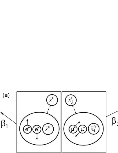
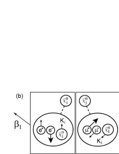
Figure 1: (a) Neutralino three-body decays with maximal $M_{ee}$ and $M_{\mu\mu}$: though the decaying $\tilde{\chi}_{i,j}^{0}$ may be moving with any velocity $\beta_{1,2}$ in the lab frame, in each respective decay frame the leptons have equal and opposite momenta while the $\tilde{\chi}_{1}^{0}$ (LSP) is at rest. (b) If the $\tilde{\chi}_{i,j}^{0}$ has a two-body decay via on-shell sleptons, the LSPs are no longer stationary in the neutralino decay frame, but have momenta $K_{i,j}$ collinear with the leptons’ momenta.

Now, because of the condition that $M_{ee}$ and $M_{\mu\mu}$ are maximal, the corresponding $\mathbf{\Lambda}_{1,2}$, which take the $e^{+}e^{-}\tilde{\chi}_{1}^{0}$ and $\mu^{+}\mu^{-}\tilde{\chi}_{1}^{0}$ systems to their respective $\tilde{\chi}_{i,j}^{0}$ rest frames, also bring each $\tilde{\chi}_{1}^{0}$ to rest. Thus their four-momenta in these frames must be $(m_{1},\vec{0})$, which, when inverse-Lorentz-transformed by $\mathbf{\Lambda}_{1,2}^{-1}$, giving $(m_{1}\gamma_{1,2}~{},m_{1}(\vec{\beta}\gamma)_{1,2})$, have to agree with the observed missing momentum $\not\!\vec{p}^{~{}T}$; this matching condition along each transverse direction (say $\hat{x}$ and $\hat{y}$) then gives two independent determinations of $m_{1}$:

$$m_{1}^{\prime}=\frac{\not\!{p}_{x}}{(\beta_{x}\gamma)_{1}+(\beta_{x}\gamma)_{2}}\quad{\rm and}\quad m_{1}^{\prime\prime}=\frac{\not\!{p}_{y}}{(\beta_{y}\gamma)_{1}+(\beta_{y}\gamma)_{2}}.$$ (8)

Since we are assuming that both $M_{ee}$ and $M_{\mu\mu}$ are precisely maximal — the perfect event of Fig. 1a — we should get $m_{1}^{\prime}=m_{1}^{\prime\prime}=m_{1}$ from such an event. In practice of course, we can only expect to find an event within some neighborhood $\epsilon$ of the endpoints, $M_{ee,\mu\mu}=M_{ee,\mu\mu}^{\max}\pm\epsilon$, in which case one finds that $m_{1}^{\prime}$ and $m_{1}^{\prime\prime}$ are offset by ${\mathcal{O}}(\sqrt{2\epsilon m_{1}})$ from $m_{1}$ [29]. One might then expect that applying (7) and (8) to a sample of events near the endpoint should give a distribution of $m_{1}^{\prime}$ and $m_{1}^{\prime\prime}$ peaked near $m_{1}$ with a spread determined by sample purity.

Here, to lend further support to the generality of the above technique, let us demonstrate its application to the rather challenging example of an NMSSM (Next-to-Minimal Supersymmetric Standard Model) scenario described in [19]. This has a supersymmetric particle spectrum containing five neutralinos, the lightest of which is 99% singlino, and a generic feature of the parameter space that gives the correct dark matter density is a significant degeneracy between the singlino and second lightest neutralino mass. This gives rise to copious production of soft lepton pairs with small invariant masses, $M_{\ell\ell}\;\raisebox{-3.87495pt}{$\textstyle\stackrel{{\scriptstyle\textstyle<}}{{\sim}}$}\;10$ GeV, from the three-body decay $\tilde{\chi}_{2}^{0}\to\ell^{+}\ell^{-}\tilde{\chi}_{1}^{0}$. For more details on this scenario see [19].

We study the benchmark “Point A” of that paper, a point which has $M_{\ell\ell}^{\max}=9.7$ GeV and $m_{1}=105.4$ GeV, using the same MC setup and fast detector simulation as in [19]. For details of the simulation see also Section 3 of the present paper. To isolate signal events of the type (1), we place the following cuts on our events:

• Require missing transverse energy $\not\!\!E_{T}>100$ GeV.

• Require at least two hard jets with $p_{T}>150,\,100$ GeV.

• Require four isolated leptons with flavor structure $e^{+}e^{-}\mu^{+}\mu^{-}$ and $p_{T}>7\,(4)$ for $e$ $(\mu)$. All such leptons must pass the lepton efficiency cuts employed in [19] modeled on full simulation results given in [31].

From the surviving events we construct a wedgebox plot of the di-electron versus the di-muon invariant mass, for a number of events equivalent to 30 fb^-1 of statistics at the LHC. The result is seen in Fig. 2a, showing a clear box-like structure at $M_{ee,\mu\mu}\sim 10$ GeV, the endpoint of the di-lepton invariant mass distribution for the $\tilde{\chi}_{2}^{0}$ decay.

Choosing a sampling region in a rather generous neighborhood of the endpoint, $M_{\ell\ell}=10\pm 4$ GeV gives ${\mathcal{O}}(100)$ events. We now apply Eqs. (7) and (8) to each of these, demanding that $m_{1}^{\prime}$ and $m_{1}^{\prime\prime}$ agree to within 20%. Although only about 20 events survive this criterion, the resulting $m_{1}$ distribution can be seen in Fig. 2b to peak quite prominently slightly below the nominal value of $m_{1}=105.4$ GeV. The systematic error of the method is seen to be comparable to the estimate made earlier.

With higher statistics, this allows us to determine the absolute LSP mass to rather good precision. The results for 300 fb^-1 of data are shown in Fig. 2c. Here we narrow down our sampling region to $\epsilon=1$ GeV from the wedgebox edge. With a Gaussian distribution we obtain a best fit value of $m_{1}=98.2\pm 3.9$ GeV with $\chi^{2}/{\rm ndf}=0.41$.

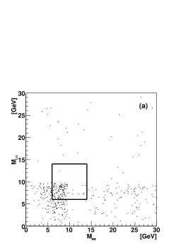
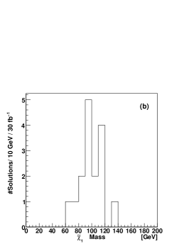
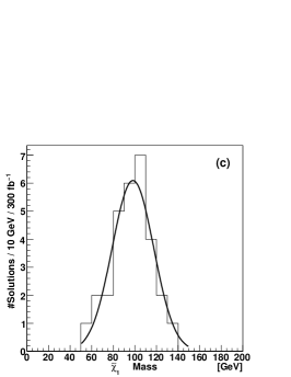
Figure 2: (a) Wedgebox plot for 30 fb^-1 of integrated LHC luminosity for “Point A” of [19]. (b) The $\tilde{\chi}_{1}^{0}$ mass distribution for events sampled from the boxed region in (a). We see a peak in rough agreement with the nominal value of $m_{1}=105.4$ GeV. (c) Same as (b) but for 300 fb^-1 and $\epsilon=1$ GeV.

3 On-Shell Decays

3.1 Kinematics

Let us now continue to the main focus of this paper, i.e. the added complications that arise when the neutralinos decay through on-shell intermediate sleptons:

$$\mathbb{X}\to\mathbb{X}^{\prime}+\tilde{\chi}_{i}^{0}\tilde{\chi}_{j}^{0}(\to e^{\pm}\tilde{e}^{\mp}\mu^{\pm}\tilde{\mu}^{\mp}\to e^{+}e^{-}\mu^{+}\mu^{-}\tilde{\chi}_{1}^{0}\tilde{\chi}_{1}^{0}).$$ (9)

When $M_{ee}$ and $M_{\mu\mu}$ are maximal, as illustrated in Fig. 1b, two-body kinematics gives the following system of constraints:

$$M_{ee}^{\max} = m_{i}\sqrt{1-(m_{s}/m_{i})^{2}}\sqrt{1-(m_{1}/m_{s})^{2}},$$ (10)

$$M_{\mu\mu}^{\max} = m_{j}\sqrt{1-(m_{s}/m_{j})^{2}}\sqrt{1-(m_{1}/m_{s})^{2}},$$ (11)

$$\vec{p}_{e^{+}}^{~{}\prime} \parallel -\vec{p}_{e^{-}}^{~{}\prime},$$ (12)

$$\vec{p}_{\mu^{+}}^{~{}\prime} \parallel -\vec{p}_{\mu^{-}}^{~{}\prime},$$ (13)

$$|\vec{p}_{e^{+}}^{~{}\prime}+\vec{p}_{e^{-}}^{~{}\prime}| = \left|\frac{m_{s}^{4}-m_{i}^{2}m_{1}^{2}}{2m_{i}m_{s}^{2}}\right|\equiv K_{i},$$ (14)

$$|\vec{p}_{\mu^{+}}^{~{}\prime}+\vec{p}_{\mu^{-}}^{~{}\prime}| = \left|\frac{m_{s}^{4}-m_{j}^{2}m_{1}^{2}}{2m_{j}m_{s}^{2}}\right|\equiv K_{j},$$ (15)

$$(\vec{p}_{\chi}+\vec{p}_{\chi^{\prime}})^{T} = \not\!\vec{p}^{~{}T}~{}\mathrm{(observed)},$$ (16)

where we have assumed a common slepton mass $m_{s}=m_{\tilde{e}}=m_{\tilde{\mu}}$. See the Appendix for details of the derivation. The antiparallel conditions (12) and (13) force $\vec{\beta}_{1,2}$ to be in the planes of the respective leptons, so there are really only four boost parameters to find; adding the unknown masses $m_{1,i,j,s}$ to this gives eight unknowns which can thus be solved for by the eight constraints (10)–(16). In principle, if one were handed an event of the type in Fig. 1b, one could numerically apply (10)–(16), scanning over the eight-dimensional space of unknowns for a solution. Needless to say, this is not the most practical approach, nor particularly enlightening as to the nature of any solution which might be found.

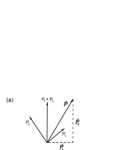
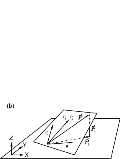
Figure 3: (a) When lepton pairs from the decay chain $\tilde{\chi}_{i}^{0}\to\ell^{\pm}\tilde{\ell}^{\mp}\to\ell^{+}\ell^{-}\tilde{\chi}_{1}^{0}$ have maximal invariant mass, their momenta $P_{1,2}$ in the lab frame are coplanar with the LSP momentum $\not\!P$. (b) The LSP’s longitudinal momentum $\not\!P_{L}$ can be found by the condition that $\not\!P$ is in the plane of the leptons.

Instead, we will proceed temporarily as if we already knew the individual $\vec{p}_{\chi,\chi^{\prime}}^{~{}T}$ as opposed to just their sum (16). Consider, then, just one of the neutralino decays, say $\tilde{\chi}_{i}^{0}\to e^{\pm}\tilde{e}^{\mp}\to e^{+}e^{-}\tilde{\chi}_{1}^{0}$. In the $\tilde{\chi}_{i}^{0}$ rest frame, the leptons’ three-momenta ($\equiv\vec{P}_{1,2}^{\prime}$) are back-to-back and collinear with the LSP’s three-momentum ($\equiv\vec{\not\!{P}}^{\prime}$); thus, in the lab frame where $\tilde{\chi}_{i}^{0}$ has a velocity $\vec{\beta_{1}}$, the boosted momenta $\vec{P}_{1}$, $\vec{P}_{2}$, and $\vec{\not\!{P}}$ lie in the same plane (see Fig. 3a). Looking at this the other way round, $\vec{\beta_{1}}$ is the Lorentz boost which makes the observed lepton momenta antiparallel and fixes the magnitude of their sum to be $K_{i}$ — which we a priori don’t know at this point — i.e.  constraints (12) and (14). Necessarily, $\vec{\beta_{1}}$ must be in the observed leptons’ plane. If we choose a basis in this plane $(\hat{p}_{\|},~{}\hat{p}_{\bot})$ parallel/perpendicular to the total leptonic momentum $\vec{P}\equiv\vec{P}_{1}+\vec{P}_{2}$, then the boost $\vec{\beta_{1}}=(\beta_{\|},~{}\beta_{\bot})$ must satisfy three sets of constraints:

1. The transformed leptonic momenta must be antiparallel:

   $$\vec{P}_{1}^{\prime}\cdot\vec{P}_{2}^{\prime}=-|\vec{P}_{1}^{\prime}||\vec{P}_{2}^{\prime}|,$$ (17)

   where the transformed four-vectors are given in terms of the boost by

   $$\left(\begin{array}[]{c}E_{1,2}^{\prime}\\ P_{1,2}^{\prime\|}\\ P_{1,2}^{\prime\bot}\\ \end{array}\right)=\left(\begin{array}[]{ccc}\gamma&-\beta_{\|}\gamma&-\beta_{\bot}\gamma\\ -\beta_{\|}\gamma&1+(\gamma-1)\frac{\beta_{\|}^{2}}{\beta^{2}}&(\gamma-1)\frac{\beta_{\|}\beta_{\bot}}{\beta^{2}}\\ -\beta_{\bot}\gamma&(\gamma-1)\frac{\beta_{\|}\beta_{\bot}}{\beta^{2}}&1+(\gamma-1)\frac{\beta_{\bot}^{2}}{\beta^{2}}\\ \end{array}\right)\left(\begin{array}[]{c}E_{1,2}\\ P_{1,2}^{\|}\\ P_{1,2}^{\bot}\\ \end{array}\right),$$ (18)

   with $\beta^{2}\equiv\beta_{\|}^{2}+\beta_{\bot}^{2}$ and $\gamma\equiv(1-\beta^{2})^{-1/2}$.

2. The transformed total leptonic momentum must equal $\vec{K}_{i}=(K_{i}^{\|},~{}K_{i}^{\bot})$:

   $$\left(\begin{array}[]{c}E^{\prime}\\ K_{i}^{\|}\\ K_{i}^{\bot}\\ \end{array}\right)=\left(\begin{array}[]{ccc}\gamma&-\beta_{\|}\gamma&-\beta_{\bot}\gamma\\ -\beta_{\|}\gamma&1+(\gamma-1)\frac{\beta_{\|}^{2}}{\beta^{2}}&(\gamma-1)\frac{\beta_{\|}\beta_{\bot}}{\beta^{2}}\\ -\beta_{\bot}\gamma&(\gamma-1)\frac{\beta_{\|}\beta_{\bot}}{\beta^{2}}&1+(\gamma-1)\frac{\beta_{\bot}^{2}}{\beta^{2}}\\ \end{array}\right)\left(\begin{array}[]{c}E\\ P\\ 0\\ \end{array}\right),$$ (19)

   where the components $(K_{i}^{\|},K_{i}^{\bot})$ are also unknown at this point.

3. The inverse-Lorentz-boosted LSP four-momentum must satisfy

   $$\left(\begin{array}[]{c}\hbox to0.0pt{\hbox to7.95831pt{\hfil/\hfil}\hss}E\\ \hbox to0.0pt{\hbox to7.80904pt{\hfil/\hfil}\hss}P_{\|}\\ \hbox to0.0pt{\hbox to7.80904pt{\hfil/\hfil}\hss}P_{\bot}\\ \end{array}\right)=\left(\begin{array}[]{ccc}\gamma&\beta_{\|}\gamma&\beta_{\bot}\gamma\\ \beta_{\|}\gamma&1+(\gamma-1)\frac{\beta_{\|}^{2}}{\beta^{2}}&(\gamma-1)\frac{\beta_{\|}\beta_{\bot}}{\beta^{2}}\\ \beta_{\bot}\gamma&(\gamma-1)\frac{\beta_{\|}\beta_{\bot}}{\beta^{2}}&1+(\gamma-1)\frac{\beta_{\bot}^{2}}{\beta^{2}}\\ \end{array}\right)\left(\begin{array}[]{c}\sqrt{K_{i}^{2}+m_{1}^{2}}\\ -K_{i}^{\|}\\ -K_{i}^{\bot}\\ \end{array}\right).$$ (20)

After some algebra, see the Appendix, these constraints are found to uniquely determine the unknown boost $(\beta_{\|},~{}\beta_{\bot})$ in terms of the known lab frame leptonic momenta and unknown LSP momenta:

$$\beta_{\|}=\frac{P}{E(1+\alpha x)}\quad{\rm and}\quad\beta_{\bot}=\alpha\beta_{\|},$$ (21)

where

$$\alpha\equiv\frac{\hbox to0.0pt{\hbox to7.80904pt{\hfil/\hfil}\hss}P_{\bot}}{\hbox to0.0pt{\hbox to7.80904pt{\hfil/\hfil}\hss}P_{\|}+P}\quad{\rm and}\quad x\equiv\frac{P(P_{1}^{\bot}-P_{2}^{\bot})(P_{2}^{\|}-P_{1}^{\|})}{2E(E_{1}P_{2}^{\|}+E_{2}P_{1}^{\|})}.$$

Thus, knowing the leptonic momenta and missing momentum from the LSP determines $x$ and $\alpha$, hence $\vec{\beta}_{1}$ and all the kinematic information in the event. At first glance this may seem useless since we can only have knowledge of the transverse component of $\vec{\hbox to0.0pt{\hbox to7.80904pt{\hfil/\hfil}\hss}P}$ in the lab coordinate system, $\vec{\hbox to0.0pt{\hbox to7.80904pt{\hfil/\hfil}\hss}P_{T}}$, and there are two LSPs that contribute to the measured total missing momentum.

However, given the transverse component of the LSP momentum we can in fact reconstruct the longitudinal component $\vec{\hbox to0.0pt{\hbox to7.80904pt{\hfil/\hfil}\hss}P_{L}}$ by the following trick: since $\vec{\hbox to0.0pt{\hbox to7.80904pt{\hfil/\hfil}\hss}P}$ must lie in the plane of the leptons while $\vec{\hbox to0.0pt{\hbox to7.80904pt{\hfil/\hfil}\hss}P_{T}}$ is by definition in the transverse $\hat{x}$-$\hat{y}$ plane, $\vec{\hbox to0.0pt{\hbox to7.80904pt{\hfil/\hfil}\hss}P_{L}}$ must be of the precise size along $\hat{z}$ to bring $\vec{\hbox to0.0pt{\hbox to7.80904pt{\hfil/\hfil}\hss}P_{T}}+\vec{\hbox to0.0pt{\hbox to7.80904pt{\hfil/\hfil}\hss}P_{L}}$ into the leptons’ plane (see Fig. 3b), i.e. $(\vec{\hbox to0.0pt{\hbox to7.80904pt{\hfil/\hfil}\hss}P_{T}}+\vec{\hbox to0.0pt{\hbox to7.80904pt{\hfil/\hfil}\hss}P_{L}})\cdot(\vec{P}_{1}\times\vec{P}_{2})=0$, giving

$$\vec{\hbox to0.0pt{\hbox to7.80904pt{\hfil/\hfil}\hss}P}_{L}=-\frac{\hbox to0.0pt{\hbox to7.80904pt{\hfil/\hfil}\hss}P_{Tx}(P_{1y}P_{2z}-P_{1z}P_{2y})+\hbox to0.0pt{\hbox to7.80904pt{\hfil/\hfil}\hss}P_{Ty}(P_{1z}P_{2x}-P_{1x}P_{2z})}{P_{1x}P_{2y}-P_{1y}P_{2x}}\hat{z}.$$ (22)

With both $\vec{\hbox to0.0pt{\hbox to7.80904pt{\hfil/\hfil}\hss}P_{T}}$ and $\vec{\hbox to0.0pt{\hbox to7.80904pt{\hfil/\hfil}\hss}P_{L}}$ known we may immediately project $\vec{\hbox to0.0pt{\hbox to7.80904pt{\hfil/\hfil}\hss}P}$ into the basis $(\hbox to0.0pt{\hbox to7.80904pt{\hfil/\hfil}\hss}P_{\|},~{}\hbox to0.0pt{\hbox to7.80904pt{\hfil/\hfil}\hss}P_{\bot})$, compute $\alpha$ and insert into (21) to solve for the boosts. We can then use Eq. (19) to solve for $K_{i}^{\|}$ and $K_{i}^{\bot}$:

$$K_{i}^{\|}=P\left(\frac{\gamma+\alpha^{2}}{1+\alpha^{2}}-\frac{\gamma}{1+\alpha x}\right),\quad\quad K_{i}^{\bot}=\alpha P\left(\frac{\gamma-1}{1+\alpha^{2}}-\frac{\gamma}{1+\alpha x}\right),$$ (23)

which are also related by $K_{i}^{\bot}=\alpha(K_{i}^{\|}-P)$. We see that in the limit $\alpha\to 0$ both $K_{i}^{\|,\bot}\to 0$, and that also Eq. (21) correctly reduces to the off-shell result $\beta=P/E$.

Finally, the LSP mass can then be found from the energy component of Eq. (20):

$$m_{1}=\sqrt{\left(\frac{\hbox to0.0pt{\hbox to7.80904pt{\hfil/\hfil}\hss}P_{\|}}{\beta_{\|}\gamma}+\left(1+\frac{(\gamma-1)\beta_{\|}^{2}}{\beta^{2}}\right)\frac{K_{i}^{\|}}{\beta_{\|}\gamma}+\frac{(\gamma-1)\beta_{\bot}K_{i}^{\bot}}{\beta^{2}\gamma}\right)^{2}-{K_{i}^{\|}}^{2}-{K_{i}^{\bot}}^{2}},$$ (24)

which again reduces to the off-shell result of Eq. (8) when $K_{i}^{\|,\bot}\to 0$. The heavier neutralino mass follows from the energy component of (19) and energy conservation in its decay, i.e.

$$m_{i}=\sqrt{K_{i}^{2}+m_{1}^{2}}+\gamma E-\beta_{\|}\gamma P,$$ (25)

while the slepton mass is related to $m_{1}$ and $m_{i}$ by (10).

Finally, let us return to deal with the realistic situation where we know only the sum of the LSP momenta $(\vec{p}_{\chi}+\vec{p}_{\chi^{\prime}})^{T}$. From the discussion above, every assignment of $\not\!\vec{P}_{T}=\vec{p}_{\chi}^{~{}T}$ will yield a set of masses $\{m_{1}^{\prime},~{}m_{i}^{\prime},~{}m_{s}^{\prime}\}$ which satisfy (10), (12), and (14). Then the other LSP has its $\vec{p}_{\chi^{\prime}}^{~{}T}$ fixed as $\vec{p}_{\chi^{\prime}}^{~{}T}=\not\!\vec{p}^{~{}T}-\vec{p}_{\chi}^{~{}T}$, giving another set of masses $\{m_{1}^{\prime\prime},~{}m_{i}^{\prime\prime},~{}m_{s}^{\prime\prime}\}$ which satisfy (11), (13), and (15). Under the simplifying assumption that the event contains the process in (9) with $i=j$, we should clearly insist that at least $\{m_{1}^{\prime},~{}m_{i}^{\prime}\}\simeq\{m_{1}^{\prime\prime},~{}m_{i}^{\prime\prime}\}$ within some error (we reserve the possibility that $m_{s}^{\prime}\neq m_{s}^{\prime\prime}$). This, in principle, provides two constraints on our choice of the two components of $\vec{p}_{\chi}^{~{}T}$, i.e. the system (10)–(16) is solved.

Thus, in the end, we still have to resort to a numerical search for a solution to (10)–(16), but this is only over the two-dimensional space of one of the LSPs’ transverse momenta, $(p_{\chi}^{x},~{}p_{\chi}^{y})$. Nevertheless, it is not at all obvious that there won’t be multiple solutions with different $\{m_{1},~{}m_{i}\}$ within a given level of tolerance — and when one adds to this the same caveat as in the three-body case of picking events within some $\epsilon$ of the endpoint, as well as the effects of detector smearing and issues with backgrounds, it will have to fall to a MC simulation to test the practicality of the method.

3.2 Monte Carlo Test

We perform a Monte Carlo study by generating SUSY signal events for the SPS1a benchmark point [30] using PYTHIA 6.413 [32], and SM background events with HERWIG 6.510 [33, 34], interfaced to ALPGEN 2.13 [35] for the production of high jet multiplicities matched to parton showers and JIMMY 4.31 [36] for multiple interactions. The benchmark point is chosen mainly for the sake of comparison with results obtained with other mass reconstruction techniques, which we will comment more on in Section 4. The generated events are then put through a fast simulation of a generic LHC detector, AcerDET-1.0 [37], widely used to simulate analyses of high-$p_{T}$ physics at the LHC. This incorporates such detector effects as the deposition of energy in calorimeter cells, and the smearing of electron, photon, muon and hadronic cluster energies with parameterized resolutions. The AcerDET-1.0 isolation requirement for leptons is less than 10 GeV energy in a $R=0.2$ cone around the lepton and a minimum distance of $\Delta R=0.4$ from calorimetric clusters. The MC setup is essentially the same as in [19] and we refer the reader to that paper for more details. However, we point out that we use $p_{T}$ dependent lepton efficiencies based on full simulation studies published in [31].

All SUSY processes and relevant SM backgrounds are generated with a number of events corresponding to an integrated LHC luminosity of 300 fb^-1. The dominant type of neutralino pairs produced at SPS1a are $\tilde{\chi}_{2}^{0}\tilde{\chi}_{2}^{0}$; we will therefore concentrate on decays of the form $\tilde{\chi}_{2}^{0}(\to e^{+}e^{-}\tilde{\chi}_{1}^{0})~{}\tilde{\chi}_{2}^{0}(\to\mu^{+}\mu^{-}\tilde{\chi}_{1}^{0})$, and results in the previous section can be simplified somewhat by setting $i=j=2$, and in particular $K\equiv K_{i}=K_{j}$.

For this analysis we use the same set of cuts as for the NMSSM case in the previous Section, giving a signal size of roughly 470 events. Note the requirement of four isolated leptons with flavor structure $e^{+}e^{-}\mu^{+}\mu^{-}$ reduces most SM backgrounds to a negligible level[38]. Support for this in the context of a full simulation of the ATLAS detector is found in Higgs searches for the channel $h\to ZZ^{*}\to 4\ell$, e.g. discussed in [39, 40]. The remaining backgrounds of any importance are found to be $t\bar{t}$, $Zb\bar{b}$ and irreducible $Z^{(*)}Z$. We have simulated a large sample of $t\bar{t}$ events with up to two additional hard jets, and find no surviving events with the additional missing energy and jet cuts. The $Zb\bar{b}$ and $Z^{(*)}Z$ backgrounds are also expected to be very small after these cuts. However, because the $Z$ mass is sufficiently far from the dilepton edge, any remaining events from these backgrounds do not significantly influence the region of interest in the di-electron versus di-muon invarant mass plane, shown in the wedgebox plot of Fig. 4a.

The position of the edge of the box-like structure at $M_{\ell\ell}\approx 75$ GeV is visually apparent in Fig. 4a, and, as shown in several studies, can be brought into precise (sub-GeV) agreement with the nominal value $M_{\ell\ell}^{\max}=77.07$ GeV, by the standard study of the flavor-subtracted di-lepton mass distribution shown in Fig. 4b. One advantage of the DK technique is that we do not strictly need such precise determination of the edge — GeV-level will do to determine our sampling region — but we will assume that the edge has been measured to $76.7\pm 0.1$ GeV as quoted in [24].

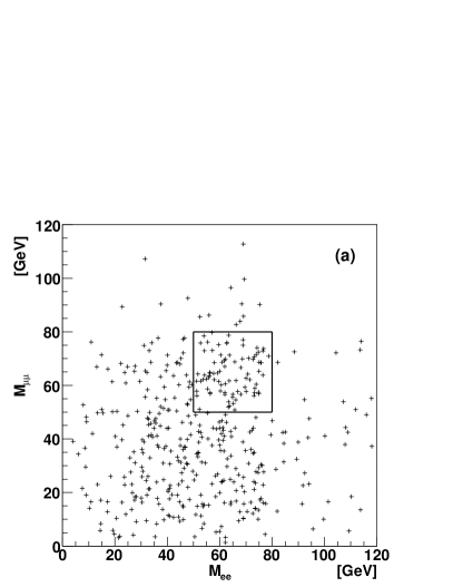
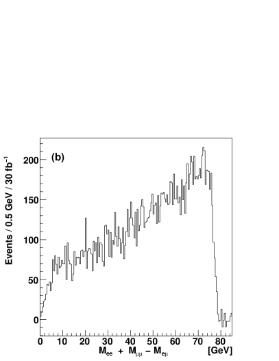
Figure 4: (a) Wedgebox plot for 300 fb^-1 of integrated LHC luminosity at the SPS1a benchmark point. Events are sampled from the boxed region shown for DK analysis. (b) The flavor-subtracted dilepton invariant mass distribution provides a clean determination of the edge $M_{\ell\ell}^{max}=77.1$ GeV. The plot is shown for an integrated luminosity of 30 fb^-1.

Events in a broad neighborhood of the corner of the box, $M_{ee,\mu\mu}=65\pm\epsilon$ GeV (see further comments below on sampling regions), are passed to the on-shell DK analysis described in the previous Section. In detail, the procedure used is the following:

1. An event is selected if the two invariant masses $M_{ee}$ and $M_{\mu\mu}$ both lie within the $\epsilon$-defined region of the wedgebox plot.

2. A point in $(\hbox to0.0pt{\hbox to7.80904pt{\hfil/\hfil}\hss}P_{Tx},~{}\hbox to0.0pt{\hbox to7.80904pt{\hfil/\hfil}\hss}P_{Ty})$-space is chosen by a uniform scan of $-500$ GeV $<\hbox to0.0pt{\hbox to7.80904pt{\hfil/\hfil}\hss}P_{Tx,y}<$ $500$ GeV, in $0.2$ GeV steps; the point is assumed to equal the transverse momentum of the LSP accompanying the $e^{+}$ and $e^{-}$ whose four-momenta are $(E,\vec{P})_{1,2}$, respectively.

3. The longitudinal component of the LSP’s momentum is found from (22).

4. Components of the LSP momentum in the basis parallel/perpendicular to the total leptonic momentum $\vec{P}=\vec{P}_{1}+\vec{P}_{2}$ are determined and used to compute $\alpha\equiv\hbox to0.0pt{\hbox to7.80904pt{\hfil/\hfil}\hss}P_{\bot}/(\hbox to0.0pt{\hbox to7.80904pt{\hfil/\hfil}\hss}P_{\|}+P)$.

5. The boost parameters $\beta_{\|}$ and $\beta_{\bot}$ are now computed from (21), $K^{\|}$ and $K^{\bot}$ from (23).

6. The masses $\{m_{1}^{\prime},~{}m_{2}^{\prime}\}$ are computed from (24) and (25).

7. Using the missing momentum constraint $\vec{p}_{\chi^{\prime}}^{~{}T}=\not\!\vec{p}^{~{}T}-\vec{p}_{\chi}^{~{}T}$, steps 3-6 are repeated for the LSP accompanying the $\mu^{+}\mu^{-}$ pair, obtaining either another set of masses $\{m_{1}^{\prime\prime},~{}m_{2}^{\prime\prime}\}$ or no valid solution for the second mass set.

8. If no valid second set of masses was obtained, the point is assigned zero weight. Otherwise, the two sets of mass solutions are plotted with the following weight:

   $$P(\hbox to0.0pt{\hbox to7.80904pt{\hfil/\hfil}\hss}P_{Tx},\hbox to0.0pt{\hbox to7.80904pt{\hfil/\hfil}\hss}P_{Ty})=\frac{1}{\sqrt{2\pi\sigma^{2}}}\exp\left(-\frac{(m_{1}^{\prime}-m_{1}^{\prime\prime})^{2}}{2\sigma^{2}}-\frac{(m_{2}^{\prime}-m_{2}^{\prime\prime})^{2}}{2\sigma^{2}}\right),$$ (26)

   where $\sigma$ is our expectation for the spread between the mass values on either side of the event. This should be of the order of the missing energy resolution, which is a function of the total transverse energy $E_{T}$ deposited in the calorimeters. We therefore assign sigma on an event-by-event basis, using the expected performance of the ATLAS detector in SUSY events (see figure 10.84 of reference  [31]):

   $$\sigma=0.57\sqrt{\sum E_{T}}.$$ (27)

9. The scan is continued until all points have been assigned a weight.

10. The procedure is repeated for all events that have invariant masses sufficiently close to the endpoint.

Our final mass distribution for a single event is obtained by histogramming all mass solutions found in the scan over missing momentum components, weighted by Eq. (26). For events that lie exactly at the endpoint, and where the mismeasurement of lepton momenta and missing energy is negligible, the peak of the two mass distributions for $\{m_{1}^{\prime},~{}m_{2}^{\prime}\}$ and $\{m_{1}^{\prime\prime},~{}m_{2}^{\prime\prime}\}$ should coincide, agreeing with the nominal values of the masses. We find that this remains accurate for events that lie sufficiently close to the endpoint, and thus with a value of $\epsilon$ that is not too large.

In fact, choosing a value of $\epsilon$ is essentially a trade-off between accumulating statistics by allowing more events to pass the cut, thus reducing the fluctuations that come from the smearing of lepton and missing energy momenta, and protecting the integrity of the mass solutions that are obtained by the procedure at $\epsilon=0$. We find that a compromise value for $\epsilon$ of 15 GeV gives just enough events with peak region close to the nominal values to dominate over events that display either one or two degenerate peaks or peaks in the wrong place. In the latter case, we observe that the maximum weight at the peak is lower.

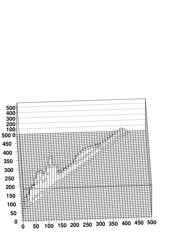
Figure 5: Mass distribution for 300 fb^-1 of data at SPS1a, obtained using the procedure described in the text. The contribution of individual events with degenerate solutions is still clearly visible, although it is a region close to the nominal mass values of $(m_{1},m_{2})=(96.1,176.8)$ GeV that emerges with the largest total weight.

By summing the distributions for events within our choice of $\epsilon$, the resulting total mass distribution for 300 fb^-1 of data is shown in Fig. 5. Although the existence of multiple peaks is clear with the limited statistics, the point with the largest total weight is found to be $(m_{1},m_{2})=(114.75,191.75)$ GeV, close to the nominal value of $(m_{1},m_{2})=(96.1,176.8)$ GeV. We emphasize that this procedure is simply a suggestion for an estimator of the masses, and although there are similarities in shape, Eq. (26) is not a likelihood function.

To check the robustness of the estimator and find the statistical error on making such a measurement, we have performed 10 independent ‘experiments’ with 300 fb^-1 integrated luminosity. In each case, the mass solution with the largest total weight fell near the nominal masses, with a standard deviation of 20.2 GeV on $m_{1}$ and 21.2 GeV on $m_{2}$. While these errors are quite large, there is undoubtedly scope for improvement. By better understanding the properties of events with degenerate or wrong solutions one could search for a system of kinematic cuts to remove these subsets; one could also increase statistics to tighten the cut on $\epsilon$ or investigate other estimators for the masses with better properties with respect to these events.

Incidentally, had we wrongly assumed off-shell kinematics at this parameter point, and hence tried using the technique of Section 2 to analyze events in the boxed region of Fig. 4a, we would have failed since essentially no events provide two mass solutions with a near equal mass. This provides a way of distinguishing a sample of on- versus off-shell decays distinct from the usual way of measuring the departure of the di-lepton mass distribution from a triangular shape [19], or looking for specific relationships between the positions of lepton-jet invariant mass maxima [41].

Finally, note that this method, although we have not explicitly demonstrated it, is in principle also applicable to extracting the slepton mass.

4 Conclusions

This paper completes the demonstration of the application of the DK technique to neutralino decays in SUSY models, or indeed any similar decay chain in models such as e.g. UED [42], having explicitly shown the procedure for reconstructing both off- and on-shell decays to lepton pairs in realistic MC simulations of two very different supersymmetry benchmark points. We find that in the three-body decay scenario we can reconstruct the LSP mass with an accuracy of around 4 GeV, while the decay through an on-shell slepton allows a precision of 20 GeV.

DK has the advantage of simplicity and robustness in the face of backgrounds; for non-signal events there tends to be no solution for the constraint equations, or at least no preferred solution in the distribution of events passing loose constraint requirements. Moreover, since the method only makes use of unlike di-leptons ($e^{+}e^{-}\mu^{+}\mu^{-}$) from the $\tilde{\chi}^{0}_{2}\to\tilde{\chi}^{0}_{1}$ transitions, it is insensitive to the combinatoric issues that arise when one considers particles produced further up the decay chain. It may hence complement mass determinations which exploit the full chains such as [5, 6]. Generalization to other decaying states (e.g. charginos as in [43]), perhaps using jets instead of or in addition to leptons, is open to investigation.

Perhaps the major disadvantage of DK is the requirement of a high event rate: one typically needs at least ${\mathcal{O}}(10)$ events in the neighborhood of a kinematic endpoint to make the reconstruction stable, and, in the case of four-lepton final states, that translates to several hundreds of events needed on a wedgebox plot. In addition, the case of on-shell decays gives rise to extra solutions in the mass space that can be eliminated with more statistics, but ultimately contribute to an increased error in the reconstructed masses.

Thus, in the case of neutralino-pair production considered in this work, DK may, depending on the parameter point Nature has chosen, perhaps only serve useful as a check on results obtained with other techniques that do not depend on events near an endpoint. As mentioned in the Introduction, these most prominently include MSTs and $m_{T2}$ techniques, which at the SPS1a point happen to work quite well.

Appendix

On-Shell Kinematics

Consider the neutralino decay

$$\tilde{\chi}_{i}^{0}\to\ell^{+}\tilde{\ell}^{-}\to\ell^{+}\ell^{-}\tilde{\chi}_{1}^{0},$$ (28)

in the neutralino rest frame. If the di-lepton invariant mass is maximal, all the decay products must be collinear (say along $\hat{x}$). In particular, four-momentum conservation forces

$$\left(\begin{array}[]{c}E_{\ell^{+}}\\ \\ p_{\ell^{+}}\\ \end{array}\right)_{\tilde{\chi}_{i}^{0}}=\left(\begin{array}[]{c}\frac{m_{i}^{2}-m_{s}^{2}}{2m_{i}}\\ \\ \frac{m_{i}^{2}-m_{s}^{2}}{2m_{i}}\\ \end{array}\right)\quad{\rm and}\quad\left(\begin{array}[]{c}E_{\tilde{\ell}^{-}}\\ \\ p_{\tilde{\ell}^{-}}\\ \end{array}\right)_{\tilde{\chi}_{i}^{0}}=\left(\begin{array}[]{c}\frac{m_{i}^{2}+m_{s}^{2}}{2m_{i}}\\ \\ -\frac{m_{i}^{2}-m_{s}^{2}}{2m_{i}}\\ \end{array}\right),$$

where $m_{s}$ is the slepton mass and the lepton is assumed to be massless. Similarly, in the slepton’s decay frame,

$$\left(\begin{array}[]{c}E_{\ell^{-}}\\ \\ p_{\ell^{-}}\\ \end{array}\right)_{\tilde{\ell}}=\left(\begin{array}[]{c}\frac{m_{s}^{2}-m_{1}^{2}}{2m_{s}}\\ \\ -\frac{m_{s}^{2}-m_{1}^{2}}{2m_{s}}\\ \end{array}\right)\quad{\rm and}\quad\left(\begin{array}[]{c}E_{\tilde{\chi}_{1}^{0}}\\ \\ p_{\tilde{\chi}_{1}^{0}}\\ \end{array}\right)_{\tilde{\ell}}=\left(\begin{array}[]{c}\frac{m_{s}^{2}+m_{1}^{2}}{2m_{s}}\\ \\ \frac{m_{s}^{2}-m_{1}^{2}}{2m_{s}}\\ \end{array}\right),$$

which, when boosted back to the $\tilde{\chi}_{i}^{0}$ rest frame using $\beta=-(m_{i}^{2}-m_{s}^{2})/(m_{i}^{2}+m_{s}^{2})$, becomes

$$\left(\begin{array}[]{c}E_{\ell^{-}}\\ \\ p_{\ell^{-}}\\ \end{array}\right)_{\tilde{\chi}_{i}^{0}}=\left(\begin{array}[]{c}m_{i}\frac{m_{s}^{2}-m_{1}^{2}}{2m_{s}^{2}}\\ \\ -m_{i}\frac{m_{s}^{2}-m_{1}^{2}}{2m_{s}^{2}}\\ \end{array}\right)\quad{\rm and}\quad\left(\begin{array}[]{c}E_{\tilde{\chi}_{1}^{0}}\\ \\ p_{\tilde{\chi}_{1}^{0}}\\ \end{array}\right)_{\tilde{\chi}_{i}^{0}}=\left(\begin{array}[]{c}\frac{m_{s}^{4}+m_{i}^{2}m_{1}^{2}}{2m_{i}m_{s}^{2}}\\ \\ \frac{m_{s}^{4}-m_{i}^{2}m_{1}^{2}}{2m_{i}m_{s}^{2}}\\ \end{array}\right).$$

From these equations it is easy to verify (10), (11), (14), and (15).

Finding the Lorentz Boost Parameters

Here we indicate in more detail how one may arrive at Eq. (21). Starting from Eq. (20) we have two relevant equations,

$$\hbox to0.0pt{\hbox to7.80904pt{\hfil/\hfil}\hss}P_{\|}+K_{i}^{\|} = \beta_{\|}\left(\gamma\sqrt{K_{i}^{2}+m_{1}^{2}}-(\gamma-1)\frac{\beta_{\|}}{\beta^{2}}K_{i}^{\|}-(\gamma-1)\frac{\beta_{\bot}}{\beta^{2}}K_{i}^{\bot}\right),$$

$$\hbox to0.0pt{\hbox to7.80904pt{\hfil/\hfil}\hss}P_{\bot}+K_{i}^{\bot} = \beta_{\bot}\left(\gamma\sqrt{K_{i}^{2}+m_{1}^{2}}-(\gamma-1)\frac{\beta_{\|}}{\beta^{2}}K_{i}^{\|}-(\gamma-1)\frac{\beta_{\bot}}{\beta^{2}}K_{i}^{\bot}\right).$$

Taking the ratio of these one obtains after some rearranging

$$K_{i}^{\|}=\frac{\beta_{\|}}{\beta_{\bot}}\hbox to0.0pt{\hbox to7.80904pt{\hfil/\hfil}\hss}P_{\bot}+\frac{\beta_{\|}}{\beta_{\bot}}K_{i}^{\bot}-\hbox to0.0pt{\hbox to7.80904pt{\hfil/\hfil}\hss}P_{\|}.$$ (29)

This can now be inserted into two of the equations of (19),

$$K_{i}^{\|} = -\beta_{\|}\gamma E+P+P(\gamma-1)\frac{\beta_{\|}^{2}}{\beta^{2}},$$ (30)

$$K_{i}^{\bot} = -\beta_{\bot}\gamma E+(\gamma-1)\frac{\beta_{\|}\beta_{\bot}}{\beta^{2}}P,$$ (31)

which can then be used to solve for the ratio

$$\alpha\equiv\frac{\beta_{\bot}}{\beta_{\|}}=\frac{\hbox to0.0pt{\hbox to7.80904pt{\hfil/\hfil}\hss}P_{\bot}}{P+\hbox to0.0pt{\hbox to7.80904pt{\hfil/\hfil}\hss}P_{\|}}.$$ (32)

Starting from the antiparallel condition (17) and expanding with the lepton momenta from (18), one arrives, after some algebra, at

$$0=(1+\beta_{\|}^{2}+\beta_{\bot}^{2})E_{1}E_{2}-2\beta_{\|}E_{1}P_{2}^{\|}-2\beta_{\bot}E_{1}P_{2}^{\bot}-2\beta_{\|}E_{2}P_{1}^{\|}-2\beta_{\bot}E_{2}P_{1}^{\bot}+$$

$$2\beta_{\|}\beta_{\bot}(P_{1}^{\|}P_{2}^{\bot}+P_{2}^{\|}P_{1}^{\bot})+(1+\beta_{\|}^{2}-\beta_{\bot}^{2})P_{1}^{\|}P_{2}^{\|}+(1-\beta_{\|}^{2}+\beta_{\bot}^{2})P_{1}^{\bot}P_{2}^{\bot},$$

using that $E_{1,2}=|\vec{P}_{1,2}|$. Substituting $\beta_{\bot}$ for $\alpha$ and $\beta_{\|}$ from (32), we get a quadratic equation for $\beta_{\|}$:

$$0=a\beta_{\|}^{2}-2b\beta_{\|}+c,$$

where

$$a \equiv E_{1}E_{2}+P_{1}^{\|}P_{2}^{\|}-P_{1}^{\bot}P_{2}^{\bot}+2\alpha(P_{1}^{\|}P_{2}^{\bot}+P_{2}^{\|}P_{1}^{\bot})+\alpha^{2}(E_{1}E_{2}-P_{1}^{\|}P_{2}^{\|}+P_{1}^{\bot}P_{2}^{\bot}),$$

$$b \equiv E_{1}P_{2}^{\|}+E_{2}P_{1}^{\|}+\alpha(E_{1}P_{2}^{\bot}+E_{2}P_{1}^{\bot}),$$

$$c \equiv E_{1}E_{2}+P_{1}^{\|}P_{2}^{\|}+P_{1}^{\bot}P_{2}^{\bot}.$$

Using again that $E_{1,2}^{2}={P_{1,2}^{\|}}^{2}+{P_{1,2}^{\bot}}^{2}$, one can show that $b^{2}-4ac=0$, so this quadratic has a double root

$$\beta_{\|}=\frac{E_{1}P_{2}^{\|}+E_{2}P_{1}^{\|}+\alpha(E_{1}P_{2}^{\bot}+E_{2}P_{1}^{\bot})}{E_{1}E_{2}+P_{1}^{\|}P_{2}^{\|}-P_{1}^{\bot}P_{2}^{\bot}+2\alpha(P_{1}^{\|}P_{2}^{\bot}+P_{1}^{\bot}P_{2}^{\|})+\alpha^{2}(E_{1}E_{2}-P_{1}^{\|}P_{2}^{\|}+P_{1}^{\bot}P_{2}^{\bot})}.$$

Making repeated use of that, by definition, $P_{1}^{\bot}=-P_{2}^{\bot}$ and $P=P_{1}^{\|}+P_{2}^{\|}$, one arrives at the equation for $\beta_{\|}$ in (21).

References

- [1] K. Kawagoe, M. M. Nojiri and G. Polesello, Phys. Rev. D71, 035008 (2005), [hep-ph/0410160].
- [2] M. M. Nojiri, G. Polesello and D. R. Tovey, JHEP 05, 014 (2008), [0712.2718].
- [3] H.-C. Cheng, J. F. Gunion, Z. Han, G. Marandella and B. McElrath, JHEP 12, 076 (2007), [0707.0030].
- [4] H.-C. Cheng, D. Engelhardt, J. F. Gunion, Z. Han and B. McElrath, Phys. Rev. Lett. 100, 252001 (2008), [0802.4290].
- [5] H.-C. Cheng, J. F. Gunion, Z. Han and B. McElrath, 0905.1344.
- [6] B. Webber, 0907.5307.
- [7] M. Bisset, R. Lu and N. Kersting, 0806.2492.
- [8] C. G. Lester and D. J. Summers, Phys. Lett. B463, 99 (1999), [hep-ph/9906349].
- [9] A. Barr, C. Lester and P. Stephens, J. Phys. G29, 2343 (2003), [hep-ph/0304226].
- [10] W. S. Cho, K. Choi, Y. G. Kim and C. B. Park, Phys. Rev. Lett. 100, 171801 (2008), [0709.0288].
- [11] A. J. Barr, B. Gripaios and C. G. Lester, JHEP 02, 014 (2008), [0711.4008].
- [12] W. S. Cho, K. Choi, Y. G. Kim and C. B. Park, JHEP 02, 035 (2008), [0711.4526].
- [13] M. M. Nojiri, Y. Shimizu, S. Okada and K. Kawagoe, JHEP 06, 035 (2008), [0802.2412].
- [14] A. J. Barr, G. G. Ross and M. Serna, Phys. Rev. D78, 056006 (2008), [0806.3224].
- [15] D. J. Miller, P. Osland and A. R. Raklev, JHEP 03, 034 (2006), [hep-ph/0510356].
- [16] S. Kraml and A. R. Raklev, Phys. Rev. D73, 075002 (2006), [hep-ph/0512284].
- [17] B. K. Gjelsten, D. J. Miller, P. Osland and A. R. Raklev, hep-ph/0611080.
- [18] B. K. Gjelsten, D. J. Miller, P. Osland and A. R. Raklev, AIP Conf. Proc. 903, 257 (2007), [hep-ph/0611259].
- [19] S. Kraml, A. R. Raklev and M. J. White, Phys. Lett. B672, 361 (2009), [0811.0011].
- [20] I. Hinchliffe, F. E. Paige, M. D. Shapiro, J. Soderqvist and W. Yao, Phys. Rev. D55, 5520 (1997), [hep-ph/9610544].
- [21] F. E. Paige, hep-ph/9801254.
- [22] H. Bachacou, I. Hinchliffe and F. E. Paige, Phys. Rev. D62, 015009 (2000), [hep-ph/9907518].
- [23] E. Lytken, ATL-PHYS-2004-001.
- [24] B. K. Gjelsten, D. J. Miller and P. Osland, JHEP 12, 003 (2004), [hep-ph/0410303].
- [25] B. K. Gjelsten, D. J. Miller and P. Osland, JHEP 06, 015 (2005), [hep-ph/0501033].
- [26] P. Huang, N. Kersting and H. H. Yang, Phys. Rev. D77, 075011 (2008), [0801.0041].
- [27] M. Burns, K. T. Matchev and M. Park, JHEP 05, 094 (2009), [0903.4371].
- [28] K. T. Matchev, F. Moortgat, L. Pape and M. Park, 0906.2417.
- [29] N. Kersting, Phys. Rev. D79, 095018 (2009), [0901.2765].
- [30] B. C. Allanach et al., Eur. Phys. J. C25, 113 (2002), [hep-ph/0202233].
- [31] ATLAS Collaboration, G. Aad et al., JINST 3, S08003 (2008).
- [32] T. Sjostrand, S. Mrenna and P. Skands, JHEP 05, 026 (2006), [hep-ph/0603175].
- [33] G. Corcella et al., JHEP 01, 010 (2001), [hep-ph/0011363].
- [34] S. Moretti, K. Odagiri, P. Richardson, M. H. Seymour and B. R. Webber, JHEP 04, 028 (2002), [hep-ph/0204123].
- [35] M. L. Mangano, M. Moretti, F. Piccinini, R. Pittau and A. D. Polosa, JHEP 07, 001 (2003), [hep-ph/0206293].
- [36] J. M. Butterworth, J. R. Forshaw and M. H. Seymour, Z. Phys. C72, 637 (1996), [hep-ph/9601371].
- [37] E. Richter-Was, hep-ph/0207355.
- [38] M. Bisset et al., Eur. Phys. J. C45, 477 (2006), [hep-ph/0501157].
- [39] ATLAS Collaboration, I. Hinchliffe et al., CERN-LHCC-99-15.
- [40] ATLAS Collaboration, G. Aad et al., 0901.0512.
- [41] C. G. Lester, M. A. Parker and M. J. White, JHEP 10, 051 (2007), [hep-ph/0609298].
- [42] T. Appelquist, H.-C. Cheng and B. A. Dobrescu, Phys. Rev. D64, 035002 (2001), [hep-ph/0012100].
- [43] N. Kersting, Eur. Phys. J. (in press) , [0806.4238].