Symmetric sequence processing in a recurrent neural network model with a synchronous dynamics

Abstract

The synchronous dynamics and the stationary states of a recurrent attractor neural network model with competing synapses between symmetric sequence processing and Hebbian pattern reconstruction is studied in this work allowing for the presence of a self-interaction for each unit. Phase diagrams of stationary states are obtained exhibiting phases of retrieval, symmetric and period-two cyclic states as well as correlated and frozen-in states, in the absence of noise. The frozen-in states are destabilised by synaptic noise and well separated regions of correlated and cyclic states are obtained. Excitatory or inhibitory self-interactions yield enlarged phases of fixed-point or cyclic behaviour.

1 Introduction

The asymptotic stationary states of large recurrent attractor neural network models trained with sequences of patterns have been studied some time ago [1]-[10] and there has been a recent revival of interest near the storage saturation of patterns [11]-[17]. Besides network models for asymmetric sequence processing, models with synapses generated by symmetric sequences competing with pattern reconstruction favoured by Hebbian synapses have been studied in some of those works [3, 4, 8, 16]. These are models with an underlying asynchronous dynamics and phase diagrams were obtained which only exhibit fixed-point solutions, in particular correlated attractors, in accordance with a general expectation for networks with symmetric interaction matrices far from the storage saturation limit in which the ratio $\alpha=p/N$ of the number of stored patterns $p$ and the number of neurons $N$ is zero, in the large $N$ limit. In contrast, in the case of a synchronous dynamics with symmetric interactions the stationary states may be either fixed-points or cycles of period two, in the same limit [18]. Rhythmic activity appears in neurobiological systems [19] and the competition between these features may yield interesting clues.

The presence of self-interactions of the units, which is consistent with detailed balance in the synchronous dynamics of a network with a symmetric interaction matrix, has not been considered so far except in Little’s model which has a simple Hebbian learning rule [20]-[25]. The role of self-interactions which may be either excitatory or inhibitory, is to control the fraction of spin flips in the dynamics. Excitatory interactions may enhance the retrieval performance while inhibitory interactions can give rise to cyclic behaviour. Self-interactions and their relationship to initial overlaps play a crucial role in Little’s model leading to frozen-in cycles of period two among other features, in the absence of noise [21, 22]. In a recent work it has been shown that these cycles are destabilised in a slow dynamical process either by synaptic or stochastic noise due to a macroscopic number of stored patterns [25]. This raises concern about the stability of cycles of period two in general in the synchronous dynamics of networks with symmetric interactions for the specific interesting case of symmetric sequence processing competing with Hebbian synapses.

There has been great interest in models with symmetric sequential interactions due to the presence of correlated fixed-point attractors [4, 8, 16, 29], which are stationary states that emerge from a balanced competition between sequential and Hebbian synapses. They indicate a selectivity in response to a set of previously learned uncorrelated patterns by means of decreasing correlation coefficients for the attractors with increasingly distant patterns from a stimulus. Correlated attractors have been used to explain the results of experimental recordings of a visual-memory task in the inferotemporal cortex of monkeys [26]-[29]. In the case of a synchronous dynamics, the correlated fixed-point states might be destabilised by the presence of a macroscopic number of flipping spins giving rise to oscillatory overlaps.

The asymptotic states of a feed-forward layered neural network model for competing symmetric sequence processing with Hebbian synapses have been discussed in a recent work [30]. The model is described by a synchronous dynamics and it is characterised by asymmetric synaptic connections between units in two consecutive layers and there are neither lateral synapses between units in the same layer nor self-interactions of the units. Phase diagrams of stationary states were obtained exhibiting retrieval states, correlated states, symmetric mixture states and stable cycles of period two, for increasingly larger fractions of sequential synapses. All of these states are robust either to synaptic noise or to stochastic noise due to a macroscopic number of stored patterns.

The purpose of the present paper is to study the synchronous dynamics and the asymptotic states of a recurrent network model of binary units and patterns for competing interaction between symmetric sequence processing and Hebbian synapses, in order to investigate the presence and stability of cycles of period two and of other states which could be competing with the retrieval and with the correlated states. We make use of a generating functional approach (GFA) for the dynamics of disordered systems [11, 31], which is an exact procedure in the mean-field limit, and we use an adaptation of the numerical simulation procedure of Eissfeller and Opper (EO) [32] based on the GFA in order to implement the calculation of single-site averages. We also resort to a recently introduced alternative approach [25].

The outline of the paper is the following. We introduce the model in section 2 and present a brief summary of the well known GFA and the EO procedure in section 3 as well as explicit dynamic recursion relations for the overlaps. We present our results for the phase diagrams in section 4 and conclude with a summary and further discussion in section 5.

2 The model

We consider a network of $N$ Ising neurons in a microscopic state $\mbox{\boldmath$\sigma$}^{t}=(\sigma_{1}^{t},\dots,\sigma_{N}^{t})$, at the discrete time-step $t$ in which each $\sigma_{i}^{t}=\pm 1$ represents the state of an active or inactive neuron, respectively. The states of all neurons are updated simultaneously at each time-step according to the alignment of each spin with its local field

$$h_{i}^{t}=\sum_{j}J_{ij}\sigma_{j}^{t}+\theta_{i}^{t}\,\,\,,$$ (1)

following a microscopic stochastic single spin-flip dynamics with transition probability

$$w(\sigma_{i}^{t+1}|h_{i}^{t})=\frac{1}{2}\big{[}1+\sigma_{i}^{t+1}\tanh{(\beta h_{i}^{t})}\big{]}\,\,\,$$ (2)

ruled by the synaptic noise control parameter $\beta=T^{-1}$. Here, $J_{ij}$ is the synaptic coupling between neurons $i$ and $j$ and $\theta_{i}^{t}$ is an external stimulus. The dynamics is a deterministic one when $T=0$ and fully random when $T=\infty$. In the former case, $\sigma_{i}^{t+1}={\rm sgn}(h_{i}^{t})$.

A macroscopic set $\mbox{\boldmath$\xi$}^{\mu}=(\xi_{1}^{\mu},\dots,\xi_{N}^{\mu})$, $\mu=1,\dots,p$ of $p=\alpha N$ independent and identically distributed quenched random patterns, each $\xi_{i}^{\mu}=\pm 1$ with probability $\frac{1}{2}$, is embedded in the network by means of the synaptic coupling $J_{ij}$ between distinct neurons $i$ and $j$. One may think of $j$ and $i$ as pre- and post-synaptic neurons, respectively, the activities of which give rise to that coupling. We assume, as usual, that a finite number $c$ of patterns is condensed so that the overlaps with the state of the network, defined below, are finite and responsible for the signal in the local field. The remaining macroscopic number of $p-c$ non-condensed patterns will give rise to the noise in the local field. To be specific, we assume that the condensed patterns are cyclic so that $\mbox{\boldmath$\xi$}^{c+1}=\mbox{\boldmath$\xi$}^{1}$.

The non-condensed patterns need not be embedded in the network by the same learning rule as that for the condensed patterns. Indeed, one may think that those patterns have been learned in a previous stage, in accordance with an argument that has been used before [4]. We make use of this freedom in order to simplify the calculations by assuming a Hebbian rule for the non-condensed patterns. Guided by work on the layered feed-forward network [30], we expect qualitatively the same results as those obtained here for the same learning rule for condensed and non-condensed patterns. Thus, altogether, we take a synaptic coupling of the form

$$J_{ij} =\frac{\nu}{N}\sum_{\mu=1}^{c}\xi_{i}^{\mu}\xi_{j}^{\mu}+\frac{1-\nu}{N}\sum_{\mu=1}^{c}(\xi_{i}^{\mu}\xi_{j}^{\mu+1}+\xi_{i}^{\mu+1}\xi_{j}^{\mu})+\frac{1}{N}\sum_{\mu=c+1}^{p}\xi_{i}^{\mu}\xi_{j}^{\mu}\,\,\,\,\,\,\,{\rm if}\,\,\,\,\,i\neq j\,\,\,$$ (3)

$$=J_{0}\,\,\,\,\,\,\,\,{\rm if}\,\,\,\,\,i=j\,\,\,,$$

in which each value of $\nu$ $(0\leq\nu\leq 1)$ defines a model so that when $\nu=1$ we get Little’s model with a Hebbian rule and when $\nu=0$ we have the purely symmetric sequential model. The first and the second summations are responsible for the signal in the local field while the last summation is responsible for the noise and we comment on that term in section 5. The self-interaction $J_{0}$ is a real non-random variable which can take any positive or negative value enhancing or inhibiting, respectively, the local field in the form of a pattern-independent contribution $J_{0}\sigma_{i}^{t}$. It either tends to enforce the actual state of unit $i$, if $J_{0}$ is positive, or to switch the state if $J_{0}$ is negative.

3 The dynamic generating functional approach

The dynamical evolution of the system is described by the moment generating functional [11]

$$Z(\mbox{\boldmath$\psi$}) =\Big{\langle}\exp\Big{(}-\rmi\sum_{i}\sum_{s=0}^{t}\psi_{i}^{s}\,\sigma_{i}^{s}\Big{)}\Big{\rangle}$$ (4)

$$=\sum_{\mbox{\boldmath$\sigma$}^{0},\dots,\mbox{\boldmath$\sigma$}^{t}}\mathrm{Prob}(\mbox{\boldmath$\sigma$}^{0},\dots,\mbox{\boldmath$\sigma$}^{t})\exp\Big{(}-\rmi\sum_{i}\sum_{s=0}^{t}\psi_{i}^{s}\,\sigma_{i}^{s}\Big{)}\,\,,$$

where $\mbox{\boldmath$\psi$}^{s}=(\psi_{1}^{s},\dots,\psi_{N}^{s})$ is a set of auxiliary variables that serve to generate averages of moments of the states and the brackets denote an average over all possible paths of states with probability

$$\mathrm{Prob}(\mbox{\boldmath$\sigma$}^{0},\dots,\mbox{\boldmath$\sigma$}^{t})=p(\mbox{\boldmath$\sigma$}^{0})\prod_{s=0}^{t-1}\prod_{i}\frac{\exp(\,\beta\,\sigma_{i}^{s+1}\,h_{i}^{s})}{2\,\mathrm{cosh}(\beta\,h_{i}^{s})}$$ (5)

that follows from (2). Assuming that for $N\rightarrow\infty$ only the statistical properties of the stored patterns will influence the macroscopic behaviour of the system, one obtains the relevant quantities which are the overlap $m^{t}_{\mu}$ of $O(1)$ with any one of the condensed patterns $\mbox{\boldmath$\xi$}^{\mu}$, the two-time correlation function $C_{tl}$ and the response function $G_{tl}$, given by

$$m_{\mu}^{t}=\frac{1}{N}\sum_{i}\overline{\xi_{i}^{\mu}\langle\sigma_{i}^{t}\rangle}=\lim_{\mbox{\boldmath$\psi$}\rightarrow 0}\frac{\rmi}{N}\sum_{i}\xi_{i}^{\mu}\frac{\partial\overline{Z(\mbox{\boldmath$\psi$})}}{\partial\psi_{i}^{t}}\,\,,$$ (6)

$$C_{tl}=\frac{1}{N}\sum_{i}\overline{\langle\sigma_{i}^{t}\sigma_{i}^{l}\rangle}=-\lim_{\mbox{\boldmath$\psi$}\rightarrow 0}\frac{1}{N}\sum_{i}\frac{\partial^{2}\overline{Z(\mbox{\boldmath$\psi$})}}{\partial\psi_{i}^{l}\psi_{i}^{t}}\,\,$$

and

$$G_{tl}=\frac{1}{N}\sum_{i}\frac{\partial\overline{\langle\sigma_{i}^{t}\rangle}}{\partial\theta_{i}^{l}}=\rmi\,\lim_{\mbox{\boldmath$\psi$}\rightarrow 0}\frac{1}{N}\sum_{i}\frac{\partial^{2}\overline{Z(\mbox{\boldmath$\psi$})}}{\partial\theta_{i}^{l}\psi_{i}^{t}}\,\,\,\,(l<t)\,\,,$$ (7)

where the bar denotes the configurational average with the non-condensed patters $\{\mbox{\boldmath$\xi$}^{\rho}\}$ ($\rho=c+1,\dots,p$) and the restriction $l<t$ is due to causality. The two-consecutive-time correlation function has a particular meaning since $q_{t}=C_{t,t-1}$ gives the fraction of flipping spins between two consecutive times as $(1-q_{t})/2$.

Following the now standard procedure in which the disorder average is done before the sum over the neuron states one obtains exactly, in the large $N$ limit, the generating functional [11, 32]

$$\overline{Z(\mbox{\boldmath$\psi$})}=\Big{\langle}\sum_{\mbox{\boldmath$\sigma$}^{0},\dots,\mbox{\boldmath$\sigma$}^{t}}p(\mbox{\boldmath$\sigma$}^{0})\exp\Big{(}-i\sum_{i}\sum_{s=0}^{t}\psi_{i}^{s}\,\sigma_{i}^{s}\Big{)}$$

$$\prod_{i}\prod_{s<t}\Big{[}\int dh_{i}^{s}\,\delta(h_{i}^{s}-h_{\mathrm{eff}}^{s})\,\mathrm{w}(\sigma_{i}^{s+1}|h_{i}^{s})\Big{]}\Big{\rangle}_{\{\phi_{i}^{s}\}}$$ (8)

in which $p(\mbox{\boldmath$\sigma$}^{0})=\prod_{i}p(\sigma_{i}^{0})$ is the probability of the initial microscopic configuration while $\langle\dots\rangle_{\{\phi_{i}^{t}\}}$ denotes an average over a set of temporarily correlated Gaussian random variables $\{\phi_{i}^{t}\}$ for unit $i$, with zero-average and a correlation matrix given below. The random variables on different units turn out to be uncorrelated and one is left with a single-site effective theory in which a neuron evolves in time according to the transition probability

$$\mathrm{w}(\sigma^{t+1}|h_{\mathrm{eff}}^{t})=\frac{1}{2}\Big{[}1+\sigma^{t+1}\tanh{\big{(}\beta h_{\mathrm{eff}}^{t}\big{)}}\Big{]}\,\,$$ (9)

with an effective local field given by

$$h_{\mathrm{eff}}^{t}=\sum_{\mu,\rho\leq c}\xi^{\mu}A_{\mu\rho}m^{t}_{\rho}+J_{0}\sigma^{t}+\alpha\sum_{s<t}R_{ts}\sigma^{s}+\sqrt{\alpha}\phi^{t}\,\,,$$ (10)

where

$$A_{\mu\rho}=\nu\delta_{\mu,\,\rho}+(1-\nu)\,(\delta_{\mu,\,\rho+1}+\delta_{\mu,\,\rho-1})\,\,,$$ (11)

and we assumed that $\theta^{t}=0$. The two non-trivial contributions to the effective local field for $\alpha>0$ come from a retarded self-interaction involving the matrix elements

$$R_{ts}=[\mbox{\boldmath$G$}(\mbox{\boldmath$I$}-\mbox{\boldmath$G$})^{-1}]_{ts}$$ (12)

and the zero-average temporarily correlated Gaussian noise $\phi^{t}$ with variance

$$S_{ts}=\langle\phi^{t}\phi^{s}\rangle_{\{\phi^{t}\}}=[(\mbox{\boldmath$I$}-\mbox{\boldmath$G$})^{-1}\mbox{\boldmath$C$}(\mbox{\boldmath$I$}-\mbox{\boldmath$G$}^{\dagger})^{-1}]_{ts}\,\,.\\$$ (13)

Here, $C$ and $G$ are matrices with elements $\{C_{ts}\}$ and $\{G_{ts}\}$, respectively. Both contributions account for memory effects in the network that come from the noise in the original local field due to the macroscopically large number of non-condensed patterns.

The dynamics of each of the macroscopic quantities, given by (6-7), is obtained from the statistics of the effective single neuron process through the average

$$\langle f(\mbox{\boldmath$\sigma$})\rangle_{*}=\int d\mbox{\boldmath$\phi$}\mathrm{P}(\mbox{\boldmath$\phi$})\sum_{\mbox{\boldmath$\sigma$}}\mathrm{P}(\mbox{\boldmath$\sigma$}|\mbox{\boldmath$\phi$})f(\mbox{\boldmath$\sigma$})\,\,,$$ (14)

where $\mbox{\boldmath$\sigma$}=\{\sigma^{t}\}$ and $\mbox{\boldmath$\phi$}=\{\phi^{t}\}$ are now single-site vectors that follow a path in discrete times, and

$$\mathrm{P}(\mbox{\boldmath$\sigma$}|\mbox{\boldmath$\phi$})=p(\sigma^{0})\prod_{s<t}\mathrm{w}(\sigma^{s+1}|h_{\mathrm{eff}}^{s})\,\,\\$$ (15)

is the single-spin path probability given the Gaussian noise $\phi$ in the effective field, with a distribution

$$\mathrm{P}(\mbox{\boldmath$\phi$})=\frac{1}{\sqrt{(2\pi)^{t}(\det\mbox{\boldmath$S$})}}\exp\Big{(}{-\frac{1}{2}\mbox{\boldmath$\phi$}.\mbox{\boldmath$S$}^{-1}\mbox{\boldmath$\phi$}}\Big{)}\,\,.$$ (16)

In order to obtain the full dynamic description of the transients for $\alpha>0$, we make use of the procedure of Eissfeller and Opper in which the effective single-site dynamics given by (9-16) is simulated by a Monte-Carlo method. There are no finite-size effects, but a large number $N_{T}$ of stochastic trajectories has to be generated for the single-site process in order to keep the numerical error small. The macroscopic parameters can then be obtained from the average

$$\langle f(\mbox{\boldmath$\sigma$})\rangle_{*}=\frac{1}{N_{T}}\sum_{a=1}^{N_{T}}f(\mbox{\boldmath$\sigma$}_{a})\,\,,$$ (17)

where $\mbox{\boldmath$\sigma$}_{a}$ denotes the spin along the path $a$. The number of stochastic trajectories $N_{T}$ should not be confused with the number of neurons $N$, which goes to infinity. The specific algorithm that implements the EO method is described in the literature [32, 33].

For a finite loading of patterns ($\alpha=0$) we can obtain analytically recursion relations for the condensed overlaps and expressions for the correlation coefficients defined below. In this case the effective local field (10) assumes the form

$$h_{\mathrm{eff}}^{t}=\sum_{\mu,\rho\leq c}\xi^{\mu}A_{\mu\rho}m^{t}_{\rho}+J_{0}\sigma^{t}\,\,,$$ (18)

so that $\mathrm{P}(\mbox{\boldmath$\sigma$}|\mbox{\boldmath$\phi$})$ becomes $\phi$ independent and the integral over $\phi$ in (14) equals unity. Now $h_{\mathrm{eff}}^{t}$ still depends on the microscopic state of the system at time step $t$ and in order to calculate the sum over the paths in the average $\langle\sigma^{t}\rangle_{*}$ we follow the procedure introduced in [25]. Assuming an initial distribution $p(\sigma^{0})=\frac{1}{2}[1+\sigma^{0}\xi^{\lambda}m_{\lambda}^{0}]$, which corresponds to an initial vector overlap with components $m_{\mu}^{0}=\delta_{\mu\lambda}m_{\lambda}^{0}$ ($\mu=1,\dots,c$), the following system of recurrence relations can be derived

$$\langle\sigma^{t+1}\rangle_{*}=\frac{1}{2}(1+\langle\sigma^{t}\rangle_{*})\tanh{\beta(\mbox{\boldmath$\xi$}.\mbox{\boldmath$A$}\mbox{\boldmath$m$}^{t}+J_{0})}+\frac{1}{2}(1-\langle\sigma^{t}\rangle_{*})\tanh{\beta(\mbox{\boldmath$\xi$}.\mbox{\boldmath$A$}\mbox{\boldmath$m$}^{t}-J_{0})}\,\,,$$ (19)

$$m^{t}_{\mu}=\Big{\langle}\xi^{\mu}\langle\sigma^{t}\rangle_{*}\Big{\rangle}_{\mbox{\boldmath$\xi$}}\,\,,$$ (20)

with $\mbox{\boldmath$\xi$}.\mbox{\boldmath$A$}\mbox{\boldmath$m$}^{t}=\sum_{\mu,\rho\leq c}\xi^{\mu}A_{\mu\rho}m_{\rho}^{t}$ and $\langle\sigma^{0}\rangle_{*}=\sum_{\sigma^{0}}p(\sigma^{0})\sigma^{0}=\xi^{\lambda}m_{\lambda}^{0}$. At a time step $t$, one has to update all the $2^{c}$ possible values of the single-site average $\langle\sigma^{t}\rangle_{*}$ by means of (19), each one related to a given realization of $\xi$. This procedure allows to calculate the overlaps at the same time step through (20). For $\nu=1$ and $c=1$, (19) and (20) can be written as a single recurrence relation for the overlap with one condensed pattern and one recovers the results for Little’s model [25].

In this work we are also interested in studying the correlation between the stationary states of the network generated by different initially stimulated patterns. Defining $\{\langle\sigma_{i}^{\lambda}\rangle\}$ ($i=1,\dots,N$) as the stationary state corresponding to a stimulus in pattern $\lambda$, represented by an initial condition on the overlaps of the form $m_{\mu}^{0}=\delta_{\mu\lambda}m_{\lambda}^{0}$ ($\mu=1,\dots,c$), the normalised correlation coefficient between two stationary states is defined by [4]

$$C_{\lambda\rho}=\frac{\sum_{i=1}^{N}\langle\sigma_{i}^{\lambda}\rangle\langle\sigma_{i}^{\rho}\rangle}{\sum_{i=1}^{N}\langle\sigma_{i}^{\lambda}\rangle^{2}}\,\,.$$ (21)

We may use the self-average property to write (21) in the large-N limit, for $\alpha=0$, as

$$C_{\lambda\rho}=\frac{\big{\langle}\langle\sigma^{\lambda}\rangle_{*}\langle\sigma^{\rho}\rangle_{*}\big{\rangle}_{\mbox{\boldmath$\xi$}}}{\big{\langle}\langle\sigma^{\lambda}\rangle_{*}^{2}\big{\rangle}_{\mbox{\boldmath$\xi$}}}\,\,,$$ (22)

where $\langle\sigma^{\lambda}\rangle_{*}$ and $\langle\sigma^{\rho}\rangle_{*}$ are determined by the fixed-point solutions of (19) and (20). When $\alpha\neq 0$ the summations over sites in (21) can no longer be replaced by the averages over patterns in (22), but one may use the similarity of the overlap vector with that at $\alpha=0$ as a guide to decide if one is in the presence of a correlated state or not. In this model, the structure of the stationary overlap vector is the same when different initially stimulated patterns are considered. Thus the correlation coefficient $C_{\lambda\rho}$ depends only on the distance $d=|\lambda-\rho|$ between the patterns in the sequence. The correlated stationary states one is interested in a visual-memory task are those for which the decreasing correlation coefficients vanish (or almost vanish) for increasing $d$, indicating a clear selectivity with respect to the patterns in the sequence.

4 Results

We focus mainly on phases of retrieval, cyclic and correlated fixed-point states. All the explicit results shown in this section were obtained assuming an initial overlap $m^{0}_{\mu}=m^{0}_{1}\delta_{\mu 1}$ ($\mu=1,\dots,c$), with $m^{0}_{1}=0.4$. The reason for this choice in place of the more

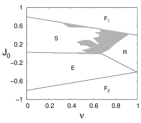
Figure 1: Phase diagram of stationary states for $c=10$ condensed patterns, $\alpha=0=T$ and initial overlap $m^{0}_{\mu}=0.4\delta_{\mu 1}$ ($\mu=1,\dots,c$). $R$ is a retrieval phase, $S$ is a phase of symmetric-like states, $E$ is a phase of period-two cycles, the grey area is a phase of correlated fixed-point states, $F_{1}$ and $F_{2}$ are phases of frozen-in fixed-point and period-two cyclic states, respectively.

popular $m^{0}_{1}=1$ which favours the retrieval phase is to be within the basin of attraction of the other phases of interest for convenient values of $J_{0}$.

We consider in this work $c=10$ condensed patterns in all the cases studied, which is suitable due to the following. First, an interesting sequence for associative-memory tasks should not be too short. Second, we expect that already for a value of $c$ of this size the phase diagrams should only exhibit small quantitative differences in the phase boundaries for different values of $c$, guided by the results for the feed-forward network [30]. Third, we are interested in fixed-point correlated states [3, 4], characterised by well-defined correlation coefficients $C_{d}$ that decrease down to a vanishingly small value for the largest $d$ which should not be too small.

Although only few results can be derived analytically (see below) due to the complexity of the problem, all the features of the phase diagrams can be obtained numerically for $\alpha=0$. We show first the results in that case for the stationary behaviour obtained by means of the iteration of (19) and (20) until a stationary overlap vector $m$ is reached. The $(\nu,J_{0})$ phase diagram of stationary states in the absence of noise ($\alpha=0=T$) is shown in figure 1. Given a value of $\nu$ (which defines a model) and the initial overlap with the condensed patterns that specifies the basins of attraction of the phases of interest, the size and the sign of the self-interaction $J_{0}$ yields the various stationary phases as indicated. The variety of the phases is also investigated studying the behaviour of the system as a function of the model parameter $\nu$, for a given $J_{0}$.

For large values of $|J_{0}|$, there is a phase $F_{1}$ of frozen-in fixed-points for positive $J_{0}$, with an overlap $m_{\mu}=0.4\,\delta_{\mu 1}$ ($\mu=1,\dots,c$) that stays the same as the initial overlap for all times, and there is a phase $F_{2}$ of frozen-in cycles for negative $J_{0}$, with an overlap $m_{\mu}^{t}=(-1)^{t}0.4\,\delta_{\mu 1}$ ($\mu=1,\dots,c$) that keeps switching between the initial overlap and its opposite. The phase boundaries of $F_{1}$ and $F_{2}$ can be derived analytically from (19) and (20) in the $T\rightarrow 0$ limit iterating the condensed overlaps at consecutive times. Writing the initial overlap as $m^{0}_{\mu}=m^{0}_{\lambda}\delta_{\mu\lambda}$ ($\mu=1,\dots,c$), for a general $m^{0}_{\lambda}$ $(0\leq m^{0}_{\lambda}\leq 1)$, this yields first an expression for $m^{1}_{\lambda}$ at the first time step in terms of $J_{0}$, $\nu$ and $m^{0}_{\lambda}$. The conditions that $m^{1}_{\lambda}=m^{0}_{\lambda}$ or $m^{1}_{\lambda}=-m^{0}_{\lambda}$ (the case for $F_{1}$ or $F_{2}$, respectively) are

$$J_{0}>m^{0}_{\lambda}(2-\nu)\,\,\,,\,\,\,\rm phase\,\,F_{1}$$ (23)

$$J_{0}<m^{0}_{\lambda}(\nu-2)\,\,\,,\,\,\,\rm phase\,\,F_{2}\,\,\,,$$ (24)

which are independent of $c$. These conditions also lead to $m^{1}_{\lambda\pm n}=0$ ($n=1,\dots,c-1$) which ensures that the network state does not switch from one condensed pattern to another. The same relation $m^{1}_{\mu}=\pm m^{0}_{\lambda}\delta_{\mu\lambda}$ ($\mu=1,\dots,c$) holds from any time-step to the next one giving rise to the phase boundaries of the frozen-in states. In phases $F_{1}$ and $F_{2}$ the system is not useful for information processing but, as will be seen below, the frozen-in states become destabilised in the presence of synaptic noise ($T>0$) and, eventually, lead to dynamically useful fixed-point or oscillating states.

In figure 1 there is a phase $R$ of retrieval fixed-point states for large $\nu$ that reflects the dominance of the Hebbian synapses, with stationary overlaps $m_{\mu}=\delta_{\mu 1}$ ($\mu=1,\dots,c$). The upper and lower phase boundaries of $R$ end at $J_{0}=\pm 0.4$ for $\nu=1$ which has been obtained analytically before for Little’s model in the absence of noise [22, 25]. A phase $S$ of symmetric or symmetric-like states of equal or similar overlap components, respectively, appears for not too large $J_{0}\geq 0$. This phase exhibits a succession of multiple discontinuous transitions of the overlap vector $m$ for intermediate values of $\nu$ that will be shown below in connection with the phase of correlated states, which is the grey area in the figure 1. It is appropriate to note here that the latter is a phase that arises from the competition between sequential and Hebbian processing and it is not present in Little’s model with pure Hebbian synapses. There is also a phase $E$ of period-two cycles with $m_{\mu}^{t+2}=m_{\mu}^{t}$ for $\mu=1,\dots,c$ mostly for negative $J_{0}$, as shown below in figure $2$ for one of the overlap components. Phase $E$ exhibits a similar behaviour as that in phase $S$ with multiple transitions but now to a variety of period-two cycles, in place of fixed-point states.

In figure 2 we show the period-two cyclic behaviour within phase $E$ for a single component, the other components behave in a similar way, for a typical $\nu=0.3$ and two negative values of $J_{0}$ within that phase, as indicated. In the upper part of the phase the stationary oscillation is between positive overlaps and in the lower part the oscillation is between $\pm m$.

(a) $\,J_{0}=-0.1$.

(b) $\,J_{0}=-0.3$.

Figure 2: Evolution of a single overlap (the other components behave in a similar way) in phase $E$ for $\nu=0.3$, initial overlap $m^{0}_{\mu}=0.4\delta_{\mu 1}$ and $\alpha=0=T$ in (a) the upper part of the phase with $J_{0}=-0.1$, and in (b) the lower part with $J_{0}=-0.3$.

(a) $\,J_{0}=0.2$.

(b) $\,\nu=0.6$.

Figure 3: Multiple transitions of one of the overlap components within the whole range of $\nu$ (a) and correlation coefficients $C_{d}$ defined in the text for various values of $J_{0}$ (b). Both figures were generated for $c=10$, $\alpha=0=T$ and initial overlap $m^{0}_{\mu}=0.4\delta_{\mu 1}$ ($\mu=1,\dots,c$).

The fixed-point solutions for one of the overlap components at $\alpha=0=T$ for a typical $J_{0}=0.2$ in phase $S$ and the whole range of $\nu$ is shown in figure 3(a). There is a finite number of bifurcations at specific values of $\nu$, in both the white and gray regions in that phase ending at the retrieval phase with $m_{1}=1$. All the other overlap components follow a similar behaviour with transitions not necessarily of the same size but at the same values of $\nu$. We have studied the fixed-point solutions in both symmetric and correlated states calculating the correlation coefficients $C_{d}$ as a function of the distance $d$, as shown in figure 3(b) for a fixed $\nu=0.6$ and different values of $J_{0}$, as indicated. Either $C_{d}$ decreases to a finite value, which is typical of symmetric-like fixed-points, or $C_{d}$ decreases to zero, which is a characteristic of correlated states. The numerical criterion chosen for the latter employed in the construction of the gray region of figure 1 is that $C_{5}<0.02$ for the maximum distance $d=5$. The non-monotonic behaviour of $C_{d}$ with $J_{0}$ reflects the reentrance region to the phase of correlated states in figure 1.

Figure 4: Phase diagram of stationary states for $c=10$, $\alpha=0$, $T=0.2$ and initial overlap $m^{0}_{\mu}=0.4\,\delta_{\mu 1}$ ($\mu=1,\dots,c$). $R$ is a retrieval phase, $S$ is a phase of symmetric-like states, $P$ is a paramagnetic phase, the regions $D$ are phases of correlated fixed-point states and $E_{1}$ and $E_{2}$ are phases of cyclic states.

In order to illustrate the role of synaptic noise on the behaviour of the network, we show in figure 4 the $(\nu,J_{0})$ phase diagram of stationary states for $\alpha=0$ and $T=0.2$. For $\nu\approx 1$, the model has a similar behaviour to that of Little’s model [22, 25]. There is a retrieval phase $R$ with $\mbox{\boldmath$m$}\simeq(m_{1},0,\dots,0)$ and $m_{1}$ assuming values in the range $0.9\lesssim m_{1}\lesssim 1$, depending on the parameters $\nu$ and $J_{0}$. The frozen-in cyclic states in the phase $F_{2}$ at $T=0=\alpha$ become destabilised by synaptic noise for all $\nu$. For the larger $\nu$ they go into a paramagnetic phase with $\mbox{\boldmath$m$}=0$ and for the smaller $\nu$ they become period-two cycles with overlaps that evolved from the initial value. The cyclic states in region $E_{1}$ are reminiscent of those in the feed-forward network [30], with each overlap component oscillating between a larger and a smaller positive value. In fact, for $\alpha=0=J_{0}$ we recover the results of [30], since in this case the equations for the order parameters are precisely the same in the layered and in the recurrent networks. The overlap components in phase $E_{2}$ are $m^{t}_{\mu}=(-1)^{t}m_{\mu}$, each one exhibiting usually a different amplitude $m_{\mu}$. The frozen-in states in phase $F_{1}$ for $\alpha=0=T$ are destabilised by synaptic noise and become symmetric or symmetric-like states in phase $S$. This is now a phase that ends at two phases of correlated fixed-point solutions in the two disjoint regions $D$, that differ in the rate at which $C_{d}$ goes to zero.

Figure 5: Phase diagram of stationary states for $c=10$, $\alpha=0$, $J_{0}=-0.2$ and initial overlap $m^{0}_{\mu}=0.4\delta_{\mu 1}$ ($\mu=1,\dots,c$). The phases are those of figure 4.

In the lower region $D$, we have $C_{d}\approx 0$ for $d=3$ whereas in the upper region $D$, $C_{d}\approx 0$ for $d=5$. As can be seen from figure 4, the range of values of $\nu$ where the network evolves to correlated fixed-point states can be enhanced by an increase of $J_{0}$.

To illustrate the robustness of the different phases with respect to synaptic noise, we show in figure 5 the $(\nu,T)$ phase diagram for $\alpha=0$ and a small $J_{0}=-0.2$.

Figure 6: Dynamics of one overlap component $m^{t}_{1}$ in the cyclic phase $E_{1}$ for $\alpha=0.01$ (a), and stationary overlap for increasing stochastic noise $\alpha$ with transition to the symmetric-like phase $S$ at $\alpha\approx 0.06$ (b), both for $c=10$, $T=0.2$, $J_{0}=-0.02$, $\nu=0.1$ and initial overlap $m^{0}_{\mu}=0.4\delta_{\mu 1}$ ($\mu=1,\dots,c$). These results were generated by the Eissfeller-Opper procedure with $N_{T}=5\times 10^{5}$ trajectories.

Although the oscillation amplitudes of the overlap components in phases $E_{1}$ and $E_{2}$ decrease with increasing $T$, the cyclic solutions are stable even for a relatively large synaptic noise.

We consider now the effects of stochastic noise due to a macroscopic number of patterns, $p=\alpha N$, employing the procedure of Eissfeller and Opper [32].

Figure 7: Dynamics of $m^{t}_{1}$ in the cyclic phase $E_{2}$ for $c=10$, $J_{0}=-0.3$, $\nu=0.1$, $T=0.2$, initial overlap $m^{0}_{\mu}=0.4\delta_{\mu 1}$ ($\mu=1,\dots,c$) and two levels of stochastic noise: $\alpha=0.5$ (crosses) and $\alpha=0.7$ (circles). These results were generated by the Eissfeller-Opper procedure with $N_{T}=5\times 10^{5}$ trajectories.

Since the construction of a phase diagram using this method is a prohibitive task due to the slow dynamics for finite $\alpha$ [25], we concentrate on the stability of some typical states. First we study the cyclic states favoured by dominating sequential synapses, that is for small $\nu$. In figures 6 and 6 we illustrate, respectively, the dynamics of $m_{1}^{t}$ and the stability to stochastic noise of a stationary overlap component (the other components behave in a similar way), both for a state in phase $E_{1}$, when $J_{0}=-0.02$, $\nu=0.1$ and $T=0.2$. Figure 6 shows, for $\alpha=0.01$, that $m_{1}^{t}$ keeps oscillating between the upper and lower values at consecutive time-steps without any significant variation in the amplitude with the asymptotic state being reached for $t\sim 40$ time steps, suggesting that the cyclic states in phase $E_{1}$ are stationary states of the network dynamics for small values of $\alpha$. The cycles decrease in amplitude with increasing $\alpha$ within that phase and change into symmetric-like states for larger $\alpha$, as shown in figure 6.

The cyclic states in phase $E_{2}$ turn out to be stable for higher stochastic noise as shown in figure 7 by the dynamics of $m_{1}^{t}$ for $J_{0}=-0.3$, $\nu=0.1$, $T=0.2$ and two values of $\alpha$. Indeed, for $\alpha=0.5$ the overlap component keeps oscillating with no change in the amplitude after a transient period, indicating stability to stochastic noise, whereas for $\alpha=0.7$ the amplitude is already decreasing, indicating that the cycles are unstable for that load of patterns. The reason for the increased robustness to stochastic noise of the cycles in phase $E_{2}$, in contrast to those in phase $E_{1}$, is that the former are deeper in the cyclic region, with a larger negative $J_{0}$ for the same initial overlap $m_{\mu}^{0}$. We comment in the last section on the relative robustness to stochastic noise of both cyclic phases.

Figure 8: Dynamics of $m^{t}_{1}$ in the lower phase $D$ of correlated fixed-point states for $c=10$, $J_{0}=-0.25$, $\nu=0.83$, $T=0.005$, initial overlap $m^{0}_{\mu}=0.4\delta_{\mu 1}$ ($\mu=1,\dots,c$) and two levels of stochastic noise: $\alpha=0.006$ (crosses) and $\alpha=0.01$ (circles). These results were generated by the Eissfeller-Opper procedure with $N_{T}=5\times 10^{5}$ trajectories.

We consider next the stability of correlated fixed-point states in the presence of stochastic noise which are expected for dominating Hebbian synapses in the presence of sequential interactions and we resort again to the EO procedure. The dynamics of $m^{t}_{1}$ up to $t=300$ time steps was studied for a state within each region $D$ of figure 4. In figure 8 are shown results in the lower region $D$ with $\nu=0.83$, $J_{0}=-0.25$, and $T=0.005$ in order to extract mainly the effects of stochastic noise for two values of $\alpha$. The upper curve, for $\alpha=0.006$, indicates that the correlated fixed-point state is stable with a stationary overlap vector given by $\mbox{\boldmath$m$}\simeq(0.75,0.25,0,\dots,0,0.25)$. This state is already unstable for a somewhat larger $\alpha=0.01$, as suggested by the lower curve, since the overlap $m^{t}_{1}$ is decreasing towards a value that is quite different from $m_{1}\simeq 0.75$. In fact, we obtained an overlap vector given approximately by $\mbox{\boldmath$m$}\simeq(0.34,0.30,0.21,0.14,0.09,0.07,0.09,0.14,0.20,0.28)$, indicating that the network is evolving to a symmetric-like state.

We have also investigated the stability of states in the upper region $D$ and in the retrieval phase, and found similar results to those in the lower $D$ region, in the first case, and results reminiscent to those for Little’s model, in the second case, indicating stability for small values of $\alpha$.

5 Summary and conclusions

The generating functional approach has been used in this work to study the synchronous dynamics, the stationary states and the transients of a recurrent neural network model with synapses generated by the competition between symmetric sequence processing and Hebbian pattern reconstruction. Either the numerical procedure of Eissfeller and Opper, based on the GFA, to simulate paths of single-spin states or a simpler alternative procedure have been used in this work to obtain results in the presence or absence of stochastic noise due to the load of a macroscopic number of patterns. There is a single time scale in the dynamics (the step of unit size) leading to both fixed-point and cyclic behaviour of period two. The latter arises from the synchronous updating of all units at every time step and it is enhanced by two features: the sequential interactions and the self-interaction of the units. The mean-field dynamics done here allows us to study the stability of the fixed-point and cyclic states as well as the transitions between them.

In distinction to Little’s model (the case $\nu=1$ of purely Hebbian synapses) where the cycles of period two only appear as frozen-in states in the absence of noise and become destabilised by synaptic or stochastic noise, there appear now in the case where $0\leq\nu<1$ also stable dynamic cycles of period two, either with or even without noise. These are cycles that evolve from the initial overlap to a stationary state, and they appear in a large region of the phase diagram.

The retrieval behaviour and the fixed-point correlated states are also enhanced by the presence of a self-interaction and in this work we investigated the changes in the phase diagrams due to that interaction. Phase diagrams of stationary states were obtained in this work and it was shown that fixed-point correlated states are clearly separated from both phases of cyclic states already for a small but finite synaptic noise, independently of the size (and even in the absence) of a self-interaction. This suggests, within the limited conclusions that can be drawn from an attractor neural network model, that there should be no interference of the oscillating states produced by the synchronous dynamics with the correlated fixed-point states that are crucial in visual task experiments.

We comment, next, on the last summation in the synaptic interaction given by (3), which is responsible for the noise term in the local field $h_{i}^{t}$. One may consider a more general form $\frac{1}{N}\sum_{\mu,\,\rho>c}^{p}\xi_{i}^{\mu}B_{\mu\,\rho}\xi_{j}^{\rho}$  with an interaction matrix of the same form as (11) for the condensed part,

$$B_{\mu\rho}=b\delta_{\mu,\,\rho}+(1-b)\,(\delta_{\mu,\,\rho+1}+\delta_{\mu,\,\rho-1})\,\,$$ (25)

with $0\leq b\leq 1$, which could be equal to $\nu$. The case we considered here, for simplicity, is a Hebbian noise with $b=1$. The more general form has been used in the case of the layered feed-forward network [30] and one may infer from the results of that work the qualitative changes on the results presented here when $b=\nu$. It turns out that the pure Hebbian case underestimates slightly the storage capacity of the fixed-point states for large values of $\nu$. On the other hand, the storage capacity for almost pure cyclic behaviour, with small $\nu$, is overestimated by a pure Hebbian noise, and this is one of the reasons for the large value of $\alpha$ for which the cyclic states are still stable in both cyclic phases $E_{1}$ and $E_{2}$, as found in section 4.

Finally, there are a few features of the model which are worth pointing out. First, is that the results obtained with the symmetric interactions $J_{ij}$ in (3), are quite different from those for Little’s model. One of these results is the presence of fixed-point correlated states, another one is the presence of stable cycles in phases $E_{1}$ and $E_{2}$, in distinction to the absence of cycles in Little’s model with noise. Furthermore, excitatory self-interactions enhance fixed-point correlated states as shown by the enlarged upper part of the $D$ phase. Also, inhibitory self-interactions are not only responsible for the enhancement of the fraction of flipping spins, a feature that is known from Little’s model, but even for the presence of fixed-point correlated states as demonstrated by the lower part of the $D$ phase. The presence of the various stationary states shown in this work depends on the relationship between the self-interaction $J_{0}$, the initial overlap $m_{\mu}^{0}$ and the value of $\nu$. These quantities shape the basins of attraction of the simplest stationary states and other states could be considered with alternative initial states if necessary. An interesting extension of this work would be to consider random self-interactions.

References

References

- [1] Sompolinsky H and Kanter I 1986 Phys. Rev. Lett.57 2861
- [2] Coolen A C C and Sherrington D 1992 J. Phys. A: Math. Gen.25 5493
- [3] Griniasty M, Tsodyks M V and Amit D J 1993 Neural Computation 5 1
- [4] Cugliandolo L F and Tsodyks M V 1994 J. Phys. A: Math. Gen.27 741
- [5] Whyte W, Sherrington D and Coolen A C C 1995 J. Phys. A: Math. Gen.28 3421
- [6] Düring A, Coolen A C C and Sherrington D 1998 J. Phys. A: Math. Gen.31 8607
- [7] Kitano K and Aoyagi T 1998 J. Phys. A: Math. Gen.31 L613
- [8] Fukai T, Kimoto T, Doi M and Okada M 1999 J. Phys. A: Math. Gen.32 5551
- [9] Laughton S N and Coolen A C C 1994 J. Phys. A: Math. Gen.27 8011
- [10] Yong C, Yinghai W and Kongqing Y 2001 Phys. Rev.E 63 041901
- [11] Coolen A C C 2001 Handbook of Biological Physics IV: Neuro-Informatics and Neural Modeling ed F Moss and S Gielen (Amsterdam: Elsevier) p 619
- [12] Laughton S N and Coolen A C C Phys. Rev.E 51 2581
- [13] Kawamura M and Okada M 2002 J. Phys. A: Math. Gen.35 253
- [14] Theumann W K 2003 Physica A 328 1
- [15] Mimura K, Kawamura M and Okada M 2004 J. Phys. A: Math. Gen.37 6437
- [16] Uezu T, Hirano A and Okada M 2004 J. Phys. Soc. Japan 73 867
- [17] Chen Y, Zhang P, Yu L, Zhang S 2008 Phys. Rev.E 77 016110
- [18] Laughton S N and Coolen A C C 1995 J. Stat. Phys. 80 375
- [19] Buzsaki G Rhythms of the Brain (New York: Oxford University Press)
- [20] Little W A 1974 Math. Biosci. 19 101; Little W A and Shaw G L 1978 Math. Biosci. 39 281
- [21] Fontanari J F and Köberle R 1987 Phys. Rev.A 36 2475; Fontanari J F and Köberle R 1988 J. Phys. France 49 13; Fontanari J F and Köberle R 1988 J. Phys. A: Math. Gen.21 L259
- [22] Fontanari J F 1988 PhD Thesis University of São Paulo (São Carlos, Brazil)
- [23] Bollé D and Busquets Blanco J 2005 Eur. Phys. J. B 47 281
- [24] Bollé D, Erichsen Jr R and Verbeiren T 2006 Physica A 368 311
- [25] Metz F L and Theumann W K 2008 J. Phys. A: Math. Gen.41 265001
- [26] Miyashita Y and Chang H S 1988 Nature 331 68
- [27] Miyashita Y 1988 Nature 335 817
- [28] Brunel N 1994 Network: Comput. in Neural Syst. 5 449
- [29] Mongillo G, Amit D J and Brunel N 2003 European Journal of Neuroscience 18 2011
- [30] Metz F L and Theumann W K 2007 Phys. Rev.E 75 041907
- [31] De Dominicis C 1978 Phys. Rev.B 18 4913
- [32] Eissfeller H and Opper M 1992 Phys. Rev. Lett.68 2094; Eissfeller H and Opper M 1994 Phys. Rev.E 50 709
- [33] Verbeiren T 2003 PhD thesis K. U. Leuven (Leuven, Belgium)