Statistics of small scale vortex filaments in turbulence

Abstract

We study the statistical properties of coherent, small-scales, filamentary-like structures in Turbulence. In order to follow in time such complex spatial structures, we integrate Lagrangian and Eulerian measurements by seeding the flow with light particles. We show that light particles preferentially concentrate in small filamentary regions of high persistent vorticity (vortex filaments). We measure the fractal dimension of the attracting set and the probability that two particles do not separate for long time lapses. We fortify the signal-to-noise ratio by exploiting multi-particles correlations on the dynamics of bunches of particles. In doing that, we are able to give a first quantitative estimation of the vortex-filaments life-times, showing the presence of events as long as the integral correlation time. The same technique introduced here could be used in experiments as long as one is capable to track clouds of bubbles in turbulence for a relatively long period of time, at high Reynolds numbers; shading light on the dynamics of small-scale vorticity in realistic turbulent flows.

Vorticity dynamics, in general, and vortex filaments, in particular, have been the subject of many theoretical, phenomenological and experimental studies from the turbulent community, both applied and theoretical saffman ; frisch ; moffat ; greg . The transport of particulate by fluid flows is an ubiquitous phenomenon in nature and in industrial applications alike. According to their inertia properties particles respond differently to fluctuations of the advecting -Eulerian- velocity field producing locally non homogeneous concentration, a phenomenon dubbed as preferential concentration tb2009 ; eaton . As an example of such differential response, it has been clearly shown in the past that heavy particles tend to be expelled from high vorticity regions, while light particles tend to concentrate in regions where vorticity is higher tb2009 . Thanks to their strong property to concentrate in high vorticity regions, very light particles (i.e. small bubbles in water) have been used to visualize small scale vortex filaments douady:1991 ; bonn:1993 . The strong tendency of light particles to concentrate in vortex filaments has been quantified also measuring the fractal dimensions of their dynamical attractor jimenez . Similar phenomena, based on complex response of microscopic hydrogen particles in quantum fluids, have also been exploited recently to visualize quantized vortices nature .

In the present work we will focus on the dynamics of light particles and will study in detail the connection between their dynamics and the one of small scale vortex filaments moffat .

The data used for this study come from Direct Numerical Simulation (DNS) of 3D fully periodic Navier-Stokes eqs plus particles. Indeed, together with the Eulerian field we integrated the Lagrangian evolution of particles by mean of one of the simplest, yet nontrivial, model of dilute, passively advected, suspensions of spherical particles as described in Refs. maxey:1983 ; auton:1988 :

$${{{\rm d}\bm{x}}\over{{\rm d}t}}=\bm{v}\,,\qquad{{{\rm d}\bm{v}}\over{{\rm d}t}}=\beta\,{{{\rm D}\bm{u}}\over{{\rm D}t}}+{1\over{\tau_{p}}}(\bm{u}-\bm{v})\,,$$ (1)

In the above equation $\bm{x}(t)$ and $\bm{v}(t)$ denote the particle position and velocity respectively, $\tau=a^{2}/(3\beta\nu)$ is the particle response time, $a$ is the particle radius and $St=\tau_{p}/\tau_{\eta}$ is the Stokes number of the particle and $\beta=3\rho_{f}/(\rho_{f}+2\rho_{p})$ is related to the contrast between the density of the particle, $\rho_{p}$, and that of the fluid, $\rho_{f}$. The incompressible fluid velocity $\bm{u}(\bm{x},t)$ evolves according to the Navier-Stokes equations :

$${\rm D}_{t}\bm{u}\equiv\partial_{t}\bm{u}+\bm{u}\cdot\bm{\nabla}\bm{u}=-\bm{\nabla}p+\nu\Delta\bm{u}+\bm{f}\,.$$ (2)

where $p$ denotes the pressure and $\bm{f}$ an external forcing injecting energy at a rate $\epsilon=\langle\bm{u}\cdot\bm{f}\rangle$. Eqn. (2) is evolved by means of a pseudo-spectral code for the fluid part with a second order Adams-Bashforth integrator, also used for the –millions of– particles evolving according to the dynamics (1), where the fluid velocity at the particle position, $\bm{u}(\bm{x}(t),t)$, was obtained by means of a tri-linear interpolation mazzitelli:2003 ; biferale:2004g . Energy was injected maintaining constant the spectral content of the first two shells in Fourier space. We report data coming from two sets of simulations with $N^{3}=128^{3}$ and $N^{3}=512^{3}$ collocation points, corresponding to $\mathrm{Re}_{\lambda}\simeq 80$ and $\mathrm{Re}_{\lambda}\simeq 180$, respectively. We focus mainly on very light particles, in the limit of $\rho_{p}\rightarrow 0$ ($\beta\rightarrow 3$ ) and on tracers evolving with the local Eulerian velocity field $\dot{\bm{x}}(t)={\bm{u}(\bm{x}(t),t)}$.

Inertial particles are not distributed homogeneously in the volume, centrifugal forces tends to concentrate light particle inside strong elliptical regions (with high vorticity) and heavy particles in hyperbolic regions, typical of intense shear. One thus expects different temporal correlations between particle trajectories and the underlying topology of the carrier flow. The local topology of the Eulerian flow is defined in terms of the symmetric and anti-symmetric component of the gradients $A_{ij}=\partial_{i}u_{j}$, hence there is an intimate link between the statistics of energy dissipation and/or enstrophy with particles evolution yeung:2007 ; luthi:2005 ; guala:2005 .

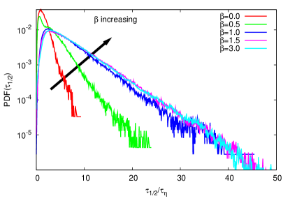
Figure 1: PDF of halving–times (see text) for various density ratios, $\beta$, at fixed $St\sim 0.5$, conditioned on the initial value of the vorticity magnitude to be larger than a given threshold. As $\beta$ increases the PDFs show larger and larger tails, suggesting that lighter particles are probing regions of high and stable vorticity.

To give an idea of this effect, we show in Fig. 1 the conditional probability distribution of the halving times, $\tau_{1/2}$, of the vorticity magnitude along particle trajectories. The vorticity halving time is defined, given a time $t$, as the first time lag after which the vorticity has becomes $1/2$ larger or smaller than the initial value, $\tau_{1/2}(t)=min(\tau|\omega(t+\tau)/\omega(t)=1\pm 1/2)$. The PDFs are conditioned in such a way that the vorticity magnitude at the reference time $t$ is greater than a given threshold (for the case in Fig. 1, we chose this value to be $5\omega_{rms}$; indeed the shape of the PDFs does not change significantly for higher values of the threshold). As one can see from the inset of Fig. 1, for a given Stokes, $St\sim 0.5$, at changing the density contrast, $\beta$, one moves towards higher and higher probability to observe long halving times, i.e. light particles tend to live in regions of high and stable vorticity.

Stable vortex structures, chaotically advected by turbulent flows, should therefore play the role of attractive sinks in the dynamics. Larger their lifetime will be, larger inhomogeneous bubble distribution will develop. To quantify better the clustering properties of light particles, we start from studying the statistics of the largest Lyapunov exponent, $\lambda_{1}$. It is known that clustering and inertia may affect the whole distribution of Lyapunov exponents. One would expects that inertia reduces the tendency for particles pairs to separate. Indeed, a small tendency toward a reduction of the Lyapunov exponent at increasing the Stokes number has been reported for heavy particles bec_et_al_pof:2006 , similar results have also been obtained in random flows duncan-mehlig-prl . Even more interesting is the study of the whole probability distribution of the largest finite-time Lyapunov exponent (FTLE), $\gamma_{1}(T)$ defined as: $\gamma_{1}(T)=\frac{1}{T}\log(R(T,t)/R(0,t))$ where $R(T,t)$ is the separation of two particles at time $t+T$ starting from a separation $R(0,t)$ at time $t$. For large times, the distribution of FTLE is expected to follow a large-deviation form: $p_{T}(\gamma_{1})\propto\exp[-TS(\gamma_{1})]$, where the Cramér function, $S(\gamma_{1})$ is a non-negative convex function vanishing for $\gamma_{1}=\lambda_{1}$. In Fig. 2 we report the Cramér function at $T=190\tau_{\eta}$ for the case of light particles $\beta=3,St\sim 1.2$ compared with the one obtained for tracers. As one can see there are two remarkable effects. First, the minimum for the case of light particles is achieved for a value much smaller than the one for the tracers, precisely $\gamma_{1}\tau_{\eta}\sim 0.04$ for bubbles and $\gamma_{1}\tau_{\eta}\sim 0.14$ for tracers. Second light particles show a remarkably high probability to have pairs that do not separate at all, even for long time lapses, i.e. there are many events in the left tail of the Cramér function which have a negative FTLE. The global average properties, however, remains chaotic, i.e. with probability one all couples separate at long times. The Kaplan-Yorke dimension for the family of light particles shown in Fig. 2 is $D_{KY}=1.3\pm 0.3$ calza .

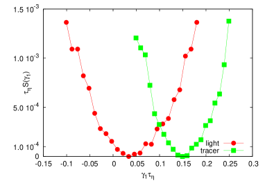
Figure 2: Cramér entropy for light particles and tracers. The function, for the case of light particles, is shifted towards lower values (the maximum Lyapunov exponent where $S(\gamma_{1})$ attains its minimum is smaller than the one for tracers) and shows larger tails (thus suggesting a higher degree of intermittency). There is a non–negligible fraction of events (left tail of the red curve) with couples of particles that do not separate at all (absent in the tracers case).

The observation that such small-scales strong clustering properties are correlated to the topology of the flow structures at the same scales suggests the possibility to use light particles to study statistical properties of small-scales vortex filaments in turbulence.

The identification of small scale vortex filaments is an extremely daunting task. An analysis of the Eulerian fields would require the detection of isosurfaces of vorticity (larger than some prescribed threshold): a method problematic if not for the larger and most intense structures jimenez . Furthermore to analyze the temporal evolution of vortex filaments one would also need to track three dimensional structures not only in space, but also to follow their evolution in time by repeating the same analysis at each Eulerian time step.

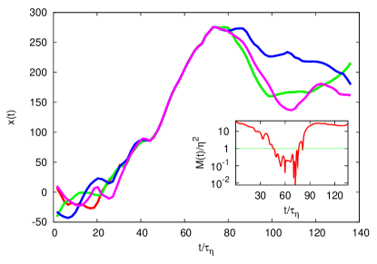
Figure 3: Evolution of the trajectory of different light particles entering in a small scale vortex filament and then separating again. In the inset it is shown the behavior of the momentum of inertia of the particles cloud. At entering (exiting) from the vortex filament an abrupt –notice the log scale– decrease (increase) of the signal allows to sharply define the life–time of the vortex filament.

Our original proposal here is to use multi-particles correlation to extraordinary enhance the signal-to-noise ratio associated to the identification of vortex filaments. In Fig. 3 we show the trajectories of several light particles which are attracted, in presence of favorable pressure gradients, into a vortex filament and that then separate again once the vortex filament disappears. Only the favorable pressure gradient, which tends to concentrate bubbles in the vortex core, permits such a strong clustering. Once the vortex filament breaks down, particles are released and separate explosively.

One can define the signal-to-noise (s/n) ratio for an event with $n$ particles in a volume where on average there are $\overline{n}$ as: $\mbox{SNR}={n/{\overline{n}}}$. Our goal here is to identify an observable which is very sensitive to the presence of small scale vortex filaments. With such an observable it will be possible to fix a threshold to define a birth and death time for the vortex filaments. We now outline our procedure in detail. We take a snapshot of light particles configuration (i.e. positions) at a time roughly in the middle of our numerical simulation. We divide our simulation volume into small cubes, say of size $4^{3}$ Kolmogorov scales, $\eta$, and we look for those volumes with larger particle counts. The particles residing in a volume will form what we call a bunch. We then consider the full trajectory of the particles within the several bunches that we identified. Obviously the number of particles in the different bunches will not be the same. We identify $M$ bunches with the $i$-th bunch formed by $N_{i}$ particles, then we define the center of mass of the bunch $i$ as ${\bm{x}}^{i}_{cm}(t)=({1/{N_{i}}})\sum_{j=1}^{N_{i}}{\bm{x}}_{j}(t)$ and the momentum of inertia for the same bunch of particles as: $M_{i}={1\over{N_{i}}}\sum_{j=1}^{N_{i}}\left({\bm{x}}_{j}(t)-{\bm{x}}^{i}_{cm}(t)\right)^{2}$. The physical interpretation is clear, the smaller the momentum of inertia of the bunch, the closer the particles. The important observation here is that this quantity is very sensitive to vortex filaments and displays an extraordinarily high signal/noise ratio (see inset of Figure 3). To understand this point one has to consider the fact that we find easily hundreds of particles at distances smaller than $0.1\eta$, while for an uniform distribution one would expect to find $1.4\cdot 10^{-3}$ particles per $\eta^{3}$. The probability to find a finite number of particles (even if just a few, say $3\div 4$) close inside $\eta^{3}$ is so small that if this happens it is almost surely associated to the presence of confining forces keeping the particles close-by (the probability could be estimate by means of the Poissonian distribution).
Another remarkable feature that makes the momentum of inertia of the bunch an extremely useful quantity to identify vortex filaments is the rapidity with which light particles in the neighborhood of a forming vortex filament are attracted into it. In the inset of Fig. 3 one can indeed see that particles initially separated move closer, remain very close to each other for some time, and then separate again. The extreme sharpness (rapidity) with which the momentum of inertia drops and then raises again allows to define the life-time of the vortex filament in a robust way. The life-time estimates are not much sensitive to the chosen threshold (in Fig. 3 the threshold has been set to the value 1, changing the value of the threshold is accounted into the error bars e.g. in Fig. 4).
By analyzing the statistics of all bunches, we can make an histogram of vortex filaments life–times, allowing for the first time to assess, in a quantitative way, the statistical properties of these extreme events. In Fig. 4 we show the pdf of vortex filaments life–times for $Re_{\lambda}=180$ and $80$ which happens to be an exponential with a decay rate which can be estimated of the order of $25\tau_{\eta}$ and $17\tau_{\eta}$, respectively. As already noticed in douady:1991 we do observe events as long as the integral time $T_{L}$, that in our simulation was estimated to be of the order of $50\tau_{\eta}$. Another interesting question is how particles bunches are formed, if this happens by means of a sudden attraction of close-by particles, or as the result of a sequence of successive -and rapid- bunch merge. The same question can be posed regarding the “decay” of a vortex filament. How do particles separate? To answer this question one can introduce the following quantity measuring the average distance between two particles in a bunch:

$$D^{2}_{i}={2\over{N_{i}(N_{i}-1)}}\sum_{j,k=1}^{N_{i}}\left({\bm{x}}_{j}(t)-{\bm{x}}_{k}(t)\right)^{2}$$ (3)

Should all particles be close then the histogram of the distances would be centered around a small unique value with a variance connected with the bunch size. In the event of a bunch being splitted into two separating (smaller) bunches, one would expect to see the appearance of a peak at some finite distance and a shift of the position of this peak with time. This is exactly the case in Fig. 5 where the pdf of $D^{2}_{i}$ for a given bunch is shown for 4 consecutive instants in time. A clearly visible peak can be identified and its position is shifting towards larger distances.

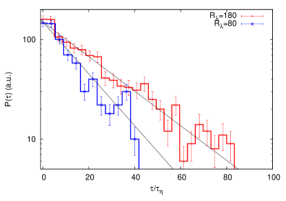
Figure 4: Probability distribution function of the life–time of vortex filaments. PDFs at two different Reynolds number, $R_{\lambda}=80$ and $R_{\lambda}=180$ respectively: in both cases it turns out that the PDF is fairly well fitted by an exponential (with a decay factor, for the highest $R_{\lambda}$, of around $20\tau_{\eta}$). In the far tail of the PDFs there are events whose life–time is of the order of the integral time. Error bars reflect the effect of changing the threshold used to determine the vortex filament time of life (see text for more details).

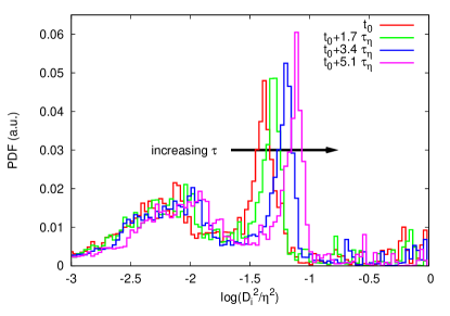
Figure 5: The probability distribution function of the average distance (squared) between pairs of particles in a bunch clearly showing a fragmentation process: a vortex filament is splitted in two and the bunch of particles is splitted in two bunches separating in time (the distance between the bunches is associated with the moving position of the peak).

One of the most intriguing features of fluid dynamics turbulence is the presence of long living coherent structures at small scales. The quantification of the statistical properties of these Eulerian structures has always proved to be one of the most difficult statistical analysis in turbulence due to the extremely low signal to noise ratio and to the need of following the evolution of structures for as long as a large scale eddy turnover time. We showed, for the first time, that the coherent dynamical properties of clouds of very light particles (bubbles) can be used to introduce an observable extremely sensitive to small scale vorticity filaments. We used this observable to quantitatively measure the probability distribution of vortex filaments life–times. We also show that the decay of a vortex filament into smaller chunks is the way particles get released from within such structures. The same observable introduced here could be used in experiments as long as one is capable to track clouds of bubbles in turbulence for a relatively long period of time, at high Reynolds numbers. Vortex dynamics is of particular importance also to study possible blow-up of Euler and Navier-Stokes equations recon as well as super-fluid dynamics koplik . Similar ideas could abridged to other domain to fortify statistical signals.

Acknowledgments We thank the DEISA Consortium (co-funded by the EU, FP6 project 508830), for support within the DEISA Extreme Computing Initiative (www.deisa.org). Data from this study are publicly available in unprocessed raw format from the iCFDdatabase (http://cfd.cineca.it).

References

- (1) P.G. Saffman, Vortex Dynamics. Cambridge University Press, Cambridge (1992).
- (2) U. Frisch, Turbulence. Cambridge University Press, Cambridge (1995).
- (3) H.K. Moffat, S. Kida and K. Ohkitani, J. Fluid Mech 259 241 (1004).
- (4) S. Chen, G. Eyink, M. Wan and Z. Xiao, Phys. Rev. Lett. 97 144505 (2006).
- (5) J.K. Eaton and J.R. Fessler, Int. J. Multiphase Flow 20, 169 (1994).
- (6) F. Toschi and E. Bodenschatz, Annu. Rev. Fluid Mech. 41, 375–404 (2009).
- (7) S. Douady, Y. Couder and M.–E. Brachet, Phys. Rev. Lett. 67, 983–986 (1991).
- (8) D. Bonn, Y. Couder, P.H.J. van Dam and S. Douady, Phys. Rev. E 47, R28–R31 (1993).
- (9) F. Moisy and J. Jiménez, J. Fluid Mech. 513, 111–133 (2004).
- (10) G. P. Bewley, D. P. Latrhop and K.R. Sreenivasan, Nature 441 588 (2006).
- (11) M.R. Maxey and J.J. Riley, Phys. Fluids 26, 883–889 (1983).
- (12) T. Auton, J. Hunt and M. Prud’homme, J. Fluid Mech. 197, 241–257 (1988).
- (13) I.M. Mazzitelli, D. Lohse and F. Toschi, Phys. Fluids 15, L5–8 (2003).
- (14) L. Biferale, G. Boffetta, A. Celani, B. Devenish, A. Lanotte and F. Toschi, Phys. Rev. Lett. 93, 064502 (2004).
- (15) P.K. Yeung, S.B. Pope, E.A. Kurth and A.G. Lamorgese, J. Fluid Mech. 582, 399–422 (2007).
- (16) B. Lthi, A. Tsinober and W. Kinzelbach, J. Fluid Mech. 528, 87–118 (2005).
- (17) M. Guala, B. Lthi, A. Liberzon, A. Tsinober and W. Kinzelbach, J. Fluid Mech. 533, 339–359 (2005).
- (18) J. Bec, L. Biferale, G. Boffetta, M. Cencini, A.S. Lanotte, S. Musacchio and F. Toschi, Phys. Fluids 18, 091702 (2006).
- (19) K. Duncan, B. Mehlig, S. stlund and M. Wilkinson, Phys. Rev. Lett 95, 240602 (2005).
- (20) E. Calzavarini, M. Kerscher, D. Lohse and F. Toschi, J. Fluid Mech. 607 13–24 (2008) .
- (21) J. Koplik and H. Levine, Phys. Rev. Lett. 71 1375 (1993).
- (22) S. Kida and M. Takaoka, Ann. Rev. Fluid Mech 26 169 (1994).