A MULTISCALE KINETIC-FLUID SOLVER WITH DYNAMIC LOCALIZATION OF KINETIC EFFECTS

Abstract

This paper collects the efforts done in our previous works [8],[11],[10] to build a robust multiscale kinetic-fluid solver. Our scope is to efficiently solve fluid dynamic problems which present non equilibrium localized regions that can move, merge, appear or disappear in time. The main ingredients of the present work are the followings ones: a fluid model is solved in the whole domain together with a localized kinetic upscaling term that corrects the fluid model wherever it is necessary; this multiscale description of the flow is obtained by using a micro-macro decomposition of the distribution function [10]; the dynamic transition between fluid and kinetic descriptions is obtained by using a time and space dependent transition function; to efficiently define the breakdown conditions of fluid models we propose a new criterion based on the distribution function itself. Several numerical examples are presented to validate the method and measure its computational efficiency.

Keywords: kinetic-fluid coupling, multiscale problems, Boltzmann-BGK equation.

1 Introduction

Many engineering problems involve fluids in transitional regimes such as hypersonic flows or micro-electro-mechanical devices. In these cases, usual fluid models (like Euler or Navier-Stokes equations) break down in localized regions of the computational domain (typically in shock and boundary layers). For such problems, using classical fluid models is generally not sufficient for an accurate description of the flow in non-equilibrium regions. However, it is not necessary to solve the Boltzmann equation—which is computationally more expensive than continuum solvers by several orders of magnitude—especially in situations where the flow is close to thermodynamical equilibrium.

For the above reasons, it is important to develop hybrid techniques which can reduce the use of kinetic solvers to the regions where they are strictly necessary (kinetic regions), leaving the simulation in the rest of the domain to a continuum or fluid solver (fluid regions). The construction of these methods involve two main problems. The first one is how to accurately identify the different regions. We refer, for instance, to the works of Wijesinghe and Hadjiconstantinou [15], Levermore, Morokoff, and Nadiga [20], and Wang and Boyd [32], in which various breakdown criteria are proposed. The second main problem is how to efficiently and correctly match the two models at the interfaces. Most of the recent methods are based on domain decomposition techniques, such as in the works of Bourgat, LeTallec, Perthame, and Qiu [3], Bourgat, LeTallec and Tidriri [4], LeTallec and Mallinger [23], Aktas and Aluru [1], Roveda, Goldstein and Varghese [27], Sun, Boyd and Candler [29], Wadsworth and Erwin [33], and Wijesinghe et al. [34]. The same domain decomposition approach has been also used in many others fields, such as, for instance, in molecular dynamics [14], in epitaxial growth [28] or for problems involving diffusive scalings [18] instead of hydrodynamic ones. We also mention the use of decompositions in velocity instead of physical space done by Crouseilles, Degond and Lemou [7] and by Dimarco and Pareschi [12].

It is important to stress that most of the mentioned methods use a static interface between kinetic and fluid regions that is chosen once for all at the beginning of the computation. However, for unsteady problems, this approach appears as somehow inadequate and inefficient, and for this reason, some automatic domain decomposition methods have also been proposed, see for example Kolobov et al. [19], or Tiwari [30, 31] and Dimarco and Pareschi [11]. We have also proposed a similar approach in [11].

In this paper, we propose a method that has similar features as the methods mentioned above: we solve the Boltzmann-BGK equation coupled with the compressible Euler equations through an adaptive domain decomposition technique. With this technique, it is possible to achieve considerable computational speedup, as compared to steady interface coupling strategies, without losing accuracy in the solution. This method is somehow an extension of our previous work [11], but several important differences must be noted. First, we introduce a new breakdown criterion which is based on a careful inspection of the distribution function. This criterion can be defined by using the macroscopic variables only, at least in fluid regions, and thus does not introduce additional expensive computations. This allows us to define kinetic regions that are small as possible. Second, we use a decomposition of the distribution function that has better properties than the one used in [11]. In fact, while it has been proved by Degond, Jin, and Mieussens [8] that the decomposition used in [11] preserves uniform flows at the continuous level, we show in this paper that this is not true in general at the discrete level, except if a quite specific and very expensive kinetic scheme is used. For this reason in the present work we use the decomposition proposed by Degond, Liu, and Mieussens [10], since it perfectly preserves uniform flows, both for the continuous and discrete cases. As in [10], we decompose the distribution function into an equilibrium part, that can be described by macroscopic fluid variables, and a perturbative non-equilibrium part. We obtain a micro-macro fluid model in which the macroscopic variables are determined by solving a fluid equation with a kinetic upscaling. This kinetic upscaling is determined by solving a kinetic equation, and is dynamically and automatically localized wherever it is necessary, by using our breakdown criterion and the transition function idea [9, 8, 10, 11]. Third, we propose an efficient numerical scheme for discretizing our micro-macro fluid model: we use a time splitting approach that has several advantages. In particular it is shown to preserve the positivity of the distribution function.

The outline of the article is the following. In section 2, we introduce the BGK equation and its properties. In section 3, we present the coupling strategy, while in section 4 the numerical scheme is described and positivity properties are analyzed. In section 5, we derive our breakdown criterion, and the final algorithm is presented. Several numerical tests are presented in section 6 to illustrate the properties of our method and to demonstrate its efficiency. A short conclusion is given in section 7. In appendix A, the differences between the present coupling strategy and the decomposition used in [8, 11] are analyzed in some details.

2 The Boltzmann-BGK model

We consider the kinetic equation

$$\partial_{t}f+v\cdot\nabla_{x}f=Q(f),$$ (1)

with the initial data

$$f(x,v,t=0)=f_{init},$$

where $f=f(x,v,t)$ is the density of particles that have velocity $v\in{}^{3}$ and position $x\in\Omega\subset{}^{3}$ at time $t>0$. The collision operator $Q$ locally acts in space and time and takes into account interactions between particles. It is assumed to satisfy local conservation properties

$$\langle mQ(f)\rangle=0$$ (2)

for every $f$, where we denote weighted integrals of $f$ over the velocity space by

$$\langle\phi f\rangle=\int_{{}^{3}}\phi(v)f(v)dv,$$ (3)

where $\phi(v)$ is any function of $v$, and $m(v)=(1,v,|v|^{2})$ are the so-called collisional invariants. It follows that the multiplication of (1) by $m(v)$ and the integration in velocity space leads to the system of local conservation laws

$$\partial_{t}\langle mf\rangle+\nabla_{x}\langle vmf\rangle=0.$$ (4)

We also assume that the functions satisfying $Q(f)=0$, referred to as local equilibrium distributions and denoted by $E[\boldsymbol{\varrho}]$, are defined implicitly through their moments $\varrho$ by

$$\boldsymbol{\varrho}=\langle mE[\boldsymbol{\varrho}]\rangle$$ (5)

In the present paper we will work with the BGK model of the Boltzmann collision operator that reads

$$Q(f)=\nu(E[\boldsymbol{\varrho}]-f).$$ (6)

With this operator, collisions are modelled by a relaxation towards the local Maxwellian equilibrium:

$$E[\boldsymbol{\varrho]}(v)=\frac{\varrho}{(2\pi\theta)^{3/2}}\exp\left(\frac{-|u-v|^{2}}{2\theta}\right),$$ (7)

where $\varrho$ and $u$ are the density and mean velocity while $\theta=RT$ with $T$ the temperature of the gas and $R$ the gas constant. The macroscopic values $\varrho$, $u$ and $T$ are related to $f$ by:

$$\varrho=\int_{{}^{3}}fdv,\qquad\varrho u=\int_{{}^{3}}vfdv,\qquad\theta=\frac{1}{3\varrho}\int_{{}^{3}}|v-u|^{2}fdv,$$ (8)

while the internal energy $e$ is defined as

$$e=\frac{1}{2\varrho}\int_{{}^{3}}|v|^{2}fdv=\frac{1}{2}|u|^{2}+\frac{3}{2}\theta.$$ (9)

The parameter $\nu>0$ is the relaxation frequency. In this paper, we use the classical choice $\nu=\mu/p$ where $\mu=\mu_{ref}(\theta/\theta_{ref})^{\omega}$ is the viscosity and $p$ is the pressure. We refer to section 6 for numerical values of $\mu_{ref}$, $\theta_{ref}$ and $\omega$.

Boundary conditions have to be specified for equation (1). Different type of conditions are used in applications: inflow, outflow, specular reflection or total accomodation. We will specify the conditions we use for every numerical test in section 6.

When the mean free path between particles is very small compared to the size of the computational domain, the space and time variables can be rescaled to

$$x^{\prime}=\varepsilon x,\ t^{\prime}=\varepsilon t$$ (10)

where $\varepsilon$ is the ratio between the microscopic and the macroscopic scale (the so-called Knudsen number). Using these new variables in (1), we get

$$\partial_{t^{\prime}}f^{\varepsilon}+v\cdot\nabla_{x^{\prime}}f^{\varepsilon}=\frac{\nu}{\varepsilon}(E^{\varepsilon}[\boldsymbol{\varrho}]-f^{\varepsilon}).$$ (11)

If the Knudsen number $\varepsilon$ tends to zero, this equation shows that the distribution function converges towards the local Maxwellian equilibrium $E^{\varepsilon}[\boldsymbol{\varrho}]$. Using this relation into the conservation laws (4) gives the Euler equations for $\boldsymbol{\varrho}$:

$$\partial_{t^{\prime}}\boldsymbol{\varrho}+\nabla_{x^{\prime}}F(\boldsymbol{\varrho})=0,$$ (12)

where $F(\boldsymbol{\varrho})=\langle vmE^{\varepsilon}[\boldsymbol{\varrho}]\rangle=(\varrho,\varrho u,\varrho e)$.

In the sequel, to give a simple description of our approach, all schemes and all algorithms are shown for the one dimensional case in velocity and physical space. The extension to the multidimensional case does not introduce any additional difficulty in the mathematical setting. We will also omit the primes wherever they are unnecessary.

3 The coupling method

In this section, we follow the work of [10] and extend the micro-macro fluid model to allow for dynamic localization of the kinetic upscaling.

3.1 Decomposition of the kinetic equation

Our method is based on the micro-macro decomposition of the distribution function: it is decomposed in its local Maxwellian equilibrium and the deviation part as

$$f=E[\boldsymbol{\varrho}]+g.$$ (13)

Because the equilibrium distribution has the same first three moments as $f$ we have

$$\langle mg\rangle=0.$$ (14)

Then it can be easily proved that the following coupled system

$$\partial_{t}\boldsymbol{\varrho}+\partial_{x}F(\boldsymbol{\varrho})+\partial_{x}\langle vmg\rangle=0$$ (15)

$$\partial_{t}g+v\partial_{x}g=-\nu g-(\partial_{t}+v\partial_{x})E[\boldsymbol{\varrho}]$$ (16)

is satisfied by $\boldsymbol{\varrho}=\langle mf\rangle$ and $g=f-E[\boldsymbol{\varrho}]$, where $F(\boldsymbol{\varrho})=\langle vmE[\boldsymbol{\varrho}]\rangle$ is the flux associated to the equilibrium state. The corresponding initial data are

$$\boldsymbol{\varrho}_{t=0}=\boldsymbol{\varrho}_{init}=\langle mf_{init}\rangle,\ \ \ \ g_{t=0}=f_{init}-E[\boldsymbol{\varrho}_{init}].$$ (17)

The converse statement is also true: if $\boldsymbol{\varrho}$ and $g$ satisfy system (15) and (16) with initial data (17), then $f=E[\boldsymbol{\varrho}]+g$ satisfies the kinetic equation (1) (see [8] for details). In the following section, starting from this decomposition, we introduce the set of equations that define the domain decomposition technique we are proposing.

3.2 Transition function

Let $\Omega_{1}$, $\Omega_{2}$, and $\Omega_{3}$ be three disjointed sets such that $\Omega_{1}\cup\Omega_{2}\cup\Omega_{3}={}^{3}$. The first set $\Omega_{1}$ is supposed to be a domain in which the flow is far from the equilibrium (the ”kinetic zone”), while the flow is supposed to be close to the equilibrium in $\Omega_{2}$ (the ”fluid zone”) and also in $\Omega_{3}$ (the ”buffer zone”). We define a function $h(x,t)$ such that

$$h(x,t)=\left\{\begin{array}[]{lll}\displaystyle 1,&\mbox{for}&x\in\Omega_{1},\\ 0,&\mbox{for}&x\in\Omega_{2},\\ 0\leq h(x,t)\leq 1,&\mbox{for}&x\in\Omega_{3}.\\ \end{array}\right.$$ (18)

Note that the time dependence of $h$ means that we account for possibly dynamically changing fluid and kinetic zones. The topology and geometry of these zones is directly encoded in $h$ and may change dynamically as well.

Next, we split the perturbation term in two distribution functions $g_{K}=hg$ and $g_{F}=(1-h)g$. The time derivatives of these functions then are

$$\partial_{t}g_{K}=\partial_{t}(hg)=g\,\partial_{t}h+h\partial_{t}g,$$

$$\partial_{t}g_{F}=\partial_{t}((1-h)g)=-g\,\partial_{t}h+(1-h)\partial_{t}g,$$

and it is therefore easy to derive the following coupled system of equations

$$\partial_{t}\boldsymbol{\varrho}+\partial_{x}F(\boldsymbol{\varrho})+\partial_{x}\langle vmg_{K}\rangle+\partial_{x}\langle vmg_{F}\rangle=0$$ (19)

$$\partial_{t}g_{K}+hv\partial_{x}g_{K}+hv\partial_{x}g_{F}=-\nu g_{K}-h(\partial_{t}+v\partial_{x})E[\boldsymbol{\varrho}]+\frac{g_{K}}{h}\partial_{t}h,$$ (20)

$$\partial_{t}g_{F}+(1-h)v\partial_{x}g_{K}+(1-h)v\partial_{x}g_{F}=-\nu g_{F}-(1-h)(\partial_{t}+v\partial_{x})E[\boldsymbol{\varrho}]-\frac{g_{F}}{1-h}\partial_{t}h,$$ (21)

with initial data

$$g_{K,t=0}=h_{t=0}g_{t=0}\,,\quad g_{F,t=0}=(1-h_{t=0})g_{t=0}\,,\quad\boldsymbol{\varrho}_{t=0}=\boldsymbol{\varrho}_{init}$$ (22)

and with $h_{t=0}=h_{init}$ and $g_{t=0}=f_{init}-E[\boldsymbol{\varrho}_{init}]$. Again, system (19–21) with initial data (22) is equivalent to system (15–16) with initial data (17) (see [8] for details).

Now assume that the flow is very close to equilibrium in $\Omega_{2}\cup\Omega_{3}$. This means that $g$ is very small in these domains and can be set to zero. Since $g=g_{F}$ in $\Omega_{2}$, we set $g_{F}=0$ in this domain. In $\Omega_{3}$, we also set $g_{F}=0$, which means that we approximate $g$ by $g_{K}$. Consequently, $g_{F}$ can be eliminated from (19–21) to get:

$$\partial_{t}\boldsymbol{\varrho}+\partial_{x}F(\boldsymbol{\varrho})+\partial_{x}\langle vmg_{K}\rangle=0$$ (23)

$$\partial_{t}g_{K}+hv\partial_{x}g_{K}=-\frac{\nu}{\varepsilon}g_{K}-h(\partial_{t}+v\partial_{x})E[\boldsymbol{\varrho}]+\frac{g_{K}}{h}\partial_{t}h,$$ (24)

with initial data

$$g_{K,t=0}=h_{t=0}g_{t=0}=h_{init}(f_{init}-E[\boldsymbol{\varrho}_{init}])\,,\quad\boldsymbol{\varrho}_{t=0}=\boldsymbol{\varrho}_{init}.$$ (25)

Note that since by definition $g_{K}$ is zero in the fluid zone $\Omega_{2}$, the kinetic equation equation (24) is solved in the kinetic and buffer zones $\Omega_{1}$ and $\Omega_{3}$ only. Indeed, in the fluid zone, we only solve (23) with $g_{K}=0$, which is nothing but the Euler equations. In the kinetic zone, we have $g_{K}=g$ and hence system (23–24) is nothing but system (15–16), which is equivalent to the original BGK equation. System (23–24) is our micro-macro fluid model with dynamically localized kinetic effects which will be used to solve multiscale kinetic problems. With this system, the distribution function $f$ is approximated by $E[\boldsymbol{\varrho}]+g_{K}$.

In the next section we describe and analyze the numerical scheme we use to discretize this system, and we compare this new model to the model used in our previous work [11].

Remark 1.

We mention here a slightly different derivation that leads to a different micro-macro model. In (20), the term $\frac{g_{K}}{h}$ can be equivalently replaced by $g_{K}+g_{F}$, since $g_{K}=hg$ by definition and also $g=g_{K}+g_{F}$. In this case, the approximation $g_{F}=0$ in $\Omega_{2}$ and $\Omega_{3}$ leads to the model:

$$\partial_{t}\boldsymbol{\varrho}+\partial_{x}F(\boldsymbol{\varrho})+\partial_{x}\langle vmg_{K}\rangle=0$$ (26)

$$\partial_{t}g_{K}+hv\partial_{x}g_{K}=-\frac{\nu}{\varepsilon}g_{K}-h(\partial_{t}+v\partial_{x})E[\boldsymbol{\varrho}]+g_{K}\partial_{t}h$$ (27)

Note that, surprisingly, this model is different from (23–24): indeed, the factor of $\partial_{t}h$ is $g_{K}$ in (26–27), while it is $\frac{g_{K}}{h}$ in (23–24). However, we only use system (23–24) in the sequel, since it can be proved to have very good properties (like positivity preservation).

4 Numerical approximation of the coupled model and its properties

First, we briefly describe a velocity discretization of the kinetic BGK equation. Then, we propose a second order in space numerical scheme for the perturbation term $g_{K}$ and for the macroscopic fluid equations. Then, we introduce a time splitting method between the transition function term and the rest of the system to compute the evolution of the perturbation function $g_{K}$. Finally, positivity property for the distribution function $f$ is analyzed in details.

4.1 Discrete velocity model for kinetic equations

Here, we replace the continuous velocity space by a bounded Cartesian grid $\mathcal{V}$ of $N$ nodes $v_{j}=j\Delta v+a$, where $j$ is a bounded index, $\Delta v$ is the grid step, and $a$ is a constant. The collisional invariants $m(v)$ are replaced by $m_{j}=(1,v_{j},\frac{1}{2}|v_{j}|^{2})$. The distribution function $f$ is approximated on the grid by $(f_{j}(t,x))_{j}$, where $f_{j}(t,x)\approx f(x,v_{j},t)$, while the fluid quantities are obtained from $f_{j}$ through discrete summations on $\mathcal{V}$:

$$\boldsymbol{\varrho}=\sum_{j}m_{j}f_{j}\,\Delta v.$$ (28)

The BGK model is then replaced by the following system of $N$ hyperbolic equations with a stiff relaxation term:

$$\partial_{t}f_{j}+v_{j}\partial_{x}f_{j}=\frac{\nu}{\varepsilon}({\cal E}_{j}[\boldsymbol{\varrho}]-f_{j}),$$ (29)

where ${\cal E}_{j}[\boldsymbol{\varrho}]$ is the approximation of the continuous Maxwellian $E[\varrho]$. Note that this approximation is not the evaluation of $E[\boldsymbol{\varrho}]$ on the grid points: in fact, to ensure conservation of macroscopic quantities and entropy decay at the discrete level, the approximated Maxwellian ${\cal E}[\boldsymbol{\varrho}_{j}]$ is defined through an entropy minimization problem that can be solved by computing the solution of a small non-linear system (we refer the reader to [21, 22] for details about this approximation).

Finally, a micro-macro system with localized upscaling can be derived from the discrete-velocity BGK equation (29), exactly as in the continous case, and we find:

$$\partial_{t}\boldsymbol{\varrho}+\partial_{x}F(\boldsymbol{\varrho})+\partial_{x}\langle vmg_{K}\rangle=0$$ (30)

$$\partial_{t}g_{K,j}+hv_{j}\partial_{x}g_{K,j}=-\frac{\nu}{\varepsilon}g_{K,j}-h(\partial_{t}+v_{j}\partial_{x}){\cal E}_{j}[\boldsymbol{\varrho}]+\frac{g_{K_{j}}}{h}\partial_{t}h,$$ (31)

with initial data

$$g_{K,j,t=0}=h_{t=0}g_{t=0,j}=h_{init}(f_{init,j}-{\cal E}_{j}[\boldsymbol{\varrho}_{init}])\,,\quad\boldsymbol{\varrho}_{t=0}=\boldsymbol{\varrho}_{init},$$

where $\langle.\rangle$ now stands for $\sum_{j}.\Delta v$.

4.2 Numerical schemes

4.2.1 Non-splitting scheme

For the space discretization, we consider a grid of step $\Delta x$ and nodes $x_{i}$, while for the time discretization, we consider the step $\Delta t$ and times $t_{n}=n\Delta t$. The unknowns $\boldsymbol{\varrho}$ and $g_{K,j}$ are approximated by $\boldsymbol{\varrho}^{n}_{i}\approx\boldsymbol{\varrho}(t_{n},x_{i})$ and $g^{n}_{K,i,j}\approx g_{j}(t_{n},x_{i})$. Now, the space and time discretization of the discrete velocity micro-macro system (30–31) is:

$$\frac{g^{n+1}_{K,i}-g^{n}_{K,i}}{\Delta t}+h_{i}^{n}\left(\frac{\phi_{i+1/2}(g_{K}^{n})-\phi_{i-1/2}(g^{n}_{K})}{\Delta x}\right)=-\frac{\nu}{\varepsilon}g^{n+1}_{K,i}$$

$$-h^{n}_{i}\left(\frac{{\cal E}[\boldsymbol{\varrho}^{n+1}_{i}]-{\cal E}[\boldsymbol{\varrho}^{n}_{i}]}{\Delta t}+\frac{\phi_{i+1/2}({\cal E}[\boldsymbol{\varrho}^{n}])-\phi_{i-1/2}({\cal E}[\boldsymbol{\varrho}^{n}])}{\Delta x}\right)+\frac{g^{n}_{K,i}}{h_{i}^{n}}\frac{h_{i}^{n+1}-h_{i}^{n}}{\Delta t}$$ (32)

where the second order numerical fluxes are defined by

$$\phi_{i+1/2}(g^{n}_{K})=v^{-}g^{n}_{K,i+1}+v^{+}g^{n}_{K,i}+\frac{1}{2}|v_{j}|\min\mod(g^{n}_{K,i}-g^{n}_{K,i-1},g^{n}_{K,i+1}-g^{n}_{K,i},g^{n}_{K,i+2}-g^{n}_{K,i})$$

with $v^{-}=v_{j}$ if $v_{j}<0$ and $v^{-}=0$ in other cases, while $v^{+}=v_{j}$ if $v_{j}\geq 0$ and $v^{+}=0$ if $v_{j}$ is negative. The same numerical flux is used for $\phi_{i+1/2}(E[\boldsymbol{\varrho}^{n}])$. Note that for simplicity, in (32) and all what follows, the discrete-velocity index $j$ is omitted, as well as the space and time dependency of $\nu$.

Note that in (32), $\boldsymbol{\varrho}^{n+1}$ is computed by using a discrete version of (30) which is explained below. Moreover, note that the last term of the right-hand side of (32) models the evolution of the transition function $h$: the new value $h^{n+1}$ depends on the equilibrium/non equilibrium state of the gas in a way that will be described in section 5. In addition, we point out that when $h_{i}^{n}=0$, equation (32) is not solved, thus the term $g^{n}_{K,i}/h_{i}^{n}$ does not lead to any computational difficulties. Finally, note that the stiff relaxation term of (32) is implicit. This allows us to use a time step which is independent of $\varepsilon$.

Now, we describe the numerical scheme for the macroscopic equation (30). This equation is discretized according to

$$\frac{\boldsymbol{\varrho}^{n+1}_{i}-\boldsymbol{\varrho}^{n}_{i}}{\Delta t}+\frac{\psi_{i+1/2}(\boldsymbol{\varrho}^{n},g^{n}_{K})-\psi_{i-1/2}(\boldsymbol{\varrho}^{n},g^{n}_{K})}{\Delta x}=0$$ (33)

where the numerical flux is an approximation of the total flux $F(\boldsymbol{\varrho},g_{K})=F(\boldsymbol{\varrho})+\langle vmg_{K}\rangle$ obtained by the second order MUSCL extension of a Lax-Friedrichs like scheme:

$$\psi_{i+1/2}(\boldsymbol{\varrho}^{n},g^{n}_{K})=\frac{1}{2}(F(\boldsymbol{\varrho}^{n}_{i},g^{n}_{K,i})+F(\boldsymbol{\varrho}^{n}_{i+1},g^{n}_{K,i+1}))-\frac{1}{2}\alpha(\boldsymbol{\varrho}^{n}_{i+1}-\boldsymbol{\varrho}^{n}_{i})+\frac{1}{4}(\sigma^{n,+}_{i}-\sigma^{n,-}_{i+1})$$ (34)

In this relation, we set

$$\sigma^{n,\pm}_{i}=\left(F(\boldsymbol{\varrho}^{n}_{i+1},g^{n}_{K,i+1})\pm\alpha\boldsymbol{\varrho}^{n}_{i+1}-F(\boldsymbol{\varrho}^{n}_{i},g^{n}_{K,i})\mp\alpha\boldsymbol{\varrho}^{n}_{i}\right)\varphi(\chi^{n,\pm}_{i})$$ (35)

where $\varphi$ is a slope limiter, $\alpha$ is the largest eigenvalue of the Euler system and

$$\chi^{n,\pm}_{i}=\frac{F(\boldsymbol{\varrho}^{n}_{i},g^{n}_{K,i})\pm\alpha\boldsymbol{\varrho}^{n}_{i}-F(\boldsymbol{\varrho}^{n}_{i-1},g^{n}_{K,i-1})\mp\alpha\boldsymbol{\varrho}^{n}_{i-1}}{F(\boldsymbol{\varrho}^{n}_{i+1},g^{n}_{K,i+1})\pm\alpha\boldsymbol{\varrho}^{n}_{i+1}-F(\boldsymbol{\varrho}^{n}_{i},g^{n}_{K,i})\mp\alpha\boldsymbol{\varrho}^{n}_{i}}$$ (36)

where the above vectors ratios are defined componentwise.

4.2.2 Time splitting scheme

Here, we propose an alternative scheme based on a time splitting between the $\partial_{t}h$ term and the other terms in the kinetic equation for $g_{K}$ (31). We will show in the next section that this method preserves the positivity of the distribution function $f=E[\boldsymbol{\varrho}]+g_{K}$ under a suitable CFL condition.

First, we solve the macroscopic equation using (33) as in the previous scheme, where the numerical fluxes are defined in (34). Now, for the kinetic equation on $g_{K}$, the time variation of $h$ only is taken into account in (31) to get the second step:

$$g^{n+\frac{1}{2}}_{K,i}=g^{n}_{K,i}+\frac{g_{K,i}^{n}}{h_{i}^{n}}(h_{i}^{n+1}-h_{i}^{n}).$$

Note that this relation can be readily simplified in

$$g^{n+\frac{1}{2}}_{K,i}=g_{K,i}^{n}\frac{h_{i}^{n+1}}{h_{i}^{n}},$$ (37)

where, again, we point out that this equation is solved only if $h^{n}_{i}\neq 0$.

In a third step, (31) is discretized without the $\partial_{t}h$ term, by using the same approximation as for the non-splitting scheme. We get:

$$\frac{g^{n+1}_{K,i}-g^{n+1/2}_{K,i}}{\Delta t}+h_{i}^{n+1}\left(\frac{\phi_{i+1/2}(g_{K}^{n+1/2})-\phi_{i-1/2}(g^{n+1/2}_{K})}{\Delta x}\right)=-\frac{\nu}{\varepsilon}g^{n+1}_{K,i}$$

$$-h^{n+1}_{i}\left(\frac{{\cal E}[\boldsymbol{\varrho}^{n+1}_{i}]-{\cal E}[\boldsymbol{\varrho}^{n}_{i}]}{\Delta t}+\frac{\phi_{i+1/2}({\cal E}[\boldsymbol{\varrho}^{n}])-\phi_{i-1/2}({\cal E}[\boldsymbol{\varrho}^{n}])}{\Delta x}\right).$$ (38)

Note that for the moment, we did not mention how the new value of the transition function $h^{n+1}$ is defined. This is done by using some criteria that are introduced in section 5. Independently of this problem, we analyze in the following section the positivity property for the distribution function.

4.3 Positivity of the distribution function for the discretized equations

In this section, we prove that the splitting scheme (37-38) preserves the positivity of $f$ under a suitable CFL condition. Another interesting property of the model here proposed, the preservation of uniform flows, will be analyzed in the appendix in comparison with different coupling strategies proposed in the recent past [8, 9, 11].

Proposition 1.

If $f^{0}\geq 0$ and $g^{0}_{K}=h^{0}(f^{0}-{\cal E}[\boldsymbol{\varrho}^{0}])$, where $\boldsymbol{\varrho}^{0}=\langle mE[\boldsymbol{\varrho}]\rangle$ and $0\leq h^{0}\leq 1$, then scheme (33–38) satisfies

$$f^{n}_{i}={\cal E}[\boldsymbol{\varrho}^{n}_{i}]+g^{n}_{K,i}\geq 0$$

for every $n$ and $i$, provided that $\Delta t$ satisfies the following CFL condition:

$$\Delta t\leq\frac{\Delta x}{\max(v_{j})}\min_{i,v_{j}}\left(\frac{g^{n+1/2}_{K,i}+h^{n+1}_{i}{\cal E}[\boldsymbol{\varrho}^{n}_{i}]}{h^{n+1}_{i}(g^{n+1/2}_{K,i}+{\cal E}[\boldsymbol{\varrho}^{n}_{i}])}\right).$$ (39)

Proof.

The idea is in fact to prove a stronger property: indeed, we can prove, by induction, that the positivity of $h^{n}_{i}{\cal E}[\boldsymbol{\varrho}^{n_{i}}]+g^{n}_{K,i}$ is preserved at any time.

First, note that this relation holds at $n=0$: from the definition of $g^{0}_{K}$, we have $h^{0}_{i}{\cal E}[\boldsymbol{\varrho}^{0}_{i}]+g^{0}_{K,i}=h^{0}_{i}f^{0}_{i}\geq 0$.

Then, we assume that this relation is satisfied for some $n$, and we prove that it is true for $n+1$. This is done in the following three steps.

Step 1.
We first use (38) (where the numerical fluxes $\phi_{i+1/2}$ are computed by the first order upwind scheme) to explicitely compute $g^{n+1}_{K,i}$ and then to obtain:

$$\begin{split}g^{n+1}_{K,i}+h^{n+1}_{i}{\cal E}[\boldsymbol{\varrho}^{n+1}_{i}]=\frac{1}{1+\nu\Delta t/\varepsilon}&\biggl{(}(g^{n+1/2}_{K,i}+h^{n+1}_{i}{\cal E}[\boldsymbol{\varrho}^{n}_{i}])-\frac{|v|\Delta t}{\Delta x}h^{n+1}_{i}(g^{n+1/2}_{K,i}+{\cal E}[\boldsymbol{\varrho}^{n}_{i}])\\ &+\frac{v^{+}\Delta t}{\Delta x}h^{n+1}_{i-1}(g^{n+1/2}_{K,{i-1}}+{\cal E}[\boldsymbol{\varrho}^{n}_{i-1}])\\ &-\frac{v^{-}\Delta t}{\Delta x}h^{n+1}_{i+1}(g^{n+1/2}_{K,{i+1}}+{\cal E}[\boldsymbol{\varrho}^{n}_{i+1}])\biggr{)}\\ &+\frac{1}{1+\varepsilon/(\nu\Delta t)}h^{n+1}_{i}{\cal E}[\boldsymbol{\varrho}^{n+1}_{i}]\end{split}$$ (40)

Now, it is clear that the sign of the left-hand side depends on the sign of $g^{n+1/2}_{K,i}+h^{n+1}_{i}{\cal E}[\boldsymbol{\varrho}^{n}_{i}]$ and $g^{n+1/2}_{K,i}+{\cal E}[\boldsymbol{\varrho}^{n}_{i}]$. These two terms are studied in step 2.

Step 2.
Here, we use the definition of $g^{n+1/2}_{K,i}$ (see (37)) to obtain $g^{n+1/2}_{K,i}+h^{n+1}_{i}{\cal E}[\boldsymbol{\varrho}^{n}_{i}]=\frac{h^{n+1}_{i}}{h^{n}_{i}}(h^{n}_{i}{\cal E}[\boldsymbol{\varrho}^{n}_{i}]+g^{n}_{K,i})$ which is non-negative (due to the induction assumption). Consequently, $g^{n+1/2}_{K,i}+h^{n+1}_{i}{\cal E}[\boldsymbol{\varrho}^{n}_{i}]$ is non-negative. Since ${\cal E}[\boldsymbol{\varrho}^{n}_{i}]\geq 0$ and $0\leq h^{n+1}_{i}\leq 1$, then we also have that $g^{n+1/2}_{K,i}+{\cal E}[\boldsymbol{\varrho}^{n}_{i}]$ is non-negative.

Step 3.
Note that step 2 shows that the last three terms of the right-hand side of (40) are non-negative. Consequently, (40) shows that $g^{n+1}_{K,i}+h^{n+1}_{i}{\cal E}[\boldsymbol{\varrho}^{n+1}_{i}]$ is non-negative if $\Delta t$ satisfies the CFL condition (39). By induction, $h^{n}_{i}{\cal E}[\boldsymbol{\varrho}^{n}_{i}]+g^{n}_{K,i}$ is non-negative for every $n$, and for every $i$ and $v$.

Finally, using again that ${\cal E}[\boldsymbol{\varrho}^{n}_{i}]\geq 0$ and $0\leq h^{n}_{i}\leq 1$, we easily deduce that ${\cal E}[\boldsymbol{\varrho}^{n}_{i}]+g^{n}_{K,i}$ is also non-negative. ∎

Remark 2.

If $g^{n}_{K,i}\geq 0$, condition (39) is less restrictive than the CFL condition $\Delta t\leq\frac{\Delta x}{\max(v_{j})}$ obtained with a classical semi-implicit scheme for the original BGK equation. On the contrary, condition (39) becomes more restrictive if the perturbation term $g^{n}_{K,i}$ is negative. However, if we assume that $g$ is small enough (e.g. ${\cal E}[\boldsymbol{\varrho}^{n}_{i}]\gg g^{n+1/2}_{K,i}$), then the factor $\frac{\Delta x}{\max(v_{j})}$ in (39) is close to 1. Indeed:

$$\left(\frac{g^{n+1/2}_{K,i}+h^{n+1}_{i}{\cal E}[\boldsymbol{\varrho}^{n}_{i}]}{h^{n+1}_{i}(g^{n+1/2}_{K,i}+{\cal E}[\boldsymbol{\varrho}^{n}_{i}])}\right)=\left(1+\frac{(1-h_{i}^{n+1})g^{n+1/2}_{K,i}}{h^{n+1}_{i}(g^{n+1/2}_{K,i}+{\cal E}[\boldsymbol{\varrho}^{n}_{i}])}\right)\simeq 1,$$ (41)

and (39) reduces to the classical CFL for transport $\Delta t\leq\frac{\Delta x}{\max(v_{j})}$.

By contrast, we justify below why we think that the non-splitting scheme (32–33) cannot preserve the positivity of $f$. Indeed, by using similar computations as the ones we did for the splitting scheme, we find:

$$f^{n+1}_{i}\geq\frac{\varepsilon/\nu}{\varepsilon/\nu+\Delta t}\left((g^{n}_{K,i}+h^{n}_{i}{\cal E}[\boldsymbol{\varrho}^{n}_{i}])-\frac{v\Delta t}{\Delta x}h^{n}_{i}(g^{n}_{K,i}+{\cal E}[\boldsymbol{\varrho}^{n}_{i}])+g_{K,i}^{n}\frac{h^{n+1}_{i}-h^{n}_{i}}{h^{n}_{i}}\right)$$

$$+\frac{\varepsilon/\nu}{\varepsilon/\nu+\Delta t}\frac{h^{n}_{i}\Delta tv}{\Delta x}(g^{n}_{K,i-1}+{\cal E}[\boldsymbol{\varrho}^{n}_{i-1}])+\frac{\Delta t}{\varepsilon/\nu+\Delta t}{\cal E}[\boldsymbol{\varrho}^{n+1}_{i}].$$

Now, it is clear that the sign of $f^{n+1}$ depends on the signs of $h^{n+1}_{i}-h^{n}_{i}$ and $g_{K}^{n}$, and hence cannot be controlled by a CFL condition on $\Delta t$.

5 Localization of Fluid-Kinetic Transitions and the Dynamic Coupling Technique

One of the key points in a domain decomposition technique for gas dynamics problems is to efficiently localize the regions where the state of the gas departs from equilibrium, so as to describe the solution with the appropriate microscopic model. In other words we look for an accurate criterion the evaluation of which is computationally inexpensive.

Here, we propose three different criteria based on the information which can be retrieved from either the kinetic distribution function or from the macroscopic variables. The way the localization of the equilibrium and non-equilibrium regions evolves is described at the end of this section.

5.1 Analysis of Microscopic and Macroscopic Criteria

5.1.1 Microscopic Criteria

In regions where the kinetic or coupled kinetic/fluid models are solved, we can use the distribution function to measure the fraction of gas particles which are not distributed according to a Maxwellian (as in [11]). In the same way, the fractions of momentum, energy, and heat flux due to the non-equilibrium flux can be measured. Consequently, in every cell where $h\neq 0$, it is possible to evaluate the parameters

$$\lambda_{1,K}=\langle|g_{K}(v)|\rangle,\ \lambda_{2,K}=\langle v|g_{K}(v)|\rangle,\ \lambda_{3,K}=\langle\frac{|v|^{2}}{2}|g_{K}(v)|\rangle,\ \lambda_{4,K}=|\langle v\frac{|v|^{2}}{2}g_{K}(v)\rangle|.$$ (42)

Note that the first three values above will be zero if we use $g_{K}$ instead of $|g_{K}|$, while the last one is in general different from zero. For compatibility with the macroscopic criterion introduced in the sequel, the definition of $\lambda_{4}$ in (42) has been preferred to the alternate definition $\lambda_{4,K}=\langle|v\frac{|v|^{2}}{2}g_{K}(v)|\rangle$. The four parameters are computed in our code with the following quadrature formula

$$\lambda_{1,K}=\sum_{j}|g_{K,j}|\Delta v,\ \lambda_{2,K}=\sum_{j}v_{j}|g_{K,j}|\Delta v,$$

$$\lambda_{3,K}=\sum_{j}\frac{|v_{j}|^{2}}{2}|g_{K,j}|\Delta v,\ \lambda_{4,K}=|\sum_{j}v\frac{|v_{j}|^{2}}{2}g_{K,j}\Delta v|,$$ (43)

where $g_{K,j}(t,x)\approx g_{K}(x,v_{j},t)$. In kinetic and buffer zones $\Omega_{1}\cup\Omega_{3}$ (where $h\neq 0$), the discrepancy between the fluid and kinetic models can be measured by the following parameters

$$\beta^{n}_{1,i,K}=\frac{\lambda^{n}_{1,i,K}}{\varrho^{n}_{i}},\ \beta^{n}_{2,i,K}=\frac{\lambda^{n}_{2,i,K}}{\varrho_{i}^{n}u_{i}^{n}},\ \beta^{n}_{3,i,K}=\frac{\lambda^{n}_{3,i,K}}{\varrho_{i}^{n}e_{i}^{n}},$$ (44)

or alternatively, we can use the value of the heat flux relatively to the value of the equilibrium energy flux

$$\beta_{4,i,K}^{n}=\frac{\lambda_{4,i,K}^{n}}{|\langle v\frac{1}{2}|v|^{2}E[\rho_{i}^{n}]\rangle|}.$$ (45)

In order to define a unique variable which permits to switch from one model to the other one in every regime and in every region ($\Omega_{i},\ i=1,2,3$), we choose $\beta_{4}$ as the breakdown parameter. Indeed, as shown below, it is possible to estimate this quantity also in fluid regimes. By using this criterion, the transition function can be defined by an appropriate function that maps $\beta_{4}$ to the interval $[0,1]$: $h_{i}^{n}=\mathfrak{f}(\beta^{n}_{4,i,K})$. Such a mapping is defined in section 5.2.

5.1.2 Macroscopic criteria

The previous analysis is quite efficient and does not induce expensive additional computations, since the perturbation term $g_{K}$ is already known in regions where the parameter $\beta_{4}$ has to be computed. However, if we decide to use this criterion in the whole domain, the cost will be equivalent to the cost of computing the solution of the kinetic model in the whole domain. For this reason, it is necessary to look for others indicators that are based on the equilibrium values only. The most obvious one is the local Knudsen number $\varepsilon$ which is defined as the ratio of the mean free path of the particles $\lambda_{path}$ to a reference length $L$:

$$\varepsilon=\lambda_{path}/L,$$ (46)

where the mean free path is defined by

$$\lambda_{path}=\frac{kT}{\sqrt{2}\pi p\sigma_{c}^{2}},$$

with $k$ the Boltzmann constant equal to $1.380062\times 10^{-23}JK^{-1}$, $p$ the pressure and $\pi\sigma_{c}^{2}$ the collision cross section of the molecules. The Knudsen number is determined through macroscopic quantities and can be computed in the whole domain with a minimum additional cost. Now, in order to take into account the elementary fact that, even in extremely rarefied situations, the flow can be in thermodynamic equilibrium, according to Bird [2], the reference length is defined as

$$L=\min\left(\frac{\varrho}{\partial\varrho/\partial x},\frac{\varrho u}{\partial\varrho u/\partial x},\frac{\varrho e}{\partial\varrho e/\partial x}\right).$$ (47)

According to [20] and [19], the fluid model is accurate enough if the local Knudsen number is lower than the threshold value $0.05$. It is argued that, in this way, the error between a macroscopic and a microscopic model is less than 5% [32]. This parameter has been extensively used in many works and is now considered in the rarefied gas dynamic community as an acceptable indicator. We notice that the local Knudsen number takes into account both the physics (with the measure of the mean free path and the identification of large gradients) and the numerics (through the approximation of derivatives on the mesh).

In the present work we propose an alternative criterion, based on the analysis of the micro-macro decomposition. We will apply this criterion only in fluid regions. For this reason, we consider the equation for the non-localized perturbation $g$ (see (16)) in its discretized form

$$\frac{g^{n+1}_{i}-g^{n}_{i}}{\Delta t}+\left(\frac{\phi_{i+1/2}(g^{n})-\phi_{i-1/2}(g^{n})}{\Delta x}\right)=-\frac{\nu}{\varepsilon}g^{n+1}_{i}+$$

$$-\left(\frac{{\cal E}[\boldsymbol{\varrho}^{n+1}_{i}]-{\cal E}[\boldsymbol{\varrho}^{n}_{i}]}{\Delta t}+\frac{\phi_{i+1/2}({\cal E}[\boldsymbol{\varrho}^{n}])-\phi_{i-1/2}({\cal E}[\boldsymbol{\varrho}^{n}])}{\Delta x}\right).$$ (48)

Let us consider a point $x_{i}$ which lies in the macroscopic region at time $t^{n}$ , i.e. $g^{n}_{i}\equiv 0$. If, in addition, we assume that $g^{n}$ is close to zero in the neighboring cells (which should be true if the transition function is smooth enough), then we obtain

$$g^{n+1}_{i}=-\frac{\varepsilon/\nu}{\varepsilon/\nu+\Delta t}\left({\cal E}[\boldsymbol{\varrho}_{i}^{n+1}]-{\cal E}[\boldsymbol{\varrho}_{i}^{n}]\right)-\frac{\varepsilon/\nu\Delta t}{(\varepsilon/\nu+\Delta t)\Delta x}\left(\phi_{i+1/2}({\cal E}[\boldsymbol{\varrho}^{n}])-\phi_{i-1/2}({\cal E}[\boldsymbol{\varrho}^{n}])\right)$$ (49)

Using this relation, we are able to evaluate the mismatch between the macroscopic fluid equations and the kinetic equation. In fact, note that, in the macroscopic equation (15) we do not know how to evaluate the kinetic term $\partial_{x}<vmg>$, except if we solve, at the same time, the kinetic and the macroscopic problem (15-16). However, at point $x_{i}$, thanks to (49), the perturbation term only depends on the Maxwellian distribution which in turn only depends on the macroscopic variables at the previous time step. Then, integrating (49) over the velocity space we get:

$$\int_{{}^{3}}vmg^{n+1}_{i}dv=-\frac{\varepsilon/\nu}{\varepsilon/\nu+\Delta t}\left(\int_{{}^{3}}vm{\cal E}[\boldsymbol{\varrho}_{i}^{n+1}]dv-\int_{{}^{3}}vm{\cal E}[\boldsymbol{\varrho}_{i}^{n}]dv\right)+$$

$$-\frac{\varepsilon/\nu\Delta t}{(\varepsilon/\nu+\Delta t)\Delta x}\left[\phi_{i+1/2}\left(\int_{{}^{3}}vvm{\cal E}[\boldsymbol{\varrho}^{n}]dv\right)-\phi_{i-1/2}\left(\int_{{}^{3}}vvm{\cal E}[\boldsymbol{\varrho}^{n}]dv\right)\right]$$ (50)

where in one space dimension we have

$$\int_{{}^{3}}vE[\boldsymbol{\varrho}]dv=\varrho u,\ \int_{{}^{3}}v^{2}E[\boldsymbol{\varrho}]dv=\varrho(u^{2}+3\theta)$$ (51)

and

$$\int_{{}^{3}}v^{3}E[\boldsymbol{\varrho}]dv=\varrho u(u^{2}+5\theta),\ \int_{{}^{3}}v^{4}E[\boldsymbol{\varrho}]dv=\varrho(u^{4}+8u^{2}\theta+5\theta^{2})$$ (52)

Now, the last step is to measure the ratio of the non-equilibrium fraction to the equilibrium one. Observe that in the one dimensional case the only non-zero moment of the non-equilibrium term $g$ is the heat flux. Thus, like for the microscopic criterion (45), we measure the ratio of the heat flux to the energy flux:

$$\beta_{4,i}^{n}=\frac{\lambda_{4,i}^{n}}{|F_{3}(\boldsymbol{\varrho}^{n}_{i})|},\ \lambda_{4,i}=\int_{{}^{3}}v\frac{|v|^{2}}{2}g^{n+1}_{i}dv$$ (53)

and define, as before, the value of the transition function $h_{i}^{n}$ at this point as an appropriate function of $\beta_{4}$:

$$h^{n}_{i}=\mathfrak{f}(\beta^{n}_{4,i}),\ 0\leq h_{i}^{n}\leq 1$$ (54)

In practice, we use the same function $\mathfrak{f}$ to evaluate $h_{i}^{n}$ in all the computational domain, but while $\beta_{4,i}^{n}$ is defined by (45) in kinetic regions, it is defined by (53) in fluid regions.

The quantities (45)-(53) (which will be referred to as breakdown parameters) furnish a true measure of the model error, while the local Knudsen criterion is rather a physical-based criterion. In the numerical test section, we will compare these two strategies.

Remark 3.

In the above analysis we have discarded the convection term $(v\partial_{x}g)$. This can be justified by the hypothesis of smoothly varying transitions, which means that this term is supposed to be small. Anyway, it is possible to take it into account. For example, through an upwind discretization, we obtain

$$v\partial_{x}g^{n}_{i}=\left\{\begin{array}[]{ll}\displaystyle v\frac{g^{n}_{i}-g^{n}_{i-1}}{\Delta x}\ if\ v\geq 0\\ \displaystyle v\frac{g^{n}_{i}-g^{n}_{i-1}}{\Delta x}\ if\ v<0\\ \end{array}\right.$$

Now, as before, $g_{i}^{n}\equiv 0$, while $g_{i+1}^{n}$ or $g_{i-1}^{n}$ assume known values, which can be different from zero if the transition function $h$ appears to be greater than zero in these cells ($h^{n}_{i+1}\neq 0$ or $h^{n}_{i-1}\neq 0$).

5.2 Kinetic/Fluid Coupling Algorithm

We now describe the kinetic/fluid coupling algorithm.

Define $\beta_{thr}$ and $\beta^{*}_{thr}\leq\beta_{thr}$ as the maximum errors that we can afford by using the fluid model instead of the kinetic one. Then:

Assume $\boldsymbol{\varrho}^{n},g^{n}_{K},h^{n}$ are known in the whole space domain at time $n$.

1. Advance the macroscopic equation in time by using scheme (33) and obtain $\boldsymbol{\varrho}^{n+1}$.

2. Compute the equilibrium parameter $\beta^{n}_{4,i}$ in every space cell for which $h=0$ through relation (53).

3. If $\beta^{n}_{4,i}\geq\beta_{thr}$ then set $h_{i}^{n+1}=1$ which means that $x_{i}$ at time $t^{n+1}$ belongs to the kinetic region; if $\beta^{n}_{4,i}<\beta_{thr}^{*}$ then set $h_{i}^{n+1}=0$, which means that $x_{i}$ at time $t^{n+1}$ belongs to the fluid region.

4. If $\beta^{*}_{thr}\leq\beta_{4,i}^{n}\leq\beta_{thr}$ then set $h_{i}^{n+1}=\frac{\beta_{4,i}^{n}-\beta^{*}_{thr}}{\beta_{thr}-\beta^{*}_{thr}}$, which means that $x_{i}$ at time $t^{n+1}$ belongs to the buffer region.

5. Advance the kinetic equation in time by using scheme (37)–(38) and obtain $g^{n+1}_{K}$.

6. Compute the equilibrium parameter $\beta^{n}_{4,i,K}$ in every space cell for which $h\neq 0$ through relation (45).

7. If $\beta^{n}_{4,i,K}\geq\beta_{thr}$ then set $h_{i}^{n+1}=1$ which means that $x_{i}$ at time $t^{n+1}$ belongs to the kinetic region, if $\beta^{n}_{4,i,K}<\beta_{thr}^{*}$ then set $h_{i}^{n+1}=0$, which means that $x_{i}$ at time $t^{n+1}$ belongs to the fluid region.

8. If $\beta^{*}_{thr}\leq\beta_{4,i,K}^{n}\leq\beta_{thr}$ then set $h_{i}^{n+1}=\frac{\beta_{4,i,K}^{n}-\beta^{*}_{thr}}{\beta_{thr}-\beta^{*}_{thr}}$, which means that $x_{i}$ at time $t^{n+1}$ belongs to the buffer region.

9. Re-project the non equilibrium part of the distribution function $g^{n}_{K}$ through the relation (37).

Remark 4.

• In the above algorithm the steps 2-3-4 can be substituted by equivalent steps in which the breakdown criterion is the local Knudsen number, with convenient threshold values.

  1. Compute the local Knudsen number $\varepsilon^{n}_{i}$ in every space cell for which $h=0$ through relation (46).

  2. If $\varepsilon^{n}_{i}\geq\varepsilon_{trh}$ then set $h_{i}^{n+1}=1$ which means that $x_{i}$ at time $t^{n+1}$ belongs to the kinetic region, if $\varepsilon^{n}_{i}<\varepsilon_{trh}^{*}$ then set $h_{i}^{n+1}=0$, which means that $x_{i}$ at time $t^{n+1}$ belongs to the fluid region.

  3. If $\varepsilon^{*}_{trh}\leq\varepsilon_{i}^{n}\leq\varepsilon_{trh}$ then set $h_{i}^{n+1}=\frac{\varepsilon_{i}^{n}-\varepsilon^{*}_{trh}}{\varepsilon_{trh}-\varepsilon^{*}_{trh}}$, which means that $x_{i}$ at time $t^{n+1}$ belongs to the buffer region.

  In the next section, we report comparisons between using the Knudsen number and the new breakdown parameter.

• At the beginning of the computation the full domain is supposed in thermodynamical equilibrium. During the computation, kinetic regions are created. Some of these regions can become even one cell thick, merge or split. The transition function can also pass from 0 to 1 and vice-versa in a single time step and with jumps in space. Every step is completely automatic in each simulation, no additional parameters are used.

• Compared to the previous work [11] in which the buffer regions where fixed once for all at the beginning of the computation, the present strategy consists in making the buffer regions dependent on the current state of the gas through the functions (45)-(53) and the thresholds values. This modification leads to a considerable improvement in accuracy, flexibility and usability of the method.

6 Numerical tests

6.1 General setting

In this section, we present several numerical results to highlight the performances of the method. By using unsteady test problems, we emphasize the deficiencies of the static decomposition method. As in [11] we start with an unsteady shock test problem. Even in this simple situation, a standard static domain decomposition fails in its scope. Indeed, the shock moves in time. Thus in rarefied regimes, it is necessary to use a kinetic solver in the full domain, which turns to be a quite inefficient method. On the other hand, with our algorithm, we reduce the computationally expensive regions to a small zone compared to the full domain.

Next, we use our scheme to compute the solution of the Sod test. Here some new difficulties arise. Indeed, contact discontinuities and rarefaction waves appear but, as described below, the method efficiently deals with such situations.

Finally, in the third test, a blast wave simulation is performed. In spite of the complexity of the solution, the algorithm shows a very good behavior, creating, deleting or merging zones together and obtaining fast and precise results.

In order to obtain the correct equation of state with only one velocity-space dimension, we use the following model:

$$\begin{array}[]{l}\partial_{t}\left(\begin{array}[]{ll}F\\ G\end{array}\right)\ +\ v\partial_{x}\left(\begin{array}[]{ll}F\\ G\end{array}\right)\ =\ \nu\left(\begin{array}[]{ll}M_{F}-F\\ TM_{F}-G\end{array}\right)\end{array}.$$

It is obtained from the full three-dimensional Boltzmann-BGK system by means of a reduction technique [16]. In this model, the fluid energy is given by

$$E=\int(\frac{1}{2}v^{2}F+G)dv.$$

This model permits to recover the correct hydrodynamic limit given by the standard Euler system even with a one-dimensional velocity space.

The collision frequency is given by $\nu=\tau^{-1}=(\frac{\mu}{p})^{-1}$ where $\mu=C\cdot\theta^{\omega}$. We choose gas hydrogen for our simulations. Thus $C=1.99\times 10^{-3}$, $\omega=0.81$ and $R=208.24$ [2].

In all tests the time step is given by the minimum of the maximum time steps allowed by the kinetic and fluid schemes. This means that no attempts have been made to try to increase the computational efficiency by means of a reduction of the number of necessary effective steps for the less restrictive scheme, by, e.g. freezing one model in time, while the other one is advanced. Indeed, such a reduction still requires further investigations. Thus, the global speed-up is only due to the reduction of the sizes of the kinetic and buffer regions inside the domain. This reduction is achieved through a correct prediction of the evolution of the transition function and the use of efficient criteria for the determination of the equilibrium regions. We point out that no a-priori choices on the dimension of the buffer and position of the different regions are done in all the tests. Instead all the procedure is automatic and determined by the step by step algorithm presented in the previous section. For all tests, we set $\beta_{thr}=10^{-3}$ and $\beta^{*}_{thr}=10^{-4}$.

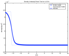
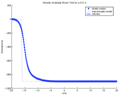
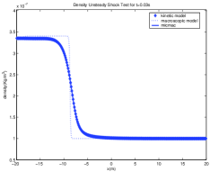
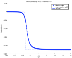
6.2 Unsteady Shock Tests

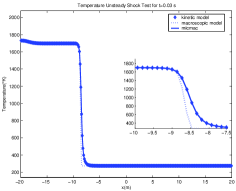
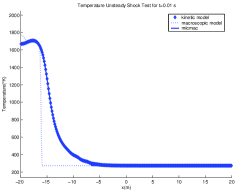
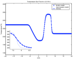
We consider an unsteady shock that propagates from left to right in the computational domain $x=-20\ m$, $x=20\ m$. The shock is produced pushing the hydrogen gas against a wall which is located on the left boundary. We consider that the particles are specularly reflected and that the wall instantaneously adopts the temperature of the gas. This effect is numerically simulated by setting macroscopic variables in ghost cells (two cells for a second order scheme) beyond the left boundary with parameters $\varrho,\ T$ equal to the values of the first cell while the momentum is set opposite. In the non equilibrium case $g_{K}$ is also different from zero in the ghost cell, and is equal to a specularly reflected copy of $g_{K}$ in the first cell. At the right boundary, we mimic the introduction of the gas by adding two ghost cells where, at each time step, the initial values for density, momentum and energy are fixed. The gas is supposed in thermodynamic equilibrium, which implies that $g_{K}=0$. The computation is stopped at the final time $t=0.04$ s. There are $300$ cells in physical space and $40$ cells in velocity space. We do not use a finer mesh because the scheme is second order. Symmetric artificial boundaries in velocity space are fixed at the beginning of the computation through the relation $v_{b}=\pm C_{1}\max(\sqrt{RT_{W}})$, where $R$ is the gas constant, $C_{1}$ is a parameter normally fixed equal to $4$ and $T_{W}$ is a temperature set equal to the maximum attainable temperature, which is obtained by supposing that all the kinetic energy is transformed into thermal energy. The transition function $h$ is initialized as $h=0$ (fluid region) everywhere.

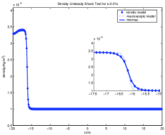
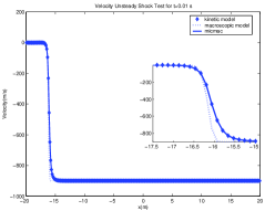
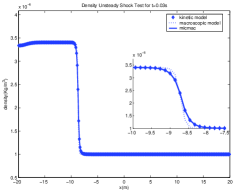
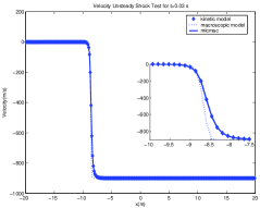
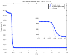
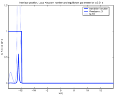
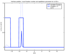
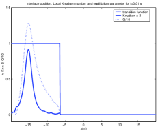
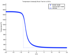
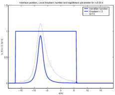
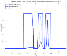
In the first test the initial conditions are $\varrho=10^{-6}$ kg/m³ for the mass density, $u=-900$ m/s for the mean velocity and $T=273$ K for the temperature. In Figure 1 we have reported the mass density on the left and the velocity on the right. ¿From top to bottom, time increases from $t=10^{-2}\ s$ (top) to $t=4\times 10^{-2}\ s$ (bottom), with $t=2\times 10^{-2}\ s$ middle top and $t=3\times 10^{-2}\ s$ middle bottom. In Figure 2 we have reported the temperature on the left, the transition function, the heat flux and the local Knudsen number on the right. From top to bottom the same instants of time as for the previous Figure are shown. In the plots regarding the macroscopic variables we reported the solution computed with our algorithm (mic-mac in the legend of the Figures), the solution computed with a kinetic solver and the solution computed with a macroscopic fluid solver. Magnifications of the solutions close to non equilibrium regions are given for clarity.

As soon as the simulation starts on the left boundary, the transition function $h$ increases from zero to one, which means that the solution is computed with the kinetic scheme, while in the rest of the domain the solution is still computed with the fluid scheme ($h=0$). When the shock starts to move towards the right, we notice a splitting of the kinetic region. One very narrow region still continues to follow the shock and one remains close to the left boundary. Once that the threshold values of the breakdown parameters $\beta$ and $\beta_{K}$ are fixed, the procedure automatically determines the sizes of the kinetic and buffer regions.

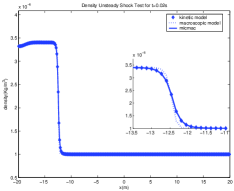
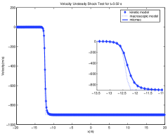
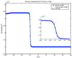
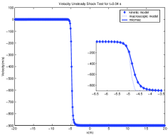
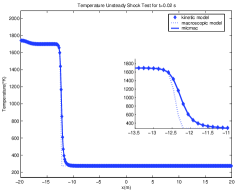
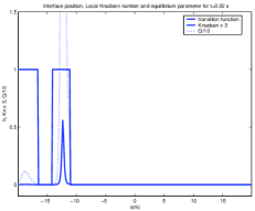
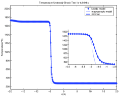
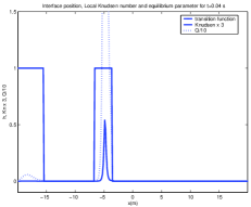
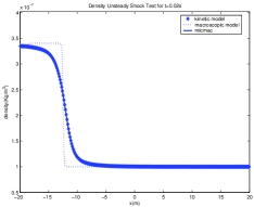
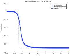
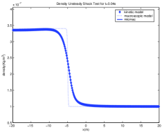
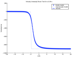
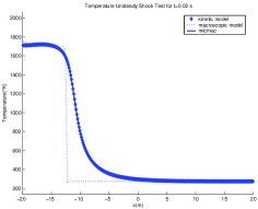
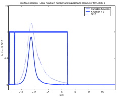
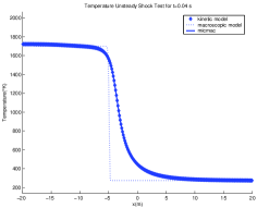
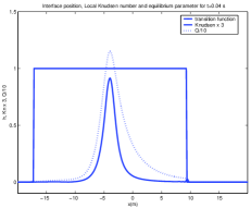
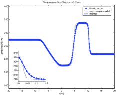
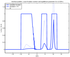
We repeat the simulation with a lower initial density $\varrho=10^{-7}$ kg/m³. This yields different results which are reported in Figure 3 for the density and velocity and in Figure 4 for the temperature, local Knudsen, heat flux and transition function. The results are obtained with the same criteria as in the previous test case. Again at the beginning $h$ is set equal to zero (fluid), but now the shock is much less sharp and the non equilibrium region becomes larger.

We observe that in this first test the discrepancy between the fully kinetic solver and the coupling strategy is not perceivable, while the computational time is reduced in proportion to the ratio between the areas of the kinetic and buffer regions compared to the entire domain. Thus, in the first case we have a reduction of approximately $70\%$ of the computational time while in the second one the reduction is only the $20\%$. Further reductions are possible through code optimization.

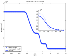
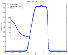
6.3 Sod Tests

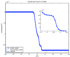
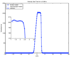
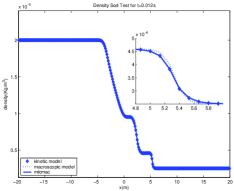
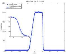
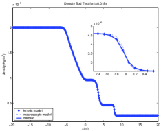
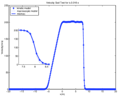
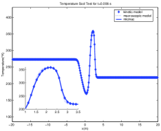
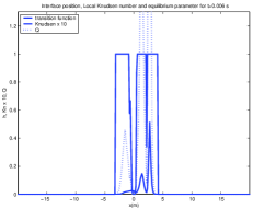
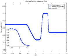
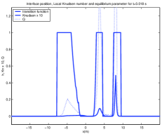
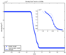
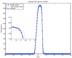
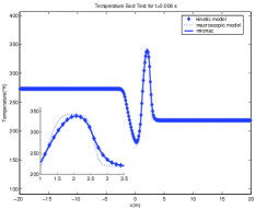
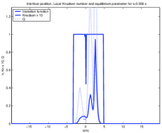
In these second series of tests, we consider the classical Sod initial data in a domain which ranges from $-20\ m$ to $20\ m$. The numerical parameters are the same as for the previous examples. Thus respectively $300$ and $40$ mesh points in physical and velocity space are used. Symmetric artificial boundary condition are fixed in velocity space at the same points $v_{b}=\pm C_{1}\max(\sqrt{RT_{W}})$, while Neumann boundary condition are chosen both for the kinetic (if necessary) and fluid models. Finally the simulations are initialized with a thermodynamic equilibrium with $h=0$ and $g_{K}=0$ everywhere.

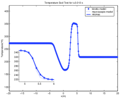
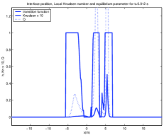
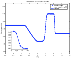
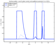
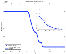
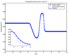
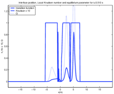
In the first case, we take the following initial conditions: mass density $\varrho_{L}=2\times 10^{-5}$ kg/m³, mean velocity $u_{L}=0$ m/s and temperature $T_{L}=273.15$ K if $-20\leq x\leq 0\ m$, while $\varrho_{R}=0.25\times 10^{-5}$ kg/m³, $u_{R}=0$ m/s, $T_{R}=218.4$ K if $0\leq x\leq 20\ m$. The results are reported in Figure 5 for the density (left) and velocity (right) and in Figure 6 for the temperature (left), Knudsen number, heat flux and transition function (right). Snapshot at increasing times are displayed top to down, corresponding successively to $t=6\times 10^{-3}\ s$, then $t=1.2\times 10^{-2}\ s$, $t=1.8\times 10^{-2}\ s$ and finally $t=2.4\times 10^{-2}\ s$. Again we provide magnifications of the solution close to non equilibrium zones in order to highlight the differences between the three different schemes: the macroscopic and kinetic ones and the coupling strategy (mic-mac in the legend). We observe that due to the initial shock, a kinetic region appears immediately and starts to grow in time, but as soon as the different non equilibrium regions separate, the kinetic region itself splits into three: one around the rarefaction wave, one around the contact discontinuity, and one around the shock. Even with magnifications it is not possible to perceive differences between the kinetic model and the coupling strategy, even though the kinetic regions remain very tiny, permitting a fast computation.

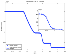
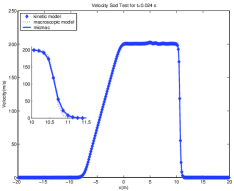
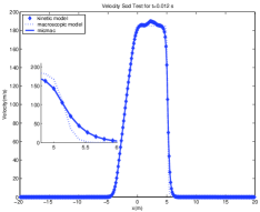
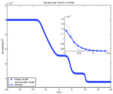
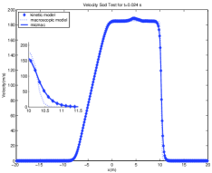
The simulation is repeated, with a lower initial density $\varrho_{L}=5\times 10^{-6}$ kg/m³ and $\varrho_{R}=0.75\times 10^{-6}$ kg/m³, and the results are displayed in Figure 7 for the density and velocity and in Figure 8 for the temperature, heat flux, local Knudsen and transition function. The same qualitative features as in the previous test can be observed, the only difference being that the kinetic regions are thicker, which means that the non equilibrium zone is larger. This is clearly visible from the plots of the macroscopic quantities: the difference between the kinetic and fluid models is significant in a large portion of the domain.

We finally observe that compared to [11], in which a similar scheme was developed, we are able to capture small discrepancies between the kinetic and macroscopic models in very tiny regions. This turns to be a much more efficient use of the domain decomposition technique. The computational time reduction is of the order of $70\%$ and $60\%$ respectively for the two tests compared to a kinetic solver.

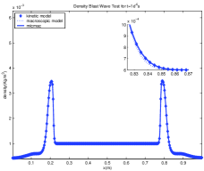
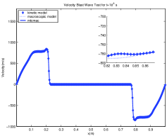
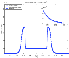
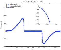
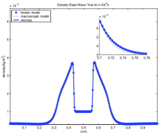
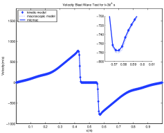
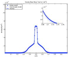
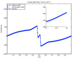
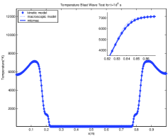
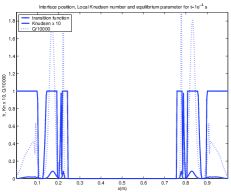
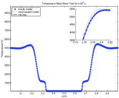
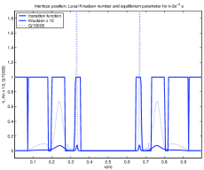
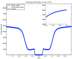
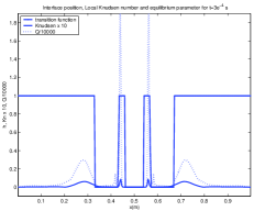
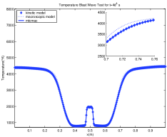
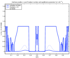
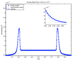
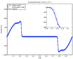
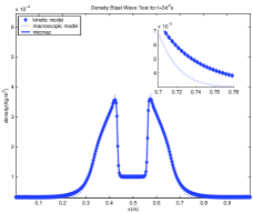
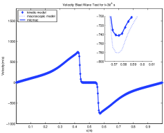
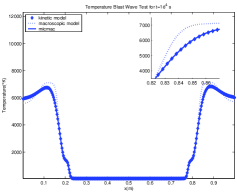
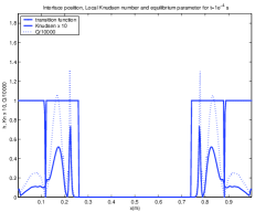
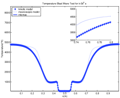
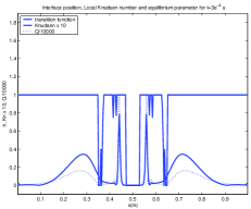
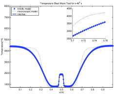
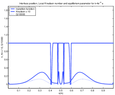
6.4 Blast Wave Tests

In this paragraph we present two interacting symmetric blast waves in hydrogen gas. The domain ranges from $x=0\ m$ to $x=1\ m$, while the numerical parameters in terms of mesh and velocity space boundaries are the same as in the previous tests. The physical boundaries are represented by two specularly reflecting walls, on which impinging particles are re-emitted in the opposite direction with the same velocity (in magnitude). Mass is conserved at the walls which additionally are supposed to adopt the gas temperature instantaneously. These effects are obtained like in the unsteady shock test with two ghost cells (four for a second order scheme), in which the same macroscopic values as those of the first and last cells are imposed, except for momentum which changes sign. The perturbation function $g_{K}$ can in general be different from zero and assumes the same values of its corresponding counterpart in the first and last cell, with a sign change in the velocity variable. At the beginning, we set $h=0$ and $g_{K}=0$ everywhere.

In the first test, the initial data are:

$$\varrho=10^{-3}kg/m^{3}\ \ u=200\ m/s\ \ T=10000\ K\ if\ x\leq 0.1$$

$$\varrho=10^{-3}kg/m^{3}\ \ u=-200\ m/s\ \ T=10000\ K\ if\ x\geq 0.9$$

$$\varrho=10^{-3}kg/m^{3}\ \ \ u=0\ m/s\ \ \ \ \ \ T=50\ K\ if\ 0.1\leq x\leq 0.9$$

The results in terms of the density and mean velocity are reported in Figure 9, while the temperature, local Knudsen, heat flux and transition function are reported in Figure 10. The displayed results are for increasing times $t=10^{-4}\ s$ to $t=4\times 10^{-4}\ s$ from top to bottom. Again we plot the kinetic, the fluid schemes and the coupling strategy (micmac scheme) in each Figure and magnifications close to non equilibrium regions are provided.

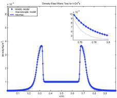
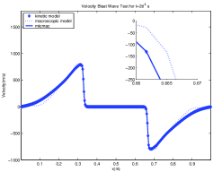
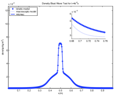
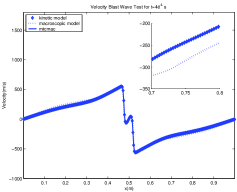
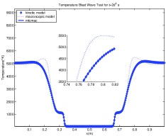
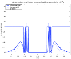
In the second test the initial density is decreased, and we use:

$$\varrho=10^{-4}kg/m^{3}\ \ u=200\ m/s\ \ T=10000\ K\ if\ x\leq 0.1$$

$$\varrho=10^{-4}kg/m^{3}\ \ u=-200\ m/s\ \ T=10000\ K\ if\ x\geq 0.9$$

$$\varrho=10^{-4}kg/m^{3}\ \ \ u=0\ m/s\ \ \ \ \ \ T=50\ K\ if\ 0.1\leq x\leq 0.9$$

The results obtained with this second set of data are reported in Figure 11 and 12. We observe that starting from a situation where the fluid model is used almost everywhere we end up in the opposite situation where the kinetic model is used in the whole domain($h=1\ \forall x$). Thus, while a static domain decomposition technique leads to similar computational times as a fully kinetic resolution, the coupling strategy leads to a speed up of about $40\%$ for the first test and $30\%$ for the second test, compared to a fully kinetic solver.

7 Conclusion

In this paper we have presented a moving domain decomposition method which provides an efficient way to deal with multiscale fluid dynamic problems. Regions far from thermodynamical equilibrium are treated with a kinetic solver. The method is based on the micro-macro decomposition technique developed by Degond-Liu-Mieussens [10] in which macroscopic fluid equations are coupled with a kinetic equation which describes the time evolution of the perturbation from equilibrium. The method consists in splitting the distribution function into an equilibrium part and a non-equilibrium part, together with the introduction of buffer zones and transition functions as proposed in [10], [8] and [11] to smoothly pass from the macroscopic model to the kinetic model and vice versa.

In order to build up an efficient method that can be used in a wide spectrum of situations, and by contrast to [10], we consider the possibility of moving the different domains like in [11], using however, a decomposition technique which shows enhanced performances. Moreover, we have developed a scheme which is able to automatically create, cancel and move as many kinetic, fluid or buffer regions as necessary. The method relies on the proper combination of the two equilibrium criteria we have identified and on a priori tolerance that we decide to accept. An important point also resides in the introduction of a new criterion for the breakdown of the fluid model, which is able to measure the discrepancy between the kinetic and the fluid model in a much more accurate way then the mere Knudsen number. Finally, we have proved that the coupling strategy preserves positivity under a CFL condition, and the uniform flows, also in the fully discrete case.

The last part of the work is devoted to several numerical tests. The results clearly demonstrate the advantages of this method over existing ones. The method captures the correct kinetic behaviors even in transition regions and provides significant improvements in terms of computational speedup while maintaining the accuracy of a kinetic solver.

In the future we will extend the method to make it consistent with the Navier-Stokes equations instead of the Euler model. This step can further improve the technique allowing very narrow kinetic zones and providing considerable speed-up while maintaining accuracy. We will also explore the use of Monte Carlo techniques for the full Boltzmann equation and that of time sub-cycling for the two models. We finally observe that the computational speed-up will significantly increase for two or three dimensional simulations, which we intend to carry out in the future. To conclude, because multiscale effects are very important also in many others fields we plan to extend our method to other models.

Appendix A Preservation of uniform flows

Preservation of uniform flows is a very important property, which prevents oscillations to appear when the transition region is located in a domain where the flow is smooth. In this appendix we compare the properties of the present micro-macro coupling strategy to those of the decomposition methods of [8, 9, 11] regarding preservation of uniform flows.

In [10], it has been demonstrated that the micro-macro model is able to preserve uniform flows in the continuous case. This property is also true for the decomposition used in [8, 9, 11], but only when the collision operator has specific properties (which are satisfied by the Boltzmann and BGK operator). In this appendix, we show that the present micro-macro coupling strategy is able to preserve uniform flows also in the discrete case independently of the choice of the discretization scheme. We observe that this property does not hold in the general case for the decompositions used in [8, 9, 11]. The satisfaction of this property by the present micro-macro coupling strategy constitutes a very big advantadge of this method over the previous ones [8, 9, 11].

As an example, we consider the decomposition used in [11], which reads

$$\frac{\partial\boldsymbol{\varrho}_{L}}{\partial t}+(1-h)\partial_{x}F(\boldsymbol{\varrho}_{L})+(1-h)\partial_{x}\langle vmf_{R}\rangle=-\boldsymbol{\varrho}\partial_{t}h$$ (55)

$$\partial_{t}f_{R}+hv\partial_{x}f_{R}+hv\partial_{x}E[\boldsymbol{\varrho}]=h\frac{\nu}{\varepsilon}(E[\boldsymbol{\varrho}]-f)+f\partial_{t}h,$$ (56)

where the distribution function is defined by $f=f_{R}+E[\boldsymbol{\varrho}_{L}]$, $f_{R}=hf$ and $E[\boldsymbol{\varrho}_{L}]=(1-h)E[\boldsymbol{\varrho}]$. In this model the solution of the full kinetic problem is given by $f_{R}$ if $x\in\Omega_{1}$, by $E[\boldsymbol{\varrho}_{L}]$ if $x\in\Omega_{2}$ and by $E[\boldsymbol{\varrho}_{L}]+f_{R}$ if $x\in\Omega_{3}$. This is due to the fact that $f_{R}=0$ for $x\in\Omega_{2}$, $E[\boldsymbol{\varrho}_{L}]=0$ for $x\in\Omega_{1}$, while in $\Omega_{3}$ they are both different from zero and the global solution is obtained as a sum of the two partial solutions. We refer to the above cited papers for details.

Here we recall that, in [8, 9, 11], small oscillations appear inside the transition regions except when the scheme used for the fluid part is an exact discrete velocity integration of the scheme used for the kinetic part (in this case, we say that the two schemes are ’compatible’, and are ’incompatible’ otherwise). These oscillations appear even in situations where preservation of uniform flows is true for the continuous model. To circumvent this problem, in [8, 9, 11], we used a standard shock-capturing scheme (such as e.g. the Godunov scheme) for the Euler equations in the pure fluid region (i.e. $h=0$), but we converted to a compatible scheme with the discretization of the kinetic model inside the buffer zones (see [11] for details). However, this choice introduces some implementation difficulties and reduces the performances. Indeed, a compatible scheme with the discretization of the kinetic model has intrinsically the same cost as the full kinetic solver, and the coupling strategy is twice more costly than the mere kinetic model in all the buffer region.

In order to prove the property that uniform flows are not preserved by the decomposition (55-56) in the discrete case, we focus on the first one of the two equations. The same considerations hold for the other one. If the initial data is such that $f=E[\boldsymbol{\varrho}]$ we have

$$\frac{\partial\boldsymbol{\varrho}_{L}}{\partial t}+(1-h)\partial_{x}F(\boldsymbol{\varrho}_{L})+(1-h)\partial_{x}\langle vmf_{R}\rangle+\boldsymbol{\varrho}\partial_{t}h=$$

$$=(1-h)\left(\frac{\partial\boldsymbol{\varrho}}{\partial t}+(1-h)\partial_{x}F(\boldsymbol{\varrho})+h\partial_{x}\langle vmE[\boldsymbol{\varrho}]\rangle-h^{\prime}F(\boldsymbol{\varrho})+h^{\prime}\langle vmE[\boldsymbol{\varrho}]\rangle\right)=$$

$$=(1-h)\left(\frac{\partial\boldsymbol{\varrho}}{\partial t}+(1-h)\partial_{x}F(\boldsymbol{\varrho})+h\partial_{x}\langle vmE[\boldsymbol{\varrho}]\rangle\right).$$

In the above equation, the time derivative with respect to $h$ disappears and so does the flux, using that $F(\boldsymbol{\varrho})=\langle vmE[\boldsymbol{\varrho}]\rangle$. In the continuous case it is also true that

$$(1-h)\partial_{x}F(\boldsymbol{\varrho})+h\partial_{x}\langle vmE[\boldsymbol{\varrho}]\rangle=\partial_{x}F(\boldsymbol{\varrho})=\partial_{x}\langle vmE[\boldsymbol{\varrho}]\rangle$$ (57)

and so, uniform flows are preserved. However, when we discretize the fluxes according to $\partial_{x}F(\boldsymbol{\varrho})=(\phi_{i+1/2}(\boldsymbol{\varrho})-\phi_{i-1/2}(\boldsymbol{\varrho}))/\Delta x$ and $\partial_{x}\langle vm{\cal E}(\boldsymbol{\varrho})\rangle=(\psi_{i+1/2}({\cal E}[\boldsymbol{\varrho}])-\psi_{i-1/2}({\cal E}[\boldsymbol{\varrho}]))/\Delta x$, the equality (57) does not hold anymore. In fact, in the general case we have

$$(1-h)\left(\frac{\phi_{i+1/2}(\boldsymbol{\varrho})-\phi_{i-1/2}(\boldsymbol{\varrho})}{\Delta x}\right)+h\left(\frac{\psi_{i+1/2}({\cal E}[\boldsymbol{\varrho}])-\psi_{i-1/2}({\cal E}[\boldsymbol{\varrho}])}{\Delta x}\right)\neq$$

$$\neq\left(\frac{\phi_{i+1/2}(\boldsymbol{\varrho})-\phi_{i-1/2}(\boldsymbol{\varrho})}{\Delta x}\right)\neq\left(\frac{\psi_{i+1/2}({\cal E}[\boldsymbol{\varrho}])-\psi_{i-1/2}({\cal E}[\boldsymbol{\varrho}])}{\Delta x}\right).$$

Thus, if two incompatible numerical schemes are used to discretize the kinetic and fluid fluxes, oscillations in the solution can appear as documented in [11]. However, we observe that, using the same numerical flux is not sufficient to ensure preservation of uniform flows through the decomposition (55-56). To that aim, consider a generic discretization of the coupled system (55-56):

$$\boldsymbol{\varrho}^{n+1}_{i,L} =\boldsymbol{\varrho}^{n}_{i,L}-(1-h_{i})\frac{\Delta t}{\Delta x}\left(\psi_{i+1/2}(\boldsymbol{\varrho}_{L}^{n})-\psi_{i-1/2}(\boldsymbol{\varrho}_{L}^{n})\right)$$

$$-(1-h_{i})\frac{\Delta t}{\Delta x}\sum_{k}\mathbf{m}_{k}\left(\psi_{i+1/2}(f_{k,R}^{n})-\psi_{i-1/2}(f_{k,R}^{n})\right)\Delta v,$$ (58)

$$f^{n+1}_{k,i,R}=f_{k,i,R}^{n} -h_{i}\frac{\Delta t}{\Delta x}\left(\phi_{i+1/2}(f^{n}_{k,R})-\phi_{i-1/2}(f^{n}_{k,R})\right)$$

$$-h_{i}\frac{\Delta t}{\Delta x}\left(\phi_{i+1/2}({\cal E}_{k}[\boldsymbol{\varrho}^{n}_{L}])-\phi_{i-1/2}({\cal E}_{k}[\boldsymbol{\varrho}^{n}_{L}])\right)$$ (59)

$$+h_{i}\frac{\Delta t\nu}{\varepsilon}\left({\cal E}_{k}[\boldsymbol{\varrho}^{n}_{i}]-f^{n}_{k,i}\right),$$

where a discrete velocity model has been used to resolve the kinetic equation (59) with $\mathbf{m}_{k}$ the discretized collision invariants. The function $\phi_{i\pm 1/2},\psi_{i\pm 1/2}$ are two different generic numerical fluxes while, for simplicity, the function $h$ is considered constant in time. The initial data are $\boldsymbol{\varrho}^{0}_{i}=\boldsymbol{\varrho}_{0}$, $f^{0}_{i}=E[\boldsymbol{\varrho}_{0}]$, $f^{0}_{R,i}=h_{i}f_{0}$, $\boldsymbol{\varrho}^{0}_{L,i}=(1-h_{i})\boldsymbol{\varrho}_{0}$ and $E[\boldsymbol{\varrho}^{0}_{L,i}]=(1-h_{i})E[\boldsymbol{\varrho}_{0}]$ $\forall i$. Now, supposing the flow uniform at time $n$ we will see that not every numerical scheme ensures a uniform flow at time $n+1$. To this aim, if we integrate equation (59) multiplied by the collision invariants $\textbf{m}_{k}$ over the velocity space, we can rewrite the coupled numerical schemes (58-59) as follows:

$$\boldsymbol{\varrho}^{n+1}_{i,L}=\sum_{j=i}^{i\pm I}\boldsymbol{A}_{j}\boldsymbol{\varrho}^{n}_{j,L},$$ (60)

$$\boldsymbol{\varrho}^{n+1}_{i,R}=\sum_{j=i}^{i\pm I1}\sum_{k}^{K}\boldsymbol{B}_{j,k}\mathbf{m}_{k}f^{n}_{j,R}\Delta v,$$ (61)

with $\boldsymbol{\varrho}^{n+1}_{j,R}=\sum_{k}\mathbf{m}_{k}f^{n+1}_{j,R}\Delta v$, $I$ and $I1$ the length of the stencils in physical space and $K$ in velocity space. The symbols $\boldsymbol{A}_{j}$ and $\boldsymbol{B}_{j,k}$ represent the weights determined by the particular choice of the numerical schemes. Without loss of generality, suppose that $I=I1$. Then, we have that

$$\boldsymbol{\varrho}^{n+1}_{i} = \boldsymbol{\varrho}^{n+1}_{i,L}+\boldsymbol{\varrho}^{n+1}_{i,R}=\sum_{j}\boldsymbol{A}_{j}\boldsymbol{\varrho}^{n}_{j,L}+\sum_{j}\sum_{k}\boldsymbol{B}_{j,k}\mathbf{m}_{k}f^{n}_{j,R}\Delta v=$$ (62)

$$=\sum_{j}\boldsymbol{A}_{j}(\boldsymbol{\varrho}^{n}_{j,L}+\boldsymbol{\varrho}^{n}_{j,R})+\sum_{j}\left[\left(\sum_{k}\boldsymbol{B}_{j,k}\mathbf{m}_{k}f^{n}_{j,R}\right)-\boldsymbol{A}_{j}\boldsymbol{\varrho}^{n}_{j,R}\right]=$$

$$=\sum_{j}\boldsymbol{A}_{j}\boldsymbol{\varrho}^{n}_{j}+\sum_{j}\left[\left(\sum_{k}\boldsymbol{B}_{j,k}\mathbf{m}_{k}f^{n}_{j,R}\right)-\boldsymbol{A}_{j}\boldsymbol{\varrho}^{n}_{j,R}\right]=$$

$$=\boldsymbol{\varrho}^{n}_{i}+\sum_{j}\left[\left(\sum_{k}\boldsymbol{B}_{j,k}\mathbf{m}_{k}f^{n}_{j,R}\right)-\boldsymbol{A}_{j}\boldsymbol{\varrho}^{n}_{j,R}\right]$$

which means that we do not have preservation of uniform flows except in some particular cases, such as, for instance, when the numerical schemes used to discretize the two equations (58-59) are compatible. Therefore, such compatible schemes are needed in all buffer zones to make sure that oscillations in the solutions will be avoided.

Instead if we consider the present micro-macro coupling strategy with the same initial data $f=E[\boldsymbol{\varrho}]$, the following property holds:

Proposition 2.

If the initial condition $f^{0}\geq 0$ is a constant equilibrium $E[\boldsymbol{\varrho}^{0}]$, then $\boldsymbol{\varrho}=\boldsymbol{\varrho}^{0}$ and $g_{K}=h(f-E[\boldsymbol{\varrho}])=0$ are solutions of the micro-macro model (23-24), and $E[\boldsymbol{\varrho}]+g_{K}=E[\boldsymbol{\varrho}^{0}]$. In other words, the kinetic/fluid solution of the micro-macro model is exactly the solution of the original kinetic model.

Indeed, for the micro-macro decomposition, the total flux is independent of $h$ in equilibrium regimes and is not obtained as a sum of two complementary terms weighted by the function $h$. It follows directly that the micro-macro method preserves uniform flows even in the discrete case independently of the choice of the numerical scheme.

Figure 1: Unsteady Shock 1: Solution at $t=1\times 10^{-2}$ top, $t=2\times 10^{-2}$ middle top, $t=3\times 10^{-2}$ middle bottom, $t=4\times 10^{-2}$ bottom, density left, velocity right. The small panels are a magnification of the solution close to the shock.

Figure 2: Unsteady Shock 1: Solution at $t=1\times 10^{-2}$ top, $t=2\times 10^{-2}$ middle top, $t=3\times 10^{-2}$ middle bottom, $t=4\times 10^{-2}$ bottom, temperature left, transition function, Knudsen number and heat flux right. The small panels are a magnification of the solution close to the shock.

Figure 3: Unsteady Shock 2: Solution at $t=1\times 10^{-2}$ top, $t=2\times 10^{-2}$ middle top, $t=3\times 10^{-2}$ middle bottom, $t=4\times 10^{-2}$ bottom, density left, velocity right.

Figure 4: Unsteady Shock 2: Solution at $t=1\times 10^{-2}$ top, $t=2\times 10^{-2}$ middle top, $t=3\times 10^{-2}$ middle bottom, $t=4\times 10^{-2}$ bottom, temperature left, transition function, Knudsen number and heat flux right.

Figure 5: Sod Test 1: Solution at $t=0.6\times 10^{-2}$ top, $t=1.2\times 10^{-2}$ middle top, $t=1.8\times 10^{-2}$ middle bottom, $t=2.4\times 10^{-2}$ bottom, density left, velocity right. The small panels are a magnification of the solution close to non equilibrium regions.

Figure 6: Sod Test 1: Solution at $t=0.6\times 10^{-2}$ top, $t=1.2\times 10^{-2}$ middle top, $t=1.8\times 10^{-2}$ middle bottom, $t=2.4\times 10^{-2}$ bottom, temperature left, transition function , Knudsen number and heat flux right. The small panels are a magnification of the solution close to non equilibrium regions.

Figure 7: Sod Test 2: Solution at $t=0.6\times 10^{-2}$ top, $t=1.2\times 10^{-2}$ middle top, $t=1.8\times 10^{-2}$ middle bottom, $t=2.4\times 10^{-2}$ bottom, density left, velocity right. The small panels are a magnification of the solution close to non equilibrium regions.

Figure 8: Sod Test 2: Solution at $t=0.6\times 10^{-2}$ top, $t=1.2\times 10^{-2}$ middle top, $t=1.8\times 10^{-2}$ middle bottom, $t=2.4\times 10^{-2}$ bottom, temperature left, transition function, Knudsen number and heat flux right. The small panels are a magnification of the solution close to non equilibrium regions.

Figure 9: Blast Wave Test 1: Solution at $t=1\times 10^{-4}$ top, $t=2\times 10^{-4}$ middle top, $t=3\times 10^{-4}$ middle bottom, $t=4\times 10^{-4}$ bottom, density left, velocity right. The small panels are a magnification of the solution close to non equilibrium regions.

Figure 10: Blast Wave Test 1: Solution at $t=1\times 10^{-4}$ top, $t=2\times 10^{-4}$ middle top, $t=3\times 10^{-4}$ middle bottom, $t=4\times 10^{-4}$ bottom, temperature left, transition function, Knudsen number and heat flux right. The small panels are a magnification of the solution close to non equilibrium regions.

Figure 11: Blast Wave Test 2: Solution at $t=1\times 10^{-4}$ top, $t=2\times 10^{-4}$ middle top, $t=3\times 10^{-4}$ middle bottom, $t=4\times 10^{-4}$ bottom, density left, velocity right.

Figure 12: Blast Wave Test 2: Solution at $t=1\times 10^{-4}$ top, $t=2\times 10^{-4}$ middle top, $t=3\times 10^{-4}$ middle bottom, $t=4\times 10^{-4}$ bottom, temperature left, transition function, Knudsen number and heat flux.

References

- [1] O. Aktas, and N.R. Aluru, A combined continuum/DSMC technique for multiscale analysis of microfluidic filters. J. Comp. Phys., vol.178, (2002) pp. 342–72.
- [2] G. A. Bird, Molecular gas dynamics and direct simulation of gas flows, Clarendon Press, Oxford (1994).
- [3] J. F. Bourgat, P. LeTallec, B. Perthame, and Y. Qiu, Coupling Boltzmann and Euler equations without overlapping, in Domain Decomposition Methods in Science and Engineering, Contemp. Math. 157, AMS, Providence, RI, (1994), pp. 377–398.
- [4] J. F. Bourgat, P. LeTallec, M.D. Tidriri, Coupling Boltzmann and Navier-Stokes equations by friction. J. Comput. Phys. 127, 2, (1996), pag. 227–245.
- [5] C. Cercignani, The Boltzmann Equation and Its Applications, Springer-Verlag, New York, (1988).
- [6] G. Q. Chen, D. Levermore and T. P. Liu, Hyperbolic conservation laws with stiff relaxation terms and entropy, Comm. Pure Appl. Math., 47 (1994), pp. 787–830.
- [7] N. Crouseilles, P. Degond, M. Lemou, A hybrid kinetic-fluid model for solving the gas-dynamics Boltzmann BGK equation, J. Comp. Phys., 199 (2004) 776-808.
- [8] P. Degond, S. Jin, L. Mieussens, A Smooth Transition Between Kinetic and Hydrodynamic Equations , J. Comp. Phys., 209 (2005) 665–694.
- [9] P. Degond and S. Jin, A Smooth Transition Between Kinetic and Diffusion Equations, SIAM J. Numer. Anal., 2005, vol. 42, no6, pp. 2671-2687 .
- [10] P. Degond, J.G. Liu, L. Mieussens, Macroscopic Fluid Model with Localized Kinetic Upscaling Effects, SIAM Multi. Model. Sim. 5(3), 940–979 (2006)
- [11] P.Degond, G. Dimarco, L. Mieussens., A Moving Interface Method for Dynamic Kinetic-fluid Coupling. J. Comp. Phys., Vol. 227, pp. 1176-1208, (2007).
- [12] G. Dimarco and L. Pareschi, A Fluid Solver Independent Hybrid Method for Multiscale Kinetic equations., Submitted to SIAM J. Sci. Comp.
- [13] G. Dimarco and L. Pareschi, Domain Decomposition Techniques and Hybrid Multiscale Methods for kinetic equations, Proceedings of the 11th International Conference on Hyperbolic problems: Theory, Numerics, Applications, pp. 457-464 (2007).
- [14] W. E and B. Engquist, The heterogeneous multiscale methods, Comm. Math. Sci., 1, (2003), pp. 87-133.
- [15] H.S. Wijesinghe, N.G. Hadjiconstantinou, Discussion of Hybrid Atomistic-Continuum Methods for Multiscale Hydrodynamics. Int. J. Multi. Comp. Eng., Vol.2 pp. 189 202(2004).
- [16] A. B. Huang and P. F. Hwang, Test of statistical models for gases with and without internal energy states, Phy. Fluids, 16(4):466 475, 1973.
- [17] S. Jin and Z. P. Xin, Relaxation schemes for systems of conservation laws in arbitrary space dimensions, Comm. Pure Appl. Math., 48 (1995), pp. 235–276.
- [18] A. Klar and C. Schmeiser, Numerical passage from radiative heat transfer to nonlinear diffusion models, Math. Models Methods Appl. Sci., Vol. 11, pp.749- 767, 2001.
- [19] V.I. Kolobov, R.R. Arslanbekov,V.V. Aristov, A.A. Frolova, S.A. Zabelok, Unified Solver for Rarefied and Continuum Flows with Adaptive Mesh and Algorithm Refinement, J. Comp. Phys., Vol. 223 No. 2, pp. 589–608 (2007).
- [20] D. Levermore, W.J.Morokoff, B.T. Nadiga, Moment realizability and the validity of the Navier Stokes equations for rarefied gas dynamics, Phy. Fluids, Vol. 10, No. 12, (1998).
- [21] L. Mieussens, Discrete Velocity Model and Implicit Scheme for the BGK Equation of Rarefied Gas Dynamic, Math. Models Meth. App. Sci., Vol 10 No. 8 (2000) 1121-1149.
- [22] L. Mieussens, Convergence of a discrete-velocity model for the Boltzmann-BGK equation, Comput. Math. Appl., 41(1-2):83–96, 2001.
- [23] P. LeTallec and F. Mallinger, Coupling Boltzmann and Navier-Stokes by half fluxes J. Comp. Phys., 136, (1997) pp. 51–67.
- [24] R. J. LeVeque, Numerical Methods for Conservation Laws, Lectures in Mathematics, Birkhauser Verlag, Basel (1992).
- [25] Z.-H. Li and H.-X. Zhang, Numerical investigation from rarefied flow to continuum by solving the Boltzmann model equation, Int. J. Num. Meth. Fluids, Vol. 42, 4, (2003) pp. 361–382.
- [26] J.C. Mandal, and S.M. Deshpande, Kinetic flux vector splitting for Euler equations, Comp. Fluids, Vol.23, (1994), pp. 447–78.
- [27] R. Roveda, D.B. Goldstein, and P.L. Varghese, Hybrid Euler/Particle Approach for Continuum/ Rarefied Flows, AIAA J. Spacecraft Rockets 35, (1998), pp. 258–265.
- [28] T. Schulze, P. Smereka and W. E, Coupling kinetic Monte-Carlo and continuum models with application to epitaxial growth, J. Comput. Phys., 189, (2003), pp. 197–211.
- [29] Q. Sun, I. D. Boyd, G.V. Candler, A hybrid continuum/particle approach for modeling subsonic, rarefied gas flows. J. Comp. Phys., 194 (2004) 256 277.
- [30] S. Tiwari, Coupling of the Boltzmann and Euler equations with automatic domain decomposition, J. Comput. Phys., vol. 144, 1998, 710–726.
- [31] S. Tiwari, Application Of moment realizability criteria for coupling of the Boltzmann and the Euler equations, Transp. Theory Stat. Phys., Vol. 29, 7 pp 759–783
- [32] W.-L. Wang and I. D. Boyd, Predicting Continuum breakdown in Hypersonic Viscous Flows, Phys. Fluids, Vol. 15, 2003, pp 91-100.
- [33] D.C. Wadsworth, D.A. Erwin Two dimensional hybrid continuum/particle simulation approach for rarefied hypersonic flows. AIAA Paper 92-2975, 1992.
- [34] H.S. Wijesinghe, R.D. Hornung, A. L. Garcia, N. G. Hadjiconstantinou, Three dimensional hybrid continuum-atomistic simulations for multiscale hydrodynamics. J. Fluids Eng. (to appear).