Dynamical systems analysis of stack filters

Abstract

We study classes of dynamical systems that can be obtained by constructing recursive networks with monotone Boolean functions. Stack filters in nonlinear signal processing are special cases of such systems. We show an analytical connection between coefficients used to optimize the statistical properties of stack filters and their sensitivity, a measure that can be used to characterize the dynamical properties of Boolean networks constructed from the corresponding monotone functions. A connection is made between the rank selection probabilities (RSPs) and the sensitivity. We also examine the dynamical behavior of monotone functions corresponding to filters that are optimal in terms of their noise suppression capability, and find that the optimal filters are dynamically chaotic. This contrasts with the optimal information preservation properties of critical networks in the case of small perturbations in Boolean networks, and highlights the difference between such perturbations and those corresponding to noise. We also consider a generalization of Boolean networks that is obtained by utilizing stack filters on continuous-valued states. It can be seen that for such networks, the dynamical regime can be changed when binary variables are made continuous.

1 Introduction

Biological systems can be viewed as dynamical systems of biomolecular interactions that process information from their environment and mount diverse, yet specific responses, striking a balance between stability and adaptability. Living systems need to remain stable under variable environmental conditions and yet be able to evolve and respond to specific stimuli. This trade-off between adaptability and stability can be captured, in the context of dynamical systems analysis, by an order parameter that quantifies the sensitivity of the system to perturbations, such as environmental and molecular noise.

Recent experimental evidence has been mounting in support of a long-standing hypothesis stating that living systems operate at the critical regime between ordered and disordered behavior [1, 2, 3, 4]. Furthermore, critical systems have been shown to be optimal in several ways. For example, they are able to store a maximal amount of information [5] and propagate the information with minimal information loss in a noisy environment [6]. Additionally, critical systems exhibit the most complex relationships between their structure and dynamics [7]. Thus, optimality of a dynamical system can be considered as a trade-off between noise suppression and detail preservation. Such a trade-off is also the central goal of designing digital filters in signal processing. Indeed, digital filters can be studied in the context of dynamical systems theory [8].

In this contribution, we consider the well known class of nonlinear digital filters, called stack filters. There exists a well established statistical theory for the optimization of stack filters for a given noise distribution [9, 10]. Statistical properties of stack filters can be represented by a set of coefficients and these can be used to design an optimal class of stack filters that minimizes some statistical criterion, such as noise variance at the output of the filter [11, 12]. These coefficients can also be used to derive statistics that quantify the properties of the filters. Since the output of a stack filter is always one of the inputs, rank selection probabilities (RSP) quantify robustness and the noise suppression of the filter, specifying the probability that a sample of a particular rank in the input window will be used as the output of the filter; while sample selection probabilities (SSP) can be used to study the filter’s detail preservation, specifying the probability that a particular sample in the input window appears at the output [13]. Thus, these statistics capture the trade-off between robustness and detail preservation. For example, the median filter is extremely robust, but preserves details rather poorly, since its RSPs are all zero, except the center one, which is equal to one (the one corresponding to the median), while the SSPs are all equal (i.e., the uniform distribution). At the other extreme, the identity filter has the highest level of detail preservation, but very poor robustness to noise, since the RSPs are all equal, while the SSPs are all zero, except for the center one, which is equal to one (the one corresponding to the center position of the window).

We will show an analytical relationship between stack filter coefficients, rank selection properties, and the order parameter (essentially, Lyapunov exponent) that characterizes the behavior of the corresponding dynamical system, thus connecting the statistical optimization of stack filters with dynamical systems theory.

2 Background

2.1 Boolean networks and dynamical regimes

A Boolean network model is a conceptually simple dynamical system model where each node can be in only two possible states, on or off. Despite the apparent simplicity, this model class is able to produce highly complex behavior, for example, in the form of a phase transition between two dynamical regimes in which small perturbations are either attenuated or amplified. A Boolean network model can be defined as follows.

Let $s_{i}(t)\in\{0,1\}$, $i=1,\ldots,N$, where $N$ is the number of nodes in the network, be the state of $i$th node in the Boolean network at time $t$. The state of this node at time $t+1$ is determined by the states of nodes $j_{1},j_{2},{\ldots},j_{k_{i}}$ at time $t$ as

$$s_{i}(t+1)=f_{i}(s_{j_{1}}(t),s_{j_{2}}(t),{\ldots},s_{j_{k_{i}}}(t)),$$ (1)

where $f_{i}:\{0,1\}^{k_{i}}\rightarrow\{0,1\}$ is a Boolean function of $k_{i}$ variables. A binary vector $s\left(t\right)=\left(s_{1}\left(t\right),\ldots,s_{N}\left(t\right)\right)$ is said to be the state of the network at time $t.$ In the classical model, all nodes are updated synchronously as the system transitions from state $s\left(t\right)$ to state $s\left(t+1\right)$ [1]. The state transitions are determined by the multi-output Boolean function $F=(f_{1},{\ldots},f_{N})$ as $s(t+1)=F(s(t)),$ where $f_{i}$ is the Boolean function of node $i$ with predetermined connections from the nodes $j_{1},j_{2},{\ldots},j_{k_{i}}.$ It should be noted that this model can directly be generalized to a larger alphabet by defining $s_{i}(t)\in\{0,\ldots,L-1\}$ and $f_{i}:\{0,\ldots,L-1\}^{k_{i}}\rightarrow\{0,\ldots,L-1\}$, where $L$ is the size of the alphabet. We restrict our attention to the case $L=2.$

To construct a Boolean network, the inputs $j_{1},j_{2},{\ldots},j_{k_{i}}$ for each node $i$ needs to be determined. This can be done by selecting the inputs randomly among all $N$ nodes or by selecting the inputs using some systematic pattern. The number of inputs $k_{i}$ can be endowed with a probability distribution, such as the power-law [14, 15] or Poisson distribution, with a mean $K=E\left[k_{i}\right],$ known as the average connectivity of the network.

Once the connections have been set, we can choose a Boolean function $f_{i}$ for each node. Functions can be parameterized by the bias $b=E\left[f_{i}\right]$, the probability that the function outputs one on an arbitrary input vector. If $b=0.5$, then the function is said to be unbiased. The functions can be selected randomly among all $2^{2^{k_{i}}}$ Boolean functions or they can be selected from some class of functions [16, 17, 18, 19]. If both the functions and connections are selected randomly, then the obtained network is called a random Boolean network (RBN) [1].

Since a Boolean network is a discrete system, it has a finite state space. Thus, every state trajectory, that is, a path through the state space from any initial state, will eventually return to one of the previously visited states. This kind of a state cycle where the same states are repeated infinitely is known as an attractor cycle and the states within the cycle are called attractor states. A set of states that leads to the same attractor is called the basin of attraction [20].

Boolean networks, as models of dynamical systems, can operate in the ordered or chaotic regimes, or at the phase transition boundary between these two regimes [21]. This phase transition regime has been referred to as the edge of chaos [1]. When a network is operating in the ordered regime, it is intrinsically robust while its dynamical behavior is simple. The robustness can be observed through both the structural and transient perturbations. Perturbations have a small effect on the behavior of the network. Networks in the chaotic regime, on the other hand, are extremely sensitive to perturbations. Even a small perturbation will quickly propagate through the entire network. Thus, networks in the chaotic regime are not robust in that they are not able to coordinate macroscopic behavior under perturbations. A phase transition between the ordered and chaotic regimes represents a trade-off between the need for stability and the need to have a wide range of dynamical behavior to respond to variable perturbations [1].

By varying the parameters $K$ and $b$ in the random Boolean network model, a dynamical phase transition can take place. The average sensitivity of the Boolean network

$$\sigma=2b(1-b)K$$ (2)

can be used to determine the dynamical regime. If $\sigma>1$ then the system is chaotic and for $\sigma<1$ the system is ordered [22, 23, 24, 25]. It is easy to see that for unbiased random Boolean networks, the critical connectivity is $K_{c}=2$.

In a sense, critical systems are maximally responsive to the useful information in their environment while being able to reliably execute their behaviors in the presence of uninformative variation in this environment. A hallmark of critical behavior is the spontaneous emergence of complex and coordinated macroscopic behavior in the form of long-range spatial or temporal correlations. Such coordination across many scales enables information to propagate over time from one part of the system to another with a high degree of specificity and sensitivity. These aspects of criticality support the idea that living cells, as complex dynamical systems of interacting biomolecules, are dynamically critical systems.

2.2 Stack Filters

Stack filters constitute an important class of nonlinear filters based on monotone Boolean functions [26]. Statistical properties of stack filters have been studied in terms of output distributions and moments for independent and identically distributed input signals [27, 11]. Consequently, it becomes possible to optimize stack filters in the mean square sense. In other words, the knowledge of the input distribution allows one to find a stack filter or a set of stack filters that minimize the output variance.

Rank selection probabilities (RSP) and sample selection probabilities (SSP) are probabilities that the output equals a sample with a certain rank and certain time-index in the filter window, respectively. The output distribution of a stack filter can be expressed in terms of its RSP’s. On the other hand, SSP’s give us information about the temporal behavior of stack filters. This information is important for examining the detail preservation properties of stack filters.

Let $\alpha=\left(\alpha_{1},\cdots,\alpha_{n}\right)$ and $\beta=\left(\beta_{1},\cdots,\beta_{n}\right)$ be two different $n$-element binary vectors. We say that $\alpha$ precedes $\beta$, denoted as $\alpha\prec\beta$, if $\alpha_{i}\leq\beta_{i}$ for every $i$, $1\leq i\leq n$. If $\alpha\nprec\beta$ and $\beta\nprec\alpha$, then $\alpha$ and $\beta$ are said to be incomparable. Relative to the predicate $\prec$, the set of all binary vectors of a given length is a partially ordered set. A Boolean function $f\left(x_{1},\cdots,x_{n}\right)$ is called monotone if for any two vectors $\alpha$ and $\beta$ such that $\alpha\prec\beta$, we have $f\left(\alpha\right)\leq f(\beta)$. The class of monotone Boolean functions is one of the most widely used and studied classes of Boolean functions.

Let $E^{n}$ denote the Boolean $n$-cube, that is, a graph with $2^{n}$ vertices each of which is labeled by an $n$-element binary vector. Two vertices $\alpha=\left(\alpha_{1},\cdots,\alpha_{n}\right)$ and $\beta=\left(\beta_{1},\cdots,\beta_{n}\right)$ are connected by an edge if and only if the Hamming distance $\rho(\alpha,\beta)=\sum_{i=1}^{n}\left(\alpha_{i}\oplus\beta_{i}\right)=1,$ where $\oplus$ is addition modulo 2 (exclusive OR). The set of those vectors from $E^{n}$ in which there are exactly $k$ units, $0\leq k\leq n$, is called the $k$th layer of $E^{n}$ and is denoted by $E^{n,k}$. The Hamming weight of the vector $x\in\{0,1\}^{n}$ is $w(x)=\rho(x,0),$ where $0$ is the all-zero vector.

A stack filter is defined by a monotone Boolean function. A continuous stack filter $S_{f}(\cdot)$, based on function $f$, is obtained by replacing conjunction $(\cdot)$ and disjunction $(+)$ operations by $\min(\cdot)$ and $\max(\cdot)$ operations, respectively. For example, the monotone Boolean function $f(x_{1},x_{2},x_{3})=x_{2}+x_{1}x_{3}$ corresponds to the continuous stack filter $S_{f}(X_{1},X_{2},X_{3})=\max(X_{2},\min(X_{1},X_{3})).$

Suppose that the input variables of some stack filter $S_{f}(\cdot)$ are i.i.d. random variables with distribution $F(t)=\Pr\{X_{i}\leq t\}$. Then, it is well known [27] that the output $Y=S_{f}(X_{1},{\ldots},X_{n})$ of the stack filter has output distribution

$$\Phi(t)=\sum_{i=0}^{n-1}A_{i}(1-F(t))^{i}F(t)^{n-i}$$ (3)

where

$$A_{i}=|\{x\in E^{n,i}:f(x)=0\}|.$$ (4)

It is known [28, 29] that rank selection probabilities $p_{i}=\Pr\{Y=X_{(i)}\},$ where $X_{(i)}$ is the $i$th order statistic, are obtained as,

$$p_{i}=\frac{A_{n-i}}{{\binom{n}{n-i}}}-\frac{A_{n-i+1}}{{\binom{n}{n-i+1}}}.$$ (5)

It can also be shown that the output distribution function of the filter can be expressed in terms of the RSPs as

$$\Phi(t)=\sum_{i=1}^{n}p_{i}F_{(i)}(t),$$ (6)

where $F_{(i)}(t)$ is the cumulative distribution function of the $i$th-order statistic for i.i.d. inputs [9].

Let $s_{j}=\Pr\{Y=X_{j}\}$ be the $j$th SSP and $s=(s_{1},{\ldots},s_{n})$ be the vector of SSPs. In [30], it was shown that $s_{j}=d_{j}(1)-d_{j}(0)$, where

$$d_{j}(k)=\sum_{x\in f^{-1}(1)|x_{j}=k}\left[n{\binom{{n-1}}{{w(x)-k}}}\right]^{-1}$$ (7)

and $f^{-1}(k)=\{x\in E^{n}:f(x)=k\}$.

For a given input distribution, the mean square optimization of stack filters can be performed as follows. The variance $\mu_{2}=E\{(Y-E\{Y\})^{2}\}$ of the output $Y$ of the stack filter can be written as

$$\mu_{2}=\sum_{i=0}^{n-1}A_{i}M(F,2,n,i)-\left(\sum_{i=0}^{n-1}A_{i}M(F,1,n,i)\right)^{2},$$ (8)

where

$$M(F,k,n,i)=\int_{-\infty}^{\infty}x^{k}\frac{d}{dt}((1-F(t))^{i}F(t)^{n-i})dx.$$ (9)

Thus, for a given noise distribution, the goal of optimization is to find parameters $A_{i}$ (equivalently, the rank selection probabilities) such that the objective function (8) is minimized. An optimal stack filter, specified by monotone Boolean function $f$, is then constructed using the obtained parameters $A_{i}$. As a result of optimization, we obtain a set of parameters $A_{i}$ that define a class of stack filters. In a given class, all stack filters are statistically equivalent since they all possess the same parameters $A_{i}$. Thus, they will also have the same rank selection probabilities $p_{i}$. An approach to select the best filter, in terms of its ability to preserve details, from the class of such statistically equivalent optimal stack filters has been proposed in [13].

2.3 Average sensitivity of Boolean functions

Let $f:\left\{0,1\right\}^{n}\rightarrow\left\{0,1\right\}$ be a Boolean function of $n$ variables $x_{1},\ldots,x_{n}$. Let

$$\partial f\left(x\right)/\partial x_{j}=f\left(x^{\left(j,0\right)}\right)\oplus f\left(x^{\left(j,1\right)}\right)$$ (10)

be the partial derivative of $f$ with respect to $x_{j}$, where $x^{\left(j,k\right)}=\left(x_{1},\ldots,x_{j-1},k,x_{j+1},\ldots x_{n}\right)$, $\,k=0,1$. Clearly, the partial derivative is a Boolean function itself that specifies whether a change in the $j$th input causes a change in the original function $f$. Now, the activity of variable $x_{j}$ in function $f$ can be defined as

$$\alpha_{j}^{f}=\frac{1}{2^{n}}\sum_{x\in\left\{0,1\right\}^{n}}\partial f\left(x\right)/\partial x_{j}.$$ (11)

Note that although the vector $x$ consists of $n$ components (variables), the $j$th variable is fictitious in $\partial f\left(x\right)/\partial x_{j}$. A variable $x_{j}$ is fictitious in $f$ if $f\left(x^{\left(j,0\right)}\right)=f\left(x^{\left(j,1\right)}\right)$ for all $x^{\left(j,0\right)}$ and $x^{\left(j,1\right)}$. For an $n$-variable Boolean function $f$, we can form its activity vector $\alpha^{f}=\left[\alpha_{1}^{f},\ldots,\alpha_{n}^{f}\right]$. It is easy to see that $0\leq\alpha_{j}^{f}\leq 1,$ for any $j=1,\ldots,n$. In fact, we can consider $\alpha_{j}^{f}$ to be a probability that toggling the $j$th input bit changes the function value, when the input vectors $x$ are distributed uniformly over $\left\{0,1\right\}^{n}$. Since we’re in the binary setting, the activity is also the expectation of the partial derivative with respect to the uniform distribution: $\alpha_{j}^{f}=E\left[\partial f\left(x\right)/\partial x_{j}\right]$.

Another important quantity is the sensitivity of a Boolean function $f$, which measures how sensitive the output of the function is to changes in the inputs. The sensitivity $s^{f}\left(x\right)$ of $f$ on vector $x$ is defined as the number of Hamming neighbors of $x$ on which the function value is different than on $x$ (two vectors are Hamming neighbors if they differ in only one component). That is,

$$s^{f}\left(x\right) =\left|\left\{i\in\left\{1,\ldots,n\right\}:f\left(x\oplus e_{i}\right)\neq f\left(x\right)\right\}\right|$$ (12)

$$=\sum_{i=1}^{n}\chi\left[f\left(x\oplus e_{i}\right)\neq f\left(x\right)\right],$$

where $e_{i}$ is the unit vector with 1 in the $i$th position and 0s everywhere else and $\chi\left[A\right]$ is an indicator function that is equal to 1 if and only if $A$ is true. The average sensitivity $s^{f}$ is defined by taking the expectation of $s^{f}\left(x\right)$ with respect to the distribution of $x$. It is easy to see that under the uniform distribution, the average sensitivity is equal to the sum of the activities:

$$s^{f} =E\left[s^{f}\left(x\right)\right]=\sum_{i=1}^{n}E\left[\chi\left[f\left(x\oplus e_{i}\right)\neq f\left(x\right)\right]\right]$$ (13)

$$=\sum_{i=1}^{n}\alpha_{i}^{f}.$$

Therefore, $s^{f}$ is a number between $0$ and $n$. For a random Boolean network, the mean of the average sensitivities $s^{f_{i}}$ of the Boolean functions $f_{i}$, $i=1,\ldots,N,$ corresponding to each of the $N$ nodes is the network average sensitivity $\sigma$ given in (2) [25].

3 Average sensitivity and rank selection probabilities

As defined in (13), to compute the sensitivity of a monotone function $f$ with $n$ variables, we need to go through all the one-bit changes (from each input vector $x\in E^{n}$) and see how many times, doing this, the output changes. We can divide the task into $n$ sub-tasks, in each of which we only consider bit changes (perturbations) from a vector $x$ with $w(x)=k$ into a vector $y$ with $w(y)=k+1$ ($k=0,1,{\ldots},n-1$). We can denote this set of perturbations $(x,y)$ by $F_{k}$ for simplicity.

For each of the ${\binom{n}{k}}$ vectors $x\in E^{n,k},$ it holds that

$$|{z:(x,z)\in F_{k}|}=n-k,$$

and conversely, for each vector $y$ with $w(y)=k+1$ it holds that

$$|{z:(z,y)\in F_{k}|}=k+1.$$

In total,

$$\left|F_{k}\right|={\binom{n}{k}}(n-k)={\binom{n}{k+1}}(k+1),$$ (14)

so that there are this many perturbations to check in this sub-task. Since we know the total number $\sum_{k}F_{k}=n\times 2^{n-1},$ we can just as well look for bit changes in each $F_{k}$ that do not change the output of $f$.

Based on the monotonicity of $f$, we know that for each $x\in E^{n,k}$ and $f(x)=1,$ all perturbations $(x,y)$ in $F_{k}$ will not alter the output of the function (since $f(y)=1$ as well). There are ${\binom{n}{k}}-A_{k}$ such states and hence

$$\left[{\binom{n}{k}}-A_{k}\right](n-k)$$ (15)

such non-output-altering perturbations in $F_{k}$.

On the other hand, we know that for each $y\in E^{n,k+1}$ and $f(y)=0,$ all perturbations $(x,y)$ will also be non-output-altering (since $f(x)=0$ due to monotonicity). There are $A_{k+1}$ such states and hence

$$A_{k+1}(k+1)$$ (16)

such perturbations in $F_{k}$.

The number of output-altering perturbations in $F_{k}$ can now be computed by taking out the contributions of (15) and (16) from the total number in (14), i.e.

$${\binom{n}{k+1}}(k+1)-\left[{\binom{n}{k}}-A_{k}\right](n-k)-A_{k+1}(k+1).$$

Summing together the contributions for all $k$ and normalizing with $2^{n-1}$ (the total number of vectors from which a perturbation may be made, divided by $2$ to take out symmetric perturbations that have not been counted separately) gives the sensitivity of $f$ as

$$s^{f}=n-\frac{1}{2^{n-1}}\sum_{k=0}^{n-1}\left[(k+1)A_{k+1}+\left({\binom{n}{k}}-A_{k}\right)(n-k)\right].$$ (17)

Taking into account the fact that $\sum_{k=0}^{n-1}{\binom{n}{k}}(n-k)=n\times 2^{n-1},$ this can be simplified to obtain

$$s^{f}=\frac{1}{2^{n-1}}\sum_{k=0}^{n-1}\left[A_{k}(n-k)-(k+1)A_{k+1}\right],$$

which shows the relationship between the coefficients $A_{k}$ and sensitivity $s^{f}$.

From (5), we can solve

$$\left[A_{k}(n-k)-A_{k+1}(k+1)\right]=p_{n-k}{\binom{n}{k}}(n-k).$$

Inserting this into (17) results in

$$s^{f}=n-\frac{1}{2^{n-1}}\sum_{k=0}^{n-1}\left[{\binom{n}{k}}(n-k)-p_{n-k}{\binom{n}{k}}(n-k)\right]$$

$$=\frac{1}{2^{n-1}}\sum_{k=0}^{n-1}{\binom{n}{k}}(n-k)p_{n-k}=\frac{1}{2^{n-1}}\sum_{k=1}^{n}{\binom{n}{n-k}}kp_{k},$$

giving the connection between the rank selection probabilities $p_{i}$ and sensitivity $s^{f}$.

Interestingly, it has been shown that almost all stack filters are robust in the sense that all but the central four rank selection probabilities are nonzero [29]. Moreover, the central two rank selection probabilities asymptotically dominate over the outer two rank selection probabilities. Using similar derivations, it is possible to compute the average sensitivity of a so-called typical monotone Boolean function. The size of the set of typical monotone Boolean functions asymptotically approaches the total number of monotone Boolean functions. Equivalently, the probability that a randomly picked monotone Boolean function is a typical function approaches unity. Because of the super-exponential growth of the number of monotone Boolean functions, the asymptotic convergence occurs very rapidly with excellent accuracy even for as few as seven input variables. It can be shown that the expected average sensitivity of a typical monotone Boolean function is given by

$$\hat{s}^{f}\sim n2^{-n}\binom{n}{n/2-1}\left(2^{-n/2-1}+1\right).$$ (18)

for even $n.$The case of odd $n$ is similar to derive, but its expression is much more cumbersome (see [31]). The expected average sensitivity of a typical monotone Boolean function is plotted in Figure 1. It can be seen that stack filters with as few as five inputs are already chaotic, in terms of the average sensitivity being interpreted as a dynamical order parameter.

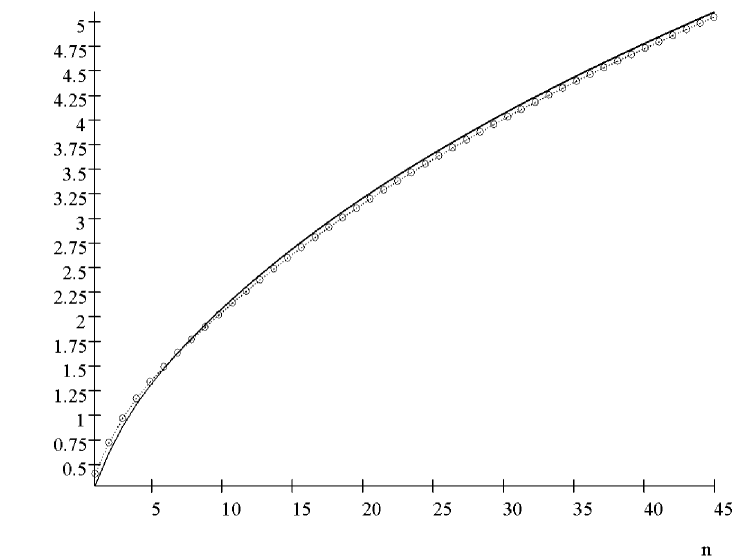
Figure 1: The expected average sensitivity of a typical monotone Boolean function versus the number of variables $n$. The cases of even $n$ (solid line) and odd $n$ (line with circles) are shown separately.

4 Stack filter performance in terms of dynamical behavior

To relate the noise suppression properties of a stack filter to the dynamical behavior, captured by the average sensitivity, we filtered various test signals and noise distributions with all five-input stack filters. Figures 2 and 3 show the mean square error (MSE) as a function of filter sensitivity for blocks and Heaviside signals, respectively. In addition, Figure 4 shows the MSE performance for different degrees of salt and pepper noise.

(a)	(b)

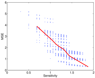
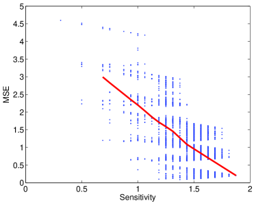
Figure 2: Mean square error versus sensitivity of stack filter. Data is shown for blocks signal under (a) Gaussian and (b) bimodal noise (see [13] for details on noise distributions).

(a)	(b)

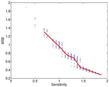
Figure 3: Mean square error versus sensitivity of stack filter. Data is shown for Heaviside signal under (a) Gaussian and (b) bimodal noise.

(a)	(b)	(c)

Figure 4: Mean square error versus sensitivity of stack filter. Data is shown for Heaviside signal under salt and pepper noise with probability (a) 0.001, (b) 0.01 and (c) 0.1.

Based on these results, it is clear that filters that are chaotic, in terms of their sensitivity, perform best under various noise conditions. Simulations with salt and pepper noise show that as more noise is added, the performance of ordered and critical filters deteriorate more that the chaotic ones.

In light of what we known about the dynamics of random Boolean networks, this observation is somewhat surprising. A large body of work with Boolean networks has established that dynamically critical systems are the ones that strike the optimal compromise between robustness to noise and reliable propagation of information. Thus, it would be expected that dynamically critical stack filters would have performed optimally under variable noise conditions in terms of noise suppression and detail preservation.

There are several aspects of signal denoising that are essentially distinct from the analysis of dynamical systems. The theory, which relates the average sensitivity of a Boolean network to the dynamical regimes, is based on the propagation of small perturbations. That is, to quantify the dynamical behavior, we measure whether small perturbations that are introduced into the state of the system are amplified or attenuated, leading to chaotic or ordered behavior, respectively.

Noise filtering is fundamentally different in terms of what we know about propagation of small perturbations. A noisy signal is frequently the result of a large perturbation that has affected the value of majority of the signal values (consider additive or multiplicative noise that affects every signal value or pixel). Thus, the insights derived from the small perturbation analysis of dynamical systems do not necessary hold. The mean squared error of the filter does not necessary capture the trade-off between noise suppression and detail preservation that is observed when small perturbations are studied. Very little is known about the dynamical systems behavior when only the observations about the response to large perturbations are available.

4.1 Stack filter as a generalization of a monotone Boolean network

An important aspect of stack filters is that they can be viewed as a generalization of the monotone Boolean network model to a continuos model. As a stack filter corresponds to a monotone Boolean function and filtering can be implemented in the form of a Boolean network, the stack filter forms a network that can be run for continuos signals. This insight gives an interesting possibility to analyze the relationships between Boolean and continuos models.

Recently, there have been several attempts to link the properties of Boolean networks to the behavior of classes of continuous or more detailed discrete models. For example, the existence of dynamical regimes has been demonstrated in models other than Boolean networks. The interpretation of stack filters as generalizations of Boolean networks allows us to study the connections between Boolean and continuos models directly.

In recent work [4], we introduced an information theory based order parameter that can, in principle, be used to quantify the dynamical behavior of any model class, discrete or continuous. This parameter measures the average tendency of the dynamical system to attenuate or amplify informational distances (computed using real world compressors) between states of the system. We utilize this order parameter to quantify the dynamical behavior of stack filters in both the binary and continuos forms. In the binary case, we introduce single bit perturbations to states of the system with varying probability. In this standard analysis, the information theory-based order parameter has been shown to accurately capture the dynamical behavior, characterized by the average sensitivity of the Boolean function [4]. For the continuous case, we can introduce noise in the form of salt and pepper noise with varying probability. Results for the continuous case are shown in Figure 5.

(a)	(b)	(c)

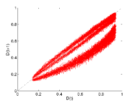
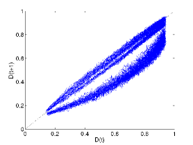
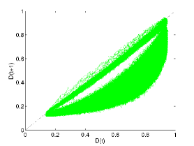
Figure 5: Information theoretical order parameter (Derrida curve) computed for continuous signals. (a), (b) and (c) show filter classes that are ordered, critical and chaotic in terms of the average sensitivity of the Boolean function implementing the stack filter, respectively. All $K=5$ stack filters are shown. $D(t)$ is the information distance between two input signals and $D(t+1)$ is the distance between filtered signals. Each line is the averaged behavior of a single stack filter. See [4] for the details on the construction of the Derrida curve.

Remarkably, this analysis suggests that the dynamical regimes of the networks are different when the input data are changed from binary to continuous. For example, a Boolean network that is chaotic in terms of average sensitivity (and confirmed with the information distance -based order parameter) may not be chaotic in the continuous domain in terms of the same information distance -based order parameter. This suggests that the properties that are derived for the monotone Boolean functions do not necessary hold when the function is generalized to the continuous case.

5 Conclusions

We have shown an analytical relationship between stack filter design coefficients $A_{i}$ and the average sensitivity of the monotone Boolean function. In addition, we presented a formula for the average sensitivity of typical monotone Boolean functions. This formula implies that typical stack filters are dynamically chaotic.

These results suggest a novel perspective that can potentially be utilized in the design of stack filters for specific filtering tasks. It ties the design of stack filters to a more general dynamical systems framework. Thus, we can also utilize stack filter optimization algorithms to design Boolean networks that are statistically optimal under given noise distributions. It will be of interest to compare the properties of such statistically optimal ensembles of networks to the properties of other ensembles under different noise conditions. By estimating the noise distributions from biological data and designing optimal Boolean networks may also help us gain insight into the dynamical behavior of biological systems.

We also studied the behavior of stack filters under various noise distributions by relating the MSE to the average sensitivity of the filter. This analysis suggests that chaotic filters perform best under various noise conditions. This is contradictory to what was expected based on our knowledge about Boolean networks. However, subsequent analysis shed light on this observation. Dynamics of Boolean networks are defined under the assumption of small perturbations while the filtering of noisy signals is a fundamentally different problem. In addition, our parallel analysis of stack filter dynamics in Boolean and continuous cases suggests that the dynamical behavior of monotone Boolean functions does not directly generalize to continuous systems.

Future work should focus on understanding these aspects in more detail. More work needs to be done to be able to quantify the dynamics of a system from large perturbations. It will also be of interest to study the connections between dynamical behavior of Boolean and continuous models. Stack filters will be a useful model class for these studies due to the availability of direct generalizations from the Boolean to the continuous domain.

References

- [1] S. A. Kauffman, The Origins of Order: Self-organization and selection in evolution. New York: Oxford University Press, 1993.
- [2] R. Serra, M. Villani, and A. Semeria, “Genetic network models and statistical properties of gene expression data in knock-out experiments,” J. Theor. Biol., vol. 227, no. 1, pp. 149–157, Mar. 2004.
- [3] P. Rämö, J. Kesseli, and O. Yli-Harja, “Perturbation avalanches and criticality in gene regulatory networks,” J. Theor. Biol., vol. 242, no. 1, pp. 164–170, Mar. 2006.
- [4] M. Nykter, N. D. Price, M. Aldana, S. Ramsey, S. A. Kauffman, L. Hood, O. Yli-Harja, and I. Shmulevich, “Gene expression dynamics in the macrophage exhibit criticality,” Proc. Natl. Acad. Sci. USA, vol. 105, no. 6, pp. 1897–1900, Feb. 2008.
- [5] P. Krawitz and I. Shmulevich, “Basin entropy in boolean network ensembles,” Phys. Rev. Lett., vol. 98, no. 158701, 2007.
- [6] A. S. Ribeiro, S. A. Kauffman, J. Lloyd-Price, B. Samuelsson, and J. E. S. Socolar, “Mutual information in random Boolean models of regulatory networks,” Phys. Rev. E, vol. 77, no. 011901, 2008.
- [7] M. Nykter, N. D. Price, A. Larjo, T. Aho, S. A. Kauffman, O. Yli-Harja, and I. Shmulevich, “Critical networks exhibit maximal information diversity in structure-dynamics relationships,” Phys. Rev. Lett., vol. 100, no. 058702, Feb. 2008.
- [8] I. Shmulevich and E. R. Dougherty, “Genetic regulatory networks: A nonlinear signal processing perspective,” in Nonlinear Signal and Image Processing: Theory, Methods, and Applications, K. Barner and G. Arce, Eds. CRC Press, 2003, pp. 507–523.
- [9] J. Astola and P. Kuosmanen, Fundamentals of Nonlinear Digital Filtering. CRC Press, 1997.
- [10] M. Gabbouj, E. J. Coyle, and N. Gallagher, “An overview of median and stack filtering,” Circuits, Systems, and Signal Proces., vol. 11, no. 1, pp. 7–45, 1992.
- [11] M. Gabbouj and E. J. Coyle, “Minimum mean absolute error stack filtering with structural constraints,” IEEE T. Acoust., Speech, vol. 38, pp. 955–968, 1990.
- [12] ——, “On the lp which finds a mmae stack filter,” IEEE T. Signal Proces., vol. 39, no. 11, pp. 2419–2424, 1991.
- [13] I. Shmulevich, V. Melnik, and K. Egiazarian, “The use of sample selection probabilities for stack filter design,” IEEE Signal Proc. Let., vol. 7, no. 7, pp. 189–192, Jul. 2000.
- [14] A.-L. Barabási and R. Albert, “Emergence of scaling in random networks,” Science, vol. 286, no. 5439, pp. 509–512, Oct. 1999.
- [15] M. Aldana and P. Cluzel, “A natural class of robust networks,” Proc. Natl. Acad. Sci. USA, vol. 100, no. 15, pp. 8710–8714, Jul. 2003.
- [16] D. Stauffer, “On forcing functions in Kauffman random Boolean networks,” J. Stat. Phys., vol. 46, no. 3–4, pp. 789–794, 1987.
- [17] I. Shmulevich, H. Lähdesmäki, E. R. Dougherty, J. Astola, and W. Zhang, “The role of certain Post classes in Boolean network models of genetic networks,” Proc. Natl. Acad. Sci. USA, vol. 100, no. 19, pp. 10 734–10 739, 2003.
- [18] S. A. Kauffman, Investigations. New York: Oxford University Press, 2000.
- [19] S. E. Harris, B. K. Sawhill, A. Wuensche, and S. Kauffman, “A model of transcriptional regulatory networks based on biases in the observed regulation rules,” Complexity, vol. 7, no. 4, pp. 23–40, 2002.
- [20] A. Wuensche, “Discrete dynamical networks and their attractor basins,” Complexity International, vol. 6, pp. 2–23, Jan. 1999.
- [21] M. Aldana, S. Coppersmith, and L. P. Kadanoff, “Boolean dynamics with random couplings,” in Perspectives and Problems in Nonlinear Science, E. Kaplan, J. E. Marsden, and K. R. Sreenivasan, Eds. New York: Springer-Verlag, May 2003, pp. 23–89.
- [22] B. Derrida and Y. Pommeau, “Random networks of automata: A simple annealed approximation,” Europhys. Lett., vol. 1, pp. 45–49, 1986.
- [23] B. Luque and R. V. Sole, “Phase transitions in random networks: Simple analytic determination of critical points,” Phys. Rev. E, vol. 55, no. 1, pp. 257–260, Jan. 1997.
- [24] ——, “Lyapunov exponents in random Boolean networks,” Physica A, vol. 284, no. 1-4, pp. 33–45, 2000.
- [25] I. Shmulevich and S. A. Kauffman, “Activities and sensitivities in Boolean network models,” Phys. Rev. Lett., vol. 93, no. 4, p. 048701, 2004.
- [26] P. D. Wendt, E. J. Coyle, and N. C. Callagher, “Stack filters,” IEEE T. Acoust., Speech, vol. 34, pp. 898–911, 1986.
- [27] S. Agaian, J. Astola, and K. Egiazarian, Binary Polynomial Transforms and Non-linear Digital Filters. CRC Press, 1995.
- [28] P. Kuosmanen, “Statistical analysis and optimization of stack filters,” Ph.D. dissertation, Tampere University of Technology., Tampere, Finland, 1994.
- [29] I. Shmulevich, O. Yli-Harja, J. Astola, , and A. Korshunov, “On the robustness of the class of stack filters,” IEEE T. Signal Proces., vol. 50, no. 7, pp. 1640–1649, 2002.
- [30] K. Egiazarian, P. Kuosmanen, and J. Astola, “Boolean derivatives, weighted chow parameters, and selection probabilities of stack filters,” IEEE T. Signal Proces., vol. 44, no. 7, pp. 1634–1641, Jul. 1996.
- [31] I. Shmulevich, “Average sensitivity of typical monotone boolean functions,” arXiv math, vol. 0507030, 2005.