Anomalies, Beta Functions and Supersymmetric Unification with Multi-Dimensional Higgs Representations

Abstract

In the framework of supersymmetric Grand Unified Theories, the minimal Higgs sector is often extended by introducing multi-dimensional Higgs representations in order to obtain realistic models. However these constructions should remain anomaly-free, which constraints significantly their structure. We review the necessary conditions for the cancellation of anomalies in general and discuss in detail the different possibilities for SUSY SU(5) models. Alternative anomaly free combinations of Higgs representations, beyond the usual vector-like choice, are identified, and it is shown that their corresponding $\beta$ functions are not equivalent. Although the unification of gauge couplings is not affected, the introduction of multi-dimensional representations leads to different scenarios for the perturbative validity of the theory up to the Planck scale.

I Introduction

Supersymmetric Grand Unified Theories (SGUT) GeorgiGlashow74 ; Raby ; Mohapatra ; Raby2 have achieved some degree of success: unification of gauge couplings, charge quantization, prediction of the weak mixing angle, the mass-scale of neutrinos. Detection of weak scale superpartners or proton decay, as well as some patterns of FCNC/LFV and CP violation phenomena would indicate that some form of SGUT lays beyond the SM JLDC . Although this degree of success is already present in the minimal models (SO(10) or some variant of SU(5)) Murayama ; HMY93 ; Barr , there are open problems that suggest the need to incorporate more elaborate constructions HMTY , specifically the use of higher-dimensional representations in the Higgs sector (i.e. SU(5) representations with dimension $>24$). For instance, a 45 representation is often included to obtain correct mass relations for the first and second families of d-type quarks and leptons GeorgiJarlskog , while a 75 representation has been employed to address the doublet-triplet problem MuOkYa .

When one adds these higher-dimensional Higgs representation within the context of ${\cal N}=1$ SUSY GUTs, one must verify the cancellation of anomalies associated to their fermionic partners, i.e. the Higgsinos. The most straightforward solution to anomaly-cancellation is obtained by including vector-like representations i.e. including both $\psi$ and $\bar{\psi}$ chiral supermultiplets; up to our knowledge this seems to be the option chosen by most models builders. It is one of the purposes of this paper to find alternatives to this option, namely to create an anomaly free Higgs sector, including some representation $\psi$ and a set of other representations of lower-dimension $\left\{\phi_{1},\phi_{2},...\right\}$. It turns out that different anomaly-free combinations of representations are not equivalent in terms of their $\beta$ functions.

It is also known that the unification condition imposes some restrictions on the GUT-scale masses of the gauge bosons, gauginos, Higgses, and Higgsinos Terning2 . However the addition of complete GUT multiplets does not change the unified gauge couplings, and neither modifies the unification scale. On the other hand, the evolution of the gauge couplings above the GUT scale, up to the Planck scale, depends on the matter and Higgs content, thus the perturbative validity of the model is affected by the inclusion of additional multiplets. This is important in order to determine whether gravitational effects should be invoked for the viability of the model Calmet . In this paper we also study the effect of the higher-dimensional Higgs multiplets on the evolution of the gauge coupling up to the Planck scale, focusing on models that invoke different sets of representations in order to satisfy the anomaly-free conditions.

Our paper is organized as follows. In section II we review the different mechanisms proposed in the literature to get anomaly free gauge theories for general gauge groups. Focusing on SU(N)-type models, we look for new alternatives to anomaly cancellation. The implications of our results for specific SUSY GUT SU(5) models are presented in section III. The issue of gauge coupling unification, and the effect of higher-dimensional representations is discussed in section IV, where we include the 2-loop effect on the gauge unification that is brought by the Yukawa couplings associated with those representations at the 1-loop level. Finally our conclusions are presented in section V.

II Anomalies in gauge theories

Whether a symmetry that holds at the classical level is respected or not at the quantum level is signaled by the presence of anomalies. The importance of anomalies was recognized almost immediately after the proof that Yang-Mills theories with SSB are renormalizable was presented in Hooft Veltman . Anomalies can be associated with both global or local symmetries, the latter being most dangerous for the consistency of the theory. The so-called perturbative anomalies arise in abelian gauge symmetries while non-abelian symmetries can have anomalies of a non-perturbative origin that turn out to be of topological nature AdlerBellJackiw . The need to require anomaly cancellation in any gauge theory stems from the fact that their presence destroys the quantum consistency of the theory Bardeen . It turns out that all one needs in order to identify the anomaly is to calculate the triangle diagrams of the form AVV, with A=Axial, and V=Vector currents.

For a given fermionic representation $D$ of a gauge group $G$, the anomaly can then be written as Terning2 :

$$A(D)d^{abc}\equiv Tr\left[\left\{T_{a}^{D_{i}},T_{b}^{D_{i}}\right\}T_{c}^{D_{i}}\right],$$ (1)

where $T_{a}^{D_{i}}$ denotes the generators of the gauge group $G$ in the representation $D_{i}$, and $d^{abc}$ denotes the anomaly associated with the fundamental representation. The anomaly coefficients $a_{D}\equiv A(D)$ for the most common representations are shown in Table 1 for SU(N) groups; a result that is known in the literature Terning2 . In order to obtain these results one makes use of the following relations:

1. For a representation $R$ that is a direct sum of two representations, $R=R^{1}\oplus R^{2}$, the anomaly is given by

   $$A_{R}=A(R_{1}\oplus R_{2})=A(R_{1})+A(R_{2}).$$ (2)

2. For a representation $R$ that is the tensor product of two representations, the anomaly is given by:

   $$A_{R}=A(R)=A(R_{1}\otimes R_{2})=D(R_{1})A(R_{2})+D(R_{2})A(R_{1}),$$ (3)

   with $D(R_{i})$ denoting the dimensions of representations $R_{i}$.

Then, starting from the fundamental representations $F$, we have taken the tensor products and evaluated the unknown coefficients that appear in the products in terms of $A(F)$. The dimension of the representations has been verified using the chain notation $(\alpha,\beta,\gamma,\ldots)$. Results for some SU(N) representations can be read off from tables in Slansky . We have extended these results to include additional higher-dimensional representations, with the corresponding expressions shown in Table 2.

$$\begin{array}[]{|c|c|c|c|}\hline\cr Irrep&dim(r)&2T(r)&A(r)\\ \hline\cr\includegraphics[scale={.15}]{1.eps}&N&1&1\\ Ad&N^{2}-1&2N&0\\ \includegraphics[scale={.15}]{2.eps}&\frac{N(N-1)}{2}&N-2&N-4\\ \includegraphics[scale={.15}]{11.eps}&\frac{N(N+1)}{2}&N+2&N+4\\ \includegraphics[scale={.15}]{3.eps}&\frac{N(N-1)(N-2)}{6}&\frac{(N-3)(N-2)}{2}&\frac{(N-3)(N-6)}{2}\\ \includegraphics[scale={.15}]{111.eps}&\frac{N(N+1)(N+2)}{6}&\frac{(N+2)(N+3)}{2}&\frac{(N+3)(N+6)}{2}\\ \includegraphics[scale={.15}]{21.eps}&\frac{N(N-1)(N+1)}{3}&N^{2}-3&N^{2}-9\\ \includegraphics[scale={.15}]{22.eps}&\frac{N^{2}(N+1)(N-1)}{12}&\frac{N(N-2)(N+2)}{3}&\frac{N(N-4)(N+4)}{3}\\ \includegraphics[scale={.15}]{1111.eps}&\frac{N(N+1)(N+2)(N+3)}{24}&\frac{(N+2)(N+3)(N+4)}{6}&\frac{(N+3)(N+4)(N+8)}{6}\\ \includegraphics[scale={.15}]{31.eps}&\frac{N(N+1)(N-1)(N-2)}{8}&\frac{(N-2)(N^{2}-N-4)}{2}&\frac{(N-4)(N^{2}-N-8)}{2}\\ \hline\cr\end{array}$$

Table 1: Dimensions, Dynkin indexes, and anomaly coefficients for some representations of SU(N).

$$\begin{array}[]{|c|c|c|c|}\hline\cr Irrep&dim(r)&A(r)\\ \hline\cr\includegraphics[scale={.15}]{4.eps}&\frac{N(N-1)(N-2)(N-3)}{24}&\frac{(N-4)(N-3)(N-8)}{6}\\ \includegraphics[scale={.15}]{11111.eps}&\frac{N(N+1)(N+2)(N+3)(N+4)}{120}&\frac{(N+3)(N+4)(N+5)(N+10)}{24}\\ \includegraphics[scale={.15}]{2111.eps}&\frac{N(N+1)(N+2)(N+3)(N-1)}{30}&\frac{(N-2)(N+3)(N+5)^{2}}{6}\\ \includegraphics[scale={.15}]{221.eps}&\frac{N^{2}(N+1)(N+2)(N-1)}{24}&\frac{N(N+5)(5N^{2}-3N-50)}{24}\\ \includegraphics[scale={.15}]{32.eps}&\frac{N^{2}(N+1)(N-1)(N-2)}{24}&\frac{N(N-5)(5N^{2}+3N-50)}{24}\\ \includegraphics[scale={.15}]{311.eps}&\frac{N(N+1)(N+2)(N-1)(N-2)}{20}&\frac{(N^{4}-17N^{2}+100)}{4}\\ \includegraphics[scale={.15}]{41.eps}&\frac{(N-3)(N-2)(N-1)N(N+1)}{30}&\frac{(N-5)^{2}(N-3)(N+2)}{6}\\ \includegraphics[scale={.15}]{5.eps}&\frac{N(N-1)(N-2)(N-3)(N-4)}{120}&\frac{(N-5)(N-4)(N-3)(N-10)}{24}\\ \includegraphics[scale={.15}]{111111.eps}&\frac{N(N+1)(N+2)(N+3)(N+4)(N+5)}{720}&\frac{(N+3)(N+4)(N+5)(N+6)(N+12)}{120}\\ \includegraphics[scale={.15}]{21111.eps}&\frac{N(N+1)(N+2)(N+3)(N+4)(N-1)}{144}&\frac{(N+3)(N+4)(N+6)(N^{2}+5N-12)}{24}\\ \includegraphics[scale={.15}]{2211.eps}&\frac{(N-1)N^{2}(N+1)(N+2)(N+3)}{80}&\frac{3}{40}(N-3)N(N+3)(N+4)(N+6)\\ \includegraphics[scale={.15}]{3111.eps}&\frac{(N-2)(N-1)N(N+1)(N+2)(N+3)}{72}&\frac{(N+3)(N^{4}+3N^{3}-16N^{2}-36N+144)}{12}\\ \includegraphics[scale={.15}]{2222.eps}&\frac{(N-1)N^{2}(N+1)^{2}(N+2)}{144}&\frac{(N-4)N(N+1)(N+3)(N+6)}{24}\\ \includegraphics[scale={.15}]{321.eps}&\frac{(N-2)(N-1)N^{2}(N+1)(N+2)}{45}&\frac{2}{15}(N-4)(N-3)N(N+3)(N+4)\\ \includegraphics[scale={.15}]{411.eps}&\frac{(N-3)(N-2)(N-1)N(N+1)(N+2)}{72}&\frac{(N-3)(N^{4}-3N^{3}-16N^{2}+36N+144)}{12}\\ \includegraphics[scale={.15}]{33.eps}&\frac{(N-2)(N-1)^{2}N^{2}(N+1)}{144}&\frac{(N-6)(N-3)(N-1)N(N+4)}{24}\\ \includegraphics[scale={.15}]{42.eps}&\frac{(N-3)(N-2)(N-1)N^{2}(N+1)}{80}&\frac{3}{40}(N-6)(N-4)(N-3)N(N+3)\\ \includegraphics[scale={.15}]{51.eps}&\frac{(N-4)(N-3)(N-2)(N-1)N(N+1)}{144}&\frac{(N-6)(N-4)(N-3)(N^{2}-5N-12)}{24}\\ \includegraphics[scale={.15}]{6.eps}&\frac{(N-5)(N-4)(N-3)(N-2)(N-1)N}{720}&\frac{(N-6)(N-5)(N-4)(N-3)(N-12)}{120}\\ \hline\cr\end{array}$$

Table 2: Dimensions and anomaly coefficients for higher-dimensional representations of SU(N).

Then, given the previous results, one can try to identify possible ways that will enable us to construct anomaly free models. As it has been considered in the literature GeorgiGlashow72 ; BanksGeorgi , there are several ways to obtain anomaly free theories, namely:

i)

The gauge group itself is safe, i.e. it is always free of anomalies. This happens, for instance, for SO(10) but not for SU(5).

ii)

The gauge group is a subgroup of an anomaly free group, and the representations form a complete representation of the anomaly free group. For instance, this happens in the SU(5) case for the $\mathbf{5}+\mathbf{\overline{10}}$ representations, which together are anomaly free, and this can be understood because they belong to the $\mathbf{16}$ representation of SO(10), i.e. under SU(5) the 16 decomposes as: $\mathbf{16=5+\overline{10}+1}$.

iii)

The fermionic representations appear in conjugate pairs, i.e., they are vector-like. This is the most common choice when the Higgs sector of SUSY GUT is extended . For instance, a $\mathbf{45}+\mathbf{\overline{45}}$ pair is considered to solve the problem associated with the wrong Yukawa unification for first and second families within SU(5) models.

Here, we shall show that there are also other accidental possibilities that result when several lower-dimensional Higgs multiplets contribute to the anomaly associated with a larger-dimensional Higgs representation. This will be illustrated with the SU(5) case in the following section.

III Anomaly Cancellation in SUSY SU(5)

Let us consider an SU(5) SUSY GUT model. There are three copies of $\mathbf{\overline{5}}$ and 10 representations to accommodate the three families of quarks and leptons. Breaking of the GUT group to the SM: $SU(5)\rightarrow SU(3)_{C}\times SU(2)_{L}\times U(1)$, is achieved by including a (chiral) Higgs supermultiplet in the adjoint representation (24). Regarding anomalies, the $\mathbf{\overline{5}}$ and 10 contributions cancel each other. This situation corresponds to case ii in the previous section, that results from the fact that the SU(5) gauge symmetry is a subgroup of SO(10). On the other hand, the 24 representation is itself anomaly free. The minimal Higgs sector needed to break the SM gauge group can be formed with a pair of 5 and $\mathbf{\overline{5}}$ representations, which is indeed vectorial and therefore anomaly free (this corresponds to case iii discussed above).

Now, within this minimal model with a Higgs sector consisting of 5+$\mathbf{\overline{5}}$, one obtains the mass relations $m_{d_{i}}=m_{e_{i}}$, which works well for the third family, but not for the second family, while it may or may not work for the first family, depending on whether or not one includes weak scale threshold effectsDMP . One way to solve this problem is to add a 45 representation, which couples to the d-type quarks but not to the up-type, and one then obtains the Georgi-Jarlskog factor GeorgiJarlskog needed for the correct mass relations. Most models that obtain these relations with an extended Higgs sector, include the conjugate representation in order to cancel the anomalies, i.e. $\mathbf{45}+\mathbf{\overline{45}}$  Pavel Fileviez . This is however not the only possibility, and this is one of the main results of our paper.

$$\begin{array}[]{|c|c|c|c|c|}\hline\cr Irrep&Multiplet&dim(r)&A(r)&2T(r)\\ \hline\cr\left[5\right]&(0,0,0,0)&1&0&0\\ \left[1\right]&(1,0,0,0)&5&1&1\\ \left[2\right]&(0,1,0,0)&10&1&3\\ \left[1,1\right]&(2,0,0,0)&15&9&7\\ \left[4,1\right]&(1,0,0,1)&24&0&10\\ \left[1,1,1\right]&(3,0,0,0)&35&44&28\\ \left[2,1\right]&(1,1,0,0)&40&16&22\\ \left[3,1\right]&(1,0,1,0)&45&6&24\\ \left[2,2\right]&(0,2,0,0)&50&15&35\\ \hline\cr\end{array}$$

Table 3: Dimension, anomaly coefficients, and Dynkin indexes for different representations of SU(5).

The results for the anomaly coefficients for some representations of SU(5) (and their conjugates) are shown in table 3; we can see that the 45 anomaly coefficient is 6. Then taking into consideration that the 5 and the 10 have the anomaly coefficient $A=1$, we can write down the following anomaly-free combinations

$$A(\mathbf{45})+A(\mathbf{\overline{45}})=0 \ ,$$ (4)

$$A(\mathbf{45})+6A(\mathbf{\overline{5}})=0 \ ,$$ (5)

$$A(\mathbf{45})+6A(\mathbf{\overline{10}})=0 \ .$$ (6)

Alternatively we can write a general anomaly-free condition with these fields,

$$A(\mathbf{45})+fA(\mathbf{\overline{5}})+f^{\prime}A(\mathbf{\overline{10}})=0,\ \text{with }f+f^{\prime}=6\ .$$ (7)

One could also invoke a $\mathbf{\overline{15}}$ representation, which has $A=-9$, through the following anomaly-free combination:

$$A(\mathbf{45})+A(\mathbf{\overline{15}})+3A(\mathbf{5})=0\ .$$ (8)

These are non-equivalent models with different physical consequences. This is explicitly shown in the next section where we discuss the issue of gauge coupling unification.

IV Gauge coupling unification and perturbative validity.

The $\beta$ functions for a general SUSY theory with gauge group $G$ and matter fields appearing in chiral supermultiplets, at the 1-loop level, are given by:

$$\beta_{1}=\sum_{R}T_{R}-3C_{A},$$ (9)

where $T_{R}$ denotes the Dynkin index for the representation $R$, and $C_{A}$ is the quadratic Casimir invariant for the adjoint representation. For SU(N) type gauge groups $C_{A}=N$, while the $T_{R}$ index for most common SU(5) representations are also shown in Table 3.

The RGE’s with 1-loop $\beta$ functions for the gauge couplings of the MSSM are

$$\frac{d\alpha_{i}}{dt}=\beta_{i}\alpha_{i}^{2},$$ (10)

where

$$\beta_{i}=\left(\begin{array}[]{c}33/5\\ 1\\ -3\\ \end{array}\right)+\beta^{X}$$ (11)

and $t=(2\pi)^{-1}\ln M$, with $M=$ mass scale. The index $i=1,2,3$ refers to the U(1), SU(2) and SU(3) gauge groups respectively. The term $\beta^{X}=\sum_{\Phi}T(\Phi)$ denotes the contributions of the additional representations beyond those included in the MSSM (the sum is over all SU(5) additional multiplets $\Phi$). Assuming $M_{SUSY}\approx M_{t}$, one obtains that the unified gauge coupling is approximately $g(M_{GUT})=0.0416$, and unification occurs at $M_{GUT}=2\times 10^{16}$ GeV Hempfling .

These simple 1-loop results can be improved by using the 2-loop RGEs Jones:1981we ; Yamada:1993ga ; Barger:1992ac . In such case we solve numerically the corresponding RGE and we find that at the GUT scale $M_{GUT}=1.28\times 10^{16}$ GeV, the unified gauge coupling is $g_{5}(M_{GUT})=0.040$, and $h^{t}(M_{GUT})=0.6572$.

Now we are interested in evaluating the effect of the different representations in the running from $M_{GUT}$ up to the Planck scale. Besides evaluating the effect of the different anomaly free combinations, we are also interested in finding which representations are perturbatively valid up to the Planck scale. The unified gauge coupling obeys the 1-loop RGE

$$\mu\frac{d\alpha_{5}^{-1}}{d\mu}=\frac{-\beta_{1}}{2\pi}=\frac{3-\beta^{X}}{2\pi}\ ,$$ (12)

where $-\beta_{1}=\beta_{MIN}-\beta^{X}$, with $\beta_{MIN}=3$ denoting the contribution to the SU(5) $\beta$ function from the MSSM multiplets, including the one from the gauge sector.

The 1-loop $\beta$ functions for some interesting anomaly-free combinations are found to be:

$$\beta^{X}(\mathbf{45}+\mathbf{\overline{45}}) = 24\ ,$$

$$\beta^{X}(\mathbf{45}+6(\mathbf{\overline{5}})) = 15\ ,$$

$$\beta^{X}(\mathbf{45}+6(\mathbf{\overline{10}})) = 21\ ,$$

$$\beta^{X}(\mathbf{45}+\mathbf{\overline{15}}+2(\mathbf{10})+\mathbf{5}) = 19\ ,$$

$$\beta^{X}(\mathbf{50}+\mathbf{\overline{40}}+\mathbf{5}) = 29\ .$$ (13)

As shown in Figure 1, the model with $\beta^{X}=29$ induces a running of the unified gauge coupling that blows at the scale $M=6.61\times 10^{18}$ GeV, while for $\beta^{X}=24$ this happens at $M=2.63\times 10^{19}$ GeV. The models with $\beta^{X}=15,19,21$ are found to evolve safely all the way up to the Planck scale.

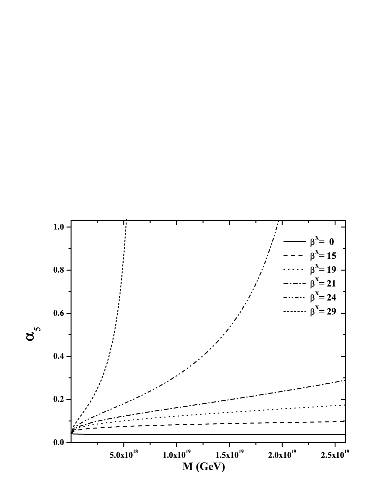
Figure 1: Evolution of the unified gauge coupling for the free anomaly combinations listed in the text. The evolution is shown all the way up to the Planck scale.

It is also interesting to consider the RGE effect associated with the Yukawa coupling that involve the additional Higgs representations. In order to do this we shall consider the 2-loop $\beta$ functions for the gauge coupling Martin:1993zk , but will keep only the 1-loop RGE for the new Yukawa couplings. Thus, we shall consider the following superpotential for the SUSY SU(5) GUT model:

$$W = \frac{f}{3}Tr\Sigma^{3}+\frac{1}{2}fVTr\Sigma^{2}+\lambda\bar{H}_{\alpha}(\Sigma^{\alpha}_{\beta}+3V\delta^{\alpha}_{\beta})H^{\beta}$$ (14)

$$+ \frac{h^{ij}}{4}\varepsilon_{\alpha\beta\gamma\delta\epsilon}\psi^{\alpha\beta}_{i}\psi^{\gamma\delta}_{j}H^{\epsilon}+\sqrt{2}f^{ij}\psi^{\alpha\beta}_{i}\phi_{j\alpha}\bar{H}_{\beta}\ .$$

Note that this superpotential involves the Higgs representations $\mathbf{5}$, $\bar{\mathbf{5}}$ y $\mathbf{24}$.

The 1-loop RGEs for the Yukawa parameters are given by HMY93 :

$$\mu\frac{d\lambda}{d\mu} = \frac{1}{(4\pi)^{2}}\left(-\frac{98}{5}g_{5}^{2}+\frac{53}{10}\lambda^{2}+\frac{21}{40}f^{2}+3(h^{t})^{2}\right)\lambda,$$ (15)

$$\mu\frac{df}{d\mu} = \frac{1}{(4\pi)^{2}}\left(-30g_{5}^{2}+\frac{3}{2}\lambda^{2}+\frac{63}{40}f^{2}\right)f,$$ (16)

$$\mu\frac{dh^{t}}{d\mu} = \frac{1}{(4\pi)^{2}}\left(-\frac{96}{5}g_{5}^{2}+\frac{12}{5}\lambda^{2}+6(h^{t})^{2}\right)h^{t}\ ,$$ (17)

while the 2-loop RGE for the unified gauge coupling is given by:

$$\mu\frac{dg_{5}}{d\mu}=\frac{1}{(4\pi)^{2}}(-3g_{5}^{3})+\frac{1}{(4\pi)^{4}}\frac{794}{5}g_{5}^{5}-\frac{1}{(4\pi)^{4}}\left\{\frac{49}{5}\lambda^{2}+\frac{21}{4}f^{2}+12(h^{t})^{2}\right\}g^{3}\ .$$ (18)

We use values of the coefficients $\lambda$, $h^{t}$ and $f$ that are safe at the Planck scale, and look for their effects on the unified gauge coupling. The resulting evolution is shown in one of the lines in Figure 2, where we show the 1-loop results, as well as the the 2-loop results with and without the Yukawas 1-loop contributions. The parameters used in the plots are $M_{GUT}=1.28\times 10^{16}$ GeV, $\alpha(M_{GUT})=0.040$, $h^{t}(M_{GUT})=0.6572$, $\lambda(M_{GUT})=0.6024$, and $f(M_{GUT})=1.7210$. We notice that there are appreciable differences for the evolution of the gauge coupling when going from the one to the 2-loop cases, but this difference is reduced when one includes Yukawa couplings at the 1-loop level.

Figure 2: Evolution of the unified gauge coupling for three different cases: i) the 1-loop result, ii) the 2-loop result without including Yukawas, and iii) the 2-loop result including the (1-loop) running of the Yukawas.

V Conclusions

We have studied the problem of anomalies in SUSY gauge theories in order to search for alternatives to the usual vector-like representations used in extended Higgs sectors. The known results have been extended to include higher-dimensional Higgs representations, which in turn have been applied to discuss anomaly cancellation within the context of realistic GUT models of SU(5) type. We have succeeded in identifying ways to replace the $\mathbf{45}+\bar{\mathbf{45}}$ models within SU(5) SUSY GUTs. Then, we have studied the $\beta$ functions for all the alternatives, and we find that they are not equivalent in terms of their values. We have also considered the RGE effect associated with the Yukawa coupling that involve the additional Higgs representations. We found that there are appreciable differences for the evolution of the gauge coupling when going from the 1 to the 2-loop RGE, but this difference is reduced when one includes the 1-loop Yukawa couplings at the 2-loop level. These results have important implications for the perturbative validity of the GUT models at scales higher than the unification scale.

- (1) H. Georgi and S. L. Glashow, Phys. Rev. Lett. 32, 438 (1974).
- (2) S. Raby, arXiv:hep-ph/0608183.
- (3) R. N. Mohapatra, arXiv:hep-ph/9911272.
- (4) S. Raby, Eur. Phys. J. C 59, 223 (2009) [arXiv:0807.4921 [hep-ph]].
- (5) J. L. Diaz-Cruz, Prepared for 5th Mexican Workshop of Particles and Fields, Puebla, Mexico, 30 Oct - 3 Nov 1995
- (6) H. Murayama and A. Pierce, Phys. Rev. D 65, 055009 (2002) [arXiv:hep-ph/0108104].
- (7) J. Hisano, H. Murayama and T. Yanagida, Nucl. Phys. B 402, 46 (1993) [arXiv:hep-ph/9207279].
- (8) C. H. Albright and S. M. Barr, Phys. Rev. D 62, 093008 (2000) [arXiv:hep-ph/0003251]; C. H. Albright and S. M. Barr, arXiv:hep-ph/0007145.
- (9) J. Hisano, T. Moroi, K. Tobe and T. Yanagida, Mod. Phys. Lett. A 10, 2267 (1995) [arXiv:hep-ph/9411298].
- (10) H. Georgi and C. Jarlskog, Phys. Lett. B 86, 297 (1979).
- (11) H. Murayama, Y. Okada and T. Yanagida, Prog. Theor. Phys. 88, 791 (1992).
- (12) J. Terning, Modern Supersymmetry, Dinamics and Duality, Oxford Science Publications,(2006); U. Sarkar, Int. J. Mod. Phys. A 22, 931 (2007) [arXiv:hep-ph/0606206].
- (13) X. Calmet, S. D. H. Hsu and D. Reeb, AIP Conf. Proc. 1078, 432 (2009) [arXiv:0809.3953 [hep-ph]].
- (14) G. ’t Hooft and M. J. G. Veltman, NATO Adv. Study Inst. Ser. B Phys. 4, 177 (1974).
- (15) S. L. Adler, Phys. Rev. 177, 2426 (1969); J. S. Bell and R. Jackiw, Nuovo Cim. A 60, 47 (1969).
- (16) William A. Bardeen, The Nonabelian Anomaly, J.J.Sakurai Prize Lecture Indianapolis APS Meeting, May 4, (1996); W. A. Bardeen, Lect. Notes Phys. 558, 3 (2000).
- (17) R. Slansky, Phys. Rept. 79, 1 (1981).
- (18) H. Georgi and S. L. Glashow, Phys. Rev. D 6, 429 (1972).
- (19) J. Banks and H. Georgi, Phys. Rev. D 14, 1159 (1976).
- (20) P. Fileviez Perez, arXiv:0710.1321 [hep-ph]; P. Fileviez Perez, Phys. Rev. D 76, 071701 (2007) [arXiv:0705.3589 [hep-ph]].
- (21) R. Hempfling, Phys. Lett. B 351, 206 (1995) [arXiv:hep-ph/9502201].
- (22) D. R. T. Jones, Phys. Rev. D 25, 581 (1982).
- (23) Y. Yamada, Phys. Rev. Lett. 72, 25 (1994) [arXiv:hep-ph/9308304].
- (24) V. D. Barger, M. S. Berger and P. Ohmann, Phys. Rev. D 47, 1093 (1993) [arXiv:hep-ph/9209232].
- (25) S. P. Martin and M. T. Vaughn, Phys. Rev. D 50, 2282 (1994) [Erratum-ibid. D 78, 039903 (2008)] [arXiv:hep-ph/9311340].
- (26) J. L. Diaz-Cruz, H. Murayama and A. Pierce, Phys. Rev. D 65, 075011 (2002) [arXiv:hep-ph/0012275].