Quantum theory of Synchronously Pumped type I Optical Parametric Oscillators: characterization of the squeezed supermodes

Abstract

Quantum models for synchronously pumped type I optical parametric oscillators (SPOPO) are presented. The study of the dynamics of SPOPOs, which typically involves millions of coupled signal longitudinal modes, is significantly simplified when one considers the “supermodes”, which are independent linear superpositions of all the signal modes diagonalizing the parametric interaction. In terms of these supermodes the SPOPO dynamics becomes that of about a hundred of independent, single mode degenerate OPOs, each of them being a squeezer. One derives a general expression for the squeezing spectrum measured in a balanced homodyne detection experiment, valid for any temporal shape of the local oscillator. Realistic cases are then studied using both analytical and numerical methods: the oscillation threshold is derived, and the spectral and temporal shapes of the squeezed supermodes are characterized.

I Introduction

Mode-locked trains of pulses, or frequency combs, have at the same time the coherence properties of c.w. lasers and the high peak powers of pulsed lasers. They are potentially perfect tools for generating non-classical states of light, as they are are at the same time high quality light sources, free of excess noise, and intense sources able to induce strong nonlinear effects, and therefore to generate strongly non-classical states of light, such as squeezed or quadrature-entangled states.

Frequency combs have been used in many quantum optics experiments, and have efficiently produced non classical light, either in $\chi^{(2)}$ Grangier ; ManipSPOPO6 ; Serkland or $\chi^{(3)}$ Watanabe ; Rosenbluh ; Friberg ; Schmitt ; Krylov ; Hirosawa ; Sharping ; Fiorentino media, but so far in a single-pass configuration in the nonlinear medium. In this configuration, one needs very high peak powers, and the system loses somehow its potential high quality in terms of pulse to pulse coherence and transverse profile. Mode locked lasers have also been used to efficiently generate squeezed states in optical fibers Levenson ; Shelby . The system has the drawback of generating non-minimal states states of light, because of the excess noise due to Brillouin scattering in the fiber.

We have recently proposed ourSPOPO06 to use synchronous optical cavities to recirculate the light in the nonlinear medium, thus enhancing further the nonlinear effects and imposing the cavity mode structure to the generated non-classical field. This can be done by building “synchronously pumped OPOs” or SPOPOs. In a SPOPO the cavity round-trip time is equal to the delay between successive pulses of the pumping mode-locked laser, so that the effect of the successive intense pump pulses add coherently, thus reducing considerably its oscillation threshold. In ourSPOPO06 , a large squeezing effect was predicted in some “supermodes”, which are well defined linear combinations of signal modes of different frequency, but not studied in detail. In the time domain these supermodes correspond to trains of pulses of different waveforms, orthogonal each other. The purpose of this paper is to precise the quantum model used to predict the effects and to investigate in a detailed way, through analytical or numerical methods, the potentialities of the system in realistic situations

SPOPOs have already been implemented as efficient sources of tunable ultra-short pulses manipSPOPO0 ; manipSPOPO1 ; manipSPOPO2 ; manipSPOPO3 ; manipSPOPO4 ; manipSPOPO5 their temporal properties have been theoretically investigated theorySPOPO1 ; theorySPOPO3 ; theorySPOPO4 , and actively mode-locking of OPOs has been recently achieved Fabien .

The decomposition of a pulsed field in terms of a basis of normal modes, similar to the supermodes we consider in this paper, has been introduced in different contexts for a complete quantum characterization of either the pulsed squeezed light generated by parametric down conversion BB ; Polish or solitons in optical fibers Opatrny2002 . Such approaches are strongly connected with the Schmidt decomposition of two-photon states for the characterization of pairwise entanglement Huang1996 ; Law2000 and the Bloch-Messiah reduction of any optical circuit characterized by a linear input-output relation Braunstein2005 . In this context Menicucci et al. Menicucci2008 proposed optical frequency combs as scalable resources for quantum computation.

The article is organized as follows: we present first the model that we will use. The system turns out to be characterized by a real and symmetric matrix $\mathcal{L}$, which contains all the information about the effective nonlinear interaction. The eigensystem of $\mathcal{L}$ is thus of special relevance and is studied in Section III, where the SPOPO threshold and several general properties of the spectrum of $\mathcal{L}$ are addressed. An analytical approximation to the diagonalization is also given that allows a better insight into the general trends as parameters are varied. In Section IV it is shown that the introduced eigenmodes or supermodes are squeezed, the corresponding eigenvalues determining the amount of squeezing, which can be measured in a balanced homodyne detection experiment that uses as the local oscillator (LO) a field with the same spectrum as the desired supermode. In Section V one then studies the squeezing properties of SPOPOs in two realistic cases, corresponding to BIBO and KNbO₃ crystals, using an appropriate scaling property of the diagonalization problem. Finally, an appendix details the case of the singly resonant SPOPO.

II The SPOPO model

II.1 Evolution equations for the operators

We consider quasi-degenerate collinear type I interaction, by means of which the pumping frequency comb, at frequencies around $2\omega_{0}$, is converted by a nonlinear $\chi^{\left(2\right)}$ crystal into multimode signal radiation at frequencies around $\omega_{0}$, and vice-versa, where $2\omega_{0}$ and $\omega_{0}$ are the two frequencies at which perfect phase matching occurs. This implies that one has $n\left(2\omega_{0}\right)=n\left(\omega_{0}\right)\equiv n_{0}$, where $n$ is the crystal refractive index. The nonlinear crystal is placed inside a high finesse optical cavity of length $L$, which is assumed to be dispersion compensated by intracavity dispersive elements, so that all cavity modes around the frequency $\omega_{0}$ are equally spaced by a common free spectral range $\Omega$, which is made equal to that of the pumping laser, thus warranting the synchronization of the pump to the OPO cavity. This ensures that the pulse-to-pulse delay of the pump beam coincides with the cavity round-trip time and successive pump and signal pulses superpose in time, thus maximizing the strength of the interaction. Hence the external pump mean field, which is a phase-locked multimode coherent field, can be written as

$$E_{\mathrm{ext}}\left(t\right)=\sqrt{\frac{P}{2\varepsilon_{0}c}}\sum_{m}i\alpha_{m}e^{-i\left(2\omega_{0}+m\Omega\right)t}+\mathrm{c.c.},$$ (1)

$P$ is the average laser irradiance (power per unit area), $\alpha_{m}$ is the normalized ($\sum\nolimits_{m}\left|\alpha_{m}\right|^{2}=1$) complex spectral component of longitudinal mode labeled by the integer index $m$, and $m=0$ corresponds to the phase-matched mode. As we will be concerned with femtosecond lasers with pulse durations around $100$fs , the number of pump modes will be typically on the order of $10^{4}-10^{5}$.

Two possibilities for pumping can be used: either (i) the pump also resonates inside the cavity (doubly resonant case), which requires in addition dispersion compensation at the pump spectral region, or (ii) the cavity is transparent for the pump (singly resonant case), a case which is free from the previous restriction and thus more amenable for experimentation, at the expense of a higher threshold, as we will see. We detail more the latter case in the appendix at the end of this paper. We will limit here our analysis to non-chirped pumps as chirping requires a more general treatment which will be presented elsewhere.

As the finesse of the cavity is assumed to be high, the intracavity signal field operator $\hat{E}_{\mathrm{s}}$ can be written as a superposition of cavity modes. Inside the $\chi^{\left(2\right)}$ crystal, which extends from $z=-l/2$ to $z=+l/2$, one can write

$$\hat{E}_{\mathrm{s}}(z,t)=\sum\limits_{m}i\mathcal{E}_{\mathrm{s},m}\hat{s}_{m}(t)u_{m}\left(z\right)e^{-i\omega_{\mathrm{s},m}t}+\mathrm{H.c.}$$ (2)

where $\omega_{\mathrm{s},m}=\omega_{0}+m\Omega$, $\hat{s}_{m}\left(t\right)$ is the annihilation operator for the $m$-th signal mode in the interaction picture, verifying standard boson commutation relations

$$\left[\hat{s}_{m}\left(t\right),\hat{s}_{n}^{{\dagger}}\left(t\right)\right]=\delta_{m,n},$$ (3)

$u_{m}\left(z\right)$ is the spatial profile of mode $m$, equal to $e^{ik_{\mathrm{s},m}z}$ in the case of ring cavities, while for linear cavities it is equal to $\sin\left[k_{\mathrm{s},m}\left(z+L/2\right)\right]$, where

$$k_{\mathrm{s},m}=k\left(\omega_{\mathrm{s},m}\right)=\frac{n\left(\omega_{\mathrm{s},m}\right)\omega_{\mathrm{s},m}}{c},$$ (4)

is the corresponding wavenumber. Finally $\mathcal{E}_{\mathrm{s},m}$ is the single photon field amplitude, whose value depends on the type of cavity. For a ring cavity

$$\mathcal{E}_{\mathrm{s},m}^{\left(\mathrm{ring}\right)}=\sqrt{\frac{\hbar\omega_{\mathrm{s},m}}{2\varepsilon_{0}n\left(\omega_{\mathrm{s},m}\right)A_{\mathrm{s}}L}},$$ (5)

where $A_{\mathrm{s}}$ is the transverse area of the signal field, while for a linear cavity

$$\mathcal{E}_{\mathrm{s},m}^{\left(\mathrm{linear}\right)}=\sqrt{2}\mathcal{E}_{\mathrm{s},m}^{\left(\mathrm{ring}\right)}.$$ (6)

Note that we are writing the field as a superposition of plane waves, but the treatment is approximately valid for Gaussian beams provided that the crystal is placed at the beam waist and the Rayleigh length is much longer than the crystal length $l$. In this case $A_{\mathrm{s}}=\pi w_{\mathrm{s}}^{2}$ with $w_{\mathrm{s}}$ the beam radius. Similarly we have $A_{\mathrm{p}}=\pi w_{\mathrm{p}}^{2}$ for the pump transverse mode.

The interaction Hamiltonian $\hat{H}_{\mathrm{I}}$ describing the parametric interaction in the nonlinear crystal is given as usual by:

$$\hat{H}_{\mathrm{I}}=-A_{\mathrm{I}}{\textstyle\int\limits_{-l/2}^{+l/2}}\mathrm{d}z\left[\hat{E}_{\mathrm{p}}\left(z,t\right)\hat{P}_{\mathrm{p}}\left(z,t\right)+\hat{E}_{\mathrm{s}}\left(z,t\right)\hat{P}_{\mathrm{s}}\left(z,t\right)\right],$$ (7)

where $\hat{P}_{\mathrm{s}}\left(z,t\right)$ and $\hat{P}_{\mathrm{p}}\left(z,t\right)$ are the nonlinear electric polarization at signal and pump frequencies, and $A_{\mathrm{I}}$ accounts for the effective area of interaction corresponding to the three-mode overlapping integral across the transverse plane and, for Gaussian beams, it is given by $A_{\mathrm{I}}^{-1}=A_{\mathrm{p}}^{-1}+2A_{\mathrm{s}}^{-1}$. The calculation of the Hamiltonian depends on the type of configuration (singly- or doubly resonant). Here we consider the simpler case of a doubly resonant SPOPO and leave the details of the singly resonant case for the Appendix.

II.1.1 Doubly resonant SPOPO

In this case an expression for the intracavity pump field operator $\hat{E}_{\mathrm{p}}$ analogous to (2), now centered around $2\omega_{0}$, can be used and the following expression for $\hat{H}_{\mathrm{I}}$ in the rotating wave approximation is obtained:

$$\begin{split}\hat{H}_{\mathrm{I}}=2i\varepsilon_{0}\chi lA_{\mathrm{I}}\sum_{m,q}&\mathcal{E}_{\mathrm{s},m}\mathcal{E}_{\mathrm{s},q}\mathcal{E}_{\mathrm{p},m+q}f_{m,q}\times\\ &\times\hat{s}_{m}^{{\dagger}}\left(t\right)\hat{s}_{q}^{{\dagger}}\left(t\right)\hat{p}_{m+q}\left(t\right)+\mathrm{H.c.,}\end{split}$$ (8)

where $\chi$ is the relevant nonlinear susceptibility, $\hat{p}_{m}\left(t\right)$ and $\hat{p}_{m}^{{\dagger}}\left(t\right)$ are pump boson operators ($m=0$ denotes the phase matched mode) verifying $\left[\hat{p}_{m}\left(t\right),\hat{p}_{m}^{{\dagger}}\left(t\right)\right]=\delta_{m,n}$, and $\mathcal{E}_{\mathrm{p},m}$ is as $\mathcal{E}_{\mathrm{s},m}$ with the substitutions $\omega_{\mathrm{s},m}\rightarrow\omega_{\mathrm{p},m}=2\omega_{0}+m\Omega$ and $A_{\mathrm{s}}\rightarrow A_{\mathrm{p}}$. The phase-mismatching factor of the crystal, $f_{m,q}$, is given by:

$$f_{m,q}=\frac{\sin\phi_{m,q}}{\phi_{m,q}},$$ (9)

$\phi_{m,q}$ being the phase-mismatch angle:

$$\phi_{m,q}=\frac{1}{2}\left(k_{\mathrm{p},m+q}-k_{\mathrm{s},m}-k_{\mathrm{s},q}\right)l.$$ (10)

Making use of the standard input-output formalism of optical cavities the following set of Heisenberg equations for the signal annihilation operators $\hat{s}_{m}$ is derived straightforwardly:

$$\frac{d\hat{s}_{m}}{dt}=-\gamma_{\mathrm{s}}\hat{s}_{m}+\sqrt{2\gamma_{\mathrm{s}}}\hat{s}_{\mathrm{in},m}+\kappa\sum\nolimits_{q}f_{m,q}\hat{s}_{q}^{{\dagger}}\hat{p}_{m+q},$$ (11)

where the cavity damping rate $\gamma_{\mathrm{s}}$, or cavity linewidth, is equal to $\frac{\Omega T_{\mathrm{s}}}{4\pi}$, $T_{\mathrm{s}}\ll 1$ is the transmission factor of the single cavity mirror at which losses are assumed to be concentrated, the coupling constant $\kappa$ is given by

$$\kappa=\mathcal{G}\chi l\frac{A_{\mathrm{I}}}{A_{\mathrm{s}}\sqrt{A_{\mathrm{p}}}}\left(\frac{\omega_{0}}{n_{0}L}\right)^{3/2}\sqrt{\frac{\hbar}{\varepsilon_{0}}},$$ (12)

and $\mathcal{G}$ is a factor depending on the geometry of the cavity that amounts to $2$ for the ring cavity and to $\sqrt{2}$ for the linear cavity.

Analogously, the evolution equations for the pump annihilation operators $\hat{p}_{q}$ are:

$$\frac{d\hat{p}_{q}}{dt}=-\gamma_{\mathrm{p}}\hat{p}_{q}+\sqrt{2\gamma_{\mathrm{p}}}\hat{p}_{\mathrm{in},q}-\frac{\kappa}{2}\sum\nolimits_{m}f_{m,q}\hat{s}_{m}\hat{s}_{q-m},$$ (13)

where $\gamma_{\mathrm{p}}$ is the cavity damping coefficient evaluated at pump frequencies.

To get these simple equations, we have assumed that $\mathcal{E}_{\mathrm{s},m}=\mathcal{E}_{\mathrm{s},0}$ $\forall m$, and neglected the dispersion of the nonlinear susceptibility, which is a very good approximation as far as the pulses bandwidth is not too large Seres . The “in” operators correspond to quantum fields entering the cavity through the coupling mirror. We consider the case where the input signal field is the vacuum, and the input pump field a coherent state. We have therefore $\left\langle\hat{s}_{\mathrm{in},m}\left(t\right)\right\rangle=0$, $\left\langle\hat{p}_{\mathrm{in},q}\left(t\right)\right\rangle=p_{\mathrm{ext},q}$, and the following correlations

$$\left\langle\hat{p}_{\mathrm{in},m}\left(t\right),\hat{p}_{\mathrm{in},m^{\prime}}^{{\dagger}}\left(t^{\prime}\right)\right\rangle = \left\langle\hat{s}_{\mathrm{in},m}\left(t\right),\hat{s}_{\mathrm{in},m^{\prime}}^{{\dagger}}\left(t^{\prime}\right)\right\rangle$$ (14)

$$= \delta_{m,m^{\prime}}\delta\left(t-t^{\prime}\right),$$

with the notation $\left\langle\hat{a},\hat{b}\right\rangle=\left\langle\left(\hat{a}-\left\langle\hat{a}\right\rangle\right)\left(\hat{b}-\left\langle\hat{b}\right\rangle\right)\right\rangle$, the rest of correlations being null. The mean input field $p_{\mathrm{ext},q}$ is related to the $\alpha_{q}$ and $P$ coefficients introduced in (1) by:

$$p_{\mathrm{ext},q}=\sqrt{\frac{n_{0}A_{\mathrm{p}}P}{2\hbar\omega_{0}}}\alpha_{q}.$$ (15)

II.1.2 Singly resonant SPOPO

As detailed in the Appendix, in the case where only the signal field is resonating into the cavity the evolution of the signal field annihilation operators is given by an expression identical to (11), but now the pump annihilation operators are given by

$$\begin{split}\hat{p}_{m}(t)=&\mathcal{G}\sqrt{\frac{L}{c}}\left(\hat{p}_{\mathrm{in},m}^{(+)}(t)+\hat{p}_{\mathrm{in},m}^{(-)}(t)\right)+\\ &-\mathcal{G}^{2}\frac{L}{c}\kappa\sum_{n}f_{n,m-n}\hat{s}_{n}(t)\hat{s}_{m-n}(t).\end{split}$$ (16)

We see that these operators contain two contributions. The first one corresponds to the free-field part that is described by means of two independent boson operators $\hat{p}_{\mathrm{in},m}^{(\pm)}(t)$ associated to the fields impinging the cavity from both the directions labeled with the superscripts $(\pm)$. We consider the unidirectional pumping case where the input pump field propagating from left to right (labeled with $(+)$) is a coherent state with a mean value of $\langle\hat{p}_{\mathrm{in},q}^{(+)}(t)\rangle=p_{\mathrm{ext},q}$, while the input pump field propagating form right to left (and labeled with $(-)$) is the vacuum $\langle\hat{p}_{\mathrm{in},q}^{(-)}(t)\rangle=0$. The mean input field, $p_{\mathrm{ext},q}$, is still given by Eq. (15), and the only non-null correlations are:

$$\left\langle\hat{p}_{\mathrm{in},m}^{(\pm)}\left(t\right),\left[\hat{p}_{\mathrm{in},n}^{(\pm)}\left(t^{\prime}\right)\right]^{{\dagger}}\right\rangle=\delta_{m,n}\,\delta\left(t-t^{\prime}\right).$$ (17)

II.2 The SPOPO below threshold

Below threshold signal modes have a zero mean value, whereas the pump field is characterized by a huge amplitude. One can therefore use a linearization procedure for the quantum fluctuations, which amounts to setting $\hat{p}_{m+q}\rightarrow\left\langle\hat{p}_{m+q}\right\rangle$ in (11). In the doubly resonant case $\left\langle\hat{p}_{m+q}\right\rangle=\sqrt{2/\gamma_{\mathrm{p}}}\left\langle\hat{p}_{\mathrm{in},m+q}\right\rangle=\sqrt{2/\gamma_{\mathrm{p}}}\,p_{\mathrm{ext},m+q}$, as given by (13), while in the singly resonant case $\left\langle\hat{p}_{m+q}\right\rangle=\mathcal{G}\sqrt{L/c}\left\langle\hat{p}_{\mathrm{in},m+q}^{\left(+\right)}\right\rangle=\mathcal{G}\sqrt{L/c}\,p_{\mathrm{ext},m+q}$, as given by (16). In both cases the final equations for the signal field anihilation operators are identical:

$$\frac{d\hat{s}_{m}}{dt}=-\gamma_{\mathrm{s}}\hat{s}_{m}+\sqrt{2\gamma_{\mathrm{s}}}\hat{s}_{\mathrm{in},m}+\gamma_{\mathrm{s}}\sigma\sum\nolimits_{q}\mathcal{L}_{m,q}\hat{s}_{q}^{{\dagger}},$$ (18)

where

$$\sigma=\sqrt{P/P_{0}},$$ (19)

is a pump amplitude parameter, and $P_{0}$ is an important scaling parameter for the pump, which can be shown to be the threshold value for the pump in the c.w. regime (single mode pump configuration). In the optimized configuration for the pump focussing ($A_{\mathrm{p}}=A_{\mathrm{s}}/2$), it is equal to:

$$P_{0}=\Pi_{0}\frac{\varepsilon_{0}c^{3}n_{0}^{2}T_{\mathrm{s}}^{2}}{2\left(\chi l\omega_{0}\right)^{2}},$$ (20)

$\Pi_{0}$	Doubly resonant	Singly resonant
Linear cavity	$T_{\mathrm{p}}/16$	$1$
Ring cavity	$T_{\mathrm{p}}/4$	$1$

Table 1: Coefficient for retrieving the cw threshold $P_{0}$ in the different experimental situations considered.

where $\Pi_{0}$ is given in Table 1 for the singly or doubly resonant configurations and ring or linear geometries. The differences arise from the fact that the doubly resonant case presents an intracavity pump power enhancement factor of $4/T_{\mathrm{p}}$ with respect to the singly resonant case and the crystal is used twice in a linear cavity as compared to the ring one. Hence the ratio $P_{0}^{\left(\mathrm{doubly}\right)}/P_{0}^{\left(\text{{singly}}\right)}$ equals the (very small) pump transmission factor of the doubly resonant cavity. By way of example, if we consider a singly resonant SPOPO (the geometry does not matter) based on a BIBO crystal BIBO with a thickness of $l=100\,\mu$m and pumped at $0.4\,\mu$m, we obtain reference irradiances $P_{0}$ of approximate values $14$, $344$, and $1400\,\mathrm{MW}\,\mathrm{cm}^{-2}$ for $T_{\mathrm{s}}=0.01$, $0.05$, and $0.1$, respectively. For a typical pump beam radius of $70\,\mu$m these irradiances lead to pump powers equal to $2$, $53$, and $212\,\mathrm{kW}$, respectively.

The key point for the following analysis is the fact that, in equations (18), the parametric coupling between the different signal modes is linear. It is characterized by a matrix $\mathcal{L}$, with matrix elements:

$$\mathcal{L}_{m,q}=f_{m,q}\alpha_{m+q}=\frac{\sin\phi_{m,q}}{\phi_{m,q}}\alpha_{m+q}.$$ (21)

When necessary, the phase mismatch angle $\phi_{m,q}$, Eq. (10) can be computed using a Taylor expansion around $2\omega_{0}$ for the pump wave vectors $k_{\mathrm{p},m}$ and around $\omega_{0}$ for the signal wave vectors $k_{\mathrm{s},m}$,

$$\phi_{m,q}\simeq\beta_{1}\left(m+q\right)+\beta_{2\mathrm{p}}\left(m+q\right)^{2}-\beta_{2\mathrm{s}}\left(m^{2}+q^{2}\right),$$ (22)

where

$$\beta_{1} =\frac{1}{2}\Omega\left(k_{\mathrm{p}}^{\prime}-k_{\mathrm{s}}^{\prime}\right)l,$$ (23)

$$\beta_{2\mathrm{p}} =\frac{1}{4}\Omega^{2}k_{\mathrm{p}}^{\prime\prime}l,$$ (24)

$$\beta_{2\mathrm{s}} =\frac{1}{4}\Omega^{2}k_{\mathrm{s}}^{\prime\prime}l,$$ (25)

are dispersion coefficients, and $k^{\prime}$ and $k^{\prime\prime}$ are the first and second derivatives of the wave vector with respect to frequency. Note that the matrix $\mathcal{L}$ depends on the cavity characteristics only through the free spectral range $\Omega$.

III SPOPO dynamics for the mean fields. Determination of the SPOPO threshold

Before calculating the quantum fluctuations of the SPOPO we analyze first the dynamics of the mean values of the operators, which is obtained by removing in Eq. (11) the input noise terms and replacing the operators by complex numbers:

$$\frac{ds_{m}}{dt}=-\gamma_{\mathrm{s}}s_{m}+\gamma_{\mathrm{s}}\sigma\sum\limits_{q}\mathcal{L}_{m,q}s_{q}^{\ast}.$$ (26)

The solution to Eqs. (26) is of the form

$$s_{m}\left(t\right)=S_{k,m}e^{\lambda_{k}t},$$ (27)

where $k$ is an index labelling the different solutions, and the parameters $S_{k,m}$ and $\lambda_{k}$ obey the following eigenvalue equation:

$$\lambda_{k}S_{k,m}=-\gamma_{\mathrm{s}}S_{k,m}+\gamma_{\mathrm{s}}\sigma\sum\limits_{q}\mathcal{L}_{m,q}S_{k,q}^{\ast}.$$ (28)

As matrix $\mathcal{L}$ is both self-adjoint and real, its eigenvalues $\Lambda_{k}$ and eigenvectors $\vec{L}_{k}$, of components $L_{k,m}$ defined by

$$\Lambda_{k}L_{k,m}=\sum\limits_{q}\mathcal{L}_{m,q}L_{k,q}$$ (29)

are all real. As $\gamma_{\mathrm{s}}$ and $\sigma$ are also real, it is evident that two sets of solutions to Eqs. (28) exist, namely $S_{k,m}^{\left(+\right)}=L_{k,m}$ and $S_{k,m}^{\left(-\right)}=iL_{k,m}$, with corresponding eigenvalues:

$$\lambda_{k}^{\left(\pm\right)}=\gamma_{\mathrm{s}}\left(-1\pm\sigma\Lambda_{k}\right).$$ (30)

Let us label by index $k=0$ the solution of maximum value of $|\Lambda_{k}|$. When $\sigma\left|\Lambda_{0}\right|<1$, all the rates $\lambda_{k}^{\pm}$ are negative, which implies that the null solution for the steady state signal field is stable. For simplicity of notation, we will take $\Lambda_{0}$ positive in the following, which is a common situation as shown below lam0 . Hence $\lambda_{0}^{\left(+\right)}$ is the largest eigenvalue and $\lambda_{0}^{\left(+\right)}=0$ sets the SPOPO oscillation threshold, which then occurs when the pump parameter $\sigma$ takes the value $1/\Lambda_{0}$, i.e. for a pump irradiance $P=P_{\mathrm{thr}}$ equal to:

$$P_{\mathrm{thr}}=P_{0}/\Lambda_{0}^{2}.$$ (31)

The exact value of $\Lambda_{0}$, and therefore of the SPOPO threshold, depends on the exact shape of the phase matching curve and on the exact spectrum of the pump laser. As will be shown in Sec. V, the theoretical SPOPO threshold can be extremely low, of the order of the cw single mode threshold divided by the number of pump modes.

Let us now define the normalized amplitude pumping rate $r$ by

$$r=\sqrt{P/P_{\mathrm{thr}}},$$ (32)

or $r=\sigma\Lambda_{0}$, so that the threshold occurs at $r=1$. The eigenvalues $\lambda_{k}$ become

$$\lambda_{k}^{\left(\pm\right)}=\gamma_{\mathrm{s}}\left(-1\pm r\frac{\Lambda_{k}}{\Lambda_{0}}\right).$$ (33)

We will call supermodes the set of $S_{k,m}$ values for a given $k$, which corresponds physically to the different spectral components of the signal field, and critical supermode $S_{k=0,m}^{\left(+\right)}$, the one associated with $\lambda_{0}^{\left(+\right)}$, which is the eigenvalue changing its sign at threshold. Above threshold, this critical mode will be the “lasing” one, i.e. the one having a non-zero mean amplitude when $r>1$. Note that the supermodes are independent of pump (Eq. 29),but not the eigenvalues (Eq. 30).

We note that the supermode in quadrature with respect to the critical one, $S_{0}^{\left(-\right)}=iS_{0}^{\left(+\right)}$, has an associated eigenvalue $\lambda_{0}^{\left(-\right)}=-2\gamma_{\mathrm{s}}$ at threshold, Eq. (33) with $r=1$, which is the lowest eigenvalue below- or at threshold. This property is obvious: Should $\lambda_{k}^{\left(-\right)}<-2\gamma_{\mathrm{s}}$ for some $k$, then $r\frac{\Lambda_{k}}{\Lambda_{0}}$ should be larger than $1$, what is incompatible with the fact that $\left|\frac{\Lambda_{k}}{\Lambda_{0}}\right|<1$ by definition and the condition $r<1$. The fact that there exists an eigenvector whose damping rate ($\lambda_{0}^{\left(-\right)}=-2\gamma_{\mathrm{s}}$ at threshold) is twice that of the passive cavity has important consequences on the squeezing properties of the SPOPO, as it occurs in other OPO configurations DOPOsoliton .

IV Quantum fluctuations of the SPOPO below threshold

IV.1 Fluctuation spectrum for the supermodes

We can now determine the quantum fluctuations of the signal field in a SPOPO below threshold. Let us introduce the following operators:

$$\hat{S}_{k}(t) =\sum\limits_{m}L_{k,m}\hat{s}_{m}(t),$$ (34)

$$\hat{S}_{\mathrm{in},k}(t) =\sum\limits_{m}L_{k,m}\hat{s}_{\mathrm{in},m}(t).$$ (35)

As $\vec{L}_{k}\cdot\vec{L}_{k^{\prime}}\equiv\sum\nolimits_{m}L_{k,m}L_{k^{\prime},m}=\delta_{k,k^{\prime}}$, one has trivially

$$\left[\hat{S}_{k}(t),\hat{S}_{k^{\prime}}^{\dagger}(t)\right] =\delta_{k,k^{\prime}},$$

$$\left[\hat{S}_{\mathrm{in},k}(t),\hat{S}_{\mathrm{in},k^{\prime}}^{\dagger}(t^{\prime})\right] =\delta_{k,k^{\prime}}\delta(t-t^{\prime}),$$

and the correlation

$$\left\langle\hat{S}_{\mathrm{in},k}(t),\hat{S}_{\mathrm{in},k^{\prime}}^{\dagger}(t^{\prime})\right\rangle=\delta_{k,k^{\prime}}\delta\left(t-t^{\prime}\right),$$ (36)

as well. Hence $\hat{S}_{k}$ and $\hat{S}_{\mathrm{in},k}$ are the annihilation operators of a combination of signal modes of different frequencies, which are the eigenmodes of the linearized evolution equation (26). The corresponding creation operator applied to the vacuum state creates a photon in a single supermode which globally describes the frequency comb, or train of pulses. Analogously one can define supermode output operators

$$\hat{S}_{\mathrm{out},k}(t)=\sum\limits_{m}L_{k,m}\hat{s}_{\mathrm{out},m}(t),$$ (37)

where the output boson operator $\hat{s}_{\mathrm{out},m}\left(t\right)$ relates to the intracavity and input boson operators through the usual input-output relation of high finesse optical cavities,

$$\hat{s}_{\mathrm{out},m}\left(t\right)=-\hat{s}_{\mathrm{in},m}\left(t\right)+\sqrt{2\gamma_{\mathrm{s}}}\hat{s}_{m}\left(t\right).$$ (38)

One can then write:

$$\frac{d}{dt}\hat{S}_{k}=-\gamma_{\mathrm{s}}\hat{S}_{k}+\gamma_{\mathrm{s}}\sigma\Lambda_{k}\hat{S}_{k}^{\dagger}+\sqrt{2\gamma_{\mathrm{s}}}\hat{S}_{\mathrm{in},k}.$$ (39)

Let us now define quadrature hermitian operators $\hat{S}_{k}^{\left(\pm\right)}$ by:

$$\hat{S}_{k}^{\left(+\right)} =\hat{S}_{k}+\hat{S}_{k}^{\dagger},$$ (40)

$$\hat{S}_{k}^{\left(-\right)} =-i\left(\hat{S}_{k}-\hat{S}_{k}^{\dagger}\right),$$ (41)

and analogously for $\hat{S}_{\mathrm{in},k}$ and $\hat{S}_{\mathrm{out},k}$, which obey the following equations:

$$\frac{d}{dt}\hat{S}_{k}^{\left(\pm\right)}=\lambda_{k}^{\left(\pm\right)}\hat{S}_{k}^{\left(\pm\right)}+\sqrt{2\gamma_{\mathrm{s}}}\hat{S}_{\mathrm{in},k}^{\left(\pm\right)},$$ (42)

with $\lambda_{k}^{\left(\pm\right)}$ given by Eq. (30). These relations enable us to determine the intracavity quadrature operators in the Fourier domain $\tilde{S}_{k}^{\left(\pm\right)}(\omega)$

$$i\omega\tilde{S}_{k}^{\left(\pm\right)}(\omega)=\lambda_{k}^{\left(\pm\right)}\tilde{S}^{\pm}(\omega)+\sqrt{2\gamma_{\mathrm{s}}}\tilde{S}_{\mathrm{in},k}^{\left(\pm\right)}(\omega).$$ (43)

Finally, the usual input-output relation on the coupling mirror (38), which can be written as

$$\tilde{s}_{\mathrm{out},m}(\omega)=-\tilde{s}_{\mathrm{in},m}(\omega)+\sqrt{2\gamma_{\mathrm{s}}}\tilde{s}_{m}(\omega),$$ (44)

being $\tilde{s}_{\mathrm{out},m}(\omega)$ the Fourier transform of the output boson operator $\hat{s}_{\mathrm{out},m}\left(t\right)$, extends by linearity to any supermode operator as the mirror is assumed to have a transmission independent of the mode frequency. One then obtains the following expression for the quadrature component in Fourier space of any signal supermode,

$$\tilde{S}_{\mathrm{out},k}^{\left(\pm\right)}(\omega) =v_{k}^{\left(\pm\right)}\left(\omega\right)\tilde{S}_{\mathrm{in},k}^{\left(\pm\right)}(\omega),$$ (45)

$$v_{k}^{\left(\pm\right)}\left(\omega\right) =\frac{\gamma_{\mathrm{s}}\left(1\pm r\Lambda_{k}/\Lambda_{0}\right)-i\omega}{\gamma_{\mathrm{s}}\left(-1\pm r\Lambda_{k}/\Lambda_{0}\right)+i\omega}.$$ (46)

One has also, for the operators in Fourier space:

$$\left\langle\tilde{S}_{\mathrm{in},k}^{\left(a\right)}\left(\omega_{1}\right)\tilde{S}_{\mathrm{in},l}^{\left(b\right)}\left(\omega_{2}\right)\right\rangle = \frac{\eta^{(a,b)}}{2\pi}\delta_{kl}\delta\left(\omega_{1}+\omega_{2}\right)$$ (47)

$$a = \pm,b=\pm$$ (48)

with $\eta^{(+,+)}=\eta^{(-,-)}=1$ and $\eta^{(+,-)}=-\eta^{(-,+)}=i$.

IV.2 Homodyne detection

The variances of the quadrature operators can be measured using the usual balanced homodyne detection scheme: the local oscillator (LO) is in the present case a coherent mode-locked multimode field $E_{\mathrm{L}}\left(t\right)$ having the same repetition rate as the pump laser:

$$E_{\mathrm{L}}\left(t\right) =E_{\mathrm{L}}^{-}\left(t\right)+E_{\mathrm{L}}^{+}\left(t\right)$$ (49)

$$E_{\mathrm{L}}^{-}\left(t\right) =i\epsilon_{\mathrm{L}}\sum_{m}e_{m}e^{-i\omega_{\mathrm{s},m}t},$$ (50)

$$E_{\mathrm{L}}^{+}\left(t\right) =\left[E_{\mathrm{L}}^{-}\left(t\right)\right]^{\ast},$$ (51)

where $\sum_{m}|e_{m}|^{2}=1$, and $\epsilon_{\mathrm{L}}$ is the LO field total amplitude factor. The output signal exiting the SPOPO, $\hat{E}_{s,\mathrm{out}}\left(t\right)$, is combined with $E_{\mathrm{L}}\left(t\right)$ in a 50%–50% beam splitter, the intensity of the two output ports is measured using photodiodes of unity quantum efficiency, and their difference constitutes the homodyne signal. Writing

$$\hat{E}_{s,\mathrm{out}}\left(t\right) =\hat{E}_{s,\mathrm{out}}^{-}\left(t\right)+\hat{E}_{s,\mathrm{out}}^{+}\left(t\right),$$

$$\hat{E}_{s,\mathrm{out}}^{-}\left(t\right) =i\mathcal{E}_{\mathrm{out}}\sum\nolimits_{n}\hat{s}_{\mathrm{out},m}\left(t\right)e^{-i\omega_{\mathrm{s},m}t},$$

$$\hat{E}_{s,\mathrm{out}}^{+}\left(t\right) =\left[\hat{E}_{s,\mathrm{out}}^{-}\left(t\right)\right]^{{\dagger}},$$

where $\mathcal{E}_{\mathrm{out}}$ is a proportionality constant. If sufficiently fast detectors were used the measurement would give an instantaneous signal represented by the operator

$$\hat{\imath}\left(t\right)=\frac{1}{\epsilon_{\mathrm{L}}\mathcal{E}_{\mathrm{out}}}\left[E_{\mathrm{L}}^{-}\left(t\right)\hat{E}_{s,\mathrm{out}}^{+}\left(t\right)+E_{\mathrm{L}}^{+}\left(t\right)\hat{E}_{s,\mathrm{out}}^{-}\left(t\right)\right].$$

When detectors are not so fast (we are considering inter-pulse separations on the order of few $\mathrm{ns}$) they average over many pulses along their response time $\tau_{\mathrm{d}}$ and $\hat{\imath}$ must be substituted by $\hat{\imath}_{\mathrm{H}}\left(t\right)=\frac{1}{\tau_{\mathrm{d}}}\int_{t-\tau_{\mathrm{d}}/2}^{t+\tau_{\mathrm{d}}/2}dt^{\prime}\hat{\imath}\left(t^{\prime}\right)$, which can be very well approximated by

$$\hat{\imath}_{\mathrm{H}}\left(t\right)=\sum\limits_{m}\left[e_{m}\hat{s}_{\mathrm{out},m}^{{\dagger}}\left(t\right)+e_{m}^{\ast}\hat{s}_{\mathrm{out},m}\left(t\right)\right],$$ (52)

where we considered that $\tau_{\mathrm{d}}\gg 2\pi/\Omega$ and used that $\hat{s}_{\mathrm{out},m}\left(t\right)$ and $\hat{s}_{\mathrm{out},m}^{{\dagger}}\left(t\right)$ vary little during the time $\tau_{\mathrm{d}}$ input-output , what roughly requires that $\tau_{\mathrm{d}}\ll\gamma_{\mathrm{s}}^{-1}$. Note that this case, namely $2\pi/\Omega\ll\tau_{\mathrm{d}}\ll\gamma_{\mathrm{s}}^{-1}$, is sensible as $\gamma_{\mathrm{s}}^{-1}=2T_{\mathrm{s}}^{-1}\left(2\pi/\Omega\right)$, where $T_{\mathrm{s}}\ll 1$ is the transmission factor of the single cavity mirror at which signal losses are assumed to be concentrated. Then operator $\hat{\imath}_{\mathrm{H}}$ (52) represents the outcome of a balanced homodyne detection that uses as a local oscillator a modelocked laser with the same repetition rate as the SPOPO and with spectral components given by $e_{m}$. The variance of $\hat{\imath}_{\mathrm{H}}$ measures then the fluctuations of the projection of the output field on the local oscillator.

IV.2.1 Perfect mode matching case

When the coefficients $e_{m}$ of the LO field spectral decomposition are equal, apart from a global phase $\phi_{\mathrm{L}}$, to the coefficients $L_{k,m}$ of the $k$-th supermode, $e_{m}=e^{i\phi_{\mathrm{L}}}L_{k,m}$, one measures, according to (52), a photocurrent difference proportional to

$$\hat{\imath}_{\mathrm{H}}\left(t\right) =e^{i\phi_{\mathrm{L}}}\hat{S}_{\mathrm{out},k}^{{\dagger}}(t)+e^{-i\phi_{\mathrm{L}}}\hat{S}_{\mathrm{out},k}(t)$$

$$=\hat{S}_{\mathrm{out},k}^{\left(+\right)}(t)\cos\phi_{\mathrm{L}}+\hat{S}_{\mathrm{out},k}^{\left(-\right)}(t)\sin\phi_{\mathrm{L}}.$$ (53)

The two following variances, depending on the local oscillator phase value $\phi_{\mathrm{L}}$, are measured (see next subsection for the demonstration),

$$V_{k}^{\left(-\right)}\left(\omega\right) =v_{k}^{\left(-\right)}\left(\omega\right)v_{k}^{\left(-\right)}\left(-\omega\right)=\frac{\gamma_{\mathrm{s}}^{2}\left(1-r\Lambda_{k}/\Lambda_{0}\right)^{2}+\omega^{2}}{\gamma_{\mathrm{s}}^{2}\left(1+r\Lambda_{k}/\Lambda_{0}\right)^{2}+\omega^{2}},$$ (54)

$$V_{k}^{\left(+\right)}\left(\omega\right) =v_{k}^{\left(+\right)}\left(\omega\right)v_{k}^{\left(+\right)}\left(-\omega\right)=\frac{1}{V_{k}^{\left(-\right)}\left(\omega\right)},$$ (55)

where $v_{k}^{\left(\pm\right)}$ are given in (46). Equations (54,55) show that the device produces, as expected, a minimum uncertainty state and that quantum noise reduction below the standard quantum limit (equal here to $1$) is achieved for any supermode characterized by a non-zero $\Lambda_{k}$ value. Clearly which quadrature is squeezed depends on the sign of $\Lambda_{k}/\Lambda_{0}$, so that when positive, it is $\hat{S}_{k}^{\left(-\right)}$ the squeezed quadrature (phase-quadrature squeezing) and vice-versa (amplitude-quadrature squeezing). The smallest fluctuations are obtained close to threshold ($r=1$) and at zero Fourier frequency ($\omega=0$):

$$\left(V_{k}\right)_{\min}=\left(\frac{\Lambda_{0}-|\Lambda_{k}|}{\Lambda_{0}+|\Lambda_{k}|}\right)^{2}$$ (56)

In particular, if one uses as the local oscillator a copy of the critical mode $k=0$ (identical to the one oscillating just above the threshold $r=1$) one then gets perfect squeezing just below threshold and at zero noise frequency, just like in the c.w. single mode case. But modes of $k\neq 0$ may be also significantly squeezed, provided that $|\Lambda_{k}/\Lambda_{0}|$ is not much different from $1$. In the next Section we analyze the behavior of the squeezing levels just described.

Our multi-mode approach of the problem has therefore allowed us to extract from all the possible linear combinations of signal modes the ones in which the quantum properties are concentrated.

IV.2.2 General case

As always in quantum optics, the measurement of a high degree of squeezing in SPOPOs requires the use of a mode matched LO, namely of spectral components $e_{m}=e^{i\phi_{\mathrm{L}}}L_{k,m}$. It is not always an easy task and was recognized in Grangier as the main experimental limitation in pulsed squeezing. With the present ultrashort pulses, one can use pulse shaping techniques with the help of dispersive elements and programmable phase modulators Jiang2007 ; Huang2008 ; Supradeepa2008 . In view of future experiments, it is important to determine the noise levels measured using a LO of arbitrary shape, in order to know the accuracy with which the perfectly modematched LO must be approached using pulse shaping techniques. We derive in this section the noise spectrum for a LO of arbitrary shape, that we will use in section VI.

Let us define the projections of the LO frequency comb onto the supermodes $L_{k}$, as

$$d_{k}=\sum\limits_{m}L_{k,m}e_{m}.$$ (57)

This expression can be inverted to yield

$$e_{m}=\sum\limits_{k}L_{k,m}d_{k},$$ (58)

where the well known result $\sum\nolimits_{k}L_{k,m}L_{k,n}=\delta_{m,n}$ involving the elements of a basis has been used. Substitution of Eq. (58) into Eq. (52) yields

$$\hat{\imath}_{\mathrm{H}}\left(t\right)=\sum\limits_{k}\left[\mathrm{Re}\left(d_{k}\right)\hat{S}_{\mathrm{out},k}^{\left(+\right)}(t)+\mathrm{Im}\left(d_{k}\right)\hat{S}_{\mathrm{out},k}^{\left(-\right)}(t)\right],$$ (59)

where the quadrature operators, Eq. (40), have been used.

The noise variance spectrum associated to $\hat{\imath}_{\mathrm{H}}\left(t\right)$, $V\left(\omega\right)$, can be computed as

$$V\left(\omega\right)=\int\nolimits_{-\infty}^{+\infty}d\tau\left\langle\hat{\imath}_{\mathrm{H}}\left(t\right)\hat{\imath}_{\mathrm{H}}\left(t+\tau\right)\right\rangle e^{-i\omega\tau}.$$ (60)

Using Eqs. (45), (46), (47) and (52), it is finally equal to:

$$V\left(\omega\right)=\sum_{k} \left\{\left(\mathrm{\mathrm{Re}}d_{k}\right)^{2}v_{k}^{\left(+\right)}\left(\omega\right)v_{k}^{\left(+\right)}\left(-\omega\right)+\right.$$

$$\left.+\left(\mathrm{\mathrm{Im}}d_{k}\right)^{2}v_{k}^{\left(-\right)}\left(\omega\right)v_{k}^{\left(-\right)}\left(-\omega\right)+\right.$$

$$\left.+i\,\mathrm{\mathrm{Re}}d_{k}\,\mathrm{\mathrm{Im}}d_{k}\left[v_{k}^{\left(+\right)}\left(\omega\right)v_{k}^{\left(-\right)}\left(-\omega\right)+\right.\right.$$

$$\left.\left.-v_{k}^{\left(-\right)}\left(\omega\right)v_{k}^{\left(+\right)}\left(-\omega\right)\right]\right\}.$$ (61)

Equation (IV.2.2) gives the general expression of the squeezing spectrum corresponding to a generic LO defined by its supermodal amplitudes $d_{k}$ given by Eq. (57). When the LO is proportional to the supermode labeled by $k$, say $e_{m}=e^{i\phi_{\mathrm{L}}}L_{k,m}$, and $\phi_{\mathrm{L}}=0,\pi/2$, the two special quadratures (40) are selected and the results (54) and (55) are recovered.

V Diagonalization of the matrix $\mathcal{L}$: analytical and numerical results

We have seen that all the properties of the SPOPO are directly related to the series of eigenvalues $\Lambda_{k}$, depending both on the phase matching properties of the crystal and pump spectral characteristics. We will consider now in more detail the characteristics of these eigenvalues.

Fig. 1 shows schematically the typical appearance of the phase-mismatch matrix $f_{m,q}=\frac{\sin\phi_{m,q}}{\phi_{m,q}}$ (Eq. (22)), for a typical configuration (see Section VI for details and real examples). It has the shape of a hyperbola, whose branches, of width $N_{1}$, display a minimum distance between them called $d$. Another relevant quantity is the “width” $N_{2}$ marked in the figure. These quantities will be useful for determining the Gaussian limit, that we will consider in the next section.

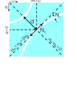
Figure 1: (Color online) Sketch of the phase-matching matrix $f_{m,q}$ in the space of the integer numbers $\{m,q\}$ corresponding to frequencies $\{\omega_{m},\omega_{q}\}$. In white are represented the regions of optimal phase-matching while in blue the unmatched regions.

The matrix $\mathcal{L}$ is the product of $f_{m,q}$ with the pump spectrum $\alpha_{m+q}$. As the last quantity is constant for $m+q=\mathrm{constant}$, the pump selects a portion of matrix $f_{m,q}$, roughly given by the intersection of $f_{m,q}$ with a straight band oriented along the direction $m+q=2m_{\max}$, where $m_{\max}$ corresponds to the maximum of the pump spectrum.

V.1 Analytical approach

When the pump spectrum is not very broad, the resulting nonzero matrix elements of $\mathcal{L}$ are confined within an “ellipse” whose principal axes are oriented along the directions $m+q=0$ and $m-q=0$. In this case one can forget the secondary maxima of the sinc function and use a Gaussian approximation for the phase-matching matrix:

$$f_{m,q}=e^{-\frac{1}{2}\left(\frac{m+q}{N_{1}}\right)^{2}}e^{-\frac{1}{2}\left(\frac{m-q}{N_{2}}\right)^{2}},$$ (62)

The form for $f_{m,q}$ follows from the approximations $\frac{\sin x}{x}\simeq e^{-\frac{x^{2}}{\eta_{1}}}$ and $\frac{\sin x^{2}}{x^{2}}\simeq e^{-\frac{x^{2}}{\eta_{2}}}$ Polish , where the parameters $\eta_{1}$ and $\eta_{2}$ can be opportunely chosen so that the results from the diagonalization of the coupling matrix obtained from (62) match optimally to the results of the numerical diagonalization of $\mathcal{L}_{m,q}$. By choosing them as $\eta_{1}=5$ and $\eta_{2}=12$, the following expressions for the widths $N_{1}$ and $N_{2}$ can be obtained:

$$N_{1} =\frac{\sqrt{5/2}}{\left|\beta_{1}\right|},$$ (63)

$$N_{2} =\frac{2\sqrt{3}}{\sqrt{\left|\beta_{2\mathrm{s}}\right|}}.$$ (64)

where the $\beta$ coefficients are the ones introduced in (23), (24), (25).

Let us assume in addition that the pump has a Gaussian spectrum centered at $2\omega_{0}$:

$$\alpha_{m}=\pi^{-\frac{1}{4}}N_{\mathrm{p}}^{-\frac{1}{2}}e^{-\frac{1}{2}\left(\frac{m}{N_{\mathrm{p}}}\right)^{2}}$$ (65)

where $\sum\left|\alpha_{m}\right|^{2}=1$ and $N_{\mathrm{p}}=\left(\Omega\tau_{\mathrm{p}}\right)^{-1}$ is a measure of the number of pump modes. The matrix elements $\mathcal{L}_{m,q}$ are then equal to:

$$\mathcal{L}_{m,q}=e^{-\frac{1}{2}\left(\frac{m+q}{N_{1}}\right)^{2}}e^{-\frac{1}{2}\left(\frac{m-q}{N_{2}}\right)^{2}}\frac{1}{\pi^{1/4}\sqrt{N_{\mathrm{p}}}}e^{-\frac{1}{2}\left(\frac{m+q}{N_{\mathrm{p}}}\right)^{2}}.$$ (66)

The Gaussian approximation (66) is correct as far as the interplay between the pump spectrum and the phase-matching is opportune. More quantitatively speaking, we have to demand that the two branches of the hyperbola in Fig. 1 are sufficiently separated each other, which corresponds to require that $d\gg N_{1}$ (we will consider $d\gtrsim 10N_{1}$), and the pump width is sufficiently smaller than the width of phase-matching function along the direction $m-q=0$, which corresponds to the condition $N_{\mathrm{p}}\lesssim N_{1}$. These conditions lead to the following bounds:

$$\frac{\beta_{1}^{2}}{\left|\beta_{2\mathrm{p}}-\frac{1}{2}\beta_{2\mathrm{s}}\right|}>20,\text{ }2\left|\beta_{1}\right|N_{\mathrm{p}}<1.$$

In terms of the crystal parameters and of the pump pulse duration these validity limits can be cast as

$$l >20\frac{\left|k_{\mathrm{p}}^{\prime\prime}-\frac{1}{2}k_{\mathrm{s}}^{\prime\prime}\right|}{\left(k_{\mathrm{p}}^{\prime}-k_{\mathrm{s}}^{\prime}\right)^{2}},$$ (67)

$$\tau_{\mathrm{p}} >\left|k_{\mathrm{p}}^{\prime}-k_{\mathrm{s}}^{\prime}\right|l.$$ (68)

For a BIBO crystal under typical conditions the above inequalities read $l>0.2\,\mu$m (hence it is not a serious condition) and $\tau_{\mathrm{p}}>400\,\mathrm{fs}\times l/\mathrm{mm}$. Hence, for a crystal length $l=1\,\mathrm{mm}$, $\tau_{\mathrm{p}}$ should be larger than $400$ fs in order that the Gaussian approximation is valid, while for $l=0.1$ mm the condition is met just for $\tau_{\mathrm{p}}>40$ fs. We note that condition (67) means that the pump duration should be longer than the temporal walk-off between signal and pump modes along their propagation inside the crystal.

The eigenvalues of such a matrix turn out to have a simple analytical expression at the continuous limit, i.e. when one can replace in (29) the sum by an integral, so that:

$$\Lambda_{k}L_{k}\left(m\right)=\int dq\mathcal{L}\left(m,q\right)L_{k}\left(q\right),$$ (69)

(note that we changed the notation from indices to arguments).

The eigenvalues are given by

$$\Lambda_{k}=\Lambda_{0}\rho^{k},$$ (70)

where

$$\Lambda_{0} =\pi^{1/4}\sqrt{2N_{\mathrm{p}}}\sqrt{\frac{\tau_{\mathrm{p}}^{2}}{\tau_{1}^{2}+\tau_{\mathrm{p}}^{2}}},$$ (71)

$$\rho =-1+2\sqrt{\frac{\tau_{2}^{2}}{\tau_{1}^{2}+\tau_{\mathrm{p}}^{2}}},$$ (72)

and

$$\tau_{1}=\frac{\left|k_{\mathrm{p}}^{\prime}-k_{\mathrm{s}}^{\prime}\right|l}{\sqrt{10}},\;\tau_{2}=\frac{\sqrt{\left|k_{\mathrm{s}}^{\prime\prime}\right|l\ }}{4\sqrt{3}},$$ (73)

$\Lambda_{0}$ and $\rho$ are given in the limit $\tau_{2}\ll\tau_{1}$, which holds unless the crystal length $l<0.1\mu$m; hence $\rho$ is very close to $-1$. Equation (70) corresponds then to an alternating geometric progression of ratio $\rho$, whose first element $\Lambda_{0}$ is positive.

The eigenvectors are similar to the well-known Hermite-Gauss $\mathrm{TEM}_{pq}$ transverse modes. They are given by

$$L_{k,m}=\frac{1}{\sqrt{k!2^{k}\sqrt{\pi}N_{\mathrm{s}}}}e^{-\frac{1}{2}\left(\frac{m}{N_{\mathrm{s}}}\right)^{2}}H_{k}\left(\frac{m}{N_{\mathrm{s}}}\right),$$ (74)

where $H_{k}$ is the Hermite polynomial of order $k$, and $N_{\mathrm{s}}$ is the number of signal modes. Hermite-Gauss functions being simply proportional to their Fourier transforms, their temporal shape is exactly the same as their spectral shape. The pulse duration of the zeroth mode, $\tau_{\mathrm{s}}$, is given by

$$\tau_{\mathrm{s}}^{2}=2\tau_{2}\sqrt{\tau_{1}^{2}+\tau_{\mathrm{p}}^{2}}.$$ (75)

Under typical conditions ordersofmagnitude the times $\tau_{1}$ and $\tau_{2}$ are on the order of $\tau_{1}\sim 100$ fs and $\tau_{2}\sim 5$ fs for a crystal length $l=1$ mm, and in general $\tau_{2}\ll\tau_{1}$ whenever $l\gtrsim 0.1\,\mu$m. Note that the condition (67) implies that $\tau_{\mathrm{p}}^{2}\gg\tau_{1}^{2}$, so that $\Lambda_{0}^{2}\simeq 2\sqrt{\pi}N_{\mathrm{p}}$.

We are then led to the important conclusion that, according to Eq. (31), the SPOPO threshold is roughly equal to the cw single mode threshold $P_{0}$ divided by the number of pump modes, and can be therefore very low. For example, if $N_{\mathrm{p}}=2\times 10^{4}$ (corresponding to $\tau_{\mathrm{p}}=100$ fs and a cavity length $L=2$ m) and considering the case already discussed (a $100\,\mu$m-thick BIBO based linear SPOPO pumped at $0.4\,\mu$m), we expect, for $T_{\mathrm{s}}=0.01$, a pump irradiance at threshold $P_{\text{{thr}}}^{\left(\text{{singly}}\right)}$ of $0.1\,\mathrm{kW}\,\mathrm{cm}^{-2}$, and an average pump power of $16\,\text{mW}$ for a typical pump beam radius of $70\,\mu$m.

V.2 Numerical approach

In the general case one must diagonalize numerically the $10^{5}\times 10^{5}$ matrix $\mathcal{L}$. The situation can be dramatically simplified from the computational viewpoint by noting that a scale transformation affecting the SPOPO parameters allows diagonalization of a much smaller matrix.

Let us now consider a set of parameters defined by

$$\beta_{1}^{\prime} =\kappa\beta_{1},\;\beta_{2\mathrm{p}}^{\prime}=\kappa^{2}\beta_{2\mathrm{p}},\;\beta_{2\mathrm{s}}^{\prime}=\kappa^{2}\beta_{2\mathrm{s}},$$ (76)

$$N_{\mathrm{p}}^{\prime} =\kappa^{-1}N_{\mathrm{p}}$$ (77)

with $\kappa$ a large and positive real number. Let us call $\mathcal{L}^{\prime}\left(m,q\right)$ the value of the matrix element with these new parameters. The form of the matrix coefficients $\mathcal{L}\left(m,q\right)$ when the phase mismatch coefficient $\phi_{m,q}$ has been replaced by its approximate value (22) implies that :

$$\mathcal{L}^{\prime}\left(m,q\right)=\sqrt{\kappa}\mathcal{L}\left(\kappa m,\kappa q\right).$$ (78)

Let us set the eigenvalue problem for $\mathcal{L}^{\prime}$:

$$\Lambda_{k}^{\prime}L_{k}^{\prime}\left(m\right)=\int\mathrm{d}q\mathcal{L}^{\prime}\left(m,q\right)L_{k}^{\prime}\left(q\right),$$ (79)

where we added a prime to denote the new eigen-elements. Using (78) and performing the change of variables $x=\kappa m,\;y=\kappa q$, one finds that:

$$\Lambda_{k} =\sqrt{\kappa}\Lambda_{k}^{\prime},$$ (80)

$$L_{k,m} =L_{k}^{\prime}\left(m/\kappa\right).$$ (81)

These two relations are very useful as they allow to compute numerically eigenvalues and eigenvectors of $\mathcal{L}$ in terms of the corresponding ones of much smaller matrix $\mathcal{L}^{\prime}$ because, according to (78), the support of $\mathcal{L}^{\prime}$ is much reduced as compared with that of $\mathcal{L}$. In any case the value for $\kappa$ must be chosen adequately in the sense that the diagonalization of the toy problem can be cast in the integral form (79) so as to keep $\mathcal{L}^{\prime}$ a smooth function of $\left(m,q\right)$.

As a by-product of the demonstration an interesting prediction on the influence of the cavity length can be drawn: consider that, given a SPOPO, we modify its length according to $L^{\prime}=\kappa^{-1}L$. This modifies the free spectral range as $\Omega^{\prime}=\kappa\Omega$ and the new SPOPO parameters relate to the old ones as in (76) and (77). Hence (79) leads to

$$\Lambda_{k}^{\prime}=\sqrt{L^{\prime}/L}\Lambda_{k}.$$ (82)

This is the case in particular for $\Lambda_{0}$ and the new pump threshold becomes $P_{\text{{thr}}}^{\prime}=(L/L^{\prime})P_{\text{{thr}}}$. Hence increasing the cavity length (and correspondingly decreasing the repetition rate) decreases the threshold accordingly.

VI Application of results in realistic cases

In this Section we discuss the threshold and squeezing properties of experimentally realizable SPOPOs. This study requires the numerical diagonalization of the matrix $\mathcal{L}$. We have explored many different configurations involving different pump pulse durations $\tau_{\mathrm{p}}$, different cavity lengths $L$, different crystal thicknesses $l$ and even different phase-matching conditions (critical and noncritical) that give rise to different dispersion properties. We have considered both BIBO and KNbO₃ crystals and have obtained similar results in the sense that the analytical approach given above describes very well what is numerically found in the region (67), no matter the particular values of the parameters. When that condition gets violated, deviations from the analytical result are obviously found but they affect mostly the behavior of the eigenvectors, not so much the one of the eigenvalues. As the analytical limit is the best also from an experimental viewpoint (there the eigenvectors are Hermite-Gauss modes, which can be reasonably easily produced experimentally) we consider here one case that clearly fulfills condition (67) with parameters compatible with the experimental setup that is currently under preparation. For the sake of completeness we also consider another one that “slightly” violates condition (67). We wish to remark that these cases are representative of what we have found in an exhaustive study. Finally, when condition (67) is more severely violated large deviations from the Hermite-Gauss case are observed that give rise in fact to new phenomena that deserve a study on their own and are not treated here.

The cases we discuss here correspond to collinear, degenerate type I critical phase-matching at $0.4\mu$m pumping of a BIBO crystal BIBO , obtained when the pump polarization is ordinary (parallel to the direction $Ox$) and that of the signal is extraordinary ($o\rightarrow e+e$). Using Sellmeier’s coefficients for BIBO we obtain that such phase-matching occurs at an angle $\theta=151^{\circ}$ between the direction $Oy$ and the direction of propagation of the pump (and the signal) beam, in agreement with experimBIBO . For this configuration we obtain the values for the dispersion parameters reported in Table 2. Also given in that table are the values of the free spectral range $\Omega$ and pump pulse duration $\tau_{\mathrm{p}}$ that will be used along this section. We shall assume a pump with Gaussian spectrum and centered at the phase-matched frequency $2\omega_{0}$. Finally we consider three different values of the crystal length:

case A $$\text{:}\;l=0.1\,\text{mm},$$

case B $$\text{:}\;l=0.5\,\text{mm},$$

case C $$\text{:}\;l=5\,\text{mm},$$

With all these values one can compute the phase mismatch angle $\phi$ in the second order dispersion approximation, see Eq. (22), and finally the matrix $\mathcal{L}$.

	$k^{\prime}$ (s m-1)	$k^{\prime\prime}$ (s2 m-1)
pump	$6.6537\times 10^{-9}$	$4.7248\times 10^{-25}$
signal	$6.2664\times 10^{-9}$	$1.6420\times 10^{-25}$

(a) BIBO dispersion parameters

$\Omega$ (MHz)	$\tau_{\mathrm{p}}$ (fs)
$2\pi\times 75$	$100$

(b) Pump parameters

Table 2: Dispersion parameters for BIBO crystal and pumping field.

Case A verifies well the condition (67), which reads here $\tau_{\mathrm{p}}>40$ fs. On the contrary cases B and C do not verify it, which now reads $\tau_{\mathrm{p}}>200$ fs and $\tau_{\mathrm{p}}>2000$ fs, respectively.

VI.1 Case A

In the next figure we show the matrix $\mathcal{L}$ corresponding to this case. Fig. 2 corresponds to the frequency (integer indexes) representation, which is the actual matrix to be diagonalized. Phase matching occurs in the lighter regions. Darker regions are highly phase-mismatched. Results of the numerical diagonalization, obtained as explained in Section V.2 by using a scale factor $\kappa=1000$, are shown in Figs. (3) and (4).

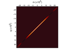
Figure 2: (Color online) Case A: $\mathcal{L}$ matrix.

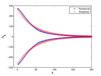
Figure 3: (Color online) Case A. Spectrum of eigenvalues. Comparison between the numerical and analytical solutions. Among about $10^{5}$ supermodes only a relatively small part ($\sim 40$) is dynamically significative.

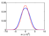
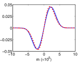
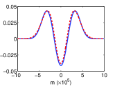
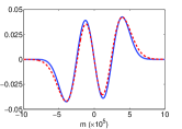
Figure 4: (Color online) Case A. Comparison between the numerical (solid blue line) and the analytical (dotted red line) solutions of the eigenvectors associated to the four highest $|\Lambda_{k}|$.

In the singly resonant case, a threshold of $W_{\mathrm{thr}}\simeq 29\,\text{mW}$ is readily obtained from Eq. (31) for the corresponding eigenvalue $\Lambda_{0}\simeq 270$, by considering a transmission factor of $T_{\mathrm{s}}=0.01$ and a beam waist of $70\,\mu$m. This results are in perfect agreement with the analytical value predictable by the expression Eq. (71). For a doubly resonant cavity this result has to be multiplied by means the correction factor that accounts for the geometry and is reported in Table 1.

From Eqs. (54) and (55) we can calculate also the noise reduction corresponding to the first four eigenvectors shown in Fig. 4 for a zero noise frequency. Evidently we are assuming to be able to master the spectral shape of the local oscillator in order to exactly match it to the supermode whose noise variance spectrum is to be measured. Nevertheless, the optimization of mode-matching between the local oscillator and a specific supermode can result a difficult task even when pulse shaping techniques are used. Let’s consider, then, the case where the best we can do is to deal with a local oscillator shaped as a Gauss-Hermite polynomial $e_{k,m}=\pi^{-1/4}N_{\mathrm{L}}^{-1/2}\mathrm{e}^{-\frac{1}{2}\left(m/N_{\mathrm{L}}\right)^{2}}\mathrm{e}^{i\phi_{\mathrm{L}}}H_{k}\left(m/N_{\mathrm{L}}\right)$, where $N_{\mathrm{L}}$ is the number of longitudinal modes of the local oscillator comb. In such situation the variances have to be evaluated using the general expression Eq. (IV.2.2), where the noise variance spectrum is given by the sum of all the supermodes noise variance spectra weighted by the mode matching parameters $d_{k}$, which describe how well each supermode projects on the local oscillator field. In Table 3 we compare the degree of squeezing measured in the situation of perfect mode-matching and the situation where the best local oscillator is Gauss-Hermite function of adjustable spectral width, for a pumping power $20\%$ below threshold (i.e. $r=0.9$).

$V_{k}$ (dB)	$k=0$	$k=1$	$k=2$	$k=3$
perfect	$-25.6$	$-24.9$	$-24.1$	$-23.3$
G-H	$-25.5$	$-24.8$	$-23.8$	$-22.6$

Table 3: Case A. Comparison between the noise variances evaluated, at $\omega=0$ and $r=0.9$, in the case of perfect mode matching of the LO with the supermodes corresponding to $k=0,1,2,3$ and the case where the LO is the Gauss-Hermite (G-H) function described by the spectral amplitudes $e_{k,m}$ and $N_{\mathrm{L}}=2.2\times 10^{5}$.

In the latter case, the minimum noise is obtained around $N_{\mathrm{L}}\simeq 2.2\times 10^{5}$. Such comparison evidences the fact that the differences between the two situations are small. Hence, the exact knowledge of the supermodes shape is not necessary and a good degree of mode matching can be obtained simply controlling the spectral width of a Gauss-Hermite local oscillator. Evidently this circumstance is verified as far as the condition for the Gaussian approximation of the coupling matrix is respected.However, the number of supermodes that present marked quantum characteristics results to be greater than four. By considering, in a qualitative way, that $-5\,\text{dB}$ is a still significative degree of squeezing, we found that all the supermodes corresponding to the first $45$ higher values of $|\Lambda_{k}|$ have variances smaller than the considered bound. This is an important result since it proves that SPOPOs are multi-mode sources of non-classical light.

VI.2 Case B

In the next figure we show the matrix $\mathcal{L}$ corresponding to this case. Fig. 5 corresponds to the frequency (integer indexes) representation, which is the actual matrix to be diagonalized. Phase matching occurs in the lighter regions, while darker regions are highly phase-mismatched.

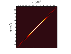
Figure 5: (Color online) Case B: $\mathcal{L}$ matrix.

Results of the numerical diagonalization, obtained as explained in Section V.2 by using a scale factor $\kappa=1000$, are shown in Figs. 6 and 7.

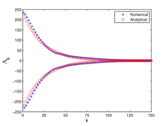
Figure 6: (Color online) Case B. Spectrum of eigenvalues. Comparison between the numerical and analytical solutions. Among about $10^{5}$ supermodes only a relatively small part ($\sim 23$) is dynamically significative.

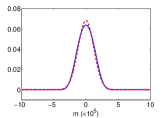
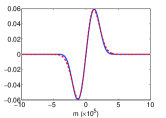
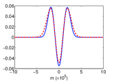
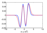
Figure 7: (Color online) Case B. Comparison between the numerical (solid blue line) and the analytical (dotted red line) solutions of the eigenvectors associated to the four highest $|\Lambda_{k}|$.

In the singly resonant case, a threshold of $W_{\mathrm{thr}}\simeq 1.5\,\text{mW}$ is readily obtained from Eq. (31) for the corresponding eigenvalue $\Lambda_{0}\simeq 235$, by considering a transmission of $T_{\mathrm{s}}=0.01$ and a beam waist of $70\,\mu$m. The threshold obtained from the analytical solution is about $1.6\,\text{mW}$, which is not too much different from the exact solution. Hence, even if the experimental situation considered here does not strictly verify the conditions for Gaussian approximation, we find still a good agreement between the numerical and the analytical predictions. A qualitative statement about the good agreement between the numerical and analytical solutions can be grounded also from the comparison between the eigenvalues shown in Fig. 7.

Assuming perfect mode matching, from Eqs. (54) and (55) we can calculate also the noise reduction corresponding to the first four eigenvectors shown in Fig. 7 at the carrying frequency and $20\%$ below threshold (i.e. $r=0.9$) and compare it to the general case where the local oscillator is described by the Gauss-Hermite spectral amplitudes $e_{k,m}$. In this case, the detection is optimized for a spectral width of about $N_{\mathrm{L}}\simeq 1.2\times 10^{5}$. The results are reported in Table 4.

$V_{k}$ (dB)	$k=0$	$k=1$	$k=2$	$k=3$
perfect	$-25.6$	$-24.1$	$-22.6$	$-21.0$
G-H	$-23.9$	$-20.8$	$-17.9$	$-15.0$

Table 4: Case B. Comparison between the noise variances evaluated, at $\omega=0$ and $r=0.9$, in the case of perfect mode matching of the LO with the supermodes corresponding to $k=0,1,2,3$ and the case where the LO is the Gauss-Hermite (G-H) function described by the spectral amplitudes $e_{k,m}$ and $N_{\mathrm{L}}=1.2\times 10^{5}$.

In this case, the amount of squeezing detected using a Gauss-Hermite local oscillator, despite of the optimization of its spectral width, is not as much as the perfect case, even if still significative. This result is a consequence of the fact that the situation now considered is slightly violating the bounds for the Gaussian approximation and, hence, the supermodes have spectral amplitudes that are no more characterized by Gauss-Hermite functions. Nevertheless, even if Gaussian approximation is not perfect, its prediction capability is still relevant.

Since we are interested to SOPOs as multi-mode sources for non-classical light, let’s consider the same qualitative argument we considered in the previous section. In this case about 23 supermodes present a degree of squeezing greater -5 dB. Despite the fact that, with respect to the 0.1mm-thick crystal, the number of supermodes that characterize the SPOPOs output is smaller, it can still be considered highly multi-mode.

VI.3 Case C

The last case we consider corresponds to a configuration that is strongly non-Gaussian. This can be directly observed by comparing the matrix $\mathcal{L}$ obtained in this case and reported in Fig. 8 with the matrices for cases A and B.

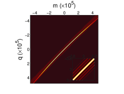
Figure 8: (Color online) Case C: $\mathcal{L}$ matrix. The inset is the magnification of the matrix around the phase-matched frequency corresponding to $m=0,\,q=0$.

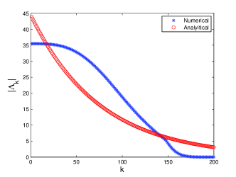
Figure 9: (Color online) Case B. Spectrum of eigenvalues. Comparison between the numerical and analytical solutions. Among about $10^{5}$ supermodes only a relatively small part ($\sim 125$) is dynamically significative.

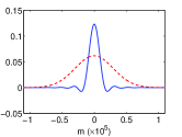
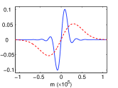
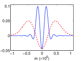
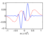
Figure 10: (Color online) Case C. Comparison between the numerical (solid blue line) and the analytical (dotted red line) solutions of the eigenvectors associated to the four highest $|\Lambda_{k}|$.

In fact, since the pump pulse duration $\tau_{\mathrm{p}}$ is much smaller than the temporal walk-off $|k^{\prime}_{\mathrm{p}}-k^{\prime}_{\mathrm{s}}|l$, in the space $\{m,q\}$, the pump bandwidth $N_{\mathrm{p}}$ is larger than the phase-matching bandwidth $N_{1}$ (see Fig. 1). Consequently, the pump selects not only the principal peak of the “sinc” function corresponding to the phase-matching matrix $f_{m,q}$, but also several secondary maxima. This has an important consequence for what concerns the eigenvectors and eigenvalues of $\mathcal{L}$, obtained as explained in Section V.2 by using a scale factor $\kappa=200$, that we report in Figs. 9 and 10.

In Fig. 9, the spectrum of the eigenvalues obtained from the analytical solution (70) (red circles) shows a great discrepancy with the eigenvalues obtained from numerical diagonalization of $\mathcal{L}$, as expected. In particular, the part of spectrum, corresponding about to the first $50$ eigenvalues, flatten around the critical value $\Lambda_{0}\simeq 36$, while the Gaussian approximation predicts always a geometric progression-like behavior with a critical eigenvalue $\Lambda^{\mathrm{Gauss}}_{0}\simeq 44$. In the same experimental configuration as previous cases (singly resonant cavity, transmission at signal frequencies of $T_{\mathrm{s}}=0.01$ and beam waist of $70\,\mu$m), a threshold of $W_{\mathrm{thr}}\simeq 0.67\,\text{mW}$ can be obtained from Eq. (31).

The result of a threshold higher than the one expected in the Gaussian approximation has a physical explanation. Since, for the time durations involved, the process of parametric down conversion can be considered almost instantaneous, for a mode-locked pumping field the peak power necessary to reach the oscillation threshold is the result of the coherent contribution of all its modes. This circumstance is formally expressed by the fact that the analytical expression for $\Lambda_{0}$ (see Eq. (70)) depends on the number of modes in the pump pulse $N_{\mathrm{p}}$. But, beyond the Gaussian limit, the fact that $N_{\mathrm{p}}\gg N_{1}$ implies that not all the $N_{\mathrm{p}}$ pump modes are equally phase-matched and, then, not all can optimally transfer energy towards the signal modes. The same phenomenon can be understood even in the temporal domain. In fact the quantity $|k^{\prime}_{\mathrm{p}}-k^{\prime}_{\mathrm{s}}|l$ corresponds to the temporal walk-off accumulated by the pump and signal pulses through a passage in the nonlinear crystal. When, in a non-Gaussian regime, the condition (67) is violated, the walk-off between pump and signal is bigger than the pump width $\tau_{\mathrm{p}}$ and the two field cannot optimally exchange energy all along the crystal length thus increasing the instantaneous peak power necessary to reach the oscillation.

On the other hand, in Fig. 10, the eigenvectors retrieved in the Gaussian approximation (74) do no more fit the numerical solutions, as expected. In fact, even if they still preserve a shape similar to Gauss-Hermite functions, they result to be shorter in the domain of frequencies and are affected by a small modulation of the spectral amplitude.

As the previous cases, we consider the quantum properties of the supermodes and compare the situation of perfect mode matching of the LO with that of a Gauss-Hermite LO. In this latter case the detection is optimized for a spectral width of about $N_{\mathrm{L}}\simeq 0.08\times 10^{5}$. The results are reported in Table 5 for the eigenvectors corresponding to the first four biggest $|\Lambda_{k}|$ .

$V_{k}$ (dB)	$k=0$	$k=1$	$k=2$	$k=3$
perfect	$-25.58$	$-25.58$	$-25.57$	$-25.57$
G-H	$-25.27$	$-24.28$	$-22.51$	$-20.22$

Table 5: Case C. Comparison between the noise variances evaluated, at $\omega=0$ and $r=0.9$, in the case of perfect mode matching of the LO with the supermodes corresponding to $k=0,1,2,3$ and the case where the LO is the Gauss-Hermite (G-H) function described by the spectral amplitudes $e_{k,m}$ and $N_{\mathrm{L}}=0.08\times 10^{5}$.

The fact that they are close to degeneracy (see Fig. 9) is reflected in an almost equal reduction of noise variances below the standard quantum limit. Despite the differences reported between the variances evaluated both by means of a perfectly mode matched and a Gauss-Hermite LO, a still significative degree of squeezing can be detected in realistic situations thus suggesting that the shaping of the LO is not a critical issue for the experimental configuration considered in this section. Actually, there is a larger set of supermodes the variances of which are all close to the value of the critical one. In particular, there are about $30$ supermodes that have variances comprised in $1$ dB, between $-24.6$ dB and $-25.6$ dB. Furthermore, by considering the number of supermodes that present a noise reduction bigger than $-5$ dB, one discovers that, this time, their number amounts to about $125$.

VI.4 Discussion on the influence of the crystal length

We have seen that even if the cases A and B do not verify at the same time the condition (67), the analytical solution obtained in the Gaussian approximation works quite well in both cases. Nevertheless, in spite of the fact that this condition gives an approximately good idea of the reliability of Gaussian approximation, it is interesting to study the passage from a perfectly Gaussian case to a non-Gaussian one trough a “gray” region where the differences between the two cases are not big.

Let us consider Eq. (70) in the limit of very large $l$. In such case, since from Eq. (73) $\tau_{1}\gg\tau_{\mathrm{p}}$, then $\Lambda_{0}$ asymptotically converges to:

$$\Lambda_{0}\simeq\pi^{1/4}\sqrt{20N_{\mathrm{p}}}\frac{\tau_{\mathrm{p}}}{|k^{\prime}_{\mathrm{p}}-k^{\prime}_{\mathrm{s}}|}\frac{1}{l}.$$ (83)

This expression indicates that the product $\Lambda_{0}\times l$ is constant for values of $l$ compatible with a non-Gaussian regime. In Figure 11, then, we report the values of this product as a function of the crystal thickness. For $l\lesssim 1$mm the analytical solution, as expected, is in good agreement with the numerical one, while for greater thicknesses the discrepancy is significative. Also this result is expected, since the analytical solution for the critical eigenvalue has not validity when the condition (67) is violated. On the other side, the fact that also the analytical solution reaches asymptotically, for increasing $l$, a plateau suggests a $1/l$-like behavior of $\Lambda_{0}$. The existence of such a plateau can be explained from the point of view of the evolution of the pump and signal pulses in the time domain. As discussed in the previous section, when the condition (67) is violated, the walk-off between pump and signal is bigger than the pump temporal width. As a consequence, the exchange of energy between the two fields is disadvantaged till a point where the threshold cannot change anymore even increasing the crystal length. Since, from Eqs. (20) and (31), $P_{\mathrm{thr}}\propto(\Lambda_{0}\times l)^{-2}$, for large values of $l$, then, also the product $\Lambda_{0}\times l$ reach a constant value, thus explaining the plateau in Fig. 11.

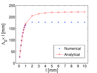
Figure 11: (Color online) Numerical and analytical curves for the product $\Lambda_{0}\times l$ versus the crystal length.

In the same way, one can explain the discrepancy observed between the two plateaux in Fig. 11. As already discussed in case C, in non-Gaussian configurations the pump bandwidth is larger than the phase-matching one, thus not all the pump modes are phase matched and not all of them contribute to the final value of the threshold. Therefore the number of pump modes actually involved is smaller than the nominal value $N_{\mathrm{p}}$ that should, then, be corrected.

From a quantum point of view, we have detailed in the previous sections the noise properties of the supermodes connected to the first four highest $\Lambda_{k}$ (see Tables 3, 4 and 5) and we calculated the number of supermodes showing a squeezing better than $-5$ dB for getting a qualitative indication about the “multimodicity” of the system prepared in a specific experimental configuration. These results can be appreciated in Fig. 12 where the noise variances of the supermodes that satisfy this criterium have been traced for the three cases previously discussed. The curve in the middle corresponds to case A ($l=0.1$mm), a Gaussian configuration. As the thickness of the crystal is increased to $l=0.5$ mm (case B) the condition (67) is violated but the Gaussian approximation is still good. This means that, even if the value of $\Lambda_{0}$ is decreasing (because we are reducing the number of pump modes that are phase-matched) the spectrum is still a geometric progression but with a smaller, in absolute value, common ratio (see $\rho$ in Eq. (70)) thus causing an overall decrease of the spectrum with respect to the case A. The consequence is a reduction of the number of supermodes with a squeezing greater than $-5$ dB as it results from the upper curve in Fig. 12 (red circles). Finally, when the crystal length is further increased to $l=5$mm (case C), we pass to a completely non-Gaussian configuration where the decrease of the critical eigenvalue $\Lambda_{0}$ (from $\sim 271$ for $l=0.1$ mm to $\sim 35$ for $l=5$ mm) causes a significative deformation of the spectrum and a non null set of eigenvalues flatten around $\Lambda_{0}$. In this case, since the degree of squeezing for each supermode depends on the ratio $|\Lambda_{k}/\Lambda_{0}|$ (see Eq. (56)), the amount of squeezing is globally increased as the lower curve (green diamonds) in Fig. 12 shows.

These results not only confirm that a SPOPO is a highly multi-mode device but also show another important quality: the malleability for controlling its “multimodicity”. We have seen, in fact, that one can just increase the thickness of the nonlinear crystal in order to improve the number of supermodes that play an important role from a quantum point of view.

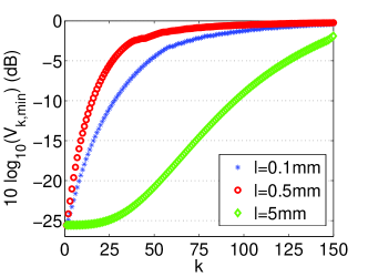
Figure 12: (Color online) Comparison between cases A ($l=0.1$mm, middle curve), B ($l=0.5$mm, upper curve) and C ($l=5$mm, lower curve). Noise variancese evaluated, at $\omega=0$ and $r=0.9$, in the case of perfect mode matching of the LO with the supermodes corresponding to the significative part of eigenspectrum $0\leq k\leq 150$. Among about $10^{5}$ supermodes only a relatively small part is significative from a quantum point of view. In particular, there are $45$, $23$ and $125$ supermodes, respectively, that are squeezed more than $-5$ dB.

In this paper we have presented a study of the eigenvalues and eigenvectors of the matrix $\mathcal{L}$ in function of the crystal length $l$. However, since both the pump pulse width and the crystal length are present in Eq. (67), notice that effects similar to those discussed in this section can be observed by playing with $\tau_{\mathrm{p}}$ and keeping constant $l$. In fact the passage from a Gaussian to a non-Gaussian configuration takes place when the pump bandwidth $N_{\mathrm{p}}$ becomes smaller than the phase-matching one $N_{1}$ and, clearly, this can be obtained keeping fixed the latter and increasing $\tau_{\mathrm{p}}$ (see Fig. 1). Eventually one could even fix $l$ and $\tau_{\mathrm{p}}$ and play with the group velocity mismatch by choosing different types of nonlinearities, but, experimentally, this could result in a stiffer malleability of the device.

VII Conclusion

In this paper, we have shown that both the dynamical and quantum noise properties of the SPOPO depend on the spectrum of eigenvalues $\Lambda_{k}$ of the linear coupling matrix $\mathcal{L}$. We have studied in detail this spectrum in various experimentally feasible configurations, using either an analytical approach in some simple limit cases, or a numerical approach in the general case. It turns out that among the roughly 100,000 eigenvalues, 99,900 or so are zero, and about a hundred are significantly different from zero and contribute to the quantum dynamics of the system. SPOPOs are therefore devices which produce simultaneously many highly squeezed vacuum modes. This property can be used to improve the performances of metrological methods using frequency combs, for example to perform ultra-accurate time transfer between remote clocks beyond the shot noise limit Lamine . In addition, it is well known that if one mixes by one way or another different squeezed modes, one gets strongly entangled states vanLoock . This is also the case here: we will show in a forthcoming publication that SPOPOs are indeed likely to generate various pairs of strongly entangled supermodes, as well as multipartite entangled states.

More generally, this paper is an example of the fact that, by using appropriately chosen pump spectra and phase matching curves, one can reach various eigenvalue spectra, and therefore tailor at will the quantum properties of the light generated by the optical system, which can be useful for example to generate interesting states for multidimensional quantum information processing.

VIII Appendix : Quantum model for a singly resonant SPOPO

We detail in this appendix the derivation of the Heisenberg equations in the case of a singly resonant degenerate type I SPOPO, i.e. when the signal field resonates inside the cavity, but not the pump field. We consider here the case of the linear Fabry-Perot cavity. The treatment of this case is more complex than the doubly resonant case usually considered in theoretical approaches as the pump field cannot be quantized inside the cavity.

The signal field inside the nonlinear crystal, which extends from $z=-l/2$ to $z=+l/2$, is written as

$$\hat{E}_{\mathrm{s}}\left(z,t\right)=i\sum\limits_{q}\mathcal{E}_{\mathrm{s},q}\sin\left(k_{\mathrm{s},q}z^{\prime}\right)\hat{s}_{q}\left(t\right)e^{-i\omega_{\mathrm{s},q}t}+\mathrm{H.c.},$$ (84)

where $z^{\prime}=z+L/2$, and $\mathcal{E}_{\mathrm{s},q}=\sqrt{\frac{\hbar\omega_{\mathrm{s},q}}{\varepsilon_{0}n\left(\omega_{\mathrm{s},q}\right)A_{\mathrm{s}}L}}$. On the contrary, the pump field is not affected by the cavity and hence it is given by a continuum of modes. We shall use the common approach of quantizing the pump field in a line of length $L_{\mathrm{p}}$ with periodic boundary conditions and, in the end of the calculations, we will make $L_{\mathrm{p}}\rightarrow\infty$. We thus write

$$\hat{E}_{\mathrm{p}}\left(z,t\right) = i\sum_{m}\mathcal{E}\left(\nu_{m}\right)e^{-i\nu_{m}t}\times$$ (85)

$$\times \left[\hat{p}_{m}^{\left(+\right)}\left(t\right)e^{i\kappa_{m}z}+\hat{p}_{m}^{\left(-\right)}\left(t\right)e^{-i\kappa_{m}z}\right]+$$

$$+ \mathrm{H.c.},$$

where the superscripts $\left(\pm\right)$ label the propagation direction. $\mathcal{E}\left(\nu_{m}\right)=\sqrt{\frac{\hbar\nu_{m}}{2\varepsilon_{0}A_{\mathrm{p}}L_{\mathrm{p}}n\left(\nu_{m}\right)}}$ are single photon field amplitudes. In the limit $L_{\mathrm{p}}\rightarrow\infty$ the frequencies $\nu_{m}$ are given by $\nu_{m}=m\frac{2\pi c}{L_{\mathrm{p}}}$, $m\in\mathbb{N}$, and the wavenumbers $\kappa_{m}=\frac{n\left(\nu_{m}\right)\nu_{m}}{c}$, with $n\left(\nu_{m}\right)$ the crystal refractive index. Note that we are writing the fields as a superposition of plane waves, but the treatment is still approximately valid for Gaussian beams as far as the thin crystal is placed at the (common) beam waist of pump and signal, and the Rayleigh lengths are much longer than the crystal length $l$. In such case $A_{\mathrm{f}}=\pi w_{\mathrm{f}}^{2}$ with $w_{\mathrm{f}}$ the corresponding beam radius.

The interaction Hamiltonian $\hat{H}_{\mathrm{I}}$ is calculated as usual as in (7). Inserting the expressions of the second order nonlinear electric polarizations, one obtains the following form of the interaction Hamiltonian, in which $\chi$ is the second order nonlinear susceptibility (whose dispersion is neglected):

$$\hat{H}_{\mathrm{I}}\left(t\right) = i\frac{\varepsilon_{0}\chi lA_{\mathrm{I}}}{2}\sum_{m}\sum_{q}\sum_{j}\mathcal{E}\left(\nu_{j}\right)\mathcal{E}_{\mathrm{s},m}\mathcal{E}_{\mathrm{s},q}F_{m,q}^{j}\times$$ (86)

$$\times \hat{s}_{m}^{{\dagger}}\left(t\right)\hat{s}_{q}^{{\dagger}}\left(t\right)\left[\hat{p}_{j}^{\left(+\right)}\left(t\right)+\hat{p}_{j}^{\left(-\right)}\left(t\right)\right]\times$$

$$\times e^{i\left(\omega_{\mathrm{s},m}+\omega_{\mathrm{s},q}-\nu_{j}\right)t}e^{-i\left(k_{\mathrm{s},m}+k_{\mathrm{s},q}\right)L/2}+$$

$$+ \mathrm{H.c.,}$$

where we defined the phase-mismatch factor

$$F_{m,q}^{j}=\frac{\sin\left[\left(\kappa_{j}-k_{\mathrm{s},m}-k_{\mathrm{s},q}\right)\frac{l}{2}\right]}{\left(\kappa_{j}-k_{\mathrm{s},m}-k_{\mathrm{s},q}\right)\frac{l}{2}}.$$ (87)

In (86) we dropped highly phase mismatched terms, as usual.

If we introduce new signal boson operators

$$\hat{s}_{m,\mathrm{new}}\left(t\right)=\hat{s}_{m}\left(t\right)e^{+ik_{\mathrm{s},m}L/2}$$ (88)

the interaction Hamiltonian becomes as (86) but without the exponential $e^{-i\left(k_{\mathrm{s},m}+k_{\mathrm{s},q}\right)L/2}$. In the following we will use the new operators but omit the superscript “$\mathrm{new}$” for simplicity.

From the previous expression of the hamiltonian, one can derive following Heisenberg equations governing the time evolution of the pump and signal operators:

$$\frac{d\hat{p}_{j}^{\left(\pm\right)}\left(t\right)}{dt} = -\frac{\varepsilon_{0}\chi lA_{\mathrm{I}}}{2\hbar}\sum_{m}\sum_{q}\mathcal{E}\left(\nu_{j}\right)\mathcal{E}_{\mathrm{s},m}\mathcal{E}_{\mathrm{s},q}F_{m,q}^{j}\times$$ (89)

$$\times \hat{s}_{m}\left(t\right)\hat{s}_{q}\left(t\right)e^{-i\left(\omega_{\mathrm{s},m}+\omega_{\mathrm{s},q}-\nu_{j}\right)t},$$

$$\frac{d\hat{s}_{m}\left(t\right)}{dt} = \frac{\varepsilon_{0}\chi lA_{\mathrm{I}}}{\hbar}\sum_{q}\sum_{j}\mathcal{E}\left(\nu_{j}\right)\mathcal{E}_{\mathrm{s},m}\mathcal{E}_{\mathrm{s},q}F_{m,q}^{j}\times$$ (90)

$$\times \hat{s}_{q}^{{\dagger}}\left(t\right)\left[\hat{p}_{j}^{\left(+\right)}\left(t\right)+\hat{p}_{j}^{\left(-\right)}\left(t\right)\right]\times$$

$$\times e^{i\left(\omega_{\mathrm{s},m}+\omega_{\mathrm{s},q}-\nu_{j}\right)t}.$$

The integration of the pump equations yields

$$\hat{p}_{j}^{\left(\pm\right)}\left(t\right) = \hat{p}_{\mathrm{free},j}^{\left(\pm\right)}-\frac{\varepsilon_{0}\chi lA_{\mathrm{I}}}{2\hbar}\sum_{m}\sum_{q}\mathcal{E}\left(\nu_{j}\right)\mathcal{E}_{\mathrm{s},m}\mathcal{E}_{\mathrm{s},q}F_{m,q}^{j}\times$$ (91)

$$\times \int\nolimits_{0}^{t}\mathrm{d}t^{\prime}\hat{s}_{m}\left(t^{\prime}\right)\hat{s}_{q}\left(t^{\prime}\right)e^{-i\left(\omega_{\mathrm{s},m}+\omega_{\mathrm{s},q}-\nu_{j}\right)t^{\prime}},$$

where $\hat{p}_{\mathrm{free},j}^{\left(\pm\right)}=\hat{p}_{j}^{\left(\pm\right)}\left(0\right)$ is the source-free part of the pump (the field impinging the nonlinear crystal).

Using the usual Wigner-Weisskopf approach, valid because the nonlinear interaction is assumed to be instantaneous, and using the approximation

$$\frac{\sin\left(\frac{\Omega}{2}t\right)}{\frac{\Omega}{2}}\simeq 2\pi\delta\left(\Omega\right),$$ (92)

we obtain a value of $\hat{p}_{j}^{\left(\pm\right)}\left(t\right)$ that one can then insert in Eq. (90):

$$\hat{p}_{j}^{\left(\pm\right)}\left(t\right) = \hat{p}_{\mathrm{free},j}^{\left(\pm\right)}\left(t\right)+$$ (93)

$$- \frac{\pi\varepsilon_{0}\chi A_{\mathrm{I}}l}{\hbar}\sum_{m}\sum_{q}\mathcal{E}\left(\nu_{j}\right)\mathcal{E}_{\mathrm{s},m}\mathcal{E}_{\mathrm{s},q}F_{m,q}^{j}\times$$

$$\times \hat{s}_{m}\left(t\right)\hat{s}_{q}\left(t\right)\delta\left(\omega_{\mathrm{s},m}+\omega_{\mathrm{s},q}-\nu_{j}\right),$$

We can now pass to the continuum limit. For that we define continuum pump operators in the following way:

$$\hat{p}_{\mathrm{free}}^{\left(\pm\right)}\left(\nu_{j}\right)=\sqrt{\frac{L_{\mathrm{p}}}{2\pi c}}\hat{p}_{\mathrm{free},j}^{\left(\pm\right)},$$ (94)

which verify

$$\left[\hat{p}_{\mathrm{free}}^{\left(\pm\right)}\left(\nu_{j}\right),\left[\hat{p}_{\mathrm{free}}^{\left(\pm\right)}\left(\nu_{k}\right)\right]^{{\dagger}}\right]=\frac{L_{\mathrm{p}}}{2\pi c}\delta_{j,k}\underset{L_{\mathrm{p}}\rightarrow\infty}{\longrightarrow}\delta\left(\nu_{j}-\nu_{k}\right).$$ (95)

Transforming sums into integrals, we obtain the following equation for the signal modes:

$$\frac{d\hat{s}_{m}\left(t\right)}{dt} = \frac{A_{\mathrm{I}}}{\sqrt{A_{\mathrm{p}}}}l\chi\sqrt{\frac{\varepsilon_{0}}{4\pi\hbar c}}\sum_{q}\mathcal{E}_{\mathrm{s},m}\mathcal{E}_{\mathrm{s},q}\hat{s}_{q}^{{\dagger}}\left(t\right)I_{m,q}^{\left(1\right)}+$$ (96)

$$- \frac{A_{\mathrm{I}}^{2}}{A_{\mathrm{p}}}\left(l\chi\right)^{2}\frac{\varepsilon_{0}}{2\hbar c}\sum_{n}\sum_{r}\sum_{q}\mathcal{E}_{\mathrm{s},m}\mathcal{E}_{\mathrm{s},q}\mathcal{E}_{\mathrm{s},n}\mathcal{E}_{\mathrm{s},r}\times$$

$$\times \hat{s}_{q}^{{\dagger}}\left(t\right)\hat{s}_{n}\left(t\right)\hat{s}_{r}\left(t\right)I_{m,q}^{\left(2\right)},$$

where

$$I_{m,q}^{\left(1\right)} = \int\mathrm{d}\nu\sqrt{\frac{\nu}{n\left(\nu\right)}}\frac{\sin\left[\left(k\left(\nu\right)-k_{\mathrm{s},m}-k_{\mathrm{s},q}\right)\frac{l}{2}\right]}{\left(k\left(\nu\right)-k_{\mathrm{s},m}-k_{\mathrm{s},q}\right)\frac{l}{2}}\times$$ (97)

$$\times \left[\hat{p}_{\mathrm{free}}^{\left(+\right)}\left(\nu\right)+\hat{p}_{\mathrm{free}}^{\left(-\right)}\left(\nu\right)\right]e^{i\left(\omega_{\mathrm{s},m}+\omega_{\mathrm{s},q}-\nu\right)t},$$

$$I_{m,q}^{\left(2\right)} = \int\mathrm{d}\nu\delta\left(\omega_{\mathrm{s},n}+\omega_{\mathrm{s},r}-\nu\right)\frac{\nu}{n\left(\nu\right)}\times$$ (98)

$$\times \frac{\sin\left[\left(k\left(\nu\right)-k_{\mathrm{s},m}-k_{\mathrm{s},q}\right)\frac{l}{2}\right]}{\left(k\left(\nu\right)-k_{\mathrm{s},m}-k_{\mathrm{s},q}\right)\frac{l}{2}}\times$$

$$\times \frac{\sin\left[\left(k\left(\nu\right)-k_{\mathrm{s},n}-k_{\mathrm{s},r}\right)\frac{l}{2}\right]}{\left(k\left(\nu\right)-k_{\mathrm{s},n}-k_{\mathrm{s},r}\right)\frac{l}{2}}\times$$

$$\times e^{i\left(\omega_{\mathrm{s},m}+\omega_{\mathrm{s},q}-\nu\right)t}.$$

In order to calculate the first integral, we write it as a sum over frequency intervals of width $\Omega$ and centered at frequencies $\omega_{\mathrm{p},r}=2\omega_{0}+r\Omega$, $r\in\mathbb{Z}$. Thus $I_{1}$ becomes

$$I_{m,q}^{\left(1\right)} \simeq e^{i\left(\omega_{\mathrm{s},m}+\omega_{\mathrm{s},q}\right)t}\sum_{r}\sqrt{\frac{\omega_{\mathrm{p},r}}{n\left(\omega_{\mathrm{p},r}\right)}}\times$$ (99)

$$\times \frac{\sin\left[\left(k_{\mathrm{p},r}-k_{\mathrm{s},m}-k_{\mathrm{s},q}\right)\frac{l}{2}\right]}{\left(k_{\mathrm{p},r}-k_{\mathrm{s},m}-k_{\mathrm{s},q}\right)\frac{l}{2}}\times$$

$$\times \int\nolimits_{r}\mathrm{d}\nu\left[\hat{p}_{\mathrm{free}}^{\left(+\right)}\left(\nu\right)+\hat{p}_{\mathrm{free}}^{\left(-\right)}\left(\nu\right)\right]e^{-i\nu t}$$

where $k_{\mathrm{p},r}=k\left(\omega_{\mathrm{p},r}\right)=k\left(2\omega_{0}+r\Omega\right)$.

We now define new pump operators

$$\sqrt{2\pi}e^{-i\omega_{\mathrm{p},r}t}\hat{p}_{\mathrm{in},r}^{\left(\pm\right)}\left(t\right)=\int\nolimits_{r}d\nu e^{-i\nu t}\hat{p}_{\mathrm{free}}^{\left(\pm\right)}\left(\nu\right).$$ (100)

which can be shown to verify the following property:

$$\left\langle\hat{p}_{\mathrm{in},r_{1}}^{\left(\pm\right)}\left(t_{1}\right)\left[\hat{p}_{\mathrm{in},r_{2}}^{\left(\pm\right)}\left(t_{2}\right)\right]^{{\dagger}}\right\rangle\simeq\delta_{r_{1},r_{2}}\delta\left(t_{1}-t_{2}\right).$$ (101)

$I_{m,q}^{\left(1\right)}$ now becomes

$$I_{m,q}^{\left(1\right)} \simeq \sqrt{2\pi}\sum_{r}\sqrt{\frac{\omega_{\mathrm{p},r}}{n\left(\omega_{\mathrm{p},r}\right)}}\frac{\sin\left[\left(k_{\mathrm{p},r}-k_{\mathrm{s},m}-k_{\mathrm{s},q}\right)\frac{l}{2}\right]}{\left(k_{\mathrm{p},r}-k_{\mathrm{s},m}-k_{\mathrm{s},q}\right)\frac{l}{2}}\times$$ (102)

$$\times e^{i\left(\omega_{\mathrm{s},m}+\omega_{\mathrm{s},q}-\omega_{\mathrm{p},r}\right)t}\left[\hat{p}_{\mathrm{in},r}^{\left(+\right)}\left(t\right)+\hat{p}_{\mathrm{in},r}^{\left(-\right)}\left(t\right)\right].$$

Retaining only slowly varying terms in the evolution, and including the losses of the optical cavity at rate $\gamma_{\mathrm{s}}$, one finally gets:

$$\frac{d\hat{s}_{m}\left(t\right)}{dt} = -\gamma_{\mathrm{s}}\hat{s}_{m}\left(t\right)+\sqrt{2\gamma_{\mathrm{s}}}\hat{s}_{\mathrm{in},m}\left(t\right)+$$ (103)

$$+ g\sum_{q}f_{m,q}\hat{s}_{q}^{{\dagger}}\left(t\right)\left[\hat{p}_{\mathrm{in},m+q}^{\left(+\right)}\left(t\right)+\hat{p}_{\mathrm{in},m+q}^{\left(-\right)}\left(t\right)\right]+$$

$$- g^{2}\sum_{n}\sum\limits_{q}f_{m,q}f_{n,m+q-n}\times$$

$$\times \hat{s}_{q}^{{\dagger}}\left(t\right)\hat{s}_{n}\left(t\right)\hat{s}_{m+q-n}\left(t\right),$$

where the coupling constant $g$ is given by

$$g=\chi\frac{A_{\mathrm{I}}}{A_{\mathrm{s}}\sqrt{A_{\mathrm{p}}}}\frac{l}{L}\left(\frac{\omega_{0}}{n_{0}}\right)^{3/2}\sqrt{\frac{\hbar}{\varepsilon_{0}c}}$$ (104)

and $\hat{s}_{\mathrm{in},m}\left(t\right)$ corresponds to the field at signal frequencies entering the cavity through the coupling mirror. When that input is coherent or vacuum, the case we consider, those “in” operators verify the following correlation

$$\left\langle\hat{s}_{\mathrm{in},m}\left(t\right)\hat{s}_{\mathrm{in},m^{\prime}}^{{\dagger}}\left(t^{\prime}\right)\right\rangle=\delta_{m,m^{\prime}}\delta\left(t-t^{\prime}\right),$$ (105)

and thus behave as $\hat{p}_{\mathrm{in},r}^{\left(\pm\right)}\left(t\right)$ (see Eq(101)).

Let us now consider the regime below the oscillation threshold : the signal modes are almost not excited and the double sum in (103) can be neglected. Also, the pump “in” fields can be approximated by their mean values as their fluctuation part gives rise to smaller terms, which are neglected for the same reasons as before. Hence, we have for a unidirectional pumping :

$$<\hat{p}_{\mathrm{in},m}^{\left(-\right)}\left(t\right)>=0\quad;\quad<\hat{p}_{\mathrm{in},m}^{\left(+\right)}\left(t\right)>=\sqrt{\frac{n_{0}A_{\mathrm{p}}P}{2\hbar\omega_{0}}}\alpha_{m},$$ (106)

$P$ being the average power per unit area of the modelocked pump laser and $\sum_{m}\left|\alpha_{m}\right|^{2}=1$. Eq. (106) is obtained by demanding that the pump field corresponding to the set $\left\{\hat{p}_{\mathrm{in},m}^{\left(+\right)}\left(t\right)\right\}$ equals the external pump field given by Eq. (1) inside the crystal. The linearized equations for the SPOPO below threshold finally become

$$\begin{split}\frac{d\hat{s}_{m}\left(t\right)}{dt}=&-\gamma_{\mathrm{s}}\hat{s}+\sqrt{2\gamma_{\mathrm{s}}}\hat{s}_{\mathrm{in},m}\left(t\right)+\\ &+\gamma_{\mathrm{s}}\sigma\sum\limits_{q}f_{m,q}\alpha_{m+q}\hat{s}_{q}^{{\dagger}}\left(t\right),\end{split}$$ (107)

where

$$\sigma=\sqrt{\frac{P}{P_{0}}}\quad;\quad P_{0}=\frac{\varepsilon_{0}c^{3}n_{0}^{2}T_{\mathrm{s}}^{2}}{32\left(\chi l\omega_{0}\right)^{2}}\left(\frac{A_{\mathrm{s}}}{A_{\mathrm{I}}}\right)^{2},$$ (108)

In conclusion, we have shown that the linearized equations (107) formally coincide with those of a doubly resonant SPOPO (Eq.(18)), the only difference being the exact value of $P_{0}$.

- (1) R. E. Slusher, P. Grangier, A. LaPorta, B. Yurke, and M. J. Potasek, Phys. Rev. Lett. 59, 2566 (1987).
- (2) R. M. Shelby and M. Rosenbluh, Appl. Phys. B 55, 226 (1992).
- (3) D. K. Serkland, M. M. Fejer, R. L. Byer, and Y. Yamamoto, Opt. Lett. 20, 1649 (1995).
- (4) K. Watanabe, Y. Ishida, Y. Yamamoto, H. Haus, Y. Lai, Phys. Rev. A 42, 5667 (1990).
- (5) M. Rosenbluh and R. Shelby, Phys. Rev. Lett. 66, 153 (1991).
- (6) S.R. Friberg, S. Machida. M.J. Werner, A. Levanon, T. Mukai, Phys. Rev. Lett. 77, 3775 (1996).
- (7) S. Schmitt, J. Ficker, M. Wolff, F. Konig, A. Sizmann, G. Leuchs, Phys. Rev. Lett. 81, 2446 (1998).
- (8) D. Krylov, K. Bergman, Opt. Lett. 23, 1390 (1998).
- (9) K. Hirosawa, H. Furumochi, A. Tada, F. Kannari, M. Takeoka, M. Sasaki, Phys. Rev. Lett. 94, 203601 (2005).
- (10) J. Sharping, M. Fiorentino, P. Kumar, Opt. Lett. 26, 367 (2001).
- (11) M. Fiorentino, J. Sharping, P. Kumar, A. Porzio, R. Windeler, Opt. Lett. 27, 649 (2002).
- (12) M. D. Levenson, R. M. Shelby, A. Aspect, M. Reid, and D. F. Walls, Phys. Rev. A 32, 1550 (1985).
- (13) R. M. Shelby, M. D. Levenson, S. H. Perlmutter, R. G. DeVoe, and D. F. Walls, Phys. Rev. Lett. 57, 691 (1986).
- (14) G. J. de Valcárcel, G. Patera, N. Treps, and C. Fabre, Phys. Rev. A 74, 061801(R) (2006).
- (15) J. A. Levenson, I. Abram, T. Rivera, P. Fayolle, J. C. Garreau, and P. Grangier, Phys. Rev. Lett. 70, 267 (1993).
- (16) A. Piskarskas, V. J. Smil’gyavichyus, and A. Umbrasas, Sov. Quantum Electron. 18, 155 (1988).
- (17) D. C. Edelstein, E. S. Wachman, and C. L. Tang, Appl. Phys. Lett. 54, 1728 (1989).
- (18) G. Mak, Q. Fu, and H. M. van Driel, Appl. Phys. Lett. 60, 542 (1992).
- (19) G. T. Maker and A. I. Ferguson, Appl. Phys. Lett 56, 1614 (1990).
- (20) M. Ebrahimzadeh, G. J. Hall, and A. I. Ferguson, Opt. Lett. 16, 1744 (1991).
- (21) M. J. McCarty and D. C. Hanna, Opt. Lett. 17, 402 (1992).
- (22) E. C. Cheung and J. M. Liu, J. Opt. Soc. Am. B 7, 1385 (1990) and 8, 1491 (1991).
- (23) M. J. McCarthy and D. C. Hanna, J. Opt. Soc. Am. B 10, 2180 (1993).
- (24) M. F. Becker, D. J. Kuizenga, D. W. Phillion, and A. E. Siegman, J. Appl. Phys. 45, 3996 (1974).
- (25) N. Forget, S. Bahbah, C. Drag, F. Bretenaker, M. Lef‘ebvre, and E. Rosencher, Actively mode-locked optical parametric oscillator, Opt. Lett. 31, 972 (2006).
- (26) R. S. Bennink and R. W. Boyd, Phys. Rev. A 66, 053815 (2002).
- (27) W. Wasilewski, A. I. Lvovsky, K. Banaszek, and C. Radzewicz, Phys. Rev. A 73, 063819 (2006); A. I. Lvovsky, W. Wasilewski, and K. Banaszek, J. Mod. Opt. 54, 721 (2007).
- (28) T. Opatrný, N. Korolkova, and G. Leuchs, Phys. Rev. A 66, 053813 (2002).
- (29) H. Huang, and J. H. Eberly, J. Mod. Opt. 40, 915 (1996).
- (30) C. K. Law, I. A. Walmsley, and J. H. Eberly, Phys. Rev. Lett. 84, 5304 (2000).
- (31) Samuel L. Braunstein, Phys. Rev. A 71, 055801 (2005).
- (32) N. C. Menicucci, S. T. Flammia, O. Pfister, Phys. Rev. Lett. 101, 130501 (2008).
- (33) , .
- (34) G. Patera, PhD Thesis, http://tel.archives-ouvertes.fr/tel-00404162/fr/
- (35) J. Seres, Appl. Phys. B 73, 705 (2001).
- (36) Should then the null eigenvalue at threshold would be instead of and the following analysis should be accordingly modified.
- (37) I. Pérez-Arjona, E. Roldán, and G. J. de Valcárcel, Europhys. Lett. 74, 247 (2006); Phys. Rev. A 75, 063802 (2007).
- (38) L. Knöll, W. Vogel, and D.-G. Welsch, Phys. Rev. A 43, 543 (1991).
- (39) Z. Jiang, C.-B. Huang, D. E. Leaird, and A. M. Weiner, Nature Photonics 1, 463 (2007).
- (40) C.-B. Huang, Z. Jiang, D. E. Leaird, J. Caraquitena, and A. M. Weiner, Laser&Photon. Rev. 2, 227 (2008).
- (41) V. R. Supradeepa, C.-B. Huang, D. E. Leaird, and A. M. Weiner, Opt. Express 16, 11878 (2008).
- (42) For typical crystals , and .
- (43) M. Ghotbi and M. Ebrahim-Zadeh, Opt. Express 12, 6002 (2004).
- (44) C. Navarrete-Benlloch, E. Roldán, and G. J. de Valcárcel, Phys. Rev. Lett. 100, 203601(2008).
- (45) C. Navarrete-Benlloch, G. J. de Valcárcel, and E. Roldán, Phys. Rev. A 79, 043820 (2009).
- (46) B. Lamine, C. Fabre, N. Treps, Phys. Rev. Lett. 101, 123601 (2008).
- (47) P. van Loock and S. L. Braunstein, Phys. Rev. Lett. 84, 3482 (2000).