Phenomenology and Cosmology of
Supersymmetric Grand Unified
Theories

Achilleas Vamvasakis

A thesis submitted for the degree of Doctor of Philosophy.
Supervised by Prof. George Lazarides.

Physics Division, School of Technology,
Aristotle University of Thessaloniki,
Thessaloniki 54124, Greece.

June 2009

Chapter 1 Preface

Until relatively recently, only before about thirty years ago, a physicist would divide contemporary knowledge in physics into two major, largely independent sectors, cosmology and particle physics. This division would reflect the two greatest scientific achievements of twentieth century theoretical physics, general relativity and quantum mechanics. And although we have not yet concluded, despite our great effort, in a unique verifiable theory, which would engage the above two in a single theoretical framework, interestingly enough, in recent years, particle physics and cosmology are found to be intimately connected in such an extent that we often include both of them under the general title “High Energy Physics” (HEP). Physicists in our days can hardly concoct particle physics without worrying about the cosmological consequences of their models and vice versa. This has been so mainly due to “inflation”, a model of cosmological evolution that has brought a change of paradigm in cosmology since 1981, when Alan Guth first published his idea.

This thesis belongs to this category of modern physics, this hybrid sector that incorporates research on the smallest and the largest, the particles and the universe. More specifically, we explore here the phenomenological and cosmological consequences of a specific model belonging to a class of models called “supersymmetric”. Supersymmetry (SUSY) is basically a symmetry, as its name suggests. But it is more than that. It is a new way of making physics, it is an ordering system within physics, it is a theory by itself. We will have more to say about supersymmetry in Chap. 2. To summarize, in this thesis we work with supersymmetry, a subcategory of particle physics, and with inflation, a subcategory of cosmology. The classification is rough since, as we explained, the boundary between particle physics and cosmology is in our days obscure. We have chosen a specific supersymmetric model, constructed some years ago to cope with a known particle physics problem, and explored its surprisingly rich inflationary cosmology.

In Chap. 2 we review some of the salient features of SUSY. We show how one can complement the Standard Model (SM) of particle physics to become compatible with SUSY and we deduce the minimal particle spectrum as it is expected to be if SUSY is realized in nature. Finally, we mention the case that SUSY becomes local, known as “supergravity” (SUGRA), and show its effect on the scalar potential of the theory, which is important for cosmology. This chapter is not intended to be a comprehensible introduction to SUSY but rather a “notation and conventions” chapter, included to make the reader familiar with the specific notation used in this thesis.

In Chap. 3 we give a short introduction to hybrid inflation, the kind of inflation most usually found in SUSY models. We begin by introducing the original model and then we go on to consider its natural realization within supersymmetric theories. Then, we describe in some detail two variants of SUSY hybrid inflation, namely “smooth” and “shifted” hybrid inflation. These models were introduced to solve the problem of monopole overproduction after the end of inflation in SUSY Grand Unified Theories (GUTs) that predict their existence. These variants of hybrid inflation also appear naturally in the cosmology of the model we investigate in this thesis.

Next, in Chap. 4, the specific model that will be the object of our survey, is introduced. We display the symmetries and describe the particle spectrum of the model. We exhibit the new lagrangian terms and give briefly the reasoning for their introduction. Finally, we shortly summarize the main property of the model, i.e. Yukawa quasi-unification. As the reader may notice, cosmology and inflation are not mentioned in this chapter. This reflects the fact that this model was first introduced to deal with a problem completely irrelevant to cosmology and it was only later realized that this model also contains interesting inflationary phenomenology.

In the following chapters we start unfolding the rich “inflationary variety” of the model. In Chap. 5 we describe the first cosmological scenario, named “new shifted” hybrid inflation. The name suggests its resemblance with standard shifted hybrid inflation, discussed in Sec. 3.5. Its novelty consists of the fact that, in contrast to the standard scenario, it is realized only by renormalizable interactions in the lagrangian. Of course, the mere fact that this inflationary scenario naturally arises from a specific viable particle physics model has its own value. We first present the scenario in global SUSY and summarize the calculation of radiative corrections, which are important for driving inflation. Then, we consider the changes that are brought to the model by making SUSY local, i.e. by including SUGRA corrections. In particular, it is shown that the scenario remains viable and that inclusion of SUGRA does not ruin inflation.

An other, qualitatively different, inflationary scenario, contained in the same particle physics model for a wide range of the parameter space, is presented in Chap. 6. It is called “semi-shifted” hybrid inflation and, as its name suggests, it also bears similarities to shifted hybrid inflation. However, in this case, the GUT gauge group is not completely broken to the SM gauge group during inflation but it carries an extra unbroken $\rm U(1)$ symmetry, which breaks immediately after inflation leading to the formation of cosmic strings. These strings can then contribute a small amount to the primordial curvature perturbation, giving thus a different cosmological situation. We first introduce the model in global SUSY and give some details of the calculation of the radiative corrections, which, as usual, are important for driving inflation. Then, we account for SUGRA corrections in the model and present the necessary framework for dealing with cosmic strings. Finally, we display our numerical results and show how this model can become compatible with gauge coupling constant unification.

In Chap. 7 we introduce the “new smooth” hybrid inflation model. Its name, as compared to “new shifted” hybrid inflation, suggests the resemblance of this model with smooth hybrid inflation, discussed in Sec. 3.4. Again, one interesting feature of the new model, in contrast to the old one, is its realization with the sole use of renormalizable interactions. However, this is not its only advantageous point. It turns out that the model provides us with one extra degree of freedom in fitting the cosmological data. Thus, in the case of global SUSY, we can achieve spectral indices much lower than the ones expected from the old model. Nevertheless, when we go on to consider the effect of SUGRA corrections, we will see that this degree of freedom is not enough, by itself, to account for a spectral index compatible with recent data. Thus, in Sec. 7.3, we explain how we can work this problem out, by including non-minimal terms in the Kähler potential.

An other feature of the “new smooth” model that can be exploited in our favor is the fact that the “new smooth” inflationary phase follows continuously from the standard hybrid phase, also contained in the same particle physics model under consideration. This guides us to the construction of a two-stage inflation model, which incorporates the two aforementioned consecutive stages and leads to increased freedom in fitting the cosmological data. This scenario, called “standard-smooth” hybrid inflation, is described in Chap. 8. We first present, as usual, the model in the global SUSY case. Then, we introduce SUGRA corrections and show that the predicted parameters can easily become compatible with the data, even in the case of minimal SUGRA. In the last section of this chapter, we again give a brief account of gauge coupling constant unification.

Finally, in Chap. 9, we summarize our conclusions from the survey of this model, which, if nothing else, it demonstrates the usefulness of relating cosmology with particle physics, as well as the wealth of new cosmological models that can emerge even from a single particle physics model.

Chapter 2 Supersymmetry and the Minimal Supersymmetric Standard Model

2.1 Introduction

The Standard Model (SM) of high energy physics, incorporating the Glashow-Weinberg-Salam model of electroweak interactions and the theory of Quantum Chromodynamics into a single theory, based on the semi-simple gauge group $G_{\rm SM}=\rm SU(3)_{c}\times SU(2)_{L}\times U(1)_{Y}$, has been proven a very successful framework for the description of particle physics experiments at energies up to a few hundreds GeV. Nevertheless, a number of theoretical reasons indicate that the SM may not be a correct theory at higher energies.

First of all, it is not a complete theory since it does not include gravity and any attempt so far towards this direction has failed. But, regardless of that purely theoretical reason, there are also hitches of a more “quantitative” nature. In particular, the so called “hierarchy problem”, establishes a huge discrepancy between the experimentally anticipated order of magnitude for the Higgs boson mass and its theoretical prediction. We know from the experiment that if the Higgs boson is responsible for the masses of all the particles in the SM, then its vacuum expectation value (VEV) is of the order $\langle H\rangle\sim 170\,\rm{GeV}$. Any reasonable symmetry breaking theory should contain a Higgs field with a mass between 100 and 1000 GeV if it is to predict the correct VEV for it without significant fine tuning. The problem is that such a low mass parameter is susceptible to large radiative corrections, which render it of the order of the unification scale of the theory. Since we are not willing to abandon the idea that the Higgs field is the origin of the masses of all the massive particles (this is the reason it was introduced in the first place), the only way for such a low mass parameter to be stable under radiative corrections is through some kind of special symmetry, able to fix the positive and negative parts of the radiative corrections to be exactly equal, so that they can cancel each other.

Physicists have come up with such a symmetry, called supersymmetry (SUSY), although in its early stages its development was not driven by the need for a solution to the hierarchy problem. Regarding this, it is quite impressive that a theory introduced for some theoretical reasons was later proven to also provide a solution to the hierarchy problem. Since radiative corrections include contributions from both boson and fermion loops, it is obvious that this symmetry should relate bosons and fermions in some profound way. Thus, the underlying transformation should transform bosons into fermions and vice versa. The operator $Q$ that generates these transformations will act on bosonic and fermionic states, turning them into fermionic and bosonic respectively, according to the scheme

$$Q|{\rm Boson}\rangle=|{\rm Fermion}\rangle,\qquad Q|{\rm Fermion}\rangle=|{\rm Boson}\rangle.$$ (2.1)

It is apparent from Eq. (2.1) that $Q$ is a complex spinor operator that carries spin angular momentum $1/2$. Thus, its hermitian conjugate, $Q^{\dagger}$, is also of the same nature. It can be proven [1] that, for realistic theories with chiral fermions, the generators $Q$ and $Q^{\dagger}$ must satisfy an algebra of commutation and anticommutation relations, called the SUSY algebra, of the form

$$\{Q_{\alpha},Q_{\dot{\beta}}^{\dagger}\}=2\sigma^{\mu}_{\alpha\dot{\alpha}}P_{\mu},$$ (2.2)

$$\{Q_{\alpha},Q_{\beta}\}=\{Q_{\dot{\alpha}}^{\dagger},Q_{\dot{\beta}}^{\dagger}\}=0,$$ (2.3)

$$[P^{\mu},Q_{\alpha}]=[P^{\mu},Q_{\dot{\alpha}}^{\dagger}]=0,$$ (2.4)

where $P^{\mu}$ is the generator of space-time translations, $\sigma^{\mu}$ represents the Pauli sigma matrices and $\alpha$, $\dot{\alpha}$, $\beta$, $\dot{\beta}$ are two component spinor indices (see e.g. [2]). The relations in Eqs. (2.2)-(2.4) can be used to show that each supermultiplet (i.e. each irreducible representation of the SUSY algebra) must contain an equal number of fermionic and bosonic degrees of freedom. From Eq. (2.4) it follows that the operator $P^{\mu}P_{\mu}$ commutes with $Q$ and $Q^{\dagger}$, which implies that particles in the same supermultiplet must have equal masses. The SUSY generators $Q$ and $Q^{\dagger}$ also commute with the generators of gauge transformations. Therefore, particles in the same supermultiplet must also reside in the same representation of the gauge group. Since we do not know of any such particles having equal masses, SUSY must be broken.

The solution to the hierarchy problem by supersymmetry is achieved by the cancellation of the quadratic divergencies, $\Lambda_{\rm UV}^{2}$, coming from the radiative corrections and this requires that the associated dimensionless couplings of fermion and boson superpartners, say schematically $\lambda_{S}$ and $\lambda_{f}$, are related, for example by a relation such as $\lambda_{S}=|\lambda_{f}|^{2}$ (see e.g. [2]). In fact, unbroken SUSY guarantees that the quadratic divergencies in scalar squared masses vanish to all orders in perturbation theory. But what about broken SUSY? Broken SUSY should still provide a solution to the hierarchy problem, which means that the relations between dimensionless couplings must be maintained. This leads to a very important consequence about broken SUSY, i.e. SUSY must be “softly” broken. This means that the effective lagrangian can be written in the form

$$\mathcal{L}=\mathcal{L}_{\rm SUSY}+\mathcal{L}_{\rm soft},$$ (2.5)

where $\mathcal{L}_{\rm SUSY}$ preserves supersymmetry and $\mathcal{L}_{\rm soft}$ violates supersymmetry but contains only mass terms and couplings with positive mass dimension (i.e. it does not contain Yukawa couplings). It turns out that there are plenty natural theoretical models for SUSY breaking with this property.

If the largest mass scale in the lagrangian $\mathcal{L}_{\rm soft}$ is denoted by $m_{\rm soft}$, then the SUSY breaking corrections to the Higgs $\rm mass^{2}$, $\Delta m_{H}^{2}$, should vanish in the limit $m_{\rm soft}\to 0$, so they can not be proportional to $\Lambda_{\rm UV}^{2}$. Furthermore, the corrections cannot go like $\Delta m_{H}^{2}\sim m_{\rm soft}\Lambda_{\rm UV}$, because the loop integrals always diverge either quadratically or logarithmically and never linearly with $\Lambda_{\rm UV}$. So, by dimensional analysis, they must be of the form

$$\Delta m_{H}^{2}=m_{\rm soft}^{2}\left[\frac{\lambda}{16\pi^{2}}\ln(\Lambda_{\rm UV}/m_{\rm soft})+\dots\right],$$ (2.6)

where the dots represent either terms that are independent of $\Lambda_{\rm UV}$ or higher order terms. Eq. (2.6) shows that the superpartner masses cannot be too big if we want to cure the hierarchy problem with broken SUSY and no fine tuning. This is the reason why we expect the consequences of supersymmetry to arise not very much higher than about $1\,\rm{TeV}$.

In the rest of this section we will briefly state a few things about the notation and the conventions used in this thesis. We will use two component Weyl spinor notation instead of four component Dirac spinors, as well because the description of SUSY in this context is much simpler, as because in SUSY models the minimal building blocks of matter are supermultiplets containing a single two component Weyl fermion.

A four component Dirac fermion $\Psi_{D}$ with mass $M$ is described by the lagrangian

$$\mathcal{L}_{\rm Dirac}=-i\bar{\Psi}_{D}\gamma^{\mu}\partial_{\mu}\Psi_{D}-M\bar{\Psi}_{D}\Psi_{D},$$ (2.7)

where the space-time metric is $\eta_{\mu\nu}=\operatorname{diag}(-1,1,1,1)$ and we use the following representation for the gamma and sigma matrices

$$\gamma_{\mu}=\left(\begin{array}[]{cc}0&\sigma_{\mu}\\ \bar{\sigma}_{\mu}&0\end{array}\right),\qquad\gamma_{5}=\left(\begin{array}[]{cc}1&0\\ 0&-1\end{array}\right),$$ (2.12)

$$\sigma_{0}=\bar{\sigma}_{0}=\left(\begin{array}[]{cc}1&0\\ 0&1\end{array}\right),\qquad\sigma_{1}=-\bar{\sigma}_{1}=\left(\begin{array}[]{cc}0&1\\ 1&0\end{array}\right),$$ (2.17)

$$\sigma_{2}=-\bar{\sigma}_{2}=\left(\begin{array}[]{cc}0&-i\\ i&0\end{array}\right),\qquad\sigma_{3}=-\bar{\sigma}_{3}=\left(\begin{array}[]{cc}1&0\\ 0&-1\end{array}\right).$$ (2.22)

In this bases, a four component Dirac spinor is written in terms of two component, complex, anticommuting Weyl spinors $\xi_{\alpha}$ and $\chi^{\dagger\dot{\alpha}}$ ($\alpha,\dot{\alpha}=1,2$), as

$$\Psi_{D}=\left(\begin{array}[]{c}\xi_{\alpha}\\[2.0pt] \chi^{\dagger\dot{\alpha}}\end{array}\right),\qquad\bar{\Psi}_{D}=\left(\begin{array}[]{cc}\chi^{\alpha}&\xi^{\dagger}_{\dot{\alpha}}\end{array}\right).$$ (2.23)

Here the notation is somewhat misleading since the indices $\alpha$ and $\dot{\alpha}$ do not appear on the left hand side. What this notation really means is that the undotted indices are used for the first two components of a Dirac spinor while the dotted are used for the last two ones. Note also that the location of an index (up or down) is important. The spinor indices are raised and lowered using the antisymmetric symbol $\epsilon^{\alpha\beta}$, with components $\epsilon^{12}=-\epsilon^{21}=-\epsilon_{12}=\epsilon_{21}=1$ and $\epsilon^{11}=\epsilon^{22}=\epsilon_{11}=\epsilon_{22}=0$. The spinor $\xi$ represents a left handed Weyl spinor while $\chi^{\dagger}$ is a right handed one. The notation implies that the hermitian conjugate of a left handed Weyl spinor is a right handed Weyl spinor and vice versa, $(\psi_{\alpha})^{\dagger}=\psi^{\dagger}_{\dot{\alpha}}$.

While $\xi$ and $\chi$ are anticommuting objects, the relation $\xi\chi=\chi\xi$ holds because of the abbreviation used here, which is $\xi\chi=\xi^{\alpha}\chi_{\alpha}=\xi^{\alpha}\epsilon_{\alpha\beta}\chi^{\beta}$. Likewise, $\xi^{\dagger}\chi^{\dagger}=\xi^{\dagger}_{\dot{\alpha}}\chi^{\dagger\dot{\alpha}}=(\xi\chi)^{*}$, the complex conjugate of $\xi\chi$. Similarly, $\xi^{\dagger}_{\dot{\alpha}}(\bar{\sigma}^{\mu})^{\dot{\alpha}\alpha}\chi_{\alpha}\equiv\xi^{\dagger}\bar{\sigma}^{\mu}\chi=-\chi\sigma^{\mu}\xi^{\dagger}=(\chi^{\dagger}\bar{\sigma}^{\mu}\xi)^{*}=-(\xi\sigma^{\mu}\chi^{\dagger})^{*}$. With these conventions, the Dirac lagrangian in Eq. (2.7) can be written as

$$\mathcal{L}_{\rm Dirac}=-i\xi^{\dagger}\bar{\sigma}^{\mu}\partial_{\mu}\xi-i\chi^{\dagger}\bar{\sigma}^{\mu}\partial_{\mu}\chi-M(\xi\chi+\xi^{\dagger}\chi^{\dagger}),$$ (2.24)

where we have dropped a total derivative piece, $i\partial_{\mu}(\chi^{\dagger}\bar{\sigma}^{\mu}\chi)$, which does not affect the action.

More generally any theory involving spin-$1/2$ fermions can always be written in terms of a collection of left handed Weyl spinors $\psi_{i}$ with the kinetic part of the lagrangian being

$$\mathcal{L}_{\rm kin}=-i\psi^{i\dagger}\bar{\sigma}^{\mu}\partial_{\mu}\psi_{i}.$$ (2.25)

For a Dirac fermion there is a different $\psi_{i}$ for its left handed part and for the hermitian conjugate of its right handed part. According to these general rules, we give names to the left handed spinors of the SM particles as follows

$$Q_{i} = (u,d),\;(c,s),\;(t,b),$$ (2.26)

$$\bar{u}_{i} = \bar{u},\;\bar{c},\;\bar{t},$$ (2.27)

$$\bar{d}_{i} = \bar{d},\;\bar{s},\;\bar{b},$$ (2.28)

$$L_{i} = (\nu_{e},e),\;(\nu_{\mu},\mu),\;(\nu_{\tau},\tau),$$ (2.29)

$$\bar{e}_{i} = \bar{e},\;\bar{\mu},\;\bar{\tau},$$ (2.30)

where $i$ is the family index and $Q_{i}$ and $L_{i}$ are doublets under the weak isospin symmetry $\rm SU(2)_{L}$ of $G_{\rm SM}$. The bars on the fields are part of their names and they do not indicate any kind of conjugation. In particular they are introduced to declare that the barred fields come from the conjugates of the right handed parts of the corresponding Dirac spinors. For example the Dirac spinor for the electron is written in terms of its two component left handed spinors as

$$\Psi_{e}=\left(\begin{array}[]{c}e\\ \bar{e}^{\dagger}\end{array}\right)=\left(\begin{array}[]{c}e_{L}\\ e_{R}\end{array}\right).$$ (2.31)

Note that the neutrinos are not part of a Dirac spinor in the SM. Of course, it is common in Grand Unified Theory (GUT) models to complete the picture with right handed parts for the neutrinos, which usually acquire large masses of the order of the GUT scale and explain the small left handed neutrino masses through the see-saw mechanism. Suppressing all color and weak isospin indices, the purely kinetic part of the SM fermion lagrangian is

$$\mathcal{L}^{\rm SM}_{\rm kin}=-iQ^{i\dagger}\bar{\sigma}^{\mu}\partial_{\mu}Q_{i}-i\bar{u}^{i\dagger}\bar{\sigma}^{\mu}\partial_{\mu}\bar{u}_{i}-i\bar{d}^{\,i\dagger}\bar{\sigma}^{\mu}\partial_{\mu}\bar{d}_{i}-iL^{i\dagger}\bar{\sigma}^{\mu}\partial_{\mu}L_{i}-i\bar{e}^{i\dagger}\bar{\sigma}^{\mu}\partial_{\mu}\bar{e}_{i}.$$ (2.32)

2.2 Supersymmetric lagrangians

Now, let us turn to the construction of supersymmetric lagrangians using the notation introduced in the previous section. The aim of the description here is to make the reader familiar with the notation and the style of this thesis and not to present a pedagogical introduction to supersymmetry. We begin by considering the simplest example of a supersymmetric theory in four dimensions.

The simplest possibility is a supermultiplet containing a single Weyl fermion (with two degrees of freedom) and two real scalars (each with one degree of freedom). Furthermore, one can assemble the two real scalars into a complex scalar field. This set of a two component Weyl fermion and a complex scalar field is called a “chiral” or “scalar” supermultiplet. The next simplest possibility for a supermultiplet contains a spin-$1$ vector boson, which is massless before the gauge symmetry breaking, so it has two bosonic degrees of freedom. Its superpartner is therefore a spin-$1/2$ Weyl fermion with two fermionic degrees of freedom. This collection of fields is called a “gauge” or “vector” supermultiplet. Gauge bosons transform as the adjoint representation of the gauge group, so their fermionic partners, called “gauginos”, must also transform according to the same representation. The adjoint representation of a gauge group is always its own conjugate, so these fermions have left and right handed components with the same transformation properties. This is in contrast with the fermions of the Standard Model which have left and right handed components belonging to different representations of the gauge group. Thus, in any supersymmetric extension of the SM all the known fermions must be included in chiral supermultiplets while all the known vector bosons will necessarily belong to gauge supermultiplets.

The simplest SUSY theory consists of a free chiral supermultiplet, containing a left handed Weyl fermion $\psi$ and a complex scalar $\phi$, with only kinetic terms, the simplified Wess-Zumino model [3]

$$\mathcal{L}=-\partial^{\mu}\phi^{*}\partial_{\mu}\phi-i\psi^{\dagger}\bar{\sigma}^{\mu}\partial_{\mu}\psi.$$ (2.33)

It can be proven (see e.g. [2]) that the action, $S=\int d^{4}x\;\mathcal{L}$, of this simple model is invariant under the SUSY transformations when the model is on-shell, i.e. when the equation of motion $\bar{\sigma}^{\mu}\partial_{\mu}\psi=0$, following from the action, is employed. Still, we would like supersymmetry to hold even off-shell.This can be fixed by a trick. We invent a new complex scalar field $F$ with no kinetic terms. Such a field is called auxiliary and it is not a real degree of freedom but only an object used to render the action invariant off-shell. The lagrangian density for $F$ is just $\mathcal{L}_{\rm aux}=F^{*}F$. The dimensions of $F$ are $\rm mass^{2}$ unlike ordinary scalar fields. The equation of motion for $F$ in the non-interacting theory is trivial, $F=0$, but it becomes non-trivial in the interacting case. In general, if we have a collection of chiral supermultiplets labelled by the index $i$, the free part of the lagrangian is written as

$$\mathcal{L}_{\rm chiral}^{\rm(free)}=-\partial^{\mu}\phi^{i*}\partial_{\mu}\phi_{i}-i\psi^{i\dagger}\bar{\sigma}^{\mu}\partial_{\mu}\psi_{i}+F^{i*}F_{i}.$$ (2.34)

The next thing is to do is to write down the lagrangian for a gauge supermultiplet. Consider a massless gauge boson $A_{\mu}^{a}$ and a corresponding set of Weyl fermion gauginos $\lambda^{a}_{\alpha}$, where the index $a$ runs over the adjoint representation of the gauge group. The on-shell degrees of freedom for $A_{\mu}^{a}$ and $\lambda^{a}_{\alpha}$ amount to two bosonic and two fermionic degrees of freedom for each $a$, as required by SUSY. However, the off-shell degrees of freedom do not much and we need to invent an auxiliary field, called $D^{a}$, in order to make the lagrangian supersymmetric. This field will also transform as the adjoint representation of the gauge group. Like the auxiliary field $F$, it has dimensions of $\rm mass^{2}$ and thus no kinetic terms. Without any further justification we write down the lagrangian for a gauge supermultiplet,

$$\mathcal{L}_{\rm gauge}^{\rm(free)}=-\frac{1}{2}F_{\mu\nu}^{a}F^{\mu\nu a}-i\lambda^{a\dagger}\bar{\sigma}^{\mu}D_{\mu}\lambda^{a}+\frac{1}{2}D^{a}D^{a},$$ (2.35)

where

$$F_{\mu\nu}^{a}=\partial_{\mu}A_{\nu}^{a}-\partial_{\nu}A_{\mu}^{a}-gf^{abc}A_{\mu}^{b}A_{\nu}^{c}$$ (2.36)

is the usual Yang-Mills field strength and

$$D_{\mu}\lambda^{a}=\partial_{\mu}\lambda^{a}-gf^{abc}A_{\mu}^{b}\lambda^{c}$$ (2.37)

is the covariant derivative for the gaugino field. It can be proven (see e.g. [2]) that this lagrangian is invariant under both gauge and SUSY transformations. Again, the equations of motion for the auxiliary fields are $D^{a}=0$, but this is no longer true in the interacting theory.

Up to now we have only dealt with free theories, not of much practical importance. We now turn to the description of interacting theories in the context of SUSY. Starting with the case of chiral supermultiplets, we will argue that the most general set of renormalizable interactions for these fields can be written as

$$\mathcal{L}_{\rm chiral}^{\rm(int)}=-\frac{1}{2}W^{ij}\psi_{i}\psi_{j}+W^{i}F_{i}+c.c.,$$ (2.38)

where $W^{ij}$ and $W^{i}$ are some functions of the scalar fields with dimensions of $\rm mass$ and $\rm mass^{2}$ respectively. It follows from Eq. (2.38) that, if the lagrangian is renormalizable, by dimensional analysis $W^{ij}$ and $W^{i}$ can not contain fermion or auxiliary fields. Furthermore, $W^{i}$ will be a quadratic polynomial and $W^{ij}$ linear in the fields $\phi_{i}$ and $\phi^{i*}$. Also, the lagrangian can not contain terms that are functions of the scalar fields only, because it can be shown that these terms do not respect SUSY. So, Eq. (2.38) is indeed the most general possibility. One can show, by requiring that the lagrangian is invariant under SUSY transformations, that $\partial W^{ij}/\partial\phi^{k*}=0$, i.e. the function $W^{ij}$ is analytic in the fields $\phi_{k}$. In addition, from Eq. (2.38) $W^{ij}$ can be taken to be symmetric under interchange of the indices $i,j$, so it can be written as

$$W^{ij}=M^{ij}+y^{ij\,k}\phi_{k},$$ (2.39)

where $M^{ij}$ represents a symmetric fermion mass matrix and $y^{ij\,k}$ the Yukawa couplings of a scalar with two fermions, totally symmetric under interchange of its indices. It is convenient to write

$$W^{ij}=\frac{\delta^{2}}{\delta\phi_{i}\delta\phi_{j}}\,W$$ (2.40)

introducing the “superpotential” $W$, given by

$$W=\frac{1}{2}M^{ij}\phi_{i}\phi_{j}+\frac{1}{6}\,y^{ij\,k}\phi_{i}\phi_{j}\phi_{k}.$$ (2.41)

$W$ is by no means a scalar potential in the ordinary sense, since it is not even real, but it is an analytic function of the complex variables $\phi_{i}$. Continuing to pursue the implications of the requirement that the lagrangian should respect SUSY and taking into account Eq. (2.40), one can prove that the function $W^{i}$ should be

$$W^{i}=\frac{\delta W}{\delta\phi_{i}}=M^{ij}\phi_{j}+\frac{1}{2}y^{ij\,k}\phi_{j}\phi_{k}.$$ (2.42)

Now it is clear why we have used for the two functions $W^{ij}$ and $W^{i}$ the same symbol.

To summarize the results in the case of chiral supermultiplets, we have found that the most general interactions can be determined simply by a single analytic function of the complex scalar fields, the superpotential $W$. The auxiliary field $F_{i}$ can be eliminated from the final form of the lagrangian using the classical equations of motion. From the lagrangian $\mathcal{L}_{\rm chiral}^{\rm(free)}+\mathcal{L}_{\rm chiral}^{\rm(int)}$, one finds $F_{i}=-W_{i}^{*}$ and $F^{i*}=-W^{i}$ and thus, the lagrangian for the chiral supermultiplets takes the form

$$\mathcal{L}_{\rm chiral}=-\partial^{\mu}\phi^{i*}\partial_{\mu}\phi_{i}-i\psi^{i\dagger}\bar{\sigma}^{\mu}\partial_{\mu}\psi_{i}-\frac{1}{2}\left(W^{ij}\psi_{i}\psi_{j}+h.c.\right)-W^{i}W_{i}^{*}.$$ (2.43)

It is clear from that equation that the scalar potential of the theory is completely determined by the superpotential and it reads

$$V(\phi,\phi^{*})=W^{i}W_{i}^{*} = M^{ji}M_{i\,l}^{*}\phi_{j}\phi^{\,l*}+\frac{1}{2}M^{ji}y_{i\,lm}^{*}\phi_{j}\phi^{\,l*}\phi^{m*}$$ (2.44)

$$+\frac{1}{2}M_{li}^{*}\,y^{ij\,k}\phi^{\,l*}\phi_{j}\phi_{k}+\frac{1}{4}y^{j\,ki}y_{i\,lm}^{*}\phi_{j}\phi_{k}\phi^{\,l*}\phi^{m*}$$

Of course, this is only the case when SUSY is unbroken. In broken SUSY there are also other terms in the scalar potential, which are responsible for SUSY breaking and which are not so strictly determined. The only requirement for these terms is that they should generate soft SUSY breaking, a restriction discussed earlier in Sec. 2.1. The supersymmetric scalar potential is automatically bounded from below. In fact, since it is a sum of squares of absolute values, it is always non-negative.

Finally let us consider supersymmetric gauge interactions. Suppose that the chiral supermultiplets transform under the gauge group in a representation $(T^{a})_{i}^{\phantom{i}j}$ satisfying $[T^{a},T^{b}]=if^{abc}T^{c}$, where $f^{abc}$ are the structure constants. Following well known techniques, to get a gauge invariant lagrangian we need to turn the ordinary derivatives into covariant derivatives, as

$$\partial_{\mu}\phi_{i}\to D_{\mu}\phi_{i}+igA_{\mu}^{a}(T^{a}\phi)_{i},\quad\partial_{\mu}\psi_{i}\to D_{\mu}\psi_{i}+igA_{\mu}^{a}(T^{a}\psi)_{i}.$$ (2.45)

Yet, this is not the end of the story since we have to consider whether there are any other interactions allowed by gauge invariance involving the gaugino and $D^{a}$ fields. Indeed, there are three such renormalizable terms, which read

$$(\phi^{*}T^{a}\psi)\lambda^{a},\qquad\lambda^{a\dagger}(\psi^{\dagger}T^{a}\phi)\qquad{\rm and}\qquad(\phi^{*}T^{a}\phi)D^{a}.$$ (2.46)

One can add these terms with arbitrary dimensionless coupling constants and demand that the whole lagrangian be real and invariant under SUSY transformations, up to a total divergence. This fixes the coefficients of these extra terms and the total lagrangian becomes

$$\mathcal{L}=\mathcal{L}_{\rm chiral}+\mathcal{L}_{\rm gauge}^{\rm(free)}-\sqrt{2}\,g\left[(\phi^{*}T^{a}\psi)\lambda^{a}+\lambda^{a\dagger}(\psi^{\dagger}T^{a}\phi)\right]+g(\phi^{*}T^{a}\phi)D^{a},$$ (2.47)

where $\mathcal{L}_{\rm chiral}$ is the lagrangian given in Eq. (2.43) but with ordinary derivatives replaced by gauge covariant derivatives and $\mathcal{L}_{\rm gauge}^{\rm(free)}$ is the lagrangian given in Eq. (2.35). From this lagrangian one can find the equations of motion for the $D^{a}$ fields, which are

$$D^{a}=-g(\phi^{*}T^{a}\phi).$$ (2.48)

Replacing $D^{a}$ in Eq. (2.47), one finds that the complete scalar potential is given by

$$V(\phi,\phi^{*})=F^{i*}F_{i}+\frac{1}{2}D^{a}D^{a}=W^{i}W_{i}^{*}+\frac{1}{2}\sum_{a}g_{a}^{2}(\phi^{*}T^{a}\phi)^{2}.$$ (2.49)

The two types of terms in this expression are called “F-terms” and “D-terms” respectively. The index $a$ in the gauge coupling constant $g_{a}$ is introduced to include the case that the gauge group has several distinct factors with different gauge couplings, as is the case with $G_{\rm SM}$. Note that the final scalar potential is always non-negative in a supersymmetric theory, since it is a sum of absolute squares. A very interesting and unique feature of unbroken SUSY is that the scalar potential is completely determined by the superpotential and the gauge interactions in the theory.

2.3 The MSSM superpotential

Given the supermultiplet content of the theory, the form of the superpotential is restricted by gauge invariance. In any given theory, only a subset of the couplings $M^{ij}$ and $y^{ij\,k}$ in Eq. (2.41) is allowed to be non-zero. In this section we will roughly describe the simplest possible supersymmetric extension of the SM, called Minimal Supersymmetric Standard Model (MSSM).

The field content of the theory is the one given in Eqs. (2.26)-(2.30), supplemented with their corresponding scalar superpartners and the usual gauge bosons of the SM along with their gaugino superpartners. In addition, one has to include a Higgs field, responsible for the breaking of the electroweak symmetry, accompanied by its fermionic superpartner, called the “higgsino”. In general, the nomenclature for a fermionic superpartner of a SM bosonic field is to append the ending “-ino” to its name. On the other hand, the names for the scalar superpartners of the SM fermions are constructed by prepending an “s-” to their names. For example, the superpartners of the quarks and leptons are generically called squarks and sleptons. In this thesis we will denote the scalar component of a chiral supermultiplet with the same symbol as the one used for the supermultiplet itself. The fermionic component of the supermultiplet, which is a two component Weyl spinor, will be denoted by $\psi_{x}$, where $x$ is the symbol used for the supermultiplet (and its scalar component). For example, the electron, which is the superpartner of the selectron $e$, is denoted by $\psi_{e}$. For a gauge supermultiplet, the gaugino corresponding to a gauge boson $A_{\mu}^{a}$ will be denoted by $\lambda^{a}$, with $T^{a}$ being the generator to which the gauge boson corresponds. In some circumstances, as e.g. in Table 2.1, the gaugino will be simply denoted by $\lambda_{X}$, if $X$ is the symbol used for the gauge boson.

Before writing down the full particle content of the MSSM, let us first say a few words about the Higgs boson. In the SM there was a need for only one such field with a scalar potential, responsible for giving mass to all the massive particles of the theory. Because of the structure of the superpotential, which is an analytic function of the scalar fields, in the MSSM one needs at least two scalar fields, with different transformation properties under $\rm U(1)_{Y}$ of $G_{\rm SM}$, to give masses to the up and down type quarks. In particular, as one can see from Table 2.1, one needs an $\rm SU(2)_{L}$ doublet with $Y=1/2$, denoted by $H_{u}$, to give mass to up type quarks and one with $Y=-1/2$, denoted by $H_{d}$, to give mass to down type quarks. This minimal choice for the Higgs bosons completes the particle spectrum of the MSSM, which is given collectively in Table 2.1 along with the transformation properties of the supermultiplets under $G_{\rm SM}$.

Table 2.1: The MSSM particle content

Names		SM particles	superpartners	$G_{\rm SM}$
quarks, squarks	$Q$	$(\psi_{u}\;\;\psi_{d}\,)$	$(u\;\;d\,)$	$(\bm{3},\bm{2},\frac{1}{6})$
($\times 3$ families)	$\bar{u}$	$\psi_{\bar{u}}$	$\bar{u}$	$(\bar{\bm{3}},\bm{1},-\frac{2}{3})$
	$\bar{d}$	$\psi_{\bar{d}}$	$\bar{d}$	$(\bar{\bm{3}},\bm{1},\frac{1}{3})$
leptons, sleptons	$L$	$(\psi_{\nu}\;\;\psi_{e})$	$(\nu\;\;e)$	$(\bm{1},\bm{2},-\frac{1}{2})$
($\times 3$ families)	$\bar{e}$	$\psi_{\bar{e}}$	$\bar{e}$	$(\bm{1},\bm{1},1)$
Higgs, higgsinos	$H_{u}$	$(\psi_{H_{u}^{+}}\;\;\psi_{H_{u}^{0}})$	$(H_{u}^{+}\;\;H_{u}^{0})$	$(\bm{1},\bm{2},+\frac{1}{2})$
	$H_{d}$	$(\psi_{H_{d}^{0}}\;\;\psi_{H_{d}^{-}})$	$(H_{d}^{0}\;\;H_{d}^{-})$	$(\bm{1},\bm{2},-\frac{1}{2})$
gluon, gluino	$g$	$g$	$\lambda_{g}$	$(\bm{8},\bm{1},0)$
W bosons, winos	$W$	$W^{\pm},W^{0}$	$\lambda_{W^{\pm}},\lambda_{W^{0}}$	$(\bm{1},\bm{3},0)$
B boson, bino	$B$	$B^{0}$	$\lambda_{B^{0}}$	$(\bm{1},\bm{1},0)$

Now that we have the full particle content of the theory, we are ready to write down the correct superpotential. Except for SUSY and gauge invariance, we will postulate that the superpotential respects an extra discrete symmetry, known as “$R$-parity” or “matter parity”. Define the operator

$$P_{M}=(-1)^{3(B-L)},$$ (2.50)

where $B$ and $L$ are the baryon and lepton number operators respectively. $R$-parity conservation consists of the principle that a term in the superpotential is allowed only if the product of $P_{M}$ for all of the fields in it is $+1$. This symmetry prevents terms in the superpotential, like $LL\bar{e}$, that respect gauge invariance but violate baryon and lepton number and lead to fast proton decay, a process strictly constrained by experiment. The superpotential for the MSSM, containing all the possible renormalizable terms that respect gauge invariance and $R$-parity, is

$$W_{\rm MSSM}=\bar{u}\,\bm{y}_{u}QH_{u}-\bar{d}\,\bm{y}_{d}\,QH_{d}-\bar{e}\,\bm{y}_{e}LH_{d}+\mu H_{u}H_{d},$$ (2.51)

where all the gauge and family indices are suppressed and the dimensionless parameters $\bm{y}_{u}$, $\bm{y}_{d}$ and $\bm{y}_{e}$ are $3\times 3$ matrices in family space. The “$\mu$-term”, as it is traditionally called, is the supersymmetric version of the Higgs boson mass and it can be written out analytically as $\mu(H_{u})_{\alpha}(H_{d})_{\beta}\epsilon^{\alpha\beta}$. The minus signs in Eq. (2.51) are chosen by convention so that when the matrices $\bm{y}_{u}$, $\bm{y}_{d}$ and $\bm{y}_{e}$ are diagonal, the terms that will give masses to the quarks and leptons after electroweak symmetry breaking appear in the superpotential with positive sign. For example, if we use the approximation $\bm{y}_{u}=\operatorname{diag}(0,0,y_{t})$, $\bm{y}_{d}=\operatorname{diag}(0,0,y_{b})$, $\bm{y}_{e}=\operatorname{diag}(0,0,y_{\tau})$, the superpotential reads

$$W_{\rm MSSM} = y_{t}\bar{t}tH_{u}^{0}+y_{b}\bar{b}bH_{d}^{0}+y_{\tau}\bar{\tau}\tau H_{d}^{0}-y_{t}\bar{t}bH_{u}^{+}-y_{b}\bar{b}tH_{d}^{-}-y_{\tau}\bar{\tau}\nu_{\tau}H_{d}^{-}$$ (2.52)

$$+\mu(H_{u}^{+}H_{d}^{-}-H_{u}^{0}H_{d}^{0}).$$

From the $\mu$-term of the superpotential, one can derive the mass terms of the Higgs scalar potential,

$$V_{\rm Higgs}\supset|\mu|^{2}\left(|H_{u}^{0}|^{2}+|H_{d}^{0}|^{2}+|H_{u}^{+}|^{2}+|H_{d}^{-}|^{2}\right).$$ (2.53)

Since Eq. (2.53) is positive definite, it is clear that we cannot understand electroweak symmetry breaking without including supersymmetry breaking soft terms, which can give negative $\rm mass^{2}$ terms. Thus, electroweak breaking is closely related with SUSY breaking. This leads to the infamous “$\mu$-problem”. As we have already pointed out in the introduction, we expect that $\mu$ should be roughly of order $10^{2}$ - $10^{3}\,\rm{GeV}$, in order to allow a Higgs VEV of order $170\,\rm{GeV}$ without too much fine tuning between $|\mu|^{2}$ and the negative $\rm mass^{2}$ terms coming from soft SUSY breaking terms. The problem is that, although, in contrast with the SM, $\mu$ will now be stable under radiative corrections if SUSY is softly broken, we do not have an explanation of why it should be so small in the first place compared to e.g. the Planck mass $M_{\rm P}$. In particular, the fact that it is roughly of the order $m_{\rm soft}$ (see Sec. 2.1) suggests that the $\mu$-term is probably not an independent parameter of the theory but is intimately connected with SUSY breaking. Several different solutions to this problem have been proposed. They all assume the parameter $\mu$ to be absent at tree level, usually by invoking some additional symmetry of the superpotential, as for example a $Z_{2}$ symmetry. The $\mu$-term is assumed to be dynamically generated at some stage of the history of the early universe by the VEV of some field. In this way, the value of the effective parameter $\mu$ need no longer be conceptually distinct from the mechanism of SUSY breaking. However, from the point of view of the MSSM, one can treat $\mu$ as an independent parameter.

2.4 Supergravity

Most symmetries in particle physics are realized as local symmetries, i.e. the parameters of a transformation are functions of the space-time point $x_{\mu}$. In particular, because the SUSY algebra contains the generator of translations $P_{\mu}$, we should consider translations that vary from point to point in space-time. Thus, we expect local SUSY to be a theory of general coordinate transformations of space-time, i.e. a theory of gravity. Therefore, the theory of local SUSY is referred to as supergravity (SUGRA) (for an introduction see e.g. [4]). In SUGRA, the spin-2 graviton has a spin-$3/2$ fermion superpartner, called the “gravitino”. As long as SUSY is unbroken, the graviton and the gravitino are both massless. Once SUSY is spontaneously broken, the gravitino acquires a mass, which is traditionally denoted by $m_{3/2}$.

SUGRA is a non-renormalizable theory and so it can only be thought of as a low energy approximation of some more complete theory, e.g. some string theory. For most practical purposes, the non-renormalizable terms can be neglected from the lagrangian, because they are suppressed by powers of $E/m_{\rm P}$, with $m_{\rm P}$ being the reduced Planck mass and $E$ represents the energy scales accessible to experiment. However, there are several reasons why one might be interested in non-renormalizable contributions to the lagrangian. For example, some very rare processes, like proton decay, can only be described by an effective lagrangian with non-renormalizable terms, since we know that the proton does not decay through renormalizable interactions. But, most importantly, the study of the early universe and cosmology are fields that SUGRA is expected to have significant consequences, as they refer to an era of high energy processes. Thus, in this section we will very roughly sketch some aspects of SUGRA and in particular its effect on the scalar potential.

Let us consider a supersymmetric theory containing some chiral and gauge supermultiplets. If one attempts to make SUSY local, it turns out that the part of the lagrangian containing terms up to two space-time derivatives is completely determined by specifying three independent functions of the scalar fields treated as complex variables. These are the superpotential $W(\phi_{i})$, the “Kähler potential” $K(\phi_{i},\phi^{i*})$ and the “gauge kinetic function” $f_{\alpha\beta}(\phi_{i})$. $W$ has dimensions $\rm mass^{3}$, $K$ has dimensions $\rm mass^{2}$ and $f_{\alpha\beta}$ is dimensionless. Unlike the superpotential, $K$ is real and analytic in the scalar fields. The Kähler potential does not appear in the renormalizable lagrangian for global SUSY because at tree level there is only one possibility for it, namely $K=\phi^{i*}\phi_{i}$. On the other hand, the gauge kinetic function is, like the superpotential, an analytic function of the scalar fields. The indices $\alpha$ and $\beta$ run over the adjoint representation of the gauge group and $f_{\alpha\beta}$ is symmetric under interchange of its two indices. In global SUSY, $f_{\alpha\beta}$ is independent of the fields and it equals the identity matrix divided by the square of the gauge coupling constant, $f_{\alpha\beta}=\delta_{\alpha\beta}/g^{2}$.

The whole lagrangian with up to two derivatives can now be written down in terms of these functions. To proceed, let us define one extra function, the “Kähler function”

$$G=K/m_{\rm P}^{2}+\ln(W/m_{\rm P}^{3})+\ln(W^{*}/m_{\rm P}^{3}).$$ (2.54)

From $G$ one can construct its derivatives with respect to the scalar fields and their complex conjugates, using the convention that a raised (lowered) index $i$ corresponds to derivation with respect to $\phi_{i}$ ($\phi^{i*}$), e.g. $G^{i}=\partial G/\partial\phi_{i}$, $G_{i}=\partial G/\partial\phi^{i*}$ and $G_{i}^{j}=\partial G/\partial\phi^{i*}\partial\phi_{j}$. Note that $G_{i}^{j}$, called the “Kähler metric”, depends only on $K$, since $G_{i}^{j}=K_{i}^{j}/m_{\rm P}^{2}$. The inverse of this matrix is denoted by $(G^{-1})_{i}^{j}$, so that $(G^{-1})_{i}^{k}G_{k}^{j}=\delta_{i}^{j}$. Similarly, the inverse of the matrix $K_{i}^{j}$ is denoted by $(K^{-1})_{i}^{j}$. In terms of these objects, the generalization of the F-term contribution to the scalar potential in SUGRA is given by (see e.g. [2])

$$V_{\rm SUGRA}^{F}=m_{\rm P}^{4}\;e^{G}\left[(G^{-1})_{i}^{j}\;G^{i}G_{j}-3\right].$$ (2.55)

Written in terms of the superpotential and the Kähler potential, this equation takes the form

$$V_{\rm SUGRA}^{F}=e^{K/m_{\rm P}^{2}}\left[(K^{-1})_{i}^{j}\;F^{i*}F_{j}-3|W|^{2}/m_{\rm P}^{2}\right],$$ (2.56)

with

$$F^{i*}=-(W^{i}+WK^{i}/m_{\rm P}^{2})\quad{\rm and}\quad F_{j}=-(W_{j}^{*}+W^{*}K_{j}/m_{\rm P}^{2}).$$ (2.57)

Now, if one assumes a “minimal” Kähler potential $K=\phi^{i*}\phi_{i}$, then $K_{i}^{j}=(K^{-1})_{i}^{j}=\delta_{i}^{j}$ and Eqs. (2.56)-(2.57), expanded to lowest order in $1/m_{\rm P}$, become $V_{\rm SUGRA}^{F}=F^{i*}F_{i}$, $F^{i*}=-W^{i}$ and $F_{i}=-W_{i}$, i.e. they take on their form in the global SUSY case. The D-term contribution to the scalar potential is given by

$$V_{\rm SUGRA}^{D}=\frac{1}{2}\operatorname{Re}f_{\alpha\beta}^{-1}\;\hat{D}^{\alpha}\hat{D}^{\beta},\quad{\rm with}\quad\hat{D}^{\alpha}=-K^{i}(T^{\alpha})_{i}^{\phantom{i}j}\phi_{j},$$ (2.58)

where $\operatorname{Re}f_{\alpha\beta}^{-1}$ is the inverse of the real part of the gauge kinetic function, viewed as a matrix. In the case of minimal Kähler potential and $f_{\alpha\beta}=\delta_{\alpha\beta}/g^{2}$, this just reproduces the result for the global SUSY case, i.e. $V_{\rm SUGRA}^{D}=1/2\,D^{\alpha}D^{\alpha}$. There are also many contributions to the lagrangian other than the scalar potential, which depend on the three functions $W$, $K$ and $f_{\alpha\beta}$, which we will not deal with here. The only thing that we will mention, in order to have a complete picture of the dynamics of a scalar field during inflation, is the form of the kinetic terms, which become

$$\mathcal{L}_{\rm SUGRA}^{\rm(kin)}=-K_{i}^{j}\;\partial^{\mu}\phi^{i*}\,\partial_{\mu}\phi_{j}.$$ (2.59)

It should be noted that, unlike the case of global SUSY, the scalar potential in SUGRA is not necessarily non-negative, because of the $-3$ term in Eq. (2.55).

Chapter 3 Hybrid inflation and extensions

3.1 Introduction

The next thing one needs to consider in order to proceed to the study of the early universe is, of course, cosmology. Early cosmology, soon after Einstein published his General Theory of Relativity, was haunted by the idea of a static universe, without any expansion or contraction. In contrast to this idea, Einstein’s equations kept predicting an expanding universe, which led him to introduce the famous cosmological constant in order to make them compatible with contemporary belief. But, when in 1929 Edwin Hubble formulated his law of expansion of the universe, after nearly a decade of observations, the picture changed radically, causing Einstein to make the legendary statement that the work on the cosmological constant was his greatest blunder. Hubble expansion, along with the later discovery of the cosmic microwave background radiation (CMBR) in 1964, established the hot big band (HBB) model as the standard cosmological model for the years to come. Today, the HBB model has been replaced by the theory of inflation which, although it constitutes a change of paradigm in cosmology, has kept many of the salient features of its predecessor.

Central and firm feature in all theories of modern cosmology has been the cosmological or Copernican principle, postulating that the universe is pretty much the same everywhere. The strongest evidence for this principle, that holds only on the largest scales of observation of the universe, is the observed isotropy of the CMBR. Mathematically, this principle is expressed by the notions of homogeneity and isotropy. Homogeneity is the statement that the metric is the same throughout the space. Isotropy applies at some specific point in space and states that space looks the same along all directions of observation through this point. Note that, if space is isotropic around one point and also homogeneous, then it will be isotropic around every point. Applying these notions to the metric one ends up with only one possible form for it, the Robertson-Walker metric (see e.g. [5])

$$ds^{2}=-dt^{2}+a^{2}(t)\left[\frac{dr^{2}}{1-kr^{2}}+r^{2}(d\theta^{2}+\sin^{2}\theta\,d\phi^{2})\right],$$ (3.1)

where $r$, $\phi$ and $\theta$ are “comoving” coordinates, which remain fixed for objects that have no other motion other than the general expansion of the universe. The parameter $k$ is the “scalar curvature” of the 3-space and $k=0$, $>0$ or $<0$ corresponds to flat, closed or open universe. The dimensionless parameter $a(t)$ is called the “scale factor” of the universe and describes the cosmological expansion.

Up to now, we have not made use of Einstein’s equations,

$$G_{\mu\nu}=8\pi GT_{\mu\nu},$$ (3.2)

where $G_{\mu\nu}=R_{\mu\nu}-1/2Rg_{\mu\nu}$ is the Einstein tensor, $R_{\mu\nu}$ and $R$ are the Ricci tensor and scalar, $T_{\mu\nu}$ is the energy-momentum tensor and $G=M_{\rm P}^{-2}$ is Newton’s constant. For a homogeneous and isotropic universe, the energy-momentum tensor takes the diagonal form $T_{\mu}^{\phantom{\mu}\nu}=T_{\mu\sigma}g^{\sigma\nu}=\operatorname{diag}(-\rho,p,p,p)$, where $\rho$ is the energy density of the universe and $p$ the pressure. With this form for the energy-momentum tensor, Einstein’s equations give

$$\frac{\ddot{a}}{a}=-\frac{4\pi G}{3}\,(\rho+3p),$$ (3.3)

$$\left(\frac{\dot{a}}{a}\right)^{2}=\frac{8\pi G}{3}\,\rho-\frac{k}{a^{2}},$$ (3.4)

where a dot represents a derivative with respect to the cosmic time $t$. Together, these two equations are known as the Friedmann equations and metrics of the form of Eq. (3.1) which obey these equations define Friedmann-Robertson-Walker (FRW) universes. From the Friedmann equations, or directly from conservation of energy and momentum $T_{\mu\phantom{\nu};\nu}^{\phantom{\mu}\nu}=0$, one obtains the continuity equation

$$\dot{\rho}=-3H(t)(\rho+p),$$ (3.5)

where the Hubble parameter $H(t)\equiv\dot{a}/a$ characterizes the rate of expansion of the universe. The value of the Hubble parameter at the present epoch is the Hubble constant, $H_{0}$. Another useful quantity is the density parameter, $\Omega=\rho/\rho_{c}=8\pi G\rho/3H^{2}$, where the critical density, $\rho_{c}=3H^{2}/8\pi G$, is the energy density corresponding to a flat universe. Thus, $\Omega=1$, $>1$ or $<1$ corresponds to flat, closed or open universe.

It is possible to solve the Friedmann equations in a number of simple cases. To do that, one needs an extra condition, known as the equation of state, which is a relation between $\rho$ and $p$ that depends on the form of the energy that the universe contains. Most of the perfect fluids relevant to cosmology obey the simple equation of state $\rho+p=\gamma\rho$, where $\gamma$ is a constant independent of time. With this assumption, Eq. (3.5) becomes $\rho\propto a^{-3\gamma}$ and substituting in Eq. (3.4), in the case of a flat universe ($k=0$), we obtain

$$a(t)=a_{0}(t/t_{0})^{2/3\gamma},$$ (3.6)

where $a_{0}$ is the scale factor at a cosmic time $t=t_{0}$. It is common to take $t_{0}$ to represent the present time and define $a_{0}=1$. For a universe dominated by pressureless matter we have $p=0$ and thus $\gamma=1$. In the case of a radiation dominated universe, $p=\rho/3$ and $\gamma=4/3$. So, for a matter dominated universe we get the expansion law $a(t)=(t/t_{0})^{2/3}$, while for a radiation dominated universe we get $a(t)=(t/t_{0})^{1/2}$. Both of these solutions (and many others) predict that at time $t\to 0$, $a(t)\to 0$ and the energy density of the universe becomes infinite. This particular time instance $t=0$, had been considered by many physicists, although outside the validity of any real knowledge regarding that instance, to represent the creation of everything, including space-time itself, a process called the Big Bang. These solutions, along with their observational confirmation by Hubble, signify the beginning of the HBB era.

The HBB cosmological model achieved many great successes in the explanation of observations, such as the Hubble expansion, the existence of the CMBR and the abundances of light elements, which were formed during primordial nucleosynthesis. But it also came up against a number of shortcomings, such as the horizon and flatness problems and the magnetic monopole problem, when it is combined with GUTs that predict their existence. The horizon problem is the difficulty in explaining the isotropy of the CMBR, since it seems to come from regions of the sky that have never communicated causally in the past. The flatness problem consists of the fact that the energy density of the observable universe is at present very close to its critical energy density, so that, at the beginning of its evolution, $\Omega$ should have been inexplicably close to 1. Also, combined with GUTs that predict the existence of heavy magnetic monopoles, the HBB model leads to a cosmological catastrophe due to the overproduction of these monopoles. Finally, even if one takes the isotropy of the CMBR for granted, there is no explanation of the observed temperature fluctuations in it, or of the origin of the small density perturbations required for structure formation.

Inflation came as a solution to these problems [6]. The main idea underlying all versions of the inflationary universe scenario is that, in the very early stages of its evolution, the universe fell in a metastable, vacuum-like state with high energy density (for an introduction see e.g. [7, 8]). In such a state $\rho={\rm const.}$ and Eq. (3.5) gives $p=-\rho$. Then, from Eq. (3.4) with $k=0$, which corresponds to a flat universe as observations suggest, one gets

$$a(t)\propto e^{Ht},\quad H=\sqrt{\frac{8\pi G}{3}\,\rho},$$ (3.7)

i.e. the universe experiences an exponential expansion. Inflation ends when the universe leaves this metastable state, either by tunnelling out of it, or by slow rolling towards a critical point, depending on the model. It is assumed that after inflation, during which the universe has cooled down, reheating occurs and the universe continues its evolution according to the HBB model.

To briefly describe the salient properties of inflation, consider a real scalar field $\phi$ whose evolution is driven by the lagrangian density

$$\mathcal{L}=\frac{1}{2}\,\partial_{\mu}\phi\,\partial^{\mu}\phi-V(\phi),$$ (3.8)

where $V(\phi)$ is the potential energy density, which we assume to be quite flat near some point $\phi=\phi_{0}$. The energy-momentum tensor is found to be

$$T_{\mu}^{\phantom{\mu}\nu}=-\partial_{\mu}\phi\,\partial^{\nu}\phi+\delta_{\mu}^{\phantom{\mu}\nu}\left(\frac{1}{2}\,\partial_{\lambda}\phi\,\partial^{\lambda}\phi-V(\phi)\right).$$ (3.9)

Now, if we assume that there is a large region in space where the field $\phi$ is essentially homogeneous with a value near $\phi=\phi_{0}$, which changes very slowly with time due to the flatness of the potential, then the energy-momentum tensor takes the form $T_{\mu}^{\phantom{\mu}\nu}\simeq-V_{0}\delta_{\mu}^{\phantom{\mu}\nu}$, where $V_{0}=V(\phi_{0})$. This means that $\rho\simeq-p\simeq V_{0}$ and the conditions for an exponential expansion of the scale factor are fulfilled. The equation of motion of the homogeneous field $\phi$, derived from the lagrangian, reads

$$\ddot{\phi}+3H\dot{\phi}+V^{\prime}(\phi)=0,$$ (3.10)

where a dot represents the derivative $d/dt$, while a prime represents $d/d\phi$. Inflation is by definition the situation where the “kinetic” term $\ddot{\phi}$ is subdominant to the “friction” term $3H\dot{\phi}$ and Eq. (3.10) reduces to the inflationary equation

$$3H\dot{\phi}=-V^{\prime}(\phi).$$ (3.11)

The conditions for the validity of the inflationary equation can be summarized in the form of restrictions imposed to the two slow roll parameters, $\eta$ and $\epsilon$, as (see e.g. [8])

$$|\eta|\equiv m_{\rm P}^{2}\left|\frac{V^{\prime\prime}(\phi)}{V(\phi)}\right|\leq 1\quad,\quad\epsilon\equiv\frac{m_{\rm P}^{2}}{2}\left(\frac{V^{\prime}(\phi)}{V(\phi)}\right)^{2}\leq 1.$$ (3.12)

The end of the slow roll occurs when either of these inequalities is saturated. The exponential expansion of the universe during inflation can be measured by the number of the “e-foldings”, defined as the logarithmic growth of the scale factor between an initial time $t_{i}$ and a final time $t_{f}$,

$$N\equiv\ln\frac{a(t_{f})}{a(t_{i})}=\int_{t_{i}}^{t_{f}}H\,dt=\frac{1}{m_{\rm P}^{2}}\int_{\phi_{f}}^{\phi_{i}}\frac{V(\phi)}{V^{\prime}(\phi)}\,d\phi.$$ (3.13)

The great success of the inflationary cosmological model is that for $N\gtrsim 55$ all three problems of the HBB model mentioned above can be simultaneously solved (see e.g. [8]). Furthermore, inflation can explain the origin of the density perturbations required for structure formation in the universe. To understand this, one should note that an exponentially expanding space, called “de Sitter” space, can be considered as a black hole turned inside out, i.e. a black hole that surrounds the space from all sides. Then, exactly as in a black hole, there are quantum fluctuations governed by the equivalent Hawking temperature $T_{H}=H/2\pi$. Skipping all the details, the power spectrum of the primordial curvature perturbation at a scale $k_{0}$ can be approximated by (see e.g. [9])

$$P_{\mathcal{R}}^{1/2}\simeq\frac{1}{2\pi\sqrt{3}}\,\frac{V^{3/2}(\phi_{Q})}{m_{\rm P}^{3}V^{\prime}(\phi_{Q})},$$ (3.14)

where $\phi_{Q}$ is the value of the inflaton field when the scale $k_{0}$ crossed outside the inflationary horizon. This curvature perturbation is not the same for all length scales. The running of $P_{\mathcal{R}}^{1/2}$ with respect to $k$ is governed by a power law, with $k$ raised to an exponent called the “spectral index” $n_{\rm s}$. In addition, the perturbations may also have a significant “tensor” component, measured by the “tensor to scalar ratio” $r$. The spectral index, the tensor to scalar ratio and the running of the spectral index $dn_{\rm s}/d\ln k$, in the slow roll approximation, are given by (see e.g. [9])

$$n_{\rm s}\simeq 1+2\eta-6\epsilon,\quad r\simeq 16\epsilon,\quad\frac{dn_{\rm s}}{d\ln k}\simeq 16\epsilon\eta-24\epsilon^{2}-2\xi^{2},$$ (3.15)

where

$$\xi^{2}=m_{\rm P}^{4}\frac{V^{\prime}V^{\prime\prime\prime}}{V^{2}}$$ (3.16)

is the third slow roll parameter. By measuring various properties of the CMBR one can extract experimental values for $P_{\mathcal{R}}^{1/2}$, $n_{\rm s}$, $dn_{\rm s}/d\ln k$ and $r$ and compare the corresponding theoretical values with them. In order for a specific model to be realistic, it should predict values for the above parameters that lie within the experimental limits of the observed values.

Inflation is the most successful cosmological model so far and it is certainly the most promising, not only because of its success in explaining the shortcomings of the HBB model, but also because it has provided us with an unprecedented way to link cosmology and particle physics and with the ability to confront particle physics theories with cosmological observations. Yet, we are still very far from deciding which is the right model that describes best the realization of inflation in the universe. Many models have been proposed, each with different appealing characteristics. Among them, hybrid inflation is one of the most prevalent, often making its appearance spontaneously in particle physics models. In the sections that follow, we will briefly describe the original model and some of its most successful extensions within the context of SUSY.

3.2 The standard non-supersymmetric version

Standard hybrid inflation was initially proposed by Linde [10] in an attempt to construct new inflationary models by making the hybrids of some known ones, such as “chaotic” and “new” inflation. Hybrid inflation helped to solve some of the problems of the old models and turned out to be a very fruitful arena for inflationary model building. The idea is to use two real scalar fields $\chi$ and $\sigma$, of which $\chi$ provides the vacuum energy density that drives inflation and $\sigma$ is the slowly varying inflaton field. Inflation ends by a rapid rolling of the field $\chi$, called “waterfall”, triggered by the slow rolling of the field $\sigma$, when the latter reaches a critical value $\sigma_{c}$.

The scalar potential of the original model is of the form (for a review see e.g. [8])

$$V(\chi,\sigma)=\kappa^{2}\left(M^{2}-\frac{\chi^{2}}{4}\right)^{2}+\frac{\lambda^{2}}{4}\chi^{2}\sigma^{2}+\frac{m^{2}}{2}\,\sigma^{2},$$ (3.17)

where $\kappa$, $\lambda$ are dimensionless parameters and $M$, $m$ are mass parameters. This potential has two degenerate global minima at $\langle\sigma\rangle=0$, $\langle\chi\rangle=\pm 2M$. In the limit $m\to 0$, $V$ possesses a flat direction at $\chi=0$ with $V(0,\sigma)=\kappa^{2}M^{4}$. The mass squared of the field $\chi$ along this direction is $m_{\chi}^{2}=-\kappa^{2}M^{2}+\lambda^{2}\sigma^{2}/2$ and it follows that the critical value of $\sigma$ at which the flat direction becomes unstable and the waterfall occurs is $\sigma_{c}=\sqrt{2}\kappa M/\lambda$. For $|\sigma|>\sigma_{c}$ and $m=0$ we obtain a flat valley of minima, while setting $m\neq 0$ this valley acquires a non zero slope that can drive the inflaton field $\sigma$ toward its critical value. On this flat valley, with potential energy density $V=\kappa^{2}M^{4}$, the system can inflate while $\sigma$ is slowly rolling towards the critical point.

The $\epsilon$ and $\eta$ criteria imply that the mass parameter $m$ should be $m/M<\kappa M/m_{\rm P}$, where $m_{\rm P}\simeq 2.43\,\cdot 10^{18}\,\rm{GeV}$ is the reduced Planck mass, for the slow roll to occur on the inflationary path. If this is satisfied, inflation continues until $\sigma$ reaches $\sigma_{c}$, where it terminates by a waterfall, i.e. a sudden entrance into an oscillatory phase about a global minimum. Since the system can fall into either of the two minima with equal probability, topological defects (monopoles, cosmic strings or domain walls) are copiously produced if they are predicted by the particular particle physics model employed. So, if the underlying GUT gauge symmetry breaking (by the field $\chi$) leads to the existence of monopoles or domain walls, we encounter a cosmological catastrophe, while if it leads to the existence of cosmic strings, then their contribution to the CMBR power spectrum should comply with observational bounds [50]. The curvature perturbation can be easily estimated in this model, using Eq. (3.14), to be

$$P_{\mathcal{R}}^{1/2}\simeq\frac{1}{\sqrt{6}\pi}\frac{\lambda M}{|\eta|m_{\rm P}}e^{-|\eta|N_{Q}},$$ (3.18)

where $|\eta|\simeq m^{2}m_{\rm P}^{2}/\kappa^{2}M^{4}<1$ is the $\eta$ parameter during inflation and $N_{Q}$ is the number of e-foldings from the time when the pivot scale $k_{0}$ crossed outside the inflationary horizon until the end of inflation. For example, if we set M equal to the SUSY GUT scale $M_{\rm GUT}\simeq 2.86\,\cdot 10^{16}\,\rm{GeV}$, $N_{Q}=55$ and $|\eta|=0.1$, the three-year WMAP [11] result $P_{\mathcal{R}}^{1/2}\simeq 4.85\,\cdot 10^{-5}$ can be reproduced with $\lambda\simeq 0.78$. From the constraint $|\eta|=0.1$ and assuming $\kappa=\lambda$, we obtain $m=8.28\,\cdot 10^{13}\,\rm{GeV}$.

3.3 The supersymmetric version

Hybrid inflation appears “naturally” in supersymmetric theories. To see this, consider the simple model given by the superpotential

$$W=\kappa S(-M^{2}+\bar{\phi}\phi),$$ (3.19)

where S is a gauge singlet and $\phi$, $\bar{\phi}$ are two fields belonging to non-trivial conjugate representations of the GUT gauge group G and whose VEVs break this group down to a group $G^{\prime}$ containing $G_{\rm SM}$. The parameters $\kappa$ and M can be made real and positive by field redefinitions. The scalar potential derived from this superpotential reads

$$V(S,\phi,\bar{\phi})=\kappa^{2}|M^{2}-\bar{\phi}\phi|^{2}+\kappa^{2}|S|^{2}(|\phi|^{2}+|\bar{\phi}|^{2})+{\rm D-terms},$$ (3.20)

where now the symbols $\phi$ and $\bar{\phi}$ are used for the SM singlet components of the corresponding multiplets. The D-terms vanish for $|\phi|=|\bar{\phi}|$, which can be expressed as $\bar{\phi}^{*}=e^{i\vartheta}\phi$. The SUSY vacua lie at the direction $\vartheta=0$, with $S=0$, $|\phi|=M$ and $\bar{\phi}=\phi^{*}$. The superpotential possesses a $\rm U(1)_{R}$ R-symmetry, under which $\bar{\phi}\phi\to\bar{\phi}\phi$, $S\to e^{ia}S$, $W\to e^{ia}W$. Actually, $W$ in Eq. (3.19) is the most general renormalizable superpotential allowed by $G$ and $\rm U(1)_{R}$. If we stick to the direction $\vartheta=0$ containing the SUSY vacua and bring $S$, $\phi$ and $\bar{\phi}$ to the real axis by $G$ and $\rm U(1)_{R}$ transformations, we can write $\phi=\bar{\phi}\equiv\chi/2$ and $S\equiv\sigma/\sqrt{2}$, where $\chi$ and $\sigma$ are real scalars with normalized kinetic terms, and the scalar potential takes the form

$$V=\kappa^{2}\left(M^{2}-\frac{\chi^{2}}{4}\right)^{2}+\frac{\kappa^{2}}{4}\chi^{2}\sigma^{2}.$$ (3.21)

Comparing this with Eq. (3.17), we see that the scalar potential obtained from this simple supersymmetric model is the same as Linde’s potential if we set $\kappa=\lambda$ and take $m=0$.

Instead of the mass term, the slope along the inflationary path, which corresponds to $\phi=\bar{\phi}=0$ and $|S|>S_{c}\equiv M$, is generated in this model by the radiative corrections to the potential. SUSY breaking by the potential energy density $\kappa^{2}M^{4}$ along this valley causes a mass splitting in the supermultiplets $\phi$, $\bar{\phi}$. The scalar mass terms in the lagrangian, calculated from the potential in Eq. (3.20), are

$$V\supset\kappa^{2}|S|^{2}(|\phi|^{2}+|\bar{\phi}|^{2})-\kappa^{2}M^{2}(\bar{\phi}\phi+c.c.).$$ (3.22)

Transforming to the fields $\phi^{\pm}=(\phi\pm\bar{\phi}^{*})/\sqrt{2}$, one obtains the mass squared matrix

$$M_{\pm}^{2}=\kappa^{2}\left(\begin{array}[]{cc}|S|^{2}-M^{2}&0\\[3.0pt] 0&|S|^{2}+M^{2}\end{array}\right).$$ (3.23)

So, we have obtained two complex scalars with masses squared $\kappa^{2}(|S|^{2}\pm M^{2})$. In the fermionic sector, one can use Eq. (2.43) to calculate the masses directly from the superpotential in Eq. (3.19). We obtain two Weyl fermions, both with mass squared $\kappa^{2}|S|^{2}$. This mass splitting leads to the existence of one-loop radiative corrections to the potential on the inflationary valley, which can be calculated from the Coleman-Weinberg formula [12]

$$\Delta V=\frac{1}{64\pi^{2}}\,\sum_{i}(-1)^{F_{i}}M_{i}^{4}\ln\frac{M_{i}^{2}}{\Lambda^{2}},$$ (3.24)

where the sum extends over all helicity states $i$, $F_{i}$ and $M_{i}^{2}$ are the fermion number and mass squared of the $i$th state and $\Lambda$ is a renormalization mass scale. The calculation gives

$$\Delta V=\kappa^{2}M^{4}\,\frac{\kappa^{2}N}{32\pi^{2}}\left(2\ln\frac{\kappa^{2}|S|^{2}}{\Lambda^{2}}+(z+1)^{2}\ln(1+z^{-1})+(z-1)^{2}\ln(1-z^{-1})\right),$$ (3.25)

where $z=|S|^{2}/M^{2}$ and $N$ is the dimensionality of the representations to which $\phi$ and $\bar{\phi}$ belong. It is crucial to note that the slope generated from this radiative correction is $\Lambda$-independent.

The $\epsilon$ and $\eta$ parameters are calculated from Eq. (3.25) to be

$$\epsilon\simeq\left(\frac{\kappa^{2}N}{16\pi^{2}}\right)^{2}\frac{m_{\rm P}^{2}}{M^{2}}\;z\left[(z+1)\ln(1+z^{-1})+(z-1)\ln(1-z^{-1})\right],$$ (3.26)

$$\eta\simeq\frac{\kappa^{2}N}{16\pi^{2}}\frac{m_{\rm P}^{2}}{M^{2}}\left[(3z+1)\ln(1+z^{-1})+(3z-1)\ln(1-z^{-1})\right].$$ (3.27)

Note that $\eta\to-\infty$ as $z\to 1$. However, for most relevant values of the parameters, the slow roll conditions are violated only very close to the critical point at $z=1$ and we can assume that for all practical purposes inflation ends at $|S|=S_{c}$. The curvature perturbation power spectrum amplitude is given in this model by

$$P_{\mathcal{R}}^{1/2}\simeq\frac{8\pi}{\sqrt{3}\kappa N}\frac{M^{3}}{m_{\rm P}^{3}}\frac{M}{\sigma_{Q}}\Pi(z_{Q})^{-1},$$ (3.28)

$$\Pi(z)=(z+1)\ln(1+z^{-1})+(z-1)\ln(1-z^{-1}),$$ (3.29)

where $z_{Q}=\sigma_{Q}^{2}/2M^{2}$ and $\sigma_{Q}$ is the value of $\sigma$ when the present horizon scale crossed outside the inflationary horizon. The above equations are rather complicated but they can be simplified by a trick. The number of e-foldings of the present horizon scale during inflation is

$$N_{Q}\simeq\frac{1}{m_{\rm P}^{2}}\int_{\sigma_{c}}^{\sigma_{Q}}\frac{16\pi^{2}}{\kappa^{2}N}\,\frac{M^{2}}{\sigma}\,\Pi(\sigma^{2}/2M^{2})^{-1}\,d\sigma=\frac{8\pi^{2}}{\kappa^{2}N}\,\frac{M^{2}}{m_{\rm P}^{2}}\int_{1}^{z_{Q}}\frac{dz}{z}\Pi(z)^{-1}.$$ (3.30)

Multiplying Eq. (3.28) with $(N_{Q}/N_{Q})^{1/2}$ and setting $x_{Q}=z_{Q}^{1/2}$, we obtain

$$P_{\mathcal{R}}^{1/2}\simeq\sqrt{\frac{4N_{Q}}{3N}}\;\frac{M^{2}}{m_{\rm P}^{2}}\;x_{Q}^{-1}y_{Q}^{-1}\Pi(z_{Q})^{-1},\qquad y_{Q}^{2}=\int_{1}^{z_{Q}}\frac{dz}{z}\Pi(z)^{-1}.$$ (3.31)

Now, for $x_{Q}\to\infty$ we have that $y_{Q}\to x_{Q}$ and $x_{Q}y_{Q}\Pi(z_{Q})\to 1$, so, assuming that $x_{Q}$ is large enough, Eq. (3.31) becomes

$$P_{\mathcal{R}}^{1/2}\simeq\sqrt{\frac{4N_{Q}}{3N}}\;\frac{M^{2}}{m_{\rm P}^{2}}.$$ (3.32)

If we take $N_{Q}=55$ and $N=8$ for an order of magnitude estimate, the WMAP3 [11] result, $P_{\mathcal{R}}^{1/2}\simeq 4.85\,\cdot 10^{-5}$, can be reproduced with $M\simeq 9.8\,\cdot 10^{15}\,\rm{GeV}$, a value that is somewhat lower than the SUSY GUT scale $M_{\rm GUT}=2.86\,\cdot 10^{16}\,\rm{GeV}$, but quite close to it. Detailed investigation (see e.g. [13]) shows that the spectral index lies in the range $n_{\rm s}\simeq 0.98-0.985$, values that are outside the 1-$\sigma$ range of the WMAP3 [11] result, $n_{\rm s}=0.958\pm 0.016$, although within the 2-$\sigma$ range.

Since we are dealing with a supersymmetric theory it would be wise to consider making SUSY local. It is known [14] that SUGRA corrections to the scalar potential in general tend to spoil slow roll inflation, due to the infamous $\eta$-problem. To see this, take the general form of the scalar potential in SUGRA, given in Sec. 2.4, which we repeat here for convenience. If we assume that the D-term is flat along the inflationary trajectory, only the F-term scalar potential is relevant,

$$V_{\rm SUGRA}^{F}=e^{K/m_{\rm P}^{2}}\left[(K^{-1})_{i}^{j}\;F^{i*}F_{j}-3|W|^{2}/m_{\rm P}^{2}\right].$$ (3.33)

Now, if the Kähler potential is expanded as $K=|S|^{2}+|\phi|^{2}+|\bar{\phi}|^{2}+k_{S}\,|S|^{4}/4m_{\rm P}^{2}+\cdots$, then the term $|S|^{2}$ in the exponential of Eq. (3.33), could generate a mass term on the inflationary path for the field $S$ of the form $(\kappa^{2}M^{4}/m_{\rm P}^{2})|S|^{2}\sim H^{2}|S|^{2}$. This leads directly to an extra term in the $\eta$ parameter of the order 1 and the slow roll is ruined. However, interestingly enough, this does not happen in the specific model under consideration and in many other supersymmetric hybrid inflation models. The reason for this is that this mass term is cancelled in the potential. The linearity of $W$ in $S$, guaranteed to all orders by $\rm U(1)_{R}$, is crucial for this cancellation. The $|S|^{4}$ term in $K$ also generates a mass term for $S$ through the factor $(\partial^{2}K/\partial S\partial S^{*})^{-1}=1-k_{S}\,|S|^{2}/m_{\rm P}^{2}+\cdots$, which is not cancelled. In order to avoid ruining inflation, one has then to assume that $|k_{S}|$ is small enough ($\lesssim 10^{-2}$). Actually, it has been shown [15] that the existence of a large enough positive $k_{S}$ can help reducing the spectral index, which in the case of a minimal Kähler potential turns out to exceed its value in the global SUSY case, to make it lie within the observational bounds. All higher order terms in $K$ give suppressed contributions on the inflationary path, since $|S|\ll m_{\rm P}$.

3.4 Smooth hybrid inflation

In trying to apply SUSY hybrid inflation to higher GUT gauge groups which predict the existence of monopoles, we encounter a cosmological catastrophe. Inflation is terminated abruptly as the system reaches the critical point on the inflationary path and is followed by the waterfall regime, during which the scalar fields $\phi$, $\bar{\phi}$ develop their VEVs and the spontaneous breaking of the GUT gauge symmetry takes place. The fields $\phi$, $\bar{\phi}$ can end up at any point of the vacuum manifold with equal probability and thus monopoles are copiously produced through the Kibble mechanism [16]. One of the simplest GUTs predicting monopoles is the Pati-Salam (PS) model [17] with gauge group $G_{\rm PS}=\rm SU(4)_{c}\times SU(2)_{L}\times SU(2)_{R}$. Solutions to the monopole problem have been proposed [18, 19] within the SUSY PS model, that lead to extensions of standard hybrid inflation.

In the PS model, the spontaneous breaking of $G_{\rm PS}$ to $G_{\rm SM}$ is achieved via the VEVs of a conjugate pair of Higgs fields

$$H^{c}\>({\bf\bar{4},1,2}) = \left(\begin{array}[]{cccc}u_{H}^{c}&u_{H}^{c}&u_{H}^{c}&\nu_{H}^{c}\\ d_{H}^{c}&d_{H}^{c}&d_{H}^{c}&e_{H}^{c}\end{array}\right),$$ (3.36)

$$\bar{H}^{c}\>({\bf 4,1,2}) = \left(\begin{array}[]{cccc}\bar{u}_{H}^{c}&\bar{u}_{H}^{c}&\bar{u}_{H}^{c}&\bar{\nu}_{H}^{c}\\ \bar{d}_{H}^{c}&\bar{d}_{H}^{c}&\bar{d}_{H}^{c}&\bar{e}_{H}^{c}\end{array}\right),$$ (3.39)

in the $\nu_{H}^{c}$, $\bar{\nu}_{H}^{c}$ directions. For simplicity, we will adopt our standard convention to denote the SM singlet component of a gauge multiplet with the same symbol as the multiplet itself, hopping that the meaning of the symbol is clear from the context. The relevant part of the superpotential, including the leading non-renormalizable term, is

$$W=\kappa S(-M^{2}+H^{c}\bar{H}^{c})+\beta S\frac{(H^{c}\bar{H}^{c})^{2}}{M_{S}^{2}},$$ (3.40)

where $M_{S}\sim 5\,\cdot 10^{17}\,\rm{GeV}$ is a superheavy string scale [19]. Note that the existence of the non-renormalizable coupling is an automatic consequence of the first two couplings, which constitute the standard superpotential for SUSY hybrid inflation. Indeed, the operator $H^{c}\bar{H}^{c}$ is neutral under all symmetries of the superpotential and thus the above coupling, which is crucial for the specific inflationary scheme, cannot be forbidden. In fact, all higher order couplings of the form $S(H^{c}\bar{H}^{c})^{n}/M_{S}^{2(n-1)}$ with $n\geq 3$ are also allowed. They are, however, subdominant to the term with $n=2$ in the relevant region of the field space, even if their coefficients are of order one.

If we impose an extra $Z_{2}$ symmetry [18] in the superpotential, under which $H^{c}\to-H^{c}$, the hole structure of the model remains unchanged except that now only even powers of the combination $H^{c}\bar{H}^{c}$ are allowed. If in Eq. (3.40) we absorb the parameters $\kappa$ and $\beta$ in $M$ and $M_{S}$, the new superpotential is written as

$$W=S\left[-\mu^{2}+\frac{(H^{c}\bar{H}^{c})^{2}}{M_{S}^{2}}\right],$$ (3.41)

where $\mu$ and $M_{S}$ are taken to be real and positive by field redefinitions. The scalar potential derived from $W$ is

$$V=\left|\mu^{2}-\frac{(H^{c}\bar{H}^{c})^{2}}{M_{S}^{2}}\right|^{2}+\frac{4|S|^{2}|H^{c}|^{2}|\bar{H}^{c}|^{2}}{M_{S}^{4}}\;(|H^{c}|^{2}+|\bar{H}^{c}|^{2}).$$ (3.42)

To go on, D-flatness implies that $\bar{H}^{c*}=e^{i\vartheta}H^{c}$ and we can restrict ourselves to the direction with $\vartheta=0$, which contains the SUSY vacua. Then, after rotating the fields $S$, $H^{c}$ and $\bar{H}^{c}$ to the real axis by gauge and $\rm U(1)_{R}$ transformations, we can set $H^{c}=\bar{H}^{c}=\chi/2$ and $S=\sigma/\sqrt{2}$ and the scalar potential takes the simple form

$$V=\left(\mu^{2}-\frac{\chi^{4}}{16M_{S}^{2}}\right)^{2}+\frac{\sigma^{2}\chi^{6}}{16M_{S}^{4}}.$$ (3.43)

The emerging picture is completely different. The flat direction at $\chi=0$ is now a valley of local maxima for all values of $\sigma$ and two new symmetric valleys of minima appear [18] at

$$\chi=\pm\sqrt{6}\,\sigma\left(-1+\sqrt{1+\frac{4\mu^{2}M_{S}^{2}}{9\sigma^{4}}}\;\;\right)^{1/2}.$$ (3.44)

They contain the SUSY vacua, which lie at $\chi=\pm 2\sqrt{\mu M_{S}}$, $\sigma=0$. These valleys are not classically flat. In fact, they possess a slope already at the classical level, which can drive the inflaton towards the vacua. Thus, there is no need of radiative corrections in this case. For large enough values of $\sigma$, the value of $\chi^{2}$ and the potential along the inflationary path can be expanded as

$$\chi^{2}\simeq\frac{2\mu^{2}M_{S}^{2}}{3\sigma^{2}},\quad V\simeq\mu^{4}\left(1-\frac{\mu^{2}M_{S}^{2}}{27\sigma^{4}}\right),\quad{\rm for}\quad\sigma\gg\sqrt{2\mu M_{S}/3}.$$ (3.45)

The system follows, from the beginning, a particular inflationary path and ends up at a particular point of the vacuum manifold, thus not producing any monopoles after inflation. The end of inflation is not abrupt in this case, since the inflationary path is stable with respect to $\chi$ for all values of $\sigma$.

The value $\sigma_{f}$ at which inflation is terminated smoothly is found from the $\epsilon$ and $\eta$ criteria. The $\epsilon$ and $\eta$ parameters are given by

$$\epsilon\simeq\frac{8\mu^{4}M_{S}^{4}\,m_{\rm P}^{2}}{729\,\sigma^{10}},\qquad\eta\simeq-\frac{20\mu^{2}M_{S}^{2}\,m_{\rm P}^{2}}{27\,\sigma^{6}}$$ (3.46)

and the $\eta$ criterion, which is more stringent than the $\epsilon$ one in this case, gives

$$\sigma_{f}\simeq\left(\frac{20}{27}\right)^{1/6}\,(\mu M_{S}\,m_{\rm P})^{1/3},$$ (3.47)

a value that is within the range of approximation of Eq. (3.45). The number of e-foldings suffered by our present horizon scale is found to be

$$N_{Q}\simeq\frac{9}{8\mu^{2}M_{S}^{2}\,m_{\rm P}^{2}}\;(\sigma_{Q}^{6}-\sigma_{f}^{6})=\frac{9\,\sigma_{Q}^{6}}{8\mu^{2}M_{S}^{2}\,m_{\rm P}^{2}}-\frac{5}{6}.$$ (3.48)

The power spectrum of the primordial curvature perturbation is calculated from Eq. (3.14) to be

$$P_{\mathcal{R}}^{1/2}\simeq\frac{27}{8\pi\sqrt{3}}\;\frac{\sigma_{Q}^{5}}{M_{S}^{2}m_{\rm P}^{3}}.$$ (3.49)

Finally, the tensor to scalar ratio is negligible while the spectral index of density perturbations is found, with the aid of Eq. (3.48), to be

$$n_{\rm s}\simeq 1+2\eta\simeq 1-\frac{5/3}{N_{Q}+5/6}.$$ (3.50)

As a numerical example, we can take the common VEV of $H^{c}$ and $\bar{H}^{c}$, $\sqrt{\mu M_{S}}$, to be equal to the SUSY GUT scale, $M_{\rm GUT}=2.86\,\cdot 10^{16}\,\rm{GeV}$. Then, Eq. (3.48) for $N_{Q}=55$ gives $\sigma_{Q}\simeq 2.41\,\cdot 10^{17}\,\rm{GeV}$ and the WMAP3 [11] normalization, $P_{\mathcal{R}}^{1/2}\simeq 4.85\,\cdot 10^{-5}$, can be satisfied with $M_{S}\simeq 8.48\,\cdot 10^{17}\,\rm{GeV}$, $\mu\simeq 9.65\,\cdot 10^{14}\,\rm{GeV}$, values that are quite natural. The spectral index turns out to be $n_{\rm s}\simeq 0.97$, which is closer to the WMAP3 result, $n_{\rm s}=0.958\pm 0.016$, than the $n_{\rm s}$ predicted by standard SUSY hybrid inflation. As in the case of standard SUSY hybrid inflation, minimal SUGRA corrections do not ruin inflation but tend to increase the value of the spectral index above unity [20]. One may then use a non-minimal Kähler potential [21] in order to achieve a spectral index compatible with WMAP3 (see also Sec. 7.3).

3.5 Shifted hybrid inflation

A different scenario emerges [19] if one keeps all the terms in Eq. (3.40), which reads

$$W=\kappa S(-M^{2}+H^{c}\bar{H}^{c})-\beta S\frac{(H^{c}\bar{H}^{c})^{2}}{M_{S}^{2}}.$$ (3.51)

Here we have set $\beta\to-\beta$, which is appropriate for this model. Note that $\beta$ can in general be complex, but we take it to be real and positive for simplicity. The parameters $\kappa$, $M$ and $M_{S}$ can be made real and positive by field redefinitions. The scalar potential derived from $W$ is

$$V=\left|\kappa(-M^{2}+H^{c}\bar{H}^{c})-\beta\frac{(H^{c}\bar{H}^{c})^{2}}{M_{S}^{2}}\right|^{2}+\kappa^{2}|S|^{2}\left|1-\frac{2\beta}{\kappa}\frac{H^{c}\bar{H}^{c}}{M_{S}^{2}}\right|^{2}(|H^{c}|^{2}+|\bar{H}^{c}|^{2}).$$ (3.52)

Once again, D-flatness implies $\bar{H}^{c*}=e^{i\vartheta}H^{c}$ and we restrict ourselves to the direction with $\vartheta=0$ which contains the SUSY vacua (see below). Defining the dimensionless variables $w=|S|/M$ and $y=|H^{c}|/M$, we obtain

$$V=V_{0}\Big{[}(1-y^{2}+\xi y^{4})^{2}+2w^{2}y^{2}(1-2\xi y^{2})^{2}\Big{]},$$ (3.53)

were we have set $V_{0}\equiv\kappa^{2}M^{4}$ and $\xi\equiv\beta M^{2}/\kappa M_{S}^{2}$. This potential is a simple extension of the standard potential for SUSY hybrid inflation (which corresponds to $\xi=0$) and appears in a wide class of models incorporating the leading non-renormalizable correction to the standard superpotential.

For constant $w$ (or $|S|$), the potential in Eq. (3.53) has extrema at

$$y_{1}=0,\quad y_{2}=\frac{1}{\sqrt{2\xi}},\quad y_{3\pm}=\frac{1}{\sqrt{2\xi}}\,\sqrt{1-6\xi w^{2}\pm\sqrt{(1-6\xi w^{2})^{2}-4\xi(1-w^{2})}}.$$ (3.54)

Note that the first two extrema ($y_{1}$ and $y_{2}$) are $S$-independent and thus correspond to classically flat directions, the trivial one at $y_{1}=0$ with $V_{1}=V_{0}$ and the “shifted” one at $y_{2}=1/\sqrt{2\xi}$ with $V_{2}=V_{0}(1/4\xi-1)^{2}$, which can be used as an inflationary path. The trivial trajectory is a valley of minima for $w>1$, while the shifted one for $w>w_{0}\equiv(1/8\xi-1/2)^{1/2}$, which is the critical point. We take $\xi<1/4$ so that $w_{0}>0$ and the shifted path is destabilized (in the chosen direction $\bar{H}^{c*}=H^{c}$) before $w$ reaches zero. The extrema at $y_{3\pm}$, which are $S$-dependent and non-flat, do not exist for all values of $w$ and $\xi$. These two extrema, at $w=0$, become the SUSY vacua. The vacuum where the system most probably ends up after inflation (see below) corresponds to $y_{3-}|_{w=0}$ and thus, the common VEV of $H^{c}$ and $\bar{H}^{c}$ is given by

$$\frac{|H^{c}|^{2}}{M^{2}}=\frac{1}{2\xi}\,(1-\sqrt{1-4\xi}\,).$$ (3.55)

We will now discuss the structure of V and the inflationary history for $1/6<\xi<1/4$. For fixed $w>1$, there exist two local minima at $y_{1}=0$ and $y_{2}=1/\sqrt{2\xi}$, which has lower potential energy density, and a local maximum at $y_{3+}$ between the minima. As $w$ becomes smaller than unity, the extremum at $y_{1}$ turns into a local maximum, while the extremum at $y_{3+}$ disappears. The system then can fall into the shifted path, in case it had started at $y_{1}=0$. As we further decrease $w$ below $(2-\sqrt{36\xi-5}\,)^{1/2}/\sqrt{18\xi}$, a pair of new extrema, a local minimum at $y_{3-}$ and a local maximum at $y_{3+}$, are created between $y_{1}$ and $y_{2}$. As $w$ crosses $w_{0}$, the local maximum at $y_{3+}$ crosses $y_{2}$ becoming a local minimum. At the same time, the local minimum at $y_{2}$ turns into a local maximum and inflation ends with the system falling into the local minimum at $y_{3-}$ which, at $w=0$, becomes the SUSY vacuum. After inflation, the system could fall into the minimum at $y_{3+}$ instead of the one at $y_{3-}$. However, it is most probable that the system will end up at $y_{3-}$, since in the last e-folding or so the barrier separating the minima at $y_{3-}$ and $y_{2}$ is considerably reduced and the decay of the “false vacuum” at $y_{2}$ to the minimum at $y_{3-}$ can be completed before the $y_{3+}$ minimum even appears. This transition is further accelerated by the inflationary density perturbations. We see that, in this scenario, inflation takes place on the shifted path, where $G_{\rm PS}$ is already broken to $G_{\rm SM}$ and thus no monopoles are produced at the waterfall.

If we evaluate the mass spectrum on the shifted path [19], we find that the only mass splitting in supermultiplets occurs in the $\nu_{H}^{c}$, $\bar{\nu}_{H}^{c}$ sector. Specifically, we obtain one Majorana fermion with ${\rm mass}^{2}$ equal to $4\kappa^{2}|S|^{2}$ and two normalized real scalars with $m_{\pm}^{2}=4\kappa^{2}|S|^{2}\mp 2\kappa^{2}m^{2}$, where $m=M(1/4\xi-1)^{1/2}$. The radiative corrections on the shifted path can then be constructed using Eq. (3.24) and one finds that the effective potential on the inflationary path is given by

$$V_{\text{eff}}=V_{0}\left\{1+\frac{\kappa^{2}}{16\pi^{2}}\left[2\ln\frac{2\kappa^{2}\sigma^{2}}{\Lambda^{2}}+(z+1)^{2}\ln(1+z^{-1})+(z-1)^{2}\ln(1-z^{-1})\right]\right\},$$ (3.56)

with $V_{0}=\kappa^{2}m^{4}$. Here $z=\sigma^{2}/m^{2}$ and $\sigma=\sqrt{2}\,S$ is the real normalized inflaton field. Then, as in the case of standard SUSY hybrid inflation, the power spectrum of the primordial curvature perturbation can be approximated, for $x_{Q}\equiv|\sigma_{Q}|/m\gg 1$, by

$$P_{\mathcal{R}}^{1/2}\simeq\sqrt{\frac{2N_{Q}}{3}}\,\frac{m^{2}}{m_{\rm P}^{2}}.$$ (3.57)

If we take as a numerical example $\xi=1/5$ and $N_{Q}=55$, the WMAP3 [11] value, $P_{\mathcal{R}}^{1/2}\simeq 4.85\,\cdot 10^{-5}$, can be met with $m\simeq 6.89\,\cdot 10^{15}\,\rm{GeV}$, $M\simeq 1.38\,\cdot 10^{16}\,\rm{GeV}$ and the common VEV of $H^{c}$ and $\bar{H}^{c}$ in the SUSY vacuum $|H^{c}|\simeq 1.62\,\cdot 10^{16}\,\rm{GeV}$. The spectral index, $n_{\rm s}$, depends strongly on the parameter $\kappa$ [19] and can take values between about $0.9$ and $1$. Finally, again as in standard SUSY hybrid inflation, minimal SUGRA corrections do not ruin the inflationary scenario, although they tend to increase the predicted value of the spectral index.

Chapter 4 The extended SUSY Pati-Salam model with Yukawa quasi-unification

In the previous chapter we described hybrid inflation and its extensions in the context of the SUSY Pati-Salam model, smooth and shifted hybrid inflation, which solve the monopole problem by introducing the leading non-renormalizable term in the superpotential. However, these variants of hybrid inflation can also arise without the need of this term. In this chapter we will briefly describe the extended supersymmetric Pati-Salam model with Yukawa quasi-unification [22], a model that was introduced to cope with a problem completely irrelevant to inflation. In the following chapters, we will describe what is intended to be the main matter of this thesis, the rich cosmology that this model can exhibit.

4.1 Introduction

The most restrictive version of the MSSM with gauge coupling unification, radiative electroweak breaking and universal boundary conditions from gravity mediated soft SUSY breaking, known as constrained MSSM (CMSSM) [23], can be made even more predictive if we impose Yukawa unification (YU), i.e. assume that the three third generation Yukawa coupling constants unify at the SUSY GUT scale, $M_{\rm GUT}$. The requirement of YU can be achieved by embedding the MSSM in a SUSY GUT with a gauge group containing $\rm SU(4)_{c}$ and $\rm SU(2)_{R}$. Indeed, assuming that the electroweak Higgs superfields $H_{u}$, $H_{d}$ and the third family right handed quark superfields $\bar{t}$, $\bar{b}$ form $\rm SU(2)_{R}$ doublets, we obtain [24] the “asymptotic” Yukawa coupling relation $h_{t}=h_{b}$ and hence large $\tan\beta\sim m_{t}/m_{b}$. Moreover, if the third generation quark and lepton $\rm SU(2)_{L}$ doublets [singlets] $Q_{3}$ and $L_{3}$ [$\bar{b}$ and $\bar{\tau}$] form a $\rm SU(4)_{c}$ $\bm{4}$-plet [$\bar{\bm{4}}$-plet] and the Higgs doublet $H_{d}$ which couples to them is a $\rm SU(4)_{c}$ singlet, we get $h_{b}=h_{\tau}$ and the “asymptotic” relation $m_{b}=m_{\tau}$ follows. The simplest GUT gauge group which contains both $\rm SU(4)_{c}$ and $\rm SU(2)_{R}$ is the Pati-Salam group $G_{\rm PS}$ and the model we will describe is based on this group.

However, applying YU in the context of the CMSSM and given the experimental values of the top-quark and tau-lepton masses (which naturally restrict $\tan\beta\simeq 50$), the resulting value of the $b$-quark mass turns out to be unacceptable. This is due to the fact that, in the large $\tan\beta$ regime, the tree level $b$-quark mass receives sizeable SUSY corrections [25, 26, 27, 28] (about 20$\%$), which have the sign of $\mu$ (with the standard sign convention [29]) and drive, for $\mu>[<]~{}0$, the corrected $b$-quark mass at $M_{Z}$, $m_{b}(M_{Z})$, well above [somewhat below] its $95\%$ confidence level (c.l.) experimental range:

$$2.684~{}\,\rm{GeV}\lesssim m_{b}(M_{Z})\lesssim 3.092~{}\,\rm{GeV},\quad{\rm with}\quad\alpha_{s}(M_{Z})=0.1185.$$ (4.1)

This is derived by appropriately evolving [22] the corresponding range of $m_{b}(m_{b})$ in the $\overline{MS}$ scheme (i.e. $3.95-4.55~{}\,\rm{GeV}$) up to $M_{Z}$ in accordance with [30]. We see that, for both signs of $\mu$, YU leads to an unacceptable $b$-quark mass with the $\mu<0$ case being less disfavored.

A way out of this $m_{b}$ problem can be found [22] without abandoning the CMSSM (in contrast to the usual strategy [28, 31, 32, 33]) or YU altogether. Instead, we can rather modestly correct YU by including an extra $\rm SU(4)_{c}$ non-singlet Higgs superfield with Yukawa couplings to the quarks and leptons. The Higgs $\rm SU(2)_{L}$ doublets contained in this superfield can naturally develop [34] subdominant VEVs and mix with the main electroweak doublets, which are assumed to be $\rm SU(4)_{c}$ singlets and form a $\rm SU(2)_{R}$ doublet. This mixing can, in general, violate $\rm SU(2)_{R}$. Consequently, the resulting electroweak Higgs doublets $H_{u}$, $H_{d}$ do not form a $\rm SU(2)_{R}$ doublet and also break $\rm SU(4)_{c}$. The required deviation from YU is expected to be more pronounced for $\mu>0$. Despite this, we will describe here this case, since the $\mu<0$ case has been excluded [35] by combining the WMAP restrictions [36] on the cold dark matter (CDM) in the universe with the experimental results [37] on the inclusive branching ratio ${\rm BR}(b\rightarrow s\gamma)$.

4.2 The SUSY GUT model

We take the SUSY GUT model of shifted hybrid inflation [19] (see also Secs. 3.4, 3.5) as our starting point. It is based on $G_{\rm PS}$, which is the simplest gauge group that can lead to YU. The representations under $G_{\rm PS}$ and the global charges of the various matter and Higgs superfields contained in this model are presented in Table 4.1, which also contains the extra Higgs superfields required for accommodating an adequate violation of YU (see below). The matter superfields are $F_{i}$ and $F^{c}_{i}$ ($i=1,2,3$  is the family index), while the electroweak Higgs doublets belong to the superfield $h$. The particle content of these superfields in terms of SM fields is

$$F_{i}\>({\bf 4,2,1}) = \left(\begin{array}[]{cccc}u_{i}&u_{i}&u_{i}&\nu_{i}\\ d_{i}&d_{i}&d_{i}&e_{i}\end{array}\right),$$ (4.4)

$$F_{i}^{c}\>({\bf\bar{4},1,2}) = \left(\begin{array}[]{cccc}\bar{u}_{i}&\bar{u}_{i}&\bar{u}_{i}&\bar{\nu}_{i}\\ \bar{d}_{i}&\bar{d}_{i}&\bar{d}_{i}&\bar{e}_{i}\end{array}\right),$$ (4.7)

$$h\>({\bf 1,2,2}) = \left(\begin{array}[]{cc}h_{2}^{+}&h_{1}^{0}\\ h_{2}^{0}&h_{1}^{-}\end{array}\right),$$ (4.10)

so, all the requirements for exact YU are fulfilled. The breaking of $G_{\rm PS}$ down to $G_{\rm SM}$ is achieved by the superheavy VEVs ($\sim M_{\rm GUT}$) of the right handed neutrino type components of a conjugate pair of Higgs superfields $H^{c}$, $\bar{H}^{c}$, written as

$$H^{c}\>({\bf\bar{4},1,2}) = \left(\begin{array}[]{cccc}u_{H}^{c}&u_{H}^{c}&u_{H}^{c}&\nu_{H}^{c}\\ d_{H}^{c}&d_{H}^{c}&d_{H}^{c}&e_{H}^{c}\end{array}\right),$$ (4.13)

$$\bar{H}^{c}\>({\bf 4,1,2}) = \left(\begin{array}[]{cccc}\bar{u}_{H}^{c}&\bar{u}_{H}^{c}&\bar{u}_{H}^{c}&\bar{\nu}_{H}^{c}\\ \bar{d}_{H}^{c}&\bar{d}_{H}^{c}&\bar{d}_{H}^{c}&\bar{e}_{H}^{c}\end{array}\right).$$ (4.16)

The model also contains a gauge singlet $S$ which triggers the breaking of $G_{\rm PS}$, a $\rm SU(4)_{c}$ ${\bf 6}$-plet $G$ which gives [38] masses to the right handed down quark type components of $H^{c}$, $\bar{H}^{c}$ and a pair of gauge singlets $N$, $\bar{N}$ for solving [39] the $\mu$ problem of the MSSM via a Peccei-Quinn (PQ) symmetry. In addition to $G_{\rm PS}$, the model possesses two global $\rm U(1)$ symmetries, namely a R and a PQ symmetry, as well as a discrete $Z_{2}^{\rm mp}$ symmetry (“matter parity”). A moderate violation of exact YU can be naturally accommodated [22] in this model by adding a new Higgs superfield $h^{\prime}$ with Yukawa couplings $FF^{c}h^{\prime}$. Actually, $({\bf 15,2,2})$ is the only representation, besides $({\bf 1,2,2})$, which possesses such couplings to the fermions. In order to give superheavy masses to the color non-singlet components of $h^{\prime}$, one needs to include one more Higgs superfield $\bar{h}^{\prime}$ with the superpotential coupling $\bar{h}^{\prime}h^{\prime}$, whose coefficient is of the order of $M_{\rm GUT}$.

Table 4.1: Superfield Content of the Model

Superfields	Representations	Global Symmetries
	under $G_{\rm PS}$	$R$	$PQ$	$Z^{\rm mp}_{2}$
Matter Fields
$F_{i}$	$({\bf 4,2,1})$	$1/2$	$-1$	$1$
$F^{c}_{i}$	$({\bf\bar{4},1,2})$	$1/2$	$0$	$-1$
Higgs Fields
$h$	$({\bf 1,2,2})$	$0$	$1$	$0$
$H^{c}$	$({\bf\bar{4},1,2})$	$0$	$0$	$0$
$\bar{H}^{c}$	$({\bf 4,1,2})$	$0$	$0$	$0$
$S$	$({\bf 1,1,1})$	$1$	$0$	$0$
$G$	$({\bf 6,1,1})$	$1$	$0$	$0$
$N$	$({\bf 1,1,1})$	$1/2$	$-1$	$0$
$\bar{N}$	$({\bf 1,1,1})$	$0$	$1$	$0$
Extra Higgs Fields
$h^{\prime}$	$({\bf 15,2,2})$	$0$	$1$	$0$
$\bar{h}^{\prime}$	$({\bf 15,2,2})$	$1$	$-1$	$0$
$\phi$	$({\bf 15,1,3})$	$0$	$0$	$0$
$\bar{\phi}$	$({\bf 15,1,3})$	$1$	$0$	$0$

After the breaking of $G_{\rm PS}$ to $G_{\rm SM}$, the two color singlet $\rm SU(2)_{L}$ doublets $h^{\prime}_{1}$, $h^{\prime}_{2}$ contained in $h^{\prime}$ can mix with the corresponding doublets $h_{1}$, $h_{2}$ in $h$. This mainly happens due to the terms $\bar{h}^{\prime}h^{\prime}$ and $H^{c}\bar{H}^{c}\bar{h}^{\prime}h$. Actually, since

$$H^{c}\bar{H}^{c}=({\bf\bar{4},1,2})({\bf 4,1,2})=({\bf 15,1,1+3})+\cdots,$$ (4.17)

$$\bar{h}^{\prime}h=({\bf 15,2,2})({\bf 1,2,2})=({\bf 15,1,1+3})+\cdots,$$ (4.18)

there are two independent couplings of the type $H^{c}\bar{H}^{c}\bar{h}^{\prime}h$ (both suppressed by the string scale $M_{S}\sim 5\,\cdot 10^{17}\,\rm{GeV}$, being non-renormalizable). One of them is between the $\rm SU(2)_{R}$ singlets in $H^{c}\bar{H}^{c}$ and $\bar{h}^{\prime}h$, and the other between the $\rm SU(2)_{R}$ triplets in these combinations. So, we obtain two bilinear terms $\bar{h}^{\prime}_{1}h_{1}$ and $\bar{h}^{\prime}_{2}h_{2}$ with different coefficients, which are suppressed by $M_{\rm GUT}/M_{S}$. These terms together with the terms $\bar{h}^{\prime}_{1}h^{\prime}_{1}$ and $\bar{h}^{\prime}_{2}h^{\prime}_{2}$ from $\bar{h}^{\prime}h^{\prime}$, which have equal coefficients, generate different mixings between $h_{1}$, $h^{\prime}_{1}$ and $h_{2}$, $h^{\prime}_{2}$. Consequently, the resulting electroweak doublets $H_{u}$, $H_{d}$ contain $\rm SU(4)_{c}$-violating components suppressed by $M_{\rm GUT}/M_{S}$ and fail to form a $\rm SU(2)_{R}$ doublet by an equally suppressed amount. So, YU is moderately violated. Unfortunately, this violation is not adequate for correcting the $b$-quark mass within the CMSSM for $\mu>0$.

In order to allow for a more sizable violation of YU, the model is further extend by including the superfield $\phi$ with the coupling $\phi\bar{h}^{\prime}h$. To give superheavy masses to the color non-singlets in $\phi$, one needs to introduce one more superfield, $\bar{\phi}$, with the coupling $\bar{\phi}\phi$, whose coefficient is of order $M_{\rm GUT}$. The terms $\bar{\phi}\phi$ and $\bar{\phi}H^{c}\bar{H}^{c}$ imply that, after the breaking of $G_{\rm PS}$ to $G_{\rm SM}$, $\phi$ acquires a superheavy VEV of order $M_{\rm GUT}$. The coupling $\phi\bar{h}^{\prime}h$ then generates $\rm SU(2)_{R}$-violating unsuppressed bilinear terms between the doublets in $\bar{h}^{\prime}$ and $h$. These terms can certainly overshadow the corresponding ones from the non-renormalizable term $H^{c}\bar{H}^{c}\bar{h}^{\prime}h$. The resulting $\rm SU(2)_{R}$-violating mixing of the doublets in $h$ and $h^{\prime}$ is then unsuppressed and we can obtain stronger violation of YU.

4.3 The Yukawa quasi-unification condition

To further analyze the mixing of the doublets in $h$ and $h^{\prime}$, observe that the part of the superpotential corresponding to the symbolic couplings $\bar{h}^{\prime}h^{\prime}$, $\phi\bar{h}^{\prime}h$ is properly written as

$$m\,\operatorname{Tr}\{\bar{h}^{\prime}\epsilon\tilde{h}^{\prime}\epsilon\}+p\,\operatorname{Tr}\{\bar{h}^{\prime}\epsilon\phi\tilde{h}\epsilon\},$$ (4.19)

where $\epsilon$ is the antisymmetric $2\times 2$ matrix with $\epsilon_{12}=+1$, $\operatorname{Tr}$ denotes trace taken with respect to the $\rm SU(4)_{c}$ and $\rm SU(2)_{L}$ indices and a tilde denotes the transpose of a matrix. After the breaking of $G_{\rm PS}$ to $G_{\rm SM}$, $\phi$ acquires a VEV $\langle\phi\rangle\sim M_{\rm GUT}$. If we substitute $\phi$ by its VEV in the above couplings, we obtain

$$\operatorname{Tr}\{\bar{h}^{\prime}\epsilon\tilde{h}^{\prime}\epsilon\}=\tilde{\bar{h}}^{\prime}_{1}\epsilon h^{\prime}_{2}+\tilde{h}^{\prime}_{1}\epsilon\bar{h}^{\prime}_{2}+\cdots,$$ (4.20)

$$\operatorname{Tr}\{\bar{h}^{\prime}\epsilon\phi\tilde{h}\epsilon\}=\frac{\langle\phi\rangle}{\sqrt{2}}\,\operatorname{Tr}\{\bar{h}^{\prime}\epsilon\sigma_{3}\tilde{h}\epsilon\}=\frac{\langle\phi\rangle}{\sqrt{2}}\,(\tilde{\bar{h}}^{\prime}_{1}\epsilon h_{2}-\tilde{h}_{1}\epsilon\bar{h}^{\prime}_{2}),$$ (4.21)

where the ellipsis in Eq. (4.20) contains the colored components of $\bar{h}^{\prime}$, $h^{\prime}$ and $\sigma_{3}=\operatorname{diag}(1,-1)$. Inserting Eqs. (4.20) and (4.21) into Eq. (4.19), we obtain

$$m\,\tilde{\bar{h}}^{\prime}_{1}\epsilon(h^{\prime}_{2}-\alpha_{1}h_{2})+m\,(\tilde{h}^{\prime}_{1}+\alpha_{1}\tilde{h}_{1})\epsilon\bar{h}^{\prime}_{2},\quad{\rm with}\quad\alpha_{1}=-p\,\langle\phi\rangle/\sqrt{2}m.\quad$$ (4.22)

So, we get two pairs of superheavy doublets with mass $m$. They are predominantly given by

$$\bar{h}^{\prime}_{1}~{},~{}\frac{h^{\prime}_{2}-\alpha_{1}h_{2}}{\sqrt{1+|\alpha_{1}|^{2}}}\quad{\rm and}\quad\frac{h^{\prime}_{1}+\alpha_{1}h_{1}}{\sqrt{1+|\alpha_{1}|^{2}}}~{},~{}\bar{h}^{\prime}_{2}.$$ (4.23)

The orthogonal combinations of $h_{1}$, $h^{\prime}_{1}$ and $h_{2}$, $h^{\prime}_{2}$ constitute the electroweak doublets

$$H_{d}=\frac{h_{1}-\alpha_{1}^{*}h^{\prime}_{1}}{\sqrt{1+|\alpha_{1}|^{2}}}\quad{\rm and}\quad H_{u}=\frac{h_{2}+\alpha_{1}^{*}h^{\prime}_{2}}{\sqrt{1+|\alpha_{1}|^{2}}}.$$ (4.24)

The superheavy doublets in Eq. (4.23) must have vanishing VEVs, which readily implies that $\langle h^{\prime}_{1}\rangle=-\alpha_{1}\langle h_{1}\rangle$, $\langle h^{\prime}_{2}\rangle=\alpha_{1}\langle h_{2}\rangle$. Eq. (4.24) then gives

$$\langle H_{d}\rangle=\sqrt{1+|\alpha_{1}|^{2}}\,\langle h_{1}\rangle\quad{\rm and}\quad\langle H_{u}\rangle=\sqrt{1+|\alpha_{1}|^{2}}\,\langle h_{2}\rangle.$$ (4.25)

From the third generation Yukawa couplings $y_{33}F_{3}hF_{3}^{c}$, $2y^{\prime}_{33}F_{3}h^{\prime}F_{3}^{c}$, we obtain

$$m_{t}=|y_{33}\langle h_{2}\rangle+y^{\prime}_{33}\langle h^{\prime}_{2}\rangle|=\left|\frac{1+\rho\alpha_{1}/\sqrt{3}}{\sqrt{1+|\alpha_{2}|^{2}}}\,y_{33}\langle H_{u}\rangle\right|,$$ (4.26)

$$m_{b}=\left|\frac{1-\rho\alpha_{1}/\sqrt{3}}{\sqrt{1+|\alpha_{1}|^{2}}}\,y_{33}\langle H_{d}\rangle\right|,\quad m_{\tau}=\left|\frac{1+\sqrt{3}\rho\alpha_{1}}{\sqrt{1+|\alpha_{1}|^{2}}}\,y_{33}\langle H_{d}\rangle\right|.$$ (4.27)

where $\rho=y^{\prime}_{33}/y_{33}$. From Eqs. (4.26) and (4.27), we see that YU is now replaced by the Yukawa quasi-unification condition (YQUC),

$$h_{t}:h_{b}:h_{\tau}=(1+c):(1-c):(1+3c),\quad{\rm with}\quad 0<c=\rho\alpha_{1}/\sqrt{3}<1.$$ (4.28)

For simplicity, we restricted ourselves to real values of $c$ only, which lie between zero and unity.

It turns out [22] that this YQUC can allow for an acceptable $b$-quark mass within the CMSSM with $\mu>0$ and universal boundary conditions. Furthermore, there exists a wide and natural range of parameters consistent with cosmological and phenomenological requirements. In particular, the model was successfully confronted with data from CDM considerations, the branching ratio $b\rightarrow s\gamma$, the muon anomalous magnetic moment and the Higgs boson masses. Interestingly enough, apart from its success in the $b$-quark mass problem, the model also revealed a quite rich cosmological phenomenology, incorporating and expanding all the extensions of supersymmetric hybrid inflation mentioned in Chap. 3. The detailed study of the cosmology of the model is the subject of the remaining chapters of this thesis.

Chapter 5 New shifted hybrid inflation

5.1 Introduction

In Chap. 3 we saw that the monopole problem of hybrid inflation in SUSY GUTs and in particular in the SUSY Pati-Salam model with gauge group $G_{\rm PS}=\rm SU(4)_{c}\times SU(2)_{L}\times SU(2)_{R}$, can be solved by taking into account the leading non-renormalizable term in the superpotential (see also [8] for a review). It was argued that this term cannot be excluded by any symmetry and can be comparable to the trilinear term of the standard superpotential. The coexistence of both these terms (see Sec. 3.5 and Ref. [19]) leads to the appearance of a “shifted” classically flat valley of local minima where the GUT gauge symmetry is broken. This valley acquires a slope at the one-loop level and can be used as an alternative inflationary path. In this scenario, which is known as shifted hybrid inflation, there is no formation of topological defects at the end of inflation and hence the potential monopole problem is avoided. This is crucial for the compatibility of the SUSY PS model with hybrid inflation since this model predicts the existence of magnetic monopoles.

It would be desirable to solve the magnetic monopole problem of hybrid inflation in SUSY GUTs with the GUT gauge group broken directly to $G_{\rm SM}$ (the monopole problem could also be solved by employing [41] an intermediate symmetry breaking scale or by other mechanisms, e.g. [42]), without relying on the presence of non-renormalizable superpotential terms. In this chapter, we show how a new version of shifted hybrid inflation [43] can take place in the extended SUSY PS model described in Chap. 4, without invoking any non-renormalizable superpotential terms. This feature is caused by the inclusion of the conjugate pair of superfields $\phi$ and $\bar{\phi}$, which belong to the representation $({\bf 15,1,3})$ of $G_{\rm PS}$ (see Sec. 4.2). These fields lead to three new renormalizable terms in the part of the superpotential which is relevant for inflation, which is

$$W=\kappa S(H^{c}\bar{H}^{c}-M^{2})-\beta S\phi^{2}+m\phi\bar{\phi}+\lambda\bar{\phi}H^{c}\bar{H}^{c},$$ (5.1)

where $M$ and $m$ are superheavy masses of the order of $M_{\rm GUT}$ and $\kappa$, $\beta$ and $\lambda$ are dimensionless coupling constants. These parameters are normalized so that they correspond to the couplings between the SM singlet components of the superfields. We can take $M,~{}m,~{}\kappa,~{}\lambda>0$ by field redefinitions. For simplicity, we also take $\beta>0$, although it can be generally complex.

5.2 New shifted hybrid inflation in global SUSY

The scalar potential obtained from $W$ is given by

$$V = |\kappa(H^{c}\bar{H}^{c}-M^{2})-\beta\phi^{2}|^{2}+|-2\beta S\phi+m\bar{\phi}|^{2}+|m\phi+\lambda H^{c}\bar{H}^{c}|^{2}$$ (5.2)

$$+|\kappa S+\lambda\bar{\phi}|^{2}\left(|H^{c}|^{2}+|\bar{H}^{c}|^{2}\right)+{\rm D-terms},$$

where the complex scalar fields which belong to the SM singlet components of the superfields are denoted by the same symbols as the corresponding superfields. As usual, the vanishing of the D-terms yields $\bar{H}^{c*}=e^{i\vartheta}H^{c}$ ($H^{c}$, $\bar{H}^{c}$ lie in the $\nu^{c}_{H}$, $\bar{\nu}^{c}_{H}$ direction). We restrict ourselves to the direction with $\vartheta=0$ which contains the “new shifted” inflationary path and the SUSY vacua (see below). Performing an appropriate global transformation, we can bring the complex scalar field $S$ to the positive real axis. Also, by a gauge transformation, the fields $H^{c}$, $\bar{H}^{c}$ can be made positive.

From the potential in Eq. (5.2), we find that the SUSY vacuum lies at

$$\frac{H^{c}\bar{H}^{c}}{M^{2}}\equiv\left(\frac{v_{0}}{M}\right)^{2}=\frac{1}{2\xi}\left(1-\sqrt{1-4\xi}\,\right),\quad S=0,\quad\frac{\phi}{M}=-\frac{\kappa^{\frac{1}{2}}\xi^{\frac{1}{2}}}{\beta^{\frac{1}{2}}}\left(\frac{v_{0}}{M}\right)^{2},\quad\bar{\phi}=0,$$ (5.3)

where $\xi=\beta\lambda^{2}M^{2}/\kappa m^{2}<1/4$. Here, we chose the vacuum with the smallest $v_{0}~{}(>0)$ for the same reasons as in simple shifted hybrid inflation (see Sec. 3.5). The derivatives of the potential with respect to the scalar fields considered as complex variables, are

$$\frac{\partial V}{\partial S^{*}}=(-2\beta S\phi+m\bar{\phi})(-2\beta\phi^{*})+\kappa(\kappa S+\lambda\bar{\phi})(|H^{c}|^{2}+|\bar{H}^{c}|^{2}),$$ (5.4)

$$\frac{\partial V}{\partial\bar{\phi}^{*}}=(-2\beta S\phi+m\bar{\phi})m+\lambda(\kappa S+\lambda\bar{\phi})(|H^{c}|^{2}+|\bar{H}^{c}|^{2}),$$ (5.5)

$$\frac{\partial V}{\partial\phi^{*}}=\Big{[}\kappa(H^{c}\bar{H}^{c}-M^{2})-\beta\phi^{2}\Big{]}(-2\beta\phi^{*})+(m\phi+\lambda H^{c}\bar{H}^{c})m+(-2\beta S\phi+m\bar{\phi})(-2\beta S^{*}),$$ (5.6)

$$\frac{\partial V}{\partial H^{c*}}=\Big{[}\kappa(H^{c}\bar{H}^{c}-M^{2})-\beta\phi^{2}\Big{]}\kappa\bar{H}^{c*}+(m\phi+\lambda H^{c}\bar{H}^{c})\lambda\bar{H}^{c*}+|\kappa S+\lambda\bar{\phi}|^{2}H^{c},$$ (5.7)

$$\frac{\partial V}{\partial\bar{H}^{c*}}=\Big{[}\kappa(H^{c}\bar{H}^{c}-M^{2})-\beta\phi^{2}\Big{]}\kappa H^{c*}+(m\phi+\lambda H^{c}\bar{H}^{c})\lambda H^{c*}+|\kappa S+\lambda\bar{\phi}|^{2}\bar{H}^{c}.$$ (5.8)

From these partial derivatives one can see that the potential possesses in general three flat directions. The trivial one is at $H^{c}=\bar{H}^{c}=\phi=\bar{\phi}=0$ with $V=\kappa^{2}M^{4}$. The second is defined from the equations

$$-2\beta S\phi+m\bar{\phi}=0,\quad H^{c}=\bar{H}^{c}=0,$$ (5.9)

which come from setting the partial derivatives of the potential with respect to $S^{*}$ and $\bar{\phi}^{*}$, Eqs. (5.4) and (5.5), equal to zero. We will deal with this case in Chap. 6. The third one is defined from

$$-2\beta S\phi+m\bar{\phi}=0,\quad\kappa S+\lambda\bar{\phi}=0,\quad H^{c},\bar{H}^{c}\neq 0,$$ (5.10)

which is the other case that one obtains from setting Eqs. (5.4) and (5.5) equal to zero. The VEVs of the fields along this direction are

$$\frac{H^{c}\bar{H}^{c}}{M^{2}}\equiv\left(\frac{v}{M}\right)^{2}=\frac{2\kappa^{2}(1+1/4\xi)+\lambda^{2}/\xi}{2(\kappa^{2}+\lambda^{2})},\quad S>0,\quad\frac{\phi}{M}=-\frac{\kappa^{\frac{1}{2}}}{2\beta^{\frac{1}{2}}\xi^{\frac{1}{2}}},\quad\bar{\phi}=-\frac{\kappa}{\lambda}S,$$ (5.11)

with

$$\frac{V_{0}}{M^{4}}=\frac{\kappa^{2}\lambda^{2}}{\kappa^{2}+\lambda^{2}}\left(\frac{1}{4\xi}-1\right)^{2},$$ (5.12)

This is a flat direction with the properties of the shifted path described in Sec. 3.5, along which $G_{\rm PS}$ is broken to $G_{\rm SM}$ since $H^{c},\bar{H}^{c}\neq 0$, which can be used as an inflationary path.

5.3 One-loop radiative corrections

As in the case of simple shifted hybrid inflation, which is based on non-renormalizable superpotential terms, the constant classical energy density on this “new shifted” path breaks SUSY and implies the existence of one-loop radiative corrections which lift the classical flatness of this path, yielding the necessary inclination for driving the inflaton towards the SUSY vacuum. The one-loop radiative correction to the potential along this path is calculated by using the Coleman-Weinberg formula given in Eq. (3.24) and repeated here for convenience,

$$\Delta V=\frac{1}{64\pi^{2}}\,\sum_{i}(-1)^{F_{i}}M_{i}^{4}\ln\frac{M_{i}^{2}}{\Lambda^{2}}.$$ (5.13)

In order to use this formula for creating a logarithmic slope to the potential, one has first to derive the mass spectrum of the model on the new shifted inflationary path.

As mentioned, during inflation, $H^{c}$, $\bar{H}^{c}$ acquire constant values in the $\nu_{H}^{c}$, $\bar{\nu}_{H}^{c}$ directions which are equal to $v~{}(>0)$ and break $G_{\rm PS}$ to $G_{\rm SM}$. We can then write $\nu_{H}^{c}=v+\delta\nu_{H}^{c}$, $\bar{\nu}_{H}^{c}=v+\delta\bar{\nu}_{H}^{c}$, where $\delta\nu_{H}^{c}$, $\delta\bar{\nu}_{H}^{c}$ are complex scalar fields. The (complex) deviations of the fields $S$, $\phi$, $\bar{\phi}$ from their values at a point on the new shifted path (corresponding to $S>0$) are similarly denoted as $\delta S$, $\delta\phi$, $\delta\bar{\phi}$. We define the complex scalar fields

$$\theta = \frac{\delta\nu_{H}^{c}+\delta\bar{\nu}^{c}_{H}}{\sqrt{2}},\qquad\eta=\frac{\delta\nu_{H}^{c}-\delta\bar{\nu}_{H}^{c}}{\sqrt{2}},$$ (5.14)

$$\zeta = \frac{\kappa\delta S+\lambda\delta\bar{\phi}}{(\kappa^{2}+\lambda^{2})^{\frac{1}{2}}},\qquad\varepsilon=\frac{\lambda\delta S-\kappa\delta\bar{\phi}}{(\kappa^{2}+\lambda^{2})^{\frac{1}{2}}}\cdot$$ (5.15)

We find that $\eta$ and $\varepsilon$ do not acquire any masses from the scalar potential in Eq. (5.2). Actually, $\varepsilon$ (and its SUSY partner) remains massless even after including the gauge interactions (see below). It corresponds to the complex inflaton field $\Sigma=(\lambda S-\kappa\bar{\phi})/(\kappa^{2}+\lambda^{2})^{1/2}$, which on the new shifted path takes the form $\Sigma=(\kappa^{2}+\lambda^{2})^{1/2}S/\lambda$. So, in this case, the real normalized inflaton field is $\sigma=2^{1/2}(\kappa^{2}+\lambda^{2})^{1/2}S/\lambda$.

Contrary to $\eta$ and $\varepsilon$, the complex scalars $\theta$, $\delta\phi$ and $\zeta$ acquire masses from the potential in Eq. (5.2). Expanding these scalars in real and imaginary parts, $\chi=(\chi_{1}+i\chi_{2})/\sqrt{2}$ ($\chi=\theta,\delta\phi,\zeta$), we find that the mass squared matrices $M_{+}^{2}$ and $M_{-}^{2}$ of $\theta_{1}$, $\delta\phi_{1}$, $\zeta_{1}$ and $\theta_{2}$, $\delta\phi_{2}$, $\zeta_{2}$ are given by

$$M_{\pm}^{2}=M^{2}\left(\begin{array}[]{ccc}a^{2}&ab&0\\ ab&b^{2}+c^{2}\pm f^{2}&-cb\\ 0&-cb&a^{2}+b^{2}\end{array}\right),$$ (5.16)

where $a^{2}=2\kappa^{2}(1/4\xi+1)+\lambda^{2}/\xi$, $b^{2}=\beta(\kappa^{2}+\lambda^{2})/\kappa\xi$, $c^{2}=2\beta^{2}\lambda^{2}\sigma^{2}/M^{2}(\kappa^{2}+\lambda^{2})$, $f^{2}=2\kappa\beta\lambda^{2}(1/4\xi-1)/(\kappa^{2}+\lambda^{2})$ ($a$, $b$, $c$, $f>0$).

One can show that, for $\sigma\to\infty$ ($c\to\infty$), all the eigenvalues of these two mass squared matrices are positive. So, for large values of $\sigma$, the new shifted path is a valley of local minima. As $\sigma$ decreases, one eigenvalue may become negative destabilizing the trajectory. From continuity, no eigenvalue can become negative without passing from zero. So, the critical point on the new shifted trajectory is encountered when one of the determinants of the matrices in Eq. (5.16), which are $\operatorname{Det}\{M_{\pm}^{2}\}=M^{6}a^{2}[a^{2}c^{2}\pm f^{2}(a^{2}+b^{2})]$, vanishes. We see that $\operatorname{Det}\{M_{+}^{2}\}$ is always positive, while $\operatorname{Det}\{M_{-}^{2}\}$ vanishes at $c^{2}=f^{2}(1+b^{2}/a^{2})$, which corresponds to the critical point of the new shifted path, given by

$$\left(\frac{\sigma_{c}}{M}\right)^{2}=\frac{\kappa}{\beta}\left(\frac{1}{4\xi}-1\right)\frac{2\kappa^{2}\left(1+\frac{\kappa+2\beta}{4\kappa\xi}\right)+\frac{\lambda^{2}(\kappa+\beta)}{\kappa\xi}}{2\kappa^{2}\left(1+\frac{1}{4\xi}\right)+\frac{\lambda^{2}}{\xi}}\cdot$$ (5.17)

The superpotential in Eq. (5.1) gives rise to mass terms between the fermionic partners of $\theta$, $\delta\phi$ and $\zeta$. The square of the corresponding mass matrix is found to be

$$M_{0}^{2}=M^{2}\left(\begin{array}[]{ccc}a^{2}&ab&0\\ ab&b^{2}+c^{2}&-cb\\ 0&-cb&a^{2}+b^{2}\end{array}\right).$$ (5.18)

To complete the spectrum in the SM singlet sector, which consists of the superfields $\nu_{H}^{c}$, $\bar{\nu}_{H}^{c}$, $S$, $\phi$ and $\bar{\phi}$ (SM singlet directions), we must consider the following D-terms in the scalar potential:

$$\frac{1}{2}g^{2}\sum_{a}(H^{c*}\,T^{a}H^{c}+\bar{H}^{c*}\,T^{a}\bar{H}^{c})^{2},$$ (5.19)

where $g$ is the $G_{\rm PS}$ gauge coupling constant and the sum extends over all the generators $T^{a}$ of $G_{\rm PS}$. The part of this sum over the generators $T^{15}=(1/\sqrt{24})~{}\operatorname{diag}(1,1,1,-3)$ of $\rm SU(4)_{c}$ and $T^{3}=(1/2)~{}\operatorname{diag}(1,-1)$ of $\rm SU(2)_{R}$ gives rise to a mass term for the normalized real scalar field $\eta_{1}$ with $m^{2}=5g^{2}v^{2}/2$. The field $\eta_{2}$, however, is left massless by the D-terms and is absorbed by the gauge boson $A^{\perp}=-(3/5)^{1/2}A^{15}+(2/5)^{1/2}A^{3}$ ($A^{15}$, $A^{3}$ are the gauge bosons corresponding to $T^{15}$, $T^{3}$) which becomes massive with $m^{2}=5g^{2}v^{2}/2$.

Contributions to the fermion masses also arise from the Lagrangian terms (see Eq. (2.47))

$$-\sqrt{2}g\sum_{a}\lambda^{a}(H^{c*}\,T^{a}\psi_{H^{c}}+\bar{H}^{c*}\,T^{a}\psi_{\bar{H}^{c}})+{\rm h.c.},$$ (5.20)

where $\lambda^{a}$ is the gaugino corresponding to $T^{a}$ and $\psi_{H^{c}}$, $\psi_{\bar{H}^{c}}$ represent the chiral fermions in the superfields $H^{c}$, $\bar{H}^{c}$. Concentrating again on $T^{15}$ and $T^{3}$, we obtain a Dirac mass term between the chiral fermion in the $\eta$ direction and $-i\lambda^{\perp}$ (with $\lambda^{\perp}$ being the SUSY partner of $A^{\perp}$) with $m^{2}=5g^{2}v^{2}/2$. The SM singlet components of $\phi$ and $\bar{\phi}$ do not contribute to bosonic and fermionic couplings analogous to the ones in Eqs. (5.19) and (5.20) since they commute with $T^{15}$ and $T^{3}$.

This completes the analysis of the SM singlet sector of the model. In summary, we found two groups of three real scalars with mass squared matrices $M_{\pm}^{2}$ and three two component fermions with mass matrix squared $M_{0}^{2}$. Also, one Dirac fermion (with four components), one gauge boson and one real scalar, all of them having the same mass squared $m^{2}=5g^{2}v^{2}/2$ and thus not contributing to the one-loop radiative correction. From Eq. (5.13), we find that the contribution of the SM singlet sector to the radiative correction along the new shifted path is given by

$$\Delta V=\frac{1}{64\pi^{2}}\operatorname{Tr}\left\{M_{+}^{4}\ln\frac{M_{+}^{2}}{\Lambda^{2}}+M_{-}^{4}\ln\frac{M_{-}^{2}}{\Lambda^{2}}-2M_{0}^{4}\ln\frac{M_{0}^{2}}{\Lambda^{2}}\right\}.$$ (5.21)

One can show that, in this sector, $\operatorname{Tr}\{M^{2}\}=0$ and $\operatorname{Tr}\{M^{4}\}=2M^{4}f^{4}$, which is $\sigma$-independent and thus the generated slope on the inflationary path is $\Lambda$-independent.

We now turn to the $u^{c}$ and $\bar{u}^{c}$ type fields which are color antitriplets with charge $-2/3$ and color triplets with charge $2/3$ respectively. Such fields exist in $H^{c}$, $\bar{H}^{c}$, $\phi$ and $\bar{\phi}$ and we denote them by $u^{c}_{H}$, $\bar{u}^{c}_{H}$, $u^{c}_{\phi}$, $\bar{u}^{c}_{\phi}$, $u^{c}_{\bar{\phi}}$ and $\bar{u}^{c}_{\bar{\phi}}$. The relevant expansion of $\phi$ is

$$\phi=\left[\frac{1}{\sqrt{12}}\left(\begin{array}[]{cc}\bm{1}_{3}&0\\ 0&-3\end{array}\right),\frac{1}{\sqrt{2}}\left(\begin{array}[]{cc}1&0\\ 0&-1\end{array}\right)\right]\phi+\left(\begin{array}[]{cc}0&\bm{0}_{3}\\ 1&0\end{array}\right)u^{c}_{\phi}+\left(\begin{array}[]{cc}0&1\\ \bm{0}_{3}&0\end{array}\right)\bar{u}^{c}_{\phi}+\cdots,$$ (5.22)

where the SM singlet in $\phi$ (denoted by the same symbol) is also shown with the first (second) matrix in the brackets belonging to the algebra of $\rm SU(4)_{c}$ ($\rm SU(2)_{R}$). Here, $\bm{1}_{3}$ and $\bm{0}_{3}$ denote the $3\times 3$ unit and zero matrices respectively. The fields $u^{c}_{\phi}$, $\bar{u}^{c}_{\phi}$ are $\rm SU(2)_{R}$ singlets, so only their $\rm SU(4)_{c}$ structure is shown and summation over their $\rm SU(3)_{c}$ indices is implied in the ellipsis. The field $\bar{\phi}$ can be similarly expanded.

In the bosonic $u^{c}$, $\bar{u}^{c}$ type sector, we find that the mass squared matrices $M_{u\pm}^{2}$ of the complex scalars $u_{\chi\pm}^{c}=(u^{c}_{\chi}\pm\bar{u}^{c*}_{\chi})/\sqrt{2}$  ($\chi=H,\phi,\bar{\phi}$), are given by

$$M_{u+}^{2}=M^{2}\left(\begin{array}[]{ccc}\frac{4\kappa^{2}c^{2}}{9\beta^{2}}\>{\scriptstyle+}\,\frac{2\lambda^{2}a^{2}\beta}{3\kappa\xi b^{2}}\>{\scriptstyle+}\,\frac{2\kappa f^{2}}{3\beta}&\,{\scriptstyle-}\,\frac{\sqrt{2}\lambda^{2}\beta a}{\sqrt{3}\kappa\xi b}&\,{\scriptstyle-}\,\frac{2\sqrt{2}\kappa^{\frac{1}{2}}\lambda ca}{3\sqrt{3}\beta^{\frac{1}{2}}\xi^{\frac{1}{2}}b}\\[6.0pt] \,{\scriptstyle-}\,\frac{\sqrt{2}\lambda^{2}\beta a}{\sqrt{3}\kappa\xi b}&\frac{\beta\lambda^{2}}{\kappa\xi}\>{\scriptstyle+}\,{\scriptstyle c^{2}}\,{\scriptstyle-}\,{\scriptstyle f^{2}}&\,{\scriptstyle-}\,\frac{\lambda\beta^{\frac{1}{2}}c}{\kappa^{\frac{1}{2}}\xi^{\frac{1}{2}}}\\[6.0pt] \,{\scriptstyle-}\,\frac{2\sqrt{2}\kappa^{\frac{1}{2}}\lambda ca}{3\sqrt{3}\beta^{\frac{1}{2}}\xi^{\frac{1}{2}}b}&\,{\scriptstyle-}\,\frac{\lambda\beta^{\frac{1}{2}}c}{\kappa^{\frac{1}{2}}\xi^{\frac{1}{2}}}&\frac{\beta\lambda^{2}}{\kappa\xi}\>{\scriptstyle+}\,\frac{2\lambda^{2}a^{2}\beta}{3\kappa\xi b^{2}}\end{array}\right)$$ (5.23)

and

$$M_{u-}^{2}=M^{2}\left(\begin{array}[]{ccc}\frac{4\kappa^{2}c^{2}}{9\beta^{2}}\>{\scriptstyle+}\,\frac{2\lambda^{2}a^{2}\beta}{3\kappa\xi b^{2}}\,{\scriptstyle-}\,\frac{2\kappa f^{2}}{3\beta}\>{\scriptstyle+}\,\frac{g^{2}a^{2}\beta}{2\kappa\xi b^{2}}&\frac{\,{\scriptstyle-}\,\sqrt{2}\lambda^{2}\beta a}{\sqrt{3}\kappa\xi b}\>{\scriptstyle+}\,\frac{g^{2}a}{\sqrt{6}\xi b}&\frac{\,{\scriptstyle-}\,2\sqrt{2}\kappa^{\frac{1}{2}}\lambda ca}{3\sqrt{3}\beta^{\frac{1}{2}}\xi^{\frac{1}{2}}b}\>{\scriptstyle+}\,\frac{g^{2}\kappa^{\frac{1}{2}}ac}{\sqrt{6}\xi^{\frac{1}{2}}\beta^{\frac{1}{2}}\lambda b}\\[6.0pt] \frac{\,{\scriptstyle-}\,\sqrt{2}\lambda^{2}\beta a}{\sqrt{3}\kappa\xi b}\>{\scriptstyle+}\,\frac{g^{2}a}{\sqrt{6}\xi b}&\frac{\beta\lambda^{2}}{\kappa\xi}\>{\scriptstyle+}\,{\scriptstyle c^{2}}\>{\scriptstyle+}\,{\scriptstyle f^{2}}\>{\scriptstyle+}\,\frac{g^{2}\kappa}{3\beta\xi}&\frac{\,{\scriptstyle-}\,\lambda\beta^{\frac{1}{2}}c}{\kappa^{\frac{1}{2}}\xi^{\frac{1}{2}}}\>{\scriptstyle+}\,\frac{g^{2}c\kappa^{\frac{3}{2}}}{3\xi^{\frac{1}{2}}\beta^{\frac{3}{2}}\lambda}\\[6.0pt] \frac{\,{\scriptstyle-}\,2\sqrt{2}\kappa^{\frac{1}{2}}\lambda ca}{3\sqrt{3}\beta^{\frac{1}{2}}\xi^{\frac{1}{2}}b}\>{\scriptstyle+}\,\frac{g^{2}\kappa^{\frac{1}{2}}ac}{\sqrt{6}\xi^{\frac{1}{2}}\beta^{\frac{1}{2}}\lambda b}&\frac{\,{\scriptstyle-}\,\lambda\beta^{\frac{1}{2}}c}{\kappa^{\frac{1}{2}}\xi^{\frac{1}{2}}}\>{\scriptstyle+}\,\frac{g^{2}c\kappa^{\frac{3}{2}}}{3\xi^{\frac{1}{2}}\beta^{\frac{3}{2}}\lambda}&\frac{\beta\lambda^{2}}{\kappa\xi}\>{\scriptstyle+}\,\frac{2\lambda^{2}a^{2}\beta}{3\kappa\xi b^{2}}\>{\scriptstyle+}\,\frac{g^{2}\kappa^{2}c^{2}}{3\lambda^{2}\beta^{2}}\end{array}\right).$$ (5.24)

The mass squared matrix $M_{u+}^{2}$ has one zero eigenvalue corresponding to the Goldstone boson which is absorbed by the superhiggs mechanism. This is easily checked by showing that $\operatorname{Det}\{M_{u+}^{2}\}=0$. However, it does no harm to keep this Goldstone mode since it has vanishing contribution to the radiative corrections in Eq. (5.13) anyway.

In the $u^{c}$, $\bar{u}^{c}$ type sector, we obtain four Dirac fermions (per color) $\psi^{D}_{u^{c}_{\chi}}=\psi_{u^{c}_{\chi}}+\psi^{c}_{\bar{u}^{c}_{\chi}}$, with $\chi=H,\phi,\bar{\phi}$ and $-i\lambda^{D}=-i(\lambda^{+}+\lambda^{-c})$. Here, $\lambda^{\pm}=(\lambda^{1}\pm i\lambda^{2})/\sqrt{2}$, where $\lambda^{1}$ ($\lambda^{2}$) is the gaugino color triplet corresponding to the $\rm SU(4)_{c}$ generators with $1/2$ ($-i/2$) in the $i4$ and $1/2$ ($i/2$) in the $4i$ entry ($i=1,2,3$). The fermionic mass matrix is

$$M_{\psi_{u}}=M\left(\begin{array}[]{cccc}\frac{2\kappa c}{3\beta}&0&\,{\scriptstyle-}\,\frac{\sqrt{2}\beta^{\frac{1}{2}}\lambda a}{\sqrt{3}\kappa^{\frac{1}{2}}\xi^{\frac{1}{2}}b}&\frac{ga\beta^{\frac{1}{2}}}{\sqrt{2}\kappa^{\frac{1}{2}}\xi^{\frac{1}{2}}b}\\[6.0pt] 0&\,{\scriptstyle-}\,c&\frac{\beta^{\frac{1}{2}}\lambda}{\kappa^{\frac{1}{2}}\xi^{\frac{1}{2}}}&\frac{g\kappa^{\frac{1}{2}}}{\sqrt{3}\beta^{\frac{1}{2}}\xi^{\frac{1}{2}}}\\[6.0pt] \,{\scriptstyle-}\,\frac{\sqrt{2}\beta^{\frac{1}{2}}\lambda a}{\sqrt{3}\kappa^{\frac{1}{2}}\xi^{\frac{1}{2}}b}&\frac{\beta^{\frac{1}{2}}\lambda}{\kappa^{\frac{1}{2}}\xi^{\frac{1}{2}}}&0&\frac{g\kappa c}{\sqrt{3}\lambda\beta}\\[6.0pt] \frac{ga\beta^{\frac{1}{2}}}{\sqrt{2}\kappa^{\frac{1}{2}}\xi^{\frac{1}{2}}b}&\frac{g\kappa^{\frac{1}{2}}}{\sqrt{3}\beta^{\frac{1}{2}}\xi^{\frac{1}{2}}}&\frac{g\kappa c}{\sqrt{3}\lambda\beta}&0\end{array}\right).$$ (5.25)

To complete this sector, we must also include the gauge bosons $A^{\pm}$ which are associated with $\lambda^{\pm}$. They acquire a mass squared $M_{g}^{2}=g^{2}M^{2}(a^{2}\beta/2\kappa\xi b^{2}+\kappa/3\beta\xi+\kappa^{2}c^{2}/3\beta^{2}\lambda^{2})$.

The overall contribution of the $u^{c}$, $\bar{u}^{c}$ type sector to $\Delta V$ in Eq. (5.13) is

$$\Delta V=\frac{3}{32\pi^{2}}\operatorname{Tr}\left\{M_{u+}^{4}\ln\frac{M_{u+}^{2}}{\Lambda^{2}}+M_{u-}^{4}\ln\frac{M_{u-}^{2}}{\Lambda^{2}}-2M_{\psi_{u}}^{4}\ln\frac{M_{\psi_{u}}^{2}}{\Lambda^{2}}+3M_{g}^{4}\ln\frac{M_{g}^{2}}{\Lambda^{2}}\right\}.$$ (5.26)

In this sector, $\operatorname{Tr}\{M^{2}\}=0$ and $\operatorname{Tr}\{M^{4}\}=12M^{4}f^{4}(1+4\kappa^{2}/9\beta^{2}-2g^{2}\kappa^{2}/3\beta^{2}\lambda^{2})$. So, the contribution of this sector to the slope of the new shifted path is also $\Lambda$-independent.

We will now discuss the contribution from the $e^{c}$, $\bar{e}^{c}$ type sector consisting of color singlets with charge $1$, $-1$. Such fields exist in $H^{c}$, $\bar{H}^{c}$, $\phi$, $\bar{\phi}$ and we denote them by $e^{c}_{H}$, $\bar{e}^{c}_{H}$, $e^{c}_{\phi}$, $\bar{e}^{c}_{\phi}$, $e^{c}_{\bar{\phi}}$, $\bar{e}^{c}_{\bar{\phi}}$. The field $\phi$ can be expanded in $e^{c}_{\phi}$, $\bar{e}^{c}_{\phi}$ as follows:

$$\phi=\left[\frac{1}{\sqrt{12}}\left(\begin{array}[]{cc}\bm{1}_{3}&0\\ 0&-3\end{array}\right),\left(\begin{array}[]{cc}0&1\\ 0&0\end{array}\right)e^{c}_{\phi}+\left(\begin{array}[]{cc}0&0\\ 1&0\end{array}\right)\bar{e}^{c}_{\phi}\right]+\cdots,$$ (5.27)

with the same notation as in Eq. (5.22). A similar expansion holds for $\bar{\phi}$. The analysis in this sector is similar to the one in the $u^{c}$, $\bar{u}^{c}$ type sector and we only summarize the results.

In the bosonic sector, we obtain two groups, each consisting of three complex scalars with mass squared matrices

$$M_{e+}^{2}=M^{2}\left(\begin{array}[]{ccc}\frac{\kappa^{2}c^{2}}{\beta^{2}}\>{\scriptstyle+}\,\frac{\lambda^{2}a^{2}\beta}{\kappa\xi b^{2}}\>{\scriptstyle+}\,\frac{\kappa f^{2}}{\beta}&\frac{\lambda^{2}\beta a}{\kappa\xi b}&\frac{\kappa^{\frac{1}{2}}\lambda ca}{\beta^{\frac{1}{2}}\xi^{\frac{1}{2}}b}\\[6.0pt] \frac{\lambda^{2}\beta a}{\kappa\xi b}&\frac{\beta\lambda^{2}}{\kappa\xi}\>{\scriptstyle+}\,{\scriptstyle c^{2}}\,{\scriptstyle-}\,{\scriptstyle f^{2}}&\,{\scriptstyle-}\,\frac{\lambda\beta^{\frac{1}{2}}c}{\kappa^{\frac{1}{2}}\xi^{\frac{1}{2}}}\\[6.0pt] \frac{\kappa^{\frac{1}{2}}\lambda ca}{\beta^{\frac{1}{2}}\xi^{\frac{1}{2}}b}&\,{\scriptstyle-}\,\frac{\lambda\beta^{\frac{1}{2}}c}{\kappa^{\frac{1}{2}}\xi^{\frac{1}{2}}}&\frac{\beta\lambda^{2}}{\kappa\xi}\>{\scriptstyle+}\,\frac{\lambda^{2}a^{2}\beta}{\kappa\xi b^{2}}\end{array}\right)$$ (5.28)

and

$$M_{e-}^{2}=M^{2}\left(\begin{array}[]{ccc}\frac{\kappa^{2}c^{2}}{\beta^{2}}\>{\scriptstyle+}\,\frac{\lambda^{2}a^{2}\beta}{\kappa\xi b^{2}}\,{\scriptstyle-}\,\frac{\kappa f^{2}}{\beta}\>{\scriptstyle+}\,\frac{g^{2}a^{2}\beta}{2\kappa\xi b^{2}}&\frac{\lambda^{2}\beta a}{\kappa\xi b}\,{\scriptstyle-}\,\frac{g^{2}a}{2\xi b}&\frac{\kappa^{\frac{1}{2}}\lambda ca}{\beta^{\frac{1}{2}}\xi^{\frac{1}{2}}b}\,{\scriptstyle-}\,\frac{g^{2}\kappa^{\frac{1}{2}}ac}{2\xi^{\frac{1}{2}}\beta^{\frac{1}{2}}\lambda b}\\[6.0pt] \frac{\lambda^{2}\beta a}{\kappa\xi b}\,{\scriptstyle-}\,\frac{g^{2}a}{2\xi b}&\frac{\beta\lambda^{2}}{\kappa\xi}\>{\scriptstyle+}\,{\scriptstyle c^{2}}\>{\scriptstyle+}\,{\scriptstyle f^{2}}\>{\scriptstyle+}\,\frac{g^{2}\kappa}{2\xi\beta}&\frac{\,{\scriptstyle-}\,\lambda\beta^{\frac{1}{2}}c}{\kappa^{\frac{1}{2}}\xi^{\frac{1}{2}}}\>{\scriptstyle+}\,\frac{g^{2}\kappa^{\frac{3}{2}}c}{2\xi^{\frac{1}{2}}\beta^{\frac{3}{2}}\lambda}\\[6.0pt] \frac{\kappa^{\frac{1}{2}}\lambda ca}{\beta^{\frac{1}{2}}\xi^{\frac{1}{2}}b}\,{\scriptstyle-}\,\frac{g^{2}\kappa^{\frac{1}{2}}ac}{2\xi^{\frac{1}{2}}\beta^{\frac{1}{2}}\lambda b}&\frac{\,{\scriptstyle-}\,\lambda\beta^{\frac{1}{2}}c}{\kappa^{\frac{1}{2}}\xi^{\frac{1}{2}}}\>{\scriptstyle+}\,\frac{g^{2}\kappa^{\frac{3}{2}}c}{2\xi^{\frac{1}{2}}\beta^{\frac{3}{2}}\lambda}&\frac{\beta\lambda^{2}}{\kappa\xi}\>{\scriptstyle+}\,\frac{\lambda^{2}a^{2}\beta}{\kappa\xi b^{2}}\>{\scriptstyle+}\,\frac{g^{2}\kappa^{2}c^{2}}{2\lambda^{2}\beta^{2}}\end{array}\right).$$ (5.29)

The matrix $M_{e+}^{2}$, similarly to $M_{u+}^{2}$ in the $u^{c}$, $\bar{u}^{c}$ type sector, has one zero eigenvalue corresponding to the Goldstone mode absorbed by the superhiggs mechanism.

In the fermion sector, we obtain four Dirac fermions with mass matrix given by

$$M_{\psi_{e}}=M\left(\begin{array}[]{cccc}\frac{\kappa c}{\beta}&0&\frac{\beta^{\frac{1}{2}}\lambda a}{\kappa^{\frac{1}{2}}\xi^{\frac{1}{2}}b}&\frac{ga\beta^{\frac{1}{2}}}{\sqrt{2}\kappa^{\frac{1}{2}}\xi^{\frac{1}{2}}b}\\[6.0pt] 0&\,{\scriptstyle-}\,c&\frac{\beta^{\frac{1}{2}}\lambda}{\kappa^{\frac{1}{2}}\xi^{\frac{1}{2}}}&\,{\scriptstyle-}\,\frac{g\kappa^{\frac{1}{2}}}{\sqrt{2}\beta^{\frac{1}{2}}\xi^{\frac{1}{2}}}\\[6.0pt] \frac{\beta^{\frac{1}{2}}\lambda a}{\kappa^{\frac{1}{2}}\xi^{\frac{1}{2}}b}&\frac{\beta^{\frac{1}{2}}\lambda}{\kappa^{\frac{1}{2}}\xi^{\frac{1}{2}}}&0&\,{\scriptstyle-}\,\frac{g\kappa c}{\sqrt{2}\lambda\beta}\\[6.0pt] \frac{ga\beta^{\frac{1}{2}}}{\sqrt{2}\kappa^{\frac{1}{2}}\xi^{\frac{1}{2}}b}&\,{\scriptstyle-}\,\frac{g\kappa^{\frac{1}{2}}}{\sqrt{2}\beta^{\frac{1}{2}}\xi^{\frac{1}{2}}}&\,{\scriptstyle-}\,\frac{g\kappa c}{\sqrt{2}\lambda\beta}&0\end{array}\right).$$ (5.30)

Finally, we also obtain in this sector one complex gauge boson with mass squared given by $\hat{M}_{g}^{2}=g^{2}M^{2}(a^{2}\beta/2\kappa\xi b^{2}+\kappa/2\beta\xi+\kappa^{2}c^{2}/2\beta^{2}\lambda^{2})$.

The contribution of the $e^{c}$, $\bar{e}^{c}$ type sector to $\Delta V$ is

$$\Delta V=\frac{1}{32\pi^{2}}\operatorname{Tr}\left\{M_{e+}^{4}\ln\frac{M_{e+}^{2}}{\Lambda^{2}}+M_{e-}^{4}\ln\frac{M_{e-}^{2}}{\Lambda^{2}}-2M_{\psi_{e}}^{4}\ln\frac{M_{\psi_{e}}^{2}}{\Lambda^{2}}+3\hat{M}_{g}^{4}\ln\frac{\hat{M}_{g}^{2}}{\Lambda^{2}}\right\}.$$ (5.31)

One can show that $\operatorname{Tr}\{M^{2}\}=0$ and $\operatorname{Tr}\{M^{4}\}=4M^{4}f^{4}(1+\kappa^{2}/\beta^{2}-g^{2}\kappa^{2}/\beta^{2}\lambda^{2})$ in this sector and thus its contribution to the inflationary slope is again $\Lambda$-independent.

We next consider the $d^{c}$ and $\bar{d}^{c}$ type sector consisting of color antitriplets with charge $1/3$ and color triplets with charge $-1/3$. We have the fields $d^{c}_{H}$, $\bar{d}^{c}_{H}$, $d^{c}_{\phi}$, $\bar{d}^{c}_{\phi}$, $d^{c}_{\bar{\phi}}$, $\bar{d}^{c}_{\bar{\phi}}$, coming from $H^{c}$, $\bar{H}^{c}$, $\phi$ and $\bar{\phi}$. Note that $\phi$ can be expanded as

$$\phi=\left[\left(\begin{array}[]{cc}0&\bm{0}_{3}\\ 1&0\end{array}\right),\left(\begin{array}[]{cc}0&1\\ 0&0\end{array}\right)\right]d^{c}_{\phi}+\left[\left(\begin{array}[]{cc}0&1\\ \bm{0}_{3}&0\end{array}\right),\left(\begin{array}[]{cc}0&0\\ 1&0\end{array}\right)\right]\bar{d}^{c}_{\phi}+\cdots,$$ (5.32)

with the notation of Eq. (5.22). The field $\bar{\phi}$ is similarly expanded. The model also contains [22] a $\rm SU(4)_{c}$ $\bm{6}$-plet superfield $G=(\bm{6},\bm{1},\bm{1})$ with the superpotential couplings $xGH^{c}H^{c}$, $yG\bar{H}^{c}\bar{H}^{c}$, in order to give [38] superheavy masses to $d^{c}_{H}$ and $\bar{d}^{c}_{H}$. The field $G$ splits under $G_{\rm SM}$ into the fields $g^{c}=(\bar{\bm{3}},\bm{1},1/3)$ and $\bar{g}^{c}=(\bm{3},\bm{1},-1/3)$.

The mass terms of the complex scalars $d^{c}_{H}$, $\bar{d}^{c}_{H}$, $d^{c}_{\phi}$, $\bar{d}^{c}_{\phi}$, $d^{c}_{\bar{\phi}}$, $\bar{d}^{c}_{\bar{\phi}}$, $g^{c}$ and $\bar{g}^{c}$ are

$$\mathcal{L}_{m}(d) = M^{2}\Bigg{\{}\left[\frac{\kappa^{2}c^{2}}{9\beta^{2}}+\frac{2a^{2}\beta}{\kappa\xi b^{2}}\Big{(}\frac{2\lambda^{2}}{3}+x^{2}\Big{)}\right]|d^{c}_{H}|^{2}+\left[\frac{\kappa^{2}c^{2}}{9\beta^{2}}+\frac{2a^{2}\beta}{\kappa\xi b^{2}}\Big{(}\frac{2\lambda^{2}}{3}+y^{2}\Big{)}\right]|\bar{d}^{c}_{H}|^{2}$$ (5.33)

$$+ \Big{(}\frac{\beta\lambda^{2}}{\kappa\xi}+c^{2}\Big{)}(|d^{c}_{\phi}|^{2}+|\bar{d}^{c}_{\phi}|^{2})+\Big{(}\frac{\beta\lambda^{2}}{\kappa\xi}+\frac{4\lambda^{2}a^{2}\beta}{3\kappa\xi b^{2}}\Big{)}(|d^{c}_{\bar{\phi}}|^{2}+|\bar{d}^{c}_{\bar{\phi}}|^{2})$$

$$+ \frac{2a^{2}\beta^{2}}{\kappa\xi b^{2}}(y^{2}|g^{c}|^{2}+x^{2}|\bar{g}^{c}|^{2})+\bigg{[}\frac{\kappa f^{2}}{3\beta}d^{c}_{H}\bar{d}^{c}_{H}-\frac{2\lambda^{2}\beta a}{\sqrt{3}\kappa\xi b}(d^{c}_{H}d^{c*}_{\phi}+\bar{d}^{c}_{H}\bar{d}^{c*}_{\phi})$$

$$- \frac{2\kappa^{\frac{1}{2}}\lambda ca}{3\sqrt{3}\beta^{\frac{1}{2}}\xi^{\frac{1}{2}}b}(d^{c}_{H}d^{c*}_{\bar{\phi}}+\bar{d}^{c}_{H}\bar{d}^{c*}_{\bar{\phi}})-\frac{\sqrt{2}\kappa^{\frac{1}{2}}ca}{3\beta^{\frac{1}{2}}\xi^{\frac{1}{2}}b}(yd^{c}_{H}g^{c*}+x\bar{d}^{c}_{H}\bar{g}^{c*})-f^{2}d^{c}_{\phi}\bar{d}^{c}_{\phi}$$

$$- \frac{\lambda\beta^{\frac{1}{2}}c}{\kappa^{\frac{1}{2}}\xi^{\frac{1}{2}}}(d^{c}_{\phi}d^{c*}_{\bar{\phi}}+\bar{d}^{c}_{\phi}\bar{d}^{c*}_{\bar{\phi}})+\frac{2\sqrt{2}\lambda a^{2}\beta}{\sqrt{3}\kappa\xi b^{2}}(yd^{c}_{\bar{\phi}}g^{c*}+x\bar{d}^{c}_{\bar{\phi}}\bar{g}^{c*})+{\rm h.c.}\bigg{]}\Bigg{\}}.$$

From these mass terms one can construct the $8\times 8$ mass squared matrix $M_{d}^{2}$ of the complex scalar fields $d^{c}_{H}$, $\bar{d}^{c*}_{H}$, $d^{c}_{\phi}$, $\bar{d}^{c*}_{\phi}$, $d^{c}_{\bar{\phi}}$, $\bar{d}^{c*}_{\bar{\phi}}$, $g^{c}$, $\bar{g}^{c*}$.

In the fermion sector, we obtain four Dirac fermions per color with mass matrix

$$M_{\psi_{d}}=M\left(\begin{array}[]{cccc}\frac{\kappa c}{3\beta}&0&\,{\scriptstyle-}\,\frac{2\beta^{\frac{1}{2}}\lambda a}{\sqrt{3}\kappa^{\frac{1}{2}}\xi^{\frac{1}{2}}b}&\,{\scriptstyle-}\,\frac{\sqrt{2}\beta^{\frac{1}{2}}ax}{\kappa^{\frac{1}{2}}\xi^{\frac{1}{2}}b}\\[6.0pt] 0&\,{\scriptstyle-}\,c&\frac{\beta^{\frac{1}{2}}\lambda}{\kappa^{\frac{1}{2}}\xi^{\frac{1}{2}}}&0\\[6.0pt] \,{\scriptstyle-}\,\frac{2\beta^{\frac{1}{2}}\lambda a}{\sqrt{3}\kappa^{\frac{1}{2}}\xi^{\frac{1}{2}}b}&\frac{\beta^{\frac{1}{2}}\lambda}{\kappa^{\frac{1}{2}}\xi^{\frac{1}{2}}}&0&0\\[6.0pt] \,{\scriptstyle-}\,\frac{\sqrt{2}\beta^{\frac{1}{2}}ay}{\kappa^{\frac{1}{2}}\xi^{\frac{1}{2}}b}&0&0&0\end{array}\right).$$ (5.34)

Note that there are no D-terms, gauge bosons or gauginos in this sector. The contribution of the $d^{c}$, $\bar{d}^{c}$ type sector to $\Delta V$ is given by

$$\Delta V=\frac{3}{32\pi^{2}}\operatorname{Tr}\left\{M_{d}^{4}\ln\frac{M_{d}^{2}}{\Lambda^{2}}-2(M_{\psi_{d}}M_{\psi_{d}}^{\dagger})^{2}\ln\frac{M_{\psi_{d}}M_{\psi_{d}}^{\dagger}}{\Lambda^{2}}\right\}.$$ (5.35)

We find that $\operatorname{Tr}\{M^{2}\}=0$ and $\operatorname{Tr}\{M^{4}\}=12M^{4}f^{4}(1+\kappa^{2}/9\beta^{2})$ in this sector, implying that its contribution to the inflationary slope is again $\Lambda$-independent.

Finally, we consider the $q^{c}$ and $\bar{q}^{c}$ type superfields which are color antitriplets with charge $-5/3$ and color triplets with charge $5/3$. They exist in $\phi$, $\bar{\phi}$ and we call them $q^{c}_{\phi}$, $\bar{q}^{c}_{\phi}$, $q^{c}_{\bar{\phi}}$, $\bar{q}^{c}_{\bar{\phi}}$. The relevant expansion of $\phi$ is

$$\phi=\left[\left(\begin{array}[]{cc}0&\bm{0}_{3}\\ 1&0\end{array}\right),\left(\begin{array}[]{cc}0&0\\ 1&0\end{array}\right)\right]q^{c}_{\phi}+\left[\left(\begin{array}[]{cc}0&1\\ \bm{0}_{3}&0\end{array}\right),\left(\begin{array}[]{cc}0&1\\ 0&0\end{array}\right)\right]\bar{q}^{c}_{\phi}+\cdots,$$ (5.36)

with the notation of Eq. (5.22). A similar expansion holds for $\bar{\phi}$.

One finds that the mass squared matrices in the $q^{c}$, $\bar{q}^{c}$ type bosonic sector are given by

$$M_{q\pm}^{2}=M^{2}\left(\begin{array}[]{cc}\frac{\beta\lambda^{2}}{\kappa\xi}\>{\scriptstyle+}\,\scriptstyle{c^{2}\,\mp\,f^{2}}&\,{\scriptstyle-}\,\frac{\lambda\beta^{\frac{1}{2}}c}{\kappa^{\frac{1}{2}}\xi^{\frac{1}{2}}}\\[6.0pt] \,{\scriptstyle-}\,\frac{\lambda\beta^{\frac{1}{2}}c}{\kappa^{\frac{1}{2}}\xi^{\frac{1}{2}}}&\frac{\beta\lambda^{2}}{\kappa\xi}\end{array}\right).$$ (5.37)

The fermion mass matrix in this sector is given by

$$M_{\psi_{q}}=M\left(\begin{array}[]{cc}\,{\scriptstyle-}\,c&\frac{\beta^{\frac{1}{2}}\lambda}{\kappa^{\frac{1}{2}}\xi^{\frac{1}{2}}}\\[6.0pt] \frac{\beta^{\frac{1}{2}}\lambda}{\kappa^{\frac{1}{2}}\xi^{\frac{1}{2}}}&0\end{array}\right).$$ (5.38)

Furthermore, in $\phi$, $\bar{\phi}$, there exist color octet, $\rm SU(2)_{R}$ triplet superfields: $\phi^{0}_{8}$, $\phi^{\pm}_{8}$, $\bar{\phi}^{0}_{8}$, $\bar{\phi}^{\pm}_{8}$ with charge $0$, $1$, $-1$ as indicated. The relevant expansion of $\phi$ is

$$\phi=\left[\left(\begin{array}[]{cc}T_{8}&0\\ 0&0\end{array}\right)\;,\;\frac{1}{\sqrt{2}}\left(\begin{array}[]{cc}1&0\\ 0&-1\end{array}\right)\phi_{8}^{0}+\left(\begin{array}[]{cc}0&1\\ 0&0\end{array}\right)\phi_{8}^{+}+\left(\begin{array}[]{cc}0&0\\ 1&0\end{array}\right)\phi_{8}^{-}\right]+\dots,$$ (5.39)

where $T_{8}$ represents the eight $\rm SU(3)_{c}$ generators appropriately normalized. A similar expansion holds for $\bar{\phi}$. It turns out that the mass squared matrices in this sector are the same as the ones in the $q^{c}$, $\bar{q}^{c}$ sector given in Eqs. (5.37) and (5.38).

The combined contribution from the $q^{c}$, $\bar{q}^{c}$ type and color octet fields to $\Delta V$ is

$$\Delta V=\frac{15}{32\pi^{2}}\operatorname{Tr}\left\{M_{q+}^{4}\ln\frac{M_{q+}^{2}}{\Lambda^{2}}+M_{q-}^{4}\ln\frac{M_{q-}^{2}}{\Lambda^{2}}-2M_{\psi_{q}}^{4}\ln\frac{M_{\psi_{q}}^{2}}{\Lambda^{2}}\right\}.$$ (5.40)

Of course, $\operatorname{Tr}\{M^{2}\}$ is vanishing in this combined sector too and $\operatorname{Tr}\{M^{4}\}=60M^{4}f^{4}$, so that we again have a $\Lambda$-independent contribution to the inflationary slope.

The final overall $\Delta V$ is found by adding the contributions from the SM singlet sector in Eq. (5.21), the $u^{c}$, $\bar{u}^{c}$ type sector in Eq. (5.26), the $e^{c}$, $\bar{e}^{c}$ type sector in Eq. (5.31), the $d^{c}$, $\bar{d}^{c}$ type sector in Eq. (5.35) and the combined $q^{c}$, $\bar{q}^{c}$ type and color octet sector in Eq. (5.40). These one-loop radiative corrections are added to $V_{0}$ yielding the effective potential $V(\sigma)$ along the new shifted inflationary trajectory. They generate a slope on this trajectory which is necessary for driving the system towards the vacuum. The overall $\operatorname{Tr}\{M^{4}\}=2M^{4}f^{4}(45+16\kappa^{2}/3\beta^{2}-6g^{2}\kappa^{2}/\beta^{2}\lambda^{2})$. This implies that the overall slope is $\Lambda$-independent. This is in fact a crucial property of the model since otherwise observable quantities like the power spectrum amplitude $P_{\mathcal{R}}^{1/2}$ of the primordial curvature perturbation would depend on the scale $\Lambda$ which remains undetermined.

As can be easily seen from the relevant expressions above, the effective potential $V(\sigma)$ depends on the following parameters: $M$, $m$, $\kappa$, $\beta$, $\lambda$ and $g$. We fix the gauge coupling constant at $M_{\rm GUT}$ to the value $g=0.7$, which leads to the correct values of the SM gauge coupling constants at $M_{Z}$. We also assume [43] that the VEV $v_{0}=\langle H^{c}\rangle=\langle\bar{H}^{c}\rangle$ at the SUSY vacuum is equal to the SUSY GUT scale $M_{\rm GUT}\simeq 2.86\,\cdot 10^{16}\,\rm{GeV}$. This allows us to determine the mass scale $M$ in terms of the parameters $m$, $\kappa$, $\beta$ and $\lambda$. However, one finds [43] that the requirement that $M$ be real restricts the possible values of these parameters. For instance, $\lambda\lesssim 5\,\cdot 10^{-3}$ for $m\simeq 10^{16}\,\rm{GeV}$, $\kappa\simeq 10^{-3}$ and $\beta\simeq 1$. In Fig. 5.1, we present the critical value $\sigma_{c}$ of the inflaton field, defined in Eq. (5.17), as a function of the mass scale $m$, for $\kappa=\lambda=3\,\cdot 10^{-3}$ and $\beta=0.1$, $0.5$ and $1$. As can be seen from this figure, the smallest values of $\sigma_{c}$ correspond to $\beta=1$. However, in this case, the mass scale $m$ has to be $\gtrsim 5\,\cdot 10^{15}\,\rm{GeV}$ to avoid complex values of $M$. The value of the inflaton field $\sigma_{f}$ at which inflation terminates cannot be smaller than its critical value $\sigma_{c}$ where the new shifted path becomes unstable anyway. Thus, in order to reduce the effect of SUGRA corrections which could spoil [14] the flatness of the inflationary path, one would be tempted to choose values for the parameters which minimize $\sigma_{c}$. A possible set of such values [43] is $m=5\,\cdot 10^{15}\,\rm{GeV}$, $\kappa=\lambda=3\,\cdot 10^{-3}$ and $\beta=1$, which yield $\sigma_{c}\simeq 4\,\cdot 10^{16}\,\rm{GeV}$. However, in this case, the condition $|\eta|=1$ implies that inflation ends at $\sigma_{f}\simeq 1.5\,\cdot 10^{18}\,\rm{GeV}$, which is quite large. Moreover, it turns out that $\sigma_{Q}\simeq 1.6\,\cdot 10^{19}\,\rm{GeV}$, which is much bigger than $m_{\rm P}$ and, thus, this case is unacceptable.

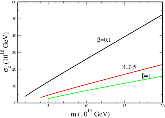
Figure 5.1: The critical value $\sigma_{c}$ of the inflaton field as a function of the mass parameter $m$ for $\kappa=\lambda=3\,\cdot 10^{-3}$ and $\beta=0.1$, $0.5$ and $1$, as indicated on the curves.

A better set of values [43] is $m=2\,\cdot 10^{15}\,\rm{GeV}$, $\kappa=\lambda=5\,\cdot 10^{-3}$ and $\beta=0.1$, which also yield $\sigma_{c}\simeq 4\,\cdot 10^{16}\,\rm{GeV}$. In this case, $\sigma_{f}\simeq 1.7\,\cdot 10^{17}\,\rm{GeV}$ and $\sigma_{Q}\simeq 1.6\,\cdot 10^{18}\,\rm{GeV}$, which are much smaller but still close to $m_{\rm P}$. Values of $\beta$ smaller than $0.1$ (with suitable values of the other parameters) give also very similar results. Actually, it turns out [43] that a general feature of the new shifted hybrid inflationary model is that the relevant part of inflation occurs at large values of $\sigma$, which are close to $m_{\rm P}$. Consequently, one is obliged to consider the SUGRA corrections to the scalar potential and invoke [43] some mechanism to ensure that the new shifted inflationary path remains flat. We will address this issue in the next section.

We will now shortly discuss the constraints imposed on the parameter space by the measurements on the power spectrum amplitude $P_{\mathcal{R}}^{1/2}$ of the primordial curvature perturbation. For a fixed $P_{\mathcal{R}}^{1/2}$ we can determine one of the free parameters (say $\beta$) in terms of the others ($m$, $\kappa$ and $\lambda$). For instance, the COBE [44] constraint $P_{\mathcal{R}}^{1/2}\simeq 5.11\,\cdot 10^{-5}$, corresponds to $\beta=0.1$ if $m=4.35\,\cdot 10^{15}\,\rm{GeV}$ and $\kappa=\lambda=3\,\cdot 10^{-2}$. In this case, $\sigma_{c}\simeq 3.55\,\cdot 10^{16}\,\rm{GeV}$, $\sigma_{f}\simeq 1.7\,\cdot 10^{17}\,\rm{GeV}$ and $\sigma_{Q}\simeq 1.6\,\cdot 10^{18}\,\rm{GeV}$. Also, $M\simeq 2.66\,\cdot 10^{16}\,\rm{GeV}$, $N_{Q}\simeq 57.7$ and $n_{\rm s}\simeq 0.98$. We see that the constraint on the power spectrum amplitude can be easily satisfied with natural values of the parameters. Moreover, superheavy SM non-singlets with masses $\ll M_{\rm GUT}$, which could disturb the unification of the SM gauge couplings, are not encountered.

5.4 Supergravity corrections

As we emphasized, new shifted hybrid inflation occurs at values of $\sigma$ which are quite close to the reduced Planck scale. Thus, one cannot ignore the SUGRA corrections to the scalar potential. The F-term scalar potential in SUGRA is given by Eq. (2.56), which is rewritten here for convenience

$$V=e^{K/m_{\rm P}^{2}}\left[(K^{-1})_{i}^{j}\;F^{i*}F_{j}-3|W|^{2}/m_{\rm P}^{2}\right],$$ (5.41)

with $F^{i*}=-(W^{i}+WK^{i}/m_{\rm P}^{2})$, $F_{j}=-(W_{j}^{*}+W^{*}K_{j}/m_{\rm P}^{2})$. $(K^{-1})_{i}^{j}$ is the inverse of the Kähler metric $K_{i}^{j}$ and a raised (lowered) index $i$ corresponds to derivation with respect to $\phi_{i}$ ($\phi^{i*}$).

Consider a (complex) inflaton $\Sigma$ corresponding to a flat direction of global SUSY with $W_{i\Sigma}=0$. We assume that the potential on this path depends only on $|\Sigma|$, which holds in this model due to a global symmetry. From Eq. (5.41), we find that the SUGRA corrections lift the flatness of the $\Sigma$ direction by generating a mass squared for $\Sigma$ (see e.g. [45])

$$m_{\Sigma}^{2}=\frac{V_{0}}{m_{\rm P}^{2}}-\frac{|W_{\Sigma}|^{2}}{m_{\rm P}^{2}}+\sum_{i,j}W^{i*}(K^{-1})_{i\Sigma\Sigma^{*}}^{j}W_{j}+\cdots,$$ (5.42)

where the right hand side (RHS) is evaluated on the flat direction with the explicitly displayed terms taken at $\Sigma=0$. The ellipsis represents higher order terms which are suppressed by powers of $|\Sigma|/m_{\rm P}$. The slow roll parameter $\eta$ then becomes

$$\eta=1-\frac{|W_{\Sigma}|^{2}}{V_{0}}+\frac{m_{\rm P}^{2}}{V_{0}}\sum_{i,j}W^{i*}(K^{-1})_{i\Sigma\Sigma^{*}}^{j}W_{j}+\cdots,$$ (5.43)

which, in general, could be of order unity and thus invalidate [14] inflation. This is the well known $\eta$ problem of inflation in local SUSY. Several proposals have been made in the literature to overcome this difficulty (for a review see e.g. [45]).

In standard and shifted hybrid inflation, there is an automatic mutual cancellation between the first two terms in the RHS of Eq. (5.43). This is due to the fact that $W_{n}=0$ on the inflationary path for all field directions $n$ which are perpendicular to this path, which implies that $|W_{\Sigma}|^{2}=V_{0}$ on the path. This is an important feature of these models since, in general, the sum of the first two terms in the RHS of Eq. (5.43) is positive and of order unity, thereby ruining inflation. It is easily checked that these properties persist in this inflationary model too. In particular, the superpotential on the new shifted inflationary path takes the form $W=V_{0}^{1/2}\Sigma$.

In all these hybrid inflation models, the only non-zero contribution from the sum which appears in the RHS of Eq. (5.43) originates from the term with $i=j=\Sigma$ (recall that $W_{n}=0$ on the path). This contribution is equal to the dimensionless coefficient of the quartic term $|\Sigma|^{4}/4m_{\rm P}^{2}$ in the Kähler potential. For inflation to remain intact, we need to assume that this coefficient is somewhat small. The remaining terms give negligible contributions to $\eta$ provided that $|\Sigma|\ll m_{\rm P}$. The latter is true for standard and shifted hybrid inflation. So, we see that, in these models, a mild tuning of just one parameter is adequate for protecting inflation from SUGRA corrections.

In the present model, however, inflation takes place at values of $|\Sigma|$ close to $m_{\rm P}$. So, the terms in the ellipsis in the RHS of Eq. (5.43) cannot be ignored and may easily invalidate inflation. Thus, one needs to invoke [43] here a mechanism which can ensure that the SUGRA corrections do not lift the flatness of the inflationary path to all orders. A suitable scheme has been suggested in [46]. It has been argued that special forms of the Kähler potential can lead to the cancellation of the SUGRA corrections which spoil slow roll inflation to all orders. In particular, a specific form of $K(\Sigma)$ (used in no-scale SUGRA models) was employed and a gauge singlet field $Z$ with a similar $K(Z)$ was introduced. It was pointed out that, by assuming a superheavy VEV for the $Z$ field through D-terms, an exact cancellation of the inflaton mass on the inflationary trajectory can be achieved.

The mechanism of Ref. [46] can be readily incorporated [43] in the new shifted hybrid inflation model we have been discussing, to ensure that the SUGRA corrections do not lift the flatness of the inflationary path. The only alteration caused to the lagrangian along this path is that the kinetic term of $\sigma$ is now non-minimal. This affects the equation of motion of $\sigma$ and, consequently, the slow roll conditions, $P_{\mathcal{R}}^{1/2}$ and $N_{Q}$. The form of the Kähler potential for $\Sigma$ used in [46] is

$$K(|\Sigma|^{2})=-Nm_{\rm P}^{2}\ln\left(1-\frac{|\Sigma|^{2}}{Nm_{\rm P}^{2}}\right),$$ (5.44)

where $N=1$ or $2$. Here we take $N=2$. In this case, the kinetic term of the real normalized inflaton field $\sigma$ (recall that $|\Sigma|=\sigma/\sqrt{2}$) is $(1/2)(\partial^{2}K/\partial\Sigma\partial\Sigma^{*})\dot{\sigma}^{2}$, where the overdot denotes derivation with respect to the cosmic time $t$ and $\partial^{2}K/\partial\Sigma\partial\Sigma^{*}=(1-\sigma^{2}/2Nm_{\rm P}^{2})^{-2}$. Thus, the lagrangian on the new shifted path is given by

$$L=\int_{-\infty}^{\infty}dt\int d^{3}x\,a^{3}(t)\left[\frac{1}{2}\,\dot{\sigma}^{2}\left(1-\frac{\sigma^{2}}{2Nm_{\rm P}^{2}}\right)^{-2}-V(\sigma)\right],$$ (5.45)

where $a(t)$ is the scale factor of the universe.

The evolution equation of $\sigma$ is found by varying this lagrangian with respect to $\sigma$

$$\left[\ddot{\sigma}+3H\dot{\sigma}+\dot{\sigma}^{2}\left(1-\frac{\sigma^{2}}{2Nm_{\rm P}^{2}}\right)^{-1}\frac{\sigma}{Nm_{\rm P}^{2}}\right]\left(1-\frac{\sigma^{2}}{2Nm_{\rm P}^{2}}\right)^{-2}+V^{\prime}(\sigma)=0,$$ (5.46)

where $H$ is the Hubble parameter. During inflation, the “friction” term $3H\dot{\sigma}$ dominates over the other two terms in the brackets in Eq. (5.46). Thus, this equation reduces to the “modified” inflationary equation

$$\dot{\sigma}=-\frac{V^{\prime}(\sigma)}{3H}\left(1-\frac{\sigma^{2}}{2Nm_{\rm P}^{2}}\right)^{2}.$$ (5.47)

Note that, for $\sigma\ll\sqrt{2N}m_{\rm P}$, this equation reduces to the standard inflationary equation.

To derive the slow roll conditions, we evaluate the sum of the first and the third term in the brackets in Eq. (5.46) by using Eq. (5.47):

$$\ddot{\sigma}+\dot{\sigma}^{2}\left(1-\frac{\sigma^{2}}{2Nm_{\rm P}^{2}}\right)^{-1}\frac{\sigma}{Nm_{\rm P}^{2}}=\frac{V^{\prime}(\sigma)}{3H^{2}}H^{\prime}(\sigma)\dot{\sigma}\left(1-\frac{\sigma^{2}}{2Nm_{\rm P}^{2}}\right)^{2}$$

$$\hskip 28.45274pt-\frac{V^{\prime\prime}(\sigma)}{3H}\dot{\sigma}\left(1-\frac{\sigma^{2}}{2Nm_{\rm P}^{2}}\right)^{2}+\frac{V^{\prime}(\sigma)}{3H}\dot{\sigma}\left(1-\frac{\sigma^{2}}{2Nm_{\rm P}^{2}}\right)\frac{\sigma}{Nm_{\rm P}^{2}}\cdot$$ (5.48)

Comparing the first two terms in the RHS of Eq. (5.48) with $H\dot{\sigma}$, we obtain

$$\epsilon\simeq\frac{m_{\rm P}^{2}}{2}\left(\frac{V^{\prime}(\sigma)}{V_{0}}\right)^{2}\left(1-\frac{\sigma^{2}}{2Nm_{\rm P}^{2}}\right)^{2}\leq 1,\quad|\eta|\simeq m_{\rm P}^{2}\left|\frac{V^{\prime\prime}(\sigma)}{V_{0}}\right|\left(1-\frac{\sigma^{2}}{2Nm_{\rm P}^{2}}\right)^{2}\leq 1.$$ (5.49)

The third term in the RHS of Eq. (5.48), compared to $H\dot{\sigma}$, yields $\sqrt{2}\sigma\epsilon^{1/2}/Nm_{\rm P}\leq 1$, which is automatically satisfied provided that $\epsilon\leq 1$ and $\sigma\leq Nm_{\rm P}/\sqrt{2}$. The latter is true for the values of $\sigma$ which are relevant here. We see that the slow roll parameters $\epsilon$ and $\eta$ now carry an extra factor $(1-\sigma^{2}/2Nm_{\rm P}^{2})^{2}\leq 1$. This leads, in general, to smaller $\sigma_{f}$’s. However, in the present case $\sigma_{f}\ll\sqrt{2N}m_{\rm P}$ (for $N=2$) and, thus, this factor is practically equal to unity. Consequently, its influence on $\sigma_{f}$ is negligible.

The formulas for $N_{Q}$ and $P_{\mathcal{R}}^{1/2}$ are now also modified due to the presence of the extra factor $(1-\sigma^{2}/2Nm_{\rm P}^{2})^{2}$ in Eq. (5.47). In particular, a factor $(1-\sigma^{2}/2Nm_{\rm P}^{2})^{-2}$ must be included in the integrand in the RHS of Eq. (3.13) and a factor $(1-\sigma_{Q}^{2}/2Nm_{\rm P}^{2})^{-4}$ in the RHS of Eq. (3.14). One finds [43] that, for the $\sigma$’s under consideration, these modifications have only a small influence on $\sigma_{Q}$ if one uses the same input values for the free parameters as in the global SUSY case. On the contrary, $P_{\mathcal{R}}^{1/2}$ increases considerably. However, we can easily readjust the parameters so that the observational requirements on the power spectrum are again met. For instance, $P_{\mathcal{R}}^{1/2}\simeq 5.11\,\cdot 10^{-5}$ is now obtained with $m=3.8\,\cdot 10^{15}\,\rm{GeV}$, keeping $\kappa=\lambda=3\,\cdot 10^{-2}$ and $\beta=0.1$ as in global SUSY. In this case, $\sigma_{c}\simeq 2.7\,\cdot 10^{16}\,\rm{GeV}$, $\sigma_{f}\simeq 1.8\,\cdot 10^{17}\,\rm{GeV}$ and $\sigma_{Q}\simeq 1.6\,\cdot 10^{18}\,\rm{GeV}$. Also, $M\simeq 2.6\,\cdot 10^{16}\,\rm{GeV}$, $N_{Q}\simeq 57.5$ and $n\simeq 0.99$.

Chapter 6 Semi-shifted hybrid inflation with $\rm B-L$ cosmic strings

6.1 Introduction

As we have seen, one of the most promising models for inflation is, undoubtedly, hybrid inflation, which is naturally realized within SUSY GUT models. In the standard realization of SUSY hybrid inflation, the spontaneous breaking of the GUT gauge symmetry takes place at the end of inflation and, thus, superheavy magnetic monopoles [47] are copiously produced if they are predicted by this symmetry breaking. In this case, a cosmological catastrophe is encountered. In order to avoid this disaster, one can employ the smooth or shifted variants of SUSY hybrid inflation (see Chap. 3). In these inflationary scenarios, which, in their original realization, are based on non-renormalizable superpotential terms, the GUT gauge symmetry is broken to the SM gauge group already during inflation and, thus, no magnetic monopoles are produced at the termination of inflation. A new version of the shifted inflationary scheme can be implemented, as we saw in Chap. 5, with only renormalizable superpotential terms, within the extended SUSY PS model introduced in Chap. 4.

Fitting the three-year data of the Wilkinson microwave anisotropy probe (WMAP) satellite with the standard power-law cosmological model with cold dark matter and a cosmological constant ($\Lambda$CDM), one obtains [11] values of the spectral index $n_{\rm s}$ which are clearly lower than unity. However, in supergravity with canonical Kähler potential, the above hybrid inflation models yield [20] $n_{\rm s}$’s which are very close to unity or even larger than it, although their running is negligible. This discrepancy may be resolved [15, 21, 48] by including non-minimal terms in the Kähler potential. Alternatively, if we wish to stick to minimal SUGRA, we can reduce [49] the spectral index predicted by the hybrid inflationary models by restricting the number of e-foldings suffered by our present horizon scale during the hybrid inflation which generates the observed curvature perturbations. The additional number of e-foldings required for solving the horizon and flatness problems of standard hot big bang cosmology can be provided by a subsequent second stage of inflation. In Chap. 8, we will show that the same extended SUSY PS model can lead to a two-stage inflationary scenario yielding acceptable $n_{\rm s}$’s in minimal SUGRA. The first stage of inflation, during which the cosmological scales exit the horizon, is of the standard hybrid type, while the second stage, which provides the additional e-foldings, is of the smooth hybrid type.

In this chapter, we consider an alternative inflationary scenario [50] which incorporates cosmic strings [51] (for a textbook presentation or a review, see e.g. [52]) and can also be naturally realized within the same extended SUSY PS model with only renormalizable superpotential terms. As shown in Chap. 5, this model possesses a shifted classically flat direction along which $\rm U(1)_{B-L}$ is unbroken. In order to distinguish it from the new shifted flat direction on which $G_{\rm PS}$ is broken to $G_{\rm SM}$, we call this flat direction “semi-shifted”. This direction acquires, as usual, a logarithmic slope from one-loop radiative corrections which are due to the SUSY breaking caused by the non-zero potential energy density on it. So, it can perfectly well be used as an inflationary path along which semi-shifted hybrid inflation takes place. When the system crosses the critical point at which this path is destabilized, a waterfall regime occurs during which the $\rm U(1)_{B-L}$ gauge symmetry breaks spontaneously and local cosmic strings are produced. The resulting string network can then contribute to the primordial curvature perturbations.

It has been argued [53] that in the presence of a small contribution to the curvature perturbation from cosmic strings, the current cosmic microwave background data can allow values of the spectral index that are larger than the ones obtained in the absence of strings. Therefore, we may hope that the semi-shifted hybrid inflationary scenario, which does involve cosmic strings, can be made compatible with the CMBR data, even without the use of non-minimal terms in the Kähler potential or a subsequent complementary stage of inflation. Recently, a fit to the CMBR data and the luminous red galaxy data in the Sloan digital sky survey (SDSS) [54] on large length scales outside the non-linear regime was performed [55] by using field-theory simulations [56] of a dynamical network of local cosmic strings. It demonstrated that the Harrison-Zeldovich (HZ) model (i.e. with $n_{\rm s}=1$) with a fractional contribution $f_{10}\simeq 0.10$ from cosmic strings to the temperature power spectrum at multipole $\ell=10$, is even moderately favored over the standard power-law model without strings. For the power-law $\Lambda$CDM cosmological model with cosmic strings this fit yields $n_{\rm s}=0.94-1.06$ and $f_{10}=0.02-0.18$ at $95\%$ confidence level (c.l.). As we will see, under these circumstances the semi-shifted hybrid inflation model in minimal SUGRA can easily be compatible with the data. Note that there is obviously no formation of PS magnetic monopoles at the end of the semi-shifted hybrid inflation and, thus, the corresponding cosmological catastrophe is avoided.

6.2 Semi-shifted hybrid inflation in global SUSY

We consider the extended SUSY PS model described in Chap. 4, which can lead to a moderate violation of the asymptotic Yukawa unification so that, for $\mu>0$, an acceptable $b$-quark mass is obtained even with universal boundary conditions. The breaking of $G_{\rm PS}$ to $G_{\rm SM}$ is achieved by the superheavy VEVs of the right handed neutrino type components of a conjugate pair of Higgs superfields $H^{c}$ and $\bar{H}^{c}$ belonging to the $({\bf\bar{4},1,2})$ and $({\bf 4,1,2})$ representations of $G_{\rm PS}$ respectively. The model also contains a gauge singlet $S$ and a conjugate pair of superfields $\phi$, $\bar{\phi}$ belonging to the $({\bf 15,1,3})$ representation of $G_{\rm PS}$. The superfield $\phi$ acquires a VEV which breaks $G_{\rm PS}$ to $G_{\rm SM}\times{\rm U(1)_{B-L}}$. In addition to $G_{\rm PS}$, the model possesses a $Z_{2}$ matter parity symmetry and two global $\rm U(1)$ symmetries, namely a Peccei-Quinn and a R symmetry. Such continuous global symmetries can effectively arise [57] from the rich discrete symmetry groups encountered in many compactified string theories (see e.g. [58]). As we have seen in Chap. 5, this model can lead to new shifted hybrid inflation based solely on renormalizable interactions.

The superpotential terms which are relevant for inflation are given in Eq. (5.1). These terms, with a different (more convenient for our purposes here) choice of basic parameters and their phases, can be rewritten as

$$W=\kappa S(M^{2}-\phi^{2})-\gamma SH^{c}\bar{H}^{c}+m\phi\bar{\phi}-\lambda\bar{\phi}H^{c}\bar{H}^{c},$$ (6.1)

where $M$, $m$ are superheavy masses of the order of the SUSY GUT scale $M_{\rm GUT}\simeq 2.86\,\cdot 10^{16}\,\rm{GeV}$ and $\kappa$, $\gamma$, $\lambda$ are dimensionless coupling constants. These parameters are normalized so that they correspond to the couplings between the SM singlet components of the superfields. In a general superpotential of the type in Eq. (6.1), $M$, $m$ and any two of the three dimensionless parameters $\kappa$, $\gamma$, $\lambda$ can always be made real and positive by appropriately redefining the phases of the superfields. The third dimensionless parameter, however, remains generally complex. For definiteness, we will choose here this parameter to be real and positive too. One can show that the superpotential in Eq. (5.1) with the particular choice of the phases of its parameters considered there, can become equivalent to the superpotential in Eq. (6.1) provided that two of its real and positive parameters are rotated to the negative real axis. Actually, the form of the superpotential in Eq. (6.1) can be derived from the one in Eq. (5.1) by the replacement: $\kappa\to-\gamma$, $\lambda\to-\lambda$, $\beta\to\kappa$, $M^{2}\to(\kappa/\gamma)M^{2}$. The F-term scalar potential obtained from the superpotential $W$ in Eq. (6.1) is given by

$$V=|\kappa\,(M^{2}-\phi^{2})-\gamma H^{c}\bar{H}^{c}|^{2}+|m\bar{\phi}-2\kappa S\phi|^{2}+|m\phi-\lambda H^{c}\bar{H}^{c}|^{2}+|\gamma S+\lambda\bar{\phi}\,|^{2}\left(|H^{c}|^{2}+|\bar{H}^{c}|^{2}\right),$$ (6.2)

where the complex scalar fields which belong to the SM singlet components of the superfields are denoted by the same symbol. We will ignore throughout the soft SUSY breaking terms [59] in the scalar potential since their effect on inflationary dynamics is negligible in our case as in the case of the conventional realization of shifted hybrid inflation.

From Eq. (6.2) and the vanishing of the D-terms (which implies that $\bar{H}^{c*}=e^{i\theta}H^{c}$), we find [60] that there exist two distinct continua of SUSY vacua:

$$\phi=\phi_{+},\quad\bar{H}^{c*}=H^{c},\quad|H^{c}|=\sqrt{\frac{m\phi_{+}}{\lambda}}\quad(\theta=0),$$ (6.3)

$$\phi=\phi_{-},\quad\bar{H}^{c*}=-H^{c},\quad|H^{c}|=\sqrt{\frac{-m\phi_{-}}{\lambda}}\quad(\theta=\pi),$$ (6.4)

with $\bar{\phi}=S=0$, where

$$\phi_{\pm}\equiv\frac{\gamma m}{2\kappa\lambda}\left(-1\pm\sqrt{1+\frac{4\kappa^{2}\lambda^{2}M^{2}}{\gamma^{2}m^{2}}}\,\right).$$ (6.5)

It has been shown in Chap. 5 (see also [60]) that the potential in Eq. (6.2) generally possesses three flat directions. The first one is the usual trivial flat direction at $\phi=\bar{\phi}=H^{c}=\bar{H}^{c}=0$ with $V=V_{\rm tr}\equiv\kappa^{2}M^{4}$. The second one, which appears at

$$\phi=-\frac{\gamma m}{2\kappa\lambda},\quad\bar{\phi}=-\frac{\gamma}{\lambda}\,S,\quad H^{c}\bar{H}^{c}=\frac{\kappa\gamma(M^{2}-\phi^{2})+\lambda m\phi}{\gamma^{2}+\lambda^{2}},$$ (6.6)

$$V=V_{\rm nsh}\equiv\frac{\kappa^{2}\lambda^{2}}{\gamma^{2}+\lambda^{2}}\left(M^{2}+\frac{\gamma^{2}m^{2}}{4\kappa^{2}\lambda^{2}}\right)^{2},$$ (6.7)

exists only for $\gamma\neq 0$ and is the trajectory for the new shifted hybrid inflation. Along this direction, $G_{\rm PS}$ is broken to $G_{\rm SM}$. The third flat direction exists only if $\tilde{M}^{2}\equiv M^{2}-m^{2}/2\kappa^{2}>0$ and lies at

$$\phi=\pm\,\tilde{M},\quad\bar{\phi}=\frac{2\kappa\phi}{m}\,S,\quad H^{c}=\bar{H}^{c}=0.$$ (6.8)

It is a “semi-shifted” flat direction (in the sense that, although the field $\phi$ is shifted from zero, the fields $H^{c}$, $\bar{H}^{c}$ remain zero on it) with

$$V=V_{\rm ssh}\equiv\kappa^{2}(M^{4}-\tilde{M}^{4}).$$ (6.9)

Along this direction $G_{\rm PS}$ is broken to $G_{\rm SM}\times{\rm U(1)_{B-L}}$.

In our subsequent discussion, we will concentrate on the case where $\tilde{M}^{2}>0$. It is interesting to note that, in this case, the trivial flat direction is unstable [60] as it is a path of saddle points of the potential. Moreover, for $\tilde{M}^{2}>0$, we always have $V_{\rm ssh}<V_{\rm nsh}$. It is, thus, more likely that the system will eventually settle down on the semi-shifted rather than the new shifted flat direction. Semi-shifted hybrid inflation can then take place as the system slowly rolls down the semi-shifted path driven by its logarithmic slope provided by one-loop radiative corrections, which are due to the SUSY breaking by the non-vanishing potential energy density on this path. As the system crosses the critical point of the semi-shifted path, the $\rm U(1)_{B-L}$ gauge symmetry breaks, generating a network of local cosmic strings, which contribute a small amount to the CMBR temperature power spectrum. As mentioned, for models with local cosmic strings, it has been shown in [55] that, at $95\%$ c.l., $n_{\rm s}=0.94-1.06$ and $f_{10}=0.02-0.18$.

6.3 One-loop radiative corrections

The one-loop radiative correction to the potential on the semi-shifted path is calculated by the Coleman-Weinberg formula:

$$\Delta V=\frac{1}{64\pi^{2}}\,\sum_{i}(-1)^{F_{i}}M_{i}^{4}\ln\frac{M_{i}^{2}}{\Lambda^{2}},$$ (6.10)

where the sum extends over all helicity states $i$, $F_{i}$ and $M_{i}^{2}$ are the fermion number and mass squared of the $i$th state and $\Lambda$ is a renormalization mass scale. In order to use this formula for creating a logarithmic slope in the inflationary potential, one has first to derive the mass spectrum of the model on the semi-shifted path.

As mentioned, during semi-shifted hybrid inflation, the SM singlet components of $\phi$, $\bar{\phi}$ acquire non-vanishing values and break $G_{\rm PS}$ to $G_{\rm SM}\times{\rm U(1)_{B-L}}$. The value of the complex scalar field $S$ at a point of the semi-shifted path is taken real by an appropriate R transformation. For simplicity, we use the same symbol $S$ for this real value of the field as for the complex field in general since the distinction will be obvious from the context. The deviation of the complex scalar field $S$ from its (real) value at a point of the inflationary path is denoted by $\delta S$. We can further write $\phi=v+\delta\phi$, $\bar{\phi}=\bar{v}+\delta\bar{\phi}$ with $v=\pm\tilde{M}$, $\bar{v}=(2\kappa v/m)\,S$ and $\delta\phi$, $\delta\bar{\phi}$ being complex scalar fields. We can then define the canonically normalized complex scalar fields

$$\zeta=\frac{2\kappa v\,\delta S-m\delta\bar{\phi}}{(m^{2}+4\kappa^{2}v^{2})^{1/2}},\quad\epsilon=\frac{m\delta S+2\kappa v\,\delta\bar{\phi}}{(m^{2}+4\kappa^{2}v^{2})^{1/2}}.$$ (6.11)

We find that $\epsilon$ remains massless on the semi-shifted path. So, it corresponds to the complex scalar inflaton field $\Sigma=(mS+2\kappa v\bar{\phi})/(m^{2}+4\kappa^{2}v^{2})^{1/2}$, which during inflation takes the form $\Sigma=(1+4\kappa^{2}v^{2}/m^{2})^{1/2}S$. Consequently, in our case, the real canonically normalized inflaton is

$$\sigma=2^{1/2}(1+4\kappa^{2}v^{2}/m^{2})^{1/2}S,$$ (6.12)

where $S$ is obviously rotated to be real.

Expanding the complex scalars $\zeta$, $\delta\phi$, $H^{c}$ and $\bar{H}^{c}$ in real and imaginary parts according to the prescription $\chi=(\chi_{1}+i\chi_{2})/\sqrt{2}$, we find that the mass-squared matrices $M_{-}^{2}$ of $\zeta_{1}$, $\delta\phi_{1}$, $M_{+}^{2}$ of $\zeta_{2}$, $\delta\phi_{2}$, $M_{1}^{2}$ of $H^{c}_{1}$, $\bar{H}^{c}_{1}$ and $M_{2}^{2}$ of $H^{c}_{2}$, $\bar{H}^{c}_{2}$ are given by

$$M_{\pm}^{2}=m^{2}\left(\begin{array}[]{cc}1+a^{2}&s(1+a^{2})^{1/2}\\ s(1+a^{2})^{1/2}&1+a^{2}+s^{2}\pm 1\end{array}\right),$$ (6.15)

$$M_{1,2}^{2}=m^{2}\left(\begin{array}[]{cc}s^{2}b^{2}&\mp b\\ \mp b&s^{2}b^{2}\end{array}\right),$$ (6.18)

where $a=2\kappa v/m$, $b=(\gamma+\lambda a)/2\kappa$ and $s=2\kappa S/m$. Note that the eigenvalues of the matrices $M_{\pm}^{2}$ are always positive. Though, this is not the case with $M_{1,2}^{2}$. Specifically, one of the two eigenvalues of each of these matrices is always positive while the other one becomes negative for $|s|<s_{c}\equiv 1/\sqrt{|b|}$ (we assume that $b\neq 0$). This defines the critical point on the semi-shifted path at which this path is destabilized (see below).

The superpotential in Eq. (6.1) gives rise to mass terms between the fermionic partners of $\zeta$, $\delta\phi$ and $H^{c}$, $\bar{H}^{c}$ (the fermionic partner of $\epsilon$ remains massless). The squares of the corresponding mass matrices are found to be

$$M_{0}^{2}=m^{2}\left(\begin{array}[]{cc}1+a^{2}&s(1+a^{2})^{1/2}\\ s(1+a^{2})^{1/2}&1+a^{2}+s^{2}\end{array}\right),$$ (6.21)

$$\bar{M}_{0}^{2}=m^{2}\left(\begin{array}[]{cc}s^{2}b^{2}&0\\ 0&s^{2}b^{2}\end{array}\right).$$ (6.24)

This completes the analysis of the SM singlet sector of the model. In summary, we found four groups of two real scalars with mass-squared matrices $M_{+}^{2}$, $M_{-}^{2}$, $M_{1}^{2}$ and $M_{2}^{2}$ and two groups of two Weyl fermions with mass matrices squared $M_{0}^{2}$ and $\bar{M}_{0}^{2}$. The contribution of the SM singlet sector to the radiative corrections to the potential along the semi-shifted path is given by

$$\Delta V=\frac{1}{64\pi^{2}}\,\operatorname{Tr}\Bigg{\{}M_{+}^{4}\ln\frac{M_{+}^{2}}{\Lambda^{2}}+M_{-}^{4}\ln\frac{M_{-}^{2}}{\Lambda^{2}}-2M_{0}^{4}\ln\frac{M_{0}^{2}}{\Lambda^{2}}+M_{1}^{4}\ln\frac{M_{1}^{2}}{\Lambda^{2}}+M_{2}^{4}\ln\frac{M_{2}^{2}}{\Lambda^{2}}-2\bar{M}_{0}^{4}\ln\frac{\bar{M}_{0}^{2}}{\Lambda^{2}}\Bigg{\}}.$$ (6.25)

We now turn to the $u^{c}$, $\bar{u}^{c}$ type fields which are color antitriplets with charge $-2/3$ and color triplets with charge $2/3$ respectively. Such fields exist in $H^{c}$, $\bar{H}^{c}$, $\phi$ and $\bar{\phi}$ and we shall denote them by $u_{H}^{c}$, $\bar{u}_{H}^{c}$, $u_{\phi}^{c}$, $\bar{u}_{\phi}^{c}$, $u_{\bar{\phi}}^{c}$ and $\bar{u}_{\bar{\phi}}^{c}$. The relevant expansion of $\phi$ is given in Eq. (5.22).

In the bosonic $u^{c}$, $\bar{u}^{c}$ type sector, we find that the mass-squared matrices $M_{u\pm}^{2}$ of the complex scalar fields $u_{\chi\pm}^{c}=(u_{\chi}^{c}\pm\bar{u}_{\chi}^{c*})/\sqrt{2}$, for $\chi=H,\phi,\bar{\phi}$, are

$$M_{u+}^{2}=m^{2}\left(\begin{array}[]{ccc}c^{2}s^{2}-c&0&0\\ 0&s^{2}&-s\\ 0&-s&1\end{array}\right),$$ (6.29)

$$M_{u-}^{2}=m^{2}\left(\begin{array}[]{ccc}c^{2}s^{2}+c&0&0\\[3.0pt] 0&2+s^{2}+\rho_{g}^{2}&-s(1-\rho_{g}^{2})\\[3.0pt] 0&-s(1-\rho_{g}^{2})&1+\rho_{g}^{2}s^{2}\end{array}\right),$$ (6.33)

where $c=(\gamma-\lambda a/3)/2\kappa$ and $\rho_{g}^{2}=g^{2}a^{2}/3\kappa^{2}$ with $g$ being the $G_{\rm PS}$ gauge coupling constant. Note that $\rho_{g}^{2}$ parameterizes contributions arising from the D-terms of the scalar potential and $M_{u+}^{2}$ has one zero eigenvalue corresponding to the Goldstone boson which is absorbed by the superhiggs mechanism. Furthermore, one of the eigenvalues $m^{2}(c^{2}s^{2}\mp c)$ of the matrices in Eqs. (6.29) and (6.33) (depending on the sign of $c$) becomes negative as soon as $s$ crosses below the point $s_{c}^{(1)}\equiv 1/\sqrt{|c|}$ on the semi-shifted path. So, if $s_{c}^{(1)}$ was larger than the critical value $s_{c}$, the system would be destabilized first in one of the directions $u_{H\pm}^{c}$. In this case, a $\rm SU(3)_{c}$-breaking VEV would develop. To avoid this, we should demand that $s_{c}^{(1)}$ is located lower than the critical point $s_{c}$, so that, after the end of inflation, the correct symmetry breaking is obtained. This gives the condition $|b|<|c|$, which we will consider later.

In the fermionic $u^{c}$, $\bar{u}^{c}$ type sector, we obtain four Dirac fermions (per color): $\psi_{u_{H}^{c}}^{D}=\psi_{u_{H}^{c}}+\psi^{c}_{\bar{u}_{H}^{c}}$, $\psi_{u_{\phi}^{c}}^{D}=\psi_{u_{\phi}^{c}}+\psi^{c}_{\bar{u}_{\phi}^{c}}$, $\psi_{u_{\bar{\phi}}^{c}}^{D}=\psi_{u_{\bar{\phi}}^{c}}+\psi^{c}_{\bar{u}_{\bar{\phi}}^{c}}$ and $-i\lambda^{D}=-i(\lambda^{+}+\lambda^{-c})$. Here, $\psi_{\chi}$ is the fermionic partner of the complex scalar field $\chi$ and $\lambda^{\pm}=(\lambda^{1}\pm i\lambda^{2})/\sqrt{2}$, where $\lambda^{1}$ ($\lambda^{2}$) is the gaugino color triplet corresponding to the ${\rm SU}(4)_{c}$ generators with $1/2$ ($-i/2$) in the $i4$ and $1/2$ ($i/2$) in the $4i$ entry ($i=1,2,3$). The fermionic mass matrix is

$$M_{\psi_{u}}=m\left(\begin{array}[]{cccc}-cs&0&0&0\\ 0&-s&1&-\rho_{g}\\ 0&1&0&-\rho_{g}s\\ 0&-\rho_{g}&-\rho_{g}s&0\end{array}\right).$$ (6.34)

To complete this sector, we must also include the gauge bosons $A^{1,2}$ which are associated with $\lambda^{1,2}$. They acquire a mass squared $M_{g}^{2}=m^{2}\rho_{g}^{2}(1+s^{2})$.

The overall contribution of the $u^{c}$, $\bar{u}^{c}$ type sector to $\Delta V$ in Eq. (6.10) is

$$\Delta V=\frac{3}{32\pi^{2}}\operatorname{Tr}\Bigg{\{}M_{u+}^{4}\ln\frac{M_{u+}^{2}}{\Lambda^{2}}+M_{u-}^{4}\ln\frac{M_{u-}^{2}}{\Lambda^{2}}-2M_{\psi_{u}}^{4}\ln\frac{M_{\psi_{u}}^{2}}{\Lambda^{2}}+3M_{g}^{4}\ln\frac{M_{g}^{2}}{\Lambda^{2}}\Bigg{\}}.$$ (6.35)

We will now discuss the contribution from the $e^{c}$, $\bar{e}^{c}$ type sector consisting of color singlets with charge $1$, $-1$. Such fields exist in $H^{c}$, $\bar{H}^{c}$, $\phi$ and $\bar{\phi}$ and we shall denote them by $e_{H}^{c}$, $\bar{e}_{H}^{c}$, $e_{\phi}^{c}$, $\bar{e}_{\phi}^{c}$, $e_{\bar{\phi}}^{c}$ and $\bar{e}_{\bar{\phi}}^{c}$. The relevant expansion of $\phi$ is given in Eq. (5.27). It turns out that the mass terms in this sector are exactly the same as in the $u^{c}$, $\bar{u}^{c}$ type sector with $\lambda/3$ replaced by $\lambda$ and $2g^{2}/3$ by $g^{2}$. So, we will only summarize the results.

In the bosonic $e^{c}$, $\bar{e}^{c}$ type sector, the mass-squared matrices $M_{e\pm}^{2}$ of the complex scalars $e_{\chi\pm}^{c}=(e_{\chi}^{c}\pm\bar{e}_{\chi}^{c*})/\sqrt{2}$, for $\chi=H,\phi,\bar{\phi}$, are

$$M_{e+}^{2}=m^{2}\left(\begin{array}[]{ccc}d^{2}s^{2}-d&0&0\\ 0&s^{2}&-s\\ 0&-s&1\end{array}\right),$$ (6.39)

$$M_{e-}^{2}=m^{2}\left(\begin{array}[]{ccc}d^{2}s^{2}+d&0&0\\[3.0pt] 0&2+s^{2}+\tau_{g}^{2}&-s(1-\tau_{g}^{2})\\[3.0pt] 0&-s(1-\tau_{g}^{2})&1+\tau_{g}^{2}s^{2}\end{array}\right),$$ (6.43)

where $d=(\gamma-\lambda a)/2\kappa$ and $\tau_{g}=\sqrt{3/2}\,\rho_{g}$. Note that, again, $M_{e+}^{2}$ has one zero eigenvalue corresponding to the Goldstone boson which is absorbed by the superhiggs mechanism. Furthermore, one of the eigenvalues $m^{2}(d^{2}s^{2}\mp d)$ of the matrices in Eqs. (6.39) and (6.43) (depending on the sign of $d$) becomes negative as $s$ crosses below $s_{c}^{(2)}\equiv 1/\sqrt{|d|}$ on the semi-shifted path. Therefore, we must impose the constraint $s_{c}^{(2)}<s_{c}\Rightarrow|b|<|d|$ for the same reason explained above.

In the fermionic $e^{c}$, $\bar{e}^{c}$ type sector, we obtain four Dirac fermions with mass matrix

$$M_{\psi_{e}}=m\left(\begin{array}[]{cccc}-ds&0&0&0\\ 0&-s&1&-\tau_{g}\\ 0&1&0&-\tau_{g}s\\ 0&-\tau_{g}&-\tau_{g}s&0\end{array}\right).$$ (6.44)

Finally, we again obtain two gauge bosons with mass squared $\hat{M}_{g}^{2}=m^{2}\tau_{g}^{2}(1+s^{2})$.

The overall contribution of the $e^{c}$, $\bar{e}^{c}$ type sector to $\Delta V$ in Eq. (6.10) is

$$\Delta V=\frac{1}{32\pi^{2}}\operatorname{Tr}\Bigg{\{}M_{e+}^{4}\ln\frac{M_{e+}^{2}}{\Lambda^{2}}+M_{e-}^{4}\ln\frac{M_{e-}^{2}}{\Lambda^{2}}-2M_{\psi_{e}}^{4}\ln\frac{M_{\psi_{e}}^{2}}{\Lambda^{2}}+3\hat{M}_{g}^{4}\ln\frac{\hat{M}_{g}^{2}}{\Lambda^{2}}\Bigg{\}}.$$ (6.45)

Let us now consider the $d^{c}$, $\bar{d}^{c}$ type sector consisting of color antitriplets with charge $1/3$ and color triplets with charge $-1/3$. Such fields exist in $H^{c}$, $\bar{H}^{c}$, $\phi$ and $\bar{\phi}$ and we denote them by $d_{H}^{c}$, $\bar{d}_{H}^{c}$, $d_{\phi}^{c}$, $\bar{d}_{\phi}^{c}$, $d_{\bar{\phi}}^{c}$ and $\bar{d}_{\bar{\phi}}^{c}$. The field $\phi$ can be expanded in terms of these fields as in Eq. (5.32).

In the bosonic $d^{c}$, $\bar{d}^{c}$ type sector, the mass-squared matrices $M_{d\pm}^{2}$ of the complex scalars $d_{\chi\pm}^{c}=(d_{\chi}^{c}\pm\bar{d}_{\chi}^{c*})/\sqrt{2}$, for $\chi=H,\phi,\bar{\phi}$, are

$$M_{d\pm}^{2}=m^{2}\left(\begin{array}[]{ccc}e^{2}s^{2}\mp e&0&0\\ 0&1+s^{2}\mp 1&-s\\ 0&-s&1\end{array}\right),$$ (6.46)

where $e=(\gamma+\lambda a/3)/2\kappa$. Note that, again, one of the eigenvalues $m^{2}(e^{2}s^{2}\mp e)$ of these matrices (depending on the sign of $e$) becomes negative as $s$ crosses below $s_{c}^{(3)}\equiv 1/\sqrt{|e|}$ on the semi-shifted path and we, thus, have to impose the constraint $s_{c}^{(3)}<s_{c}\Rightarrow|b|<|e|$, so that the correct symmetry breaking pattern occurs at the end of inflation.

In the fermionic $d^{c}$, $\bar{d}^{c}$ type sector, we obtain three Dirac fermions (per color) with mass matrix

$$M_{\psi_{d}}=m\left(\begin{array}[]{ccc}-es&0&0\\ 0&-s&1\\ 0&1&0\end{array}\right).$$ (6.47)

Note that there are no D-terms, gauge bosons, or gauginos in this sector.

The contribution of this sector to $\Delta V$ in Eq. (6.10) is

$$\Delta V=\frac{3}{32\pi^{2}}\operatorname{Tr}\Bigg{\{}M_{d+}^{4}\ln\frac{M_{d+}^{2}}{\Lambda^{2}}+M_{d-}^{4}\ln\frac{M_{d-}^{2}}{\Lambda^{2}}-2M_{\psi_{d}}^{4}\ln\frac{M_{\psi_{d}}^{2}}{\Lambda^{2}}\Bigg{\}}.$$ (6.48)

Next, we consider the $q^{c}$, $\bar{q}^{c}$ type fields which are color antitriplets with charge $-5/3$ and color triplets with charge $5/3$. They exist in $\phi$, $\bar{\phi}$ and we call them $q_{\phi}^{c}$, $\bar{q}_{\phi}^{c}$, $q_{\bar{\phi}}^{c}$, $\bar{q}_{\bar{\phi}}^{c}$. The relevant expansion of $\phi$ can be found in Eq. (5.36).

In the bosonic $q^{c}$, $\bar{q}^{c}$ type sector, the mass-squared matrices $M_{q\pm}^{2}$ of the complex scalars $q_{\chi\pm}^{c}=(q_{\chi}^{c}\pm\bar{q}_{\chi}^{c*})/\sqrt{2}$, for $\chi=\phi,\bar{\phi}$, are

$$M_{q\pm}^{2}=m^{2}\left(\begin{array}[]{cc}1+s^{2}\mp 1&-s\\ -s&1\end{array}\right).$$ (6.49)

In the fermionic $q^{c}$, $\bar{q}^{c}$ type sector, we obtain two Dirac fermions (per color) with mass matrix

$$M_{\psi_{q}}=m\left(\begin{array}[]{cc}-s&1\\ 1&0\end{array}\right).$$ (6.50)

There are no D-terms, gauge bosons, or gauginos in this sector as well.

The contribution of this sector to $\Delta V$ in Eq. (6.10) is

$$\Delta V=\frac{3}{32\pi^{2}}\operatorname{Tr}\Bigg{\{}M_{q+}^{4}\ln\frac{M_{q+}^{2}}{\Lambda^{2}}+M_{q-}^{4}\ln\frac{M_{q-}^{2}}{\Lambda^{2}}-2M_{\psi_{q}}^{4}\ln\frac{M_{\psi_{q}}^{2}}{\Lambda^{2}}\Bigg{\}}.$$ (6.51)

Finally, in $\phi$, $\bar{\phi}$ there exist color octet, $\rm SU(2)_{R}$ triplet superfields: $\phi_{8}^{0}$, $\phi_{8}^{\pm}$, $\bar{\phi}_{8}^{0}$, $\bar{\phi}_{8}^{\pm}$, with charge $0$, $1$, $-1$ as indicated. The relevant expansion of $\phi$ is given in Eq. (5.39).

In the bosonic sector, we obtain two groups of 24 complex scalars, which can be combined in pairs of two with mass-squared matrix

$$M_{\phi_{8}\pm}^{2}=m^{2}\left(\begin{array}[]{cc}1+s^{2}\mp 1&-s\\ -s&1\end{array}\right).$$ (6.52)

In the fermionic sector, we find 48 Weyl fermions which can be combined in pairs of two with mass matrix

$$M_{\psi_{\phi_{8}}}=m\left(\begin{array}[]{cc}-s&1\\ 1&0\end{array}\right).$$ (6.53)

The contribution of this sector to $\Delta V$ in Eq. (6.10) is

$$\Delta V=\frac{12}{32\pi^{2}}\operatorname{Tr}\Bigg{\{}M_{\phi_{8}+}^{4}\ln\frac{M_{\phi_{8}+}^{2}}{\Lambda^{2}}+M_{\phi_{8}-}^{4}\ln\frac{M_{\phi_{8}-}^{2}}{\Lambda^{2}}-2M_{\psi_{\phi_{8}}}^{4}\ln\frac{M_{\psi_{\phi_{8}}}^{2}}{\Lambda^{2}}\Bigg{\}}.$$ (6.54)

The final overall $\Delta V$ is found by adding the contributions from the SM singlet sector in Eq. (6.25), the $u^{c}$, $\bar{u}^{c}$ type sector in Eq. (6.35), the $e^{c}$, $\bar{e}^{c}$ type sector in Eq. (6.45), the $d^{c}$, $\bar{d}^{c}$ type sector in Eq. (6.48), the $q^{c}$, $\bar{q}^{c}$ type sector in Eq. (6.51) and the color octet sector in Eq. (6.54). These one-loop radiative corrections are added to the tree-level potential $V_{\rm ssh}$ yielding the effective potential along the semi-shifted inflationary path in global SUSY. They generate a slope on this path which is necessary for driving the system towards the vacuum. The overall $\sum_{i}(-1)^{F_{i}}M_{i}^{4}$ is $\sigma$-independent, which implies that the overall slope of the effective potential is $\Lambda$-independent. This is a crucial property of the model since otherwise observable quantities like the power spectrum $P_{\mathcal{R}}^{1/2}$ of the primordial curvature perturbation or the spectral index would depend on the scale $\Lambda$, which remains undetermined.

Let us now discuss the constraints $0<|b|<|c|,|d|,|e|$ derived in the course of the calculation of the mass spectrum on the semi-shifted path. It is easy to show that these constraints require that $v$ be in one of the ranges

$$0>v>-\frac{\gamma m}{2\kappa\lambda}\quad\text{or}\quad-\frac{\gamma m}{2\kappa\lambda}>v>-\frac{3\gamma m}{4\kappa\lambda}.$$ (6.55)

These two ranges of $v$ lead, respectively, to the two different sets of SUSY vacua of Eqs. (6.3) and (6.4). To see this, let us replace all the fields in the scalar potential of Eq. (6.2) except $H^{c}$, $\bar{H}^{c}$ by their values on the semi-shifted path. Taking into account that $\bar{H}^{c*}=e^{i\theta}H^{c}$ from the vanishing of the D-terms we are left with only two free degrees of freedom, namely $|H^{c}|$ and $\theta$, and the potential becomes

$$V=V_{\rm ssh}+2m^{2}b^{2}\left(s^{2}-\frac{\cos\theta}{b}\right)|H^{c}|^{2}+(\gamma^{2}+\lambda^{2})|H^{c}|^{4}.$$ (6.56)

It is obvious from this equation that, if $b>0$, which is the case in the first range for $v$ in Eq. (6.55), the system will get destabilized towards the direction with $\cos\theta=1$ leading to the SUSY vacua in Eq. (6.3), while, if $b<0$, which holds in the second range for $v$ in Eq. (6.55), the system will be led to the SUSY vacua in Eq. (6.4).

6.4 Supergravity corrections

We now turn to the discussion of the SUGRA corrections to the inflationary potential. The F-term scalar potential in SUGRA is given by (see Eq. (2.56))

$$V=e^{K/m_{\rm P}^{2}}\left[(K^{-1})_{i}^{j}\;F^{i*}F_{j}-3|W|^{2}/m_{\rm P}^{2}\right],$$ (6.57)

with $F^{i*}=-(W^{i}+WK^{i}/m_{\rm P}^{2})$, $F_{j}=-(W_{j}^{*}+W^{*}K_{j}/m_{\rm P}^{2})$ and a raised (lowered) index $i$ corresponds to derivation with respect to $\chi_{i}$ ($\chi^{i*}$). We will consider SUGRA with minimal Kähler potential and show that the results of the fit in Ref. [55] can be naturally met.

The minimal Kähler potential in the model under consideration has the form

$$K^{\rm min}=|S|^{2}+|\phi|^{2}+|\bar{\phi}|^{2}+|H^{c}|^{2}+|\bar{H}^{c}|^{2}$$ (6.58)

and the corresponding F-term scalar potential is

$$V^{\rm min}=e^{K^{\rm min}/m_{\rm P}^{2}}\;\left[\sum_{\chi}\left|W_{\chi}+\frac{W\chi^{*}}{m_{\rm P}^{2}}\right|^{2}-3\,\frac{|W|^{2}}{m_{\rm P}^{2}}\right],$$ (6.59)

where $\chi$ stands for any of the five complex scalar fields appearing in Eq. (6.58). It is quite easily verified that, on the semi-shifted direction, this scalar potential expanded up to fourth order in $|S|$ takes the form (the SUGRA corrections to the location of the semi-shifted path are not taken into account since they are small)

$$V^{\rm min}_{\rm ssh}\simeq V_{\rm ssh}\,e^{\tilde{M}^{2}/m_{\rm P}^{2}}\left[1+\frac{1}{2}\frac{\tilde{M}^{2}}{m_{\rm P}^{2}}\frac{\sigma^{2}}{m_{\rm P}^{2}}+\frac{1}{8}\left(1+\frac{2\tilde{M}^{2}}{m_{\rm P}^{2}}\right)\frac{\sigma^{4}}{m_{\rm P}^{4}}\right],$$ (6.60)

where $V_{\rm ssh}$ is the constant classical energy density on the semi-shifted path in the global SUSY case and $\sigma$ is the canonically normalized inflaton field defined in Eq. (6.12). Thus, after including the SUGRA corrections with minimal Kähler potential, the effective potential during semi-shifted hybrid inflation becomes

$$V^{\rm mSUGRA}_{\rm ssh}\simeq V^{\rm min}_{\rm ssh}+\Delta V$$ (6.61)

with $\Delta V$ representing the overall one-loop radiative correction calculated in Sec. 6.3.

6.5 Inflationary observables

The slow-roll parameters $\epsilon$, $\eta$ and the parameter $\xi^{2}$, which enters the running of the spectral index, are given by (see Chap. 3 or Ref. [9])

$$\epsilon\equiv\frac{m_{\rm P}^{2}}{2}\,\left(\frac{V^{\prime}(\sigma)}{V(\sigma)}\right)^{2},\quad\eta\equiv m_{\rm P}^{2}\,\left(\frac{V^{\prime\prime}(\sigma)}{V(\sigma)}\right),\quad\xi^{2}\equiv m_{\rm P}^{4}\left(\frac{V^{\prime}(\sigma)V^{\prime\prime\prime}(\sigma)}{V^{2}(\sigma)}\right),$$ (6.62)

where a prime denotes derivation with respect to the real canonically normalized inflaton field $\sigma$ defined in Eq. (6.12). Here and in the subsequent formulas in Eqs. 6.63 and 6.64, $V$ is the effective potential $V^{\rm mSUGRA}_{\rm ssh}$ defined in Eq. 6.61. Inflation ends at $\sigma_{f}=\max\{\sigma_{\eta},\sigma_{c}\}$, where $\sigma_{\eta}>0$ denotes the value of the inflaton field when $\eta=-1$ and $\sigma_{c}>0$ is the critical value of $\sigma$ on the semi-shifted inflationary path corresponding to $s_{c}$.

The number of e-foldings from the time when the pivot scale $k_{0}=0.002\,\rm{Mpc^{-1}}$ crosses outside the inflationary horizon until the end of inflation is (see Eq. (3.13))

$$N_{Q}\simeq\frac{1}{m_{\rm P}^{2}}\,\int_{\sigma_{f}}^{\sigma_{Q}}\frac{V(\sigma)}{V^{\prime}(\sigma)}\,d\sigma,$$ (6.63)

where $\sigma_{Q}$ is the value of the inflaton field at horizon crossing of the scale $k_{0}$. The inflation power spectrum $P_{\mathcal{R}}^{1/2}$ of the primordial curvature perturbation at the pivot scale $k_{0}$ is given by (see Eq. (3.14))

$$P_{\mathcal{R}}^{1/2}\simeq\frac{1}{2\pi\sqrt{3}}\,\frac{V^{3/2}(\sigma_{Q})}{m_{\rm P}^{3}V^{\prime}(\sigma_{Q})}.$$ (6.64)

The spectral index $n_{\rm s}$, the tensor to scalar ratio $r$ and the running of the spectral index $dn_{\rm s}/d\ln k$ are written as (see Eq. (3.15))

$$n_{\rm s}\simeq 1+2\eta-6\epsilon,\quad r\simeq\,16\epsilon,\quad\frac{dn_{\rm s}}{d\ln k}\simeq 16\epsilon\eta-24\epsilon^{2}-2\xi^{2},$$ (6.65)

where $\epsilon$, $\eta$ and $\xi^{2}$ are evaluated at $\sigma=\sigma_{Q}$. The number of e-foldings $N_{Q}$ required for solving the horizon and flatness problems of standard HBB cosmology is approximately given by (see e.g. [8])

$$N_{Q}\simeq 53.76\,+\frac{2}{3}\,\ln\left(\frac{v_{0}}{10^{15}\,\rm{GeV}}\right)+\frac{1}{3}\,\ln\left(\frac{T_{\rm r}}{10^{9}\,\rm{GeV}}\right),$$ (6.66)

where $v_{0}=V_{\rm ssh}^{1/4}$ is the inflationary scale and $T_{\rm r}$ is the reheat temperature that is expected not to exceed about $10^{9}\,\rm{GeV}$, which is the well-known gravitino bound [61]. In the following, we take $T_{\rm r}$ to saturate the gravitino bound, i.e. $T_{\rm r}=10^{9}\,\rm{GeV}$.

6.6 String power spectrum

As mentioned before, the spontaneous breaking of the $\rm U(1)_{B-L}$ gauge symmetry at the end of the semi-shifted hybrid inflation leads to the formation of local cosmic strings. These strings can contribute a small amount to the CMBR power spectrum. Their contribution is parameterized [55] to a very good approximation by the dimensionless string tension $G\mu_{\rm s}$, where $G$ is the Newton’s gravitational constant and $\mu_{\rm s}$ is the string tension, i.e. the energy per unit length of the string. In Refs. [55, 56] local strings were considered within the Abelian Higgs model in the Bogomolnyi limit, i.e. with equal scalar and vector particle masses. If this was the case in our model, the string tension would be given by

$$\mu_{\rm s}=4\pi|\langle H^{c}\rangle|^{2},$$ (6.67)

where $\langle H^{c}\rangle$ is the VEV of $H^{c}$ in the relevant SUSY vacuum and is responsible for the spontaneous breaking of the $\rm U(1)_{B-L}$ gauge symmetry. However, as it turns out, the scalar to vector mass ratio in this model is somewhat smaller than unity. This is, though, not expected [62] to make any appreciable qualitative difference. Also, the strings in our model do not coincide with the strings in the simple Abelian Higgs model due to the presence of the field $\phi$, which enters the string solution. We do not anticipate, however, that this will alter the picture in any essential way. Moreover, as one can show by using the results of Ref. [63], charged fermionic transverse zero energy modes do not exist in the presence of our strings, which, thus, do not exhibit fermionic superconductivity. Therefore, we will apply the results of Refs. [55, 56] in this model and adopt the formula in Eq. (6.67) for the string tension. This is certainly an approximation, but we believe that it is adequate for our purposes here. In [55], it was found that the best-fit value of the string tension required to normalize the WMAP temperature power spectrum at multipole $\ell=10$ is

$$G\mu_{\rm s}=2.04\,\cdot 10^{-6}.$$ (6.68)

This corresponds to $f_{10}=1$, which is, of course, unrealistically large. The actual value of $f_{10}$ is proportional to the actual value of $(G\mu_{\rm s})^{2}$. So, for any given value of $f_{10}$, we can calculate $\mu_{\rm s}$ using its normalization in Eq. (6.68). From Eq. (6.67), we can then determine $|\langle H^{c}\rangle|$.

6.7 Numerical results

We choose the value $v$ of the field $\phi$ on the semi-shifted path to lie in the first range for $v$ in Eq. (6.55). In particular, we take it to be in the middle of this range, i.e.

$$v=-\frac{\gamma m}{4\kappa\lambda}.$$ (6.69)

This means, as we explained, that the universe will end up in the vacuum of Eq. (6.3). Similar results can be obtained if one chooses the value of $v$ to be in the second range of Eq. (6.55). In order to fully determine the five parameters of the model, we need to make another four choices. One of them is taken to be the ratio $\gamma/2\lambda=1$. Later we will comment on the dependence of the results on variations of this ratio, which is anyway weak. Secondly, we require the inflationary power spectrum amplitude of the primordial curvature perturbation at the pivot scale $k_{0}$ to have its central value in the fit of Ref. [55]:

$$P_{\mathcal{R}}^{1/2}\simeq 4.47\,\cdot 10^{-5}.$$ (6.70)

Further, we take, as an example, $f_{10}$ to be equal to 0.10, its central value [55]. This determines $|\langle H^{c}\rangle|$ as discussed in Sec. 6.6. Finally, we calculate [50] numerically the spectral index for various values of the mass parameter $m$. The results are presented in Fig. 6.1 where $m$ is restricted to be below $2.7\,\cdot 10^{15}\,\rm{GeV}$, so that the spectral index remains within its $95\%$ c.l. range.

Figure 6.1: Spectral index in semi-shifted hybrid inflation as a function of the mass parameter $m$ in minimal SUGRA for $v=-\gamma m/4\kappa\lambda$, $\gamma/2\lambda=1$ and $f_{10}=0.10$.

For $m$ varying in the interval $(0.5-2.7)\,\cdot 10^{15}\,\rm{GeV}$, which is depicted in Fig. 6.1, the ranges of the various parameters of the model are [50]: $M\simeq(0.6-3.5)\,\cdot 10^{15}\,\rm{GeV}$, $\gamma\simeq 0.029-0.914$, $\lambda\simeq 0.0145-0.457$, $\kappa\simeq 0.73-0.67$, $\sigma_{Q}\simeq(0.4-3.3)\,\cdot 10^{17}\,\rm{GeV}$, $\sigma_{f}\simeq(1.8-5.3)\,\cdot 10^{16}\,\rm{GeV}$, $N_{Q}\simeq 53.2-54.4$, $dn_{\rm s}/d\ln k\simeq-(0.1-3.1)\,\cdot 10^{-6}$, $r\simeq(0.001-4.5)\,\cdot 10^{-5}$ and the ratio $\sigma_{f}/\sigma_{c}\simeq 2.6-7.7$. As one observes, we easily achieve spectral indices that are compatible with the fit of Ref. [55]. In particular, the best-fit value of the spectral index $n_{\rm s}$ ($=1.00$) is achieved for $m\simeq 1.40\,\cdot 10^{15}\,\rm{GeV}$. However, indices lower than about 0.98 are not obtainable. Actually, as we lower $m$, the SUGRA corrections become less and less important and the spectral index decreases, tending to its value ($\approx 0.98$) in global SUSY. In all cases, both the running of the spectral index and the tensor-to-scalar ratio are negligibly small.

Note that our results turn out to be quite sensitive to small changes of $\lambda$ (and thus $\gamma$). This is due to the fact that the radiative correction to the inflationary potential contains logarithms with large positive as well as logarithms with large negative inclination with respect to $\sigma$. If no cancellation is assumed between these two competing trends, one ends up with either a rather fast rolling of the inflaton (dominance of logarithms with large positive inclination) or a negative inclination of the effective potential for large values of $\sigma$ (dominance of logarithms with large negative inclination). In the latter case, after the inclusion of minimal SUGRA corrections, which lift the potential for $\sigma\gtrsim m_{\rm P}$, a local minimum and maximum will be generated on the inflationary path. This leads [15, 21] to complications and should, therefore, be avoided. It turns out that a cancellation to the third significant digit between the positive and negative contributions to the derivative of the effective potential is needed in order to avoid these complications and ensure that the slow-roll conditions for the inflaton are fulfilled. This can be achieved by a mild tuning of the parameter $\lambda$ to the third significant digit. So, the model entails a moderate tuning in one of its parameters in order to be cosmologically viable. Note, however, that this tuning needs only to be performed between the various contributions to the radiative correction and it is not spoiled by minimal SUGRA corrections. We should also mention that, in this model, $\sigma_{f}$ turns out to be much larger than $\sigma_{c}$ and inflation terminates well before the system reaches the critical point of the semi-shifted path. This is again due to the presence in the inflationary potential of logarithms with large inclination. Finally, we find [50] that reducing the ratio $\gamma/2\lambda$ generally leads to a slight increase of the spectral index. Though, this dependence is rather weak and that is why we have chosen to constrain this ratio to a constant value (instead of setting e.g. the ratio $\kappa/\lambda={\rm const.}$).

We observe [50] numerically that, varying $f_{10}$ within its $95\%$ c.l. range $0.02-0.18$, the value of $n_{\rm s}$ changes only in the third decimal place. So, the curve in Fig. 6.1, is practically independent of $f_{10}$. We should, however, keep in mind that, for large values of $m$ and low $f_{10}$’s, the constraint in Eq. (6.70) cannot be satisfied. Consequently, the curve in Fig. 6.1 applied to low values of $f_{10}$ terminates on the right at a value of $m$ which, of course, depends on $f_{10}$, but is, in any case, higher than about $2\,\cdot 10^{15}\,\rm{GeV}$.

We have seen that, in minimal SUGRA, the model develops a preference for values of $m$ near $1.4\,\cdot 10^{15}\,\rm{GeV}$. On the other hand, for $f_{10}=0.10$, the prediction for the value of $m$ which is derived from gauge coupling constant unification is $m\simeq 2.085\,\cdot 10^{15}\,\rm{GeV}$, as the reader may find out in Sec. 6.8. However, one can see that, for this value of $m$, the predicted spectral index is $n_{\rm s}\simeq 1.0254$, which lies inside the $1-\sigma$ range for $n_{\rm s}$ given by the fit in Ref. [55] that we have been using here.

6.8 Gauge unification

We will now discuss the question of gauge coupling constant unification in the model. As already mentioned, the VEVs of the fields $H^{c}$, $\bar{H}^{c}$ break the PS gauge group $G_{\rm PS}$ to $G_{\rm SM}$, whereas the VEV of the field $\phi$ breaks it only to $G_{\rm SM}\times{\rm U(1)_{B-L}}$. So, the gauge boson $A^{\perp}$ corresponding to the linear combination of $\rm U(1)_{Y}$ and $\rm U(1)_{B-L}$ which is perpendicular to $\rm U(1)_{Y}$, acquires its mass squared $m^{2}_{A^{\perp}}=(5/2)g^{2}|\langle H^{c}\rangle|^{2}$ solely from the VEVs of $H^{c}$, $\bar{H}^{c}$. On the other hand, the masses squared $m_{A}^{2}$ and $m_{W_{\rm R}}^{2}$ of the color triplet, antitriplet ($A^{\pm}$) and charged $\rm SU(2)_{R}$ ($W^{\pm}_{\rm R}$) gauge bosons get contributions from $\langle\phi\rangle$ too. Namely, $m_{A}^{2}=g^{2}(|\langle H^{c}\rangle|^{2}+(4/3)|\langle\phi\rangle|^{2})$ and $m_{W_{\rm R}}^{2}=g^{2}(|\langle H^{c}\rangle|^{2}+2|\langle\phi\rangle|^{2})$. Calculating the full mass spectrum of the model in the appropriate SUSY vacuum, one finds that there are fields acquiring mass of order $m$ and others that acquire mass of order $g|\langle H^{c}\rangle|$. The presence of cosmic strings has forced the magnitude of the VEV of the fields $H^{c}$, $\bar{H}^{c}$ in the SUSY vacuum to be in the range $(1.85-3.21)\,\cdot 10^{15}\,\rm{GeV}$ (for $f_{10}=0.02-0.18$), which is about an order of magnitude below the SUSY GUT scale. Furthermore, for all the values of the parameters encountered here, the highest mass scale of the model in the SUSY vacuum is $m_{A^{\perp}}=\sqrt{5/2}\,g|\langle H^{c}\rangle|$. So, we set this scale equal to the unification scale $M_{x}$. From all the above, it is evident that the great desert hypothesis is not satisfied in this model and the simple SUSY unification of the gauge coupling constants is spoiled.

Figure 6.2: Gauge coupling constant unification for semi-shifted hybrid inflation in the case of minimal SUGRA for $v=-\gamma m/4\kappa\lambda$, $\gamma/2\lambda=1$ and $f_{10}=0.10$. The parameter $\alpha$ represents the three running SM fine structure constants as indicated and $Q$ is the running mass scale.

One can easily see that, although there exist many fields with $\rm SU(3)_{c}$ and $\rm U(1)_{Y}$ quantum numbers which can acquire heavy masses below the unification scale and, thus, affect the running of the corresponding gauge coupling constants, the only heavy fields with $\rm SU(2)_{L}$ quantum numbers are $h^{\prime}$ and $\bar{h}^{\prime}$ belonging to the $({\bf 15,2,2})$ representation (see Chap. 4). However, these fields affect equally the running of the $\rm U(1)_{Y}$ gauge coupling constant and, consequently, cannot help us much in achieving gauge unification. We, therefore, assume that their masses are close to $M_{x}$ so that they do not contribute to the renormalization group running. As a consequence of these facts, the $\rm SU(2)_{L}$ gauge coupling constant fails to unify with the other gauge coupling constants. One is, thus, forced to consider the inclusion of some extra fields. There is a good choice [50] using a single extra field, namely a superfield $f$ belonging to the $({\bf 15,3,1})$ representation. This field affects mainly the running of the $\rm SU(2)_{L}$ gauge coupling constant. If we require that $f$ has charge $1/2$ under the global $\rm U(1)$ R symmetry, then the only renormalizable superpotential term in which this field is allowed to participate is a mass term of the form $\frac{1}{2}\,m_{f}f^{2}$. One can then tune the new mass parameter $m_{f}$, along with the mass $m$, so as to achieve unification of the gauge coupling constants. In contrast to Ref. [64] (see also Chap. 8), we will not include here the superpotential term $\phi^{2}\bar{\phi}$ allowed by the symmetries of the model since, as it turns out, it is not so useful in the present case. So, we assume that the corresponding coupling constant is negligible.

We have implemented [50] a code that is built on top of the SOFTSUSY code of Ref. [65] and performs the running of the gauge coupling constants at two loops. We have incorporated six mass thresholds below the unification scale $M_{x}$, namely $m_{f}$, $m$, $[m^{2}+(4/3)\lambda^{2}|\langle H^{c}\rangle|^{2}]^{1/2}$, $[m^{2}+2\lambda^{2}|\langle H^{c}\rangle|^{2}]^{1/2}$, $g[|\langle H^{c}\rangle|^{2}+(4/3)|\langle\phi\rangle|^{2}]^{1/2}$ and $g[|\langle H^{c}\rangle|^{2}+2|\langle\phi\rangle|^{2}]^{1/2}$. In Fig. 6.2, we present the unification of the SM gauge coupling constants in the $f_{10}=0.10$ case. We deduce that gauge unification is achieved for $m_{f}\simeq 1.69\,\cdot 10^{15}\,\rm{GeV}$ and $m\simeq 2.085\,\cdot 10^{15}\,\rm{GeV}$ with the values of the other parameters of the model being $n_{\rm s}\simeq 1.0254$, $M\simeq 2.53\,\cdot 10^{15}\,\rm{GeV}$, $\gamma\simeq 0.515$, $\lambda\simeq 0.2575$, $\kappa\simeq 0.713$, $\sigma_{Q}\simeq 2.5\,\cdot 10^{17}\,\rm{GeV}$, $\sigma_{f}\simeq 4.5\,\cdot 10^{16}\,\rm{GeV}$, $N_{Q}\simeq 54.2$, $dn_{\rm s}/d\ln k\simeq-0.8\,\cdot 10^{-6}$, $r\simeq 1.5\,\cdot 10^{-5}$ and the ratio $\sigma_{f}/\sigma_{c}\simeq 6.5$. The GUT gauge coupling constant turns out to be $g\simeq 0.789$ and the unification scale $M_{x}\simeq 3.45\,\cdot 10^{15}\,\rm{GeV}$. In the HZ case (i.e. for $n_{\rm s}=1$), gauge unification is achieved for $m_{f}\simeq 1.025\,\cdot 10^{15}\,\rm{GeV}$ and $m\simeq 1.40\,\cdot 10^{15}\,\rm{GeV}$ (see Fig. 6.3), which corresponds to $f_{10}\simeq 0.039$, $M\simeq 1.68\,\cdot 10^{15}\,\rm{GeV}$, $\gamma\simeq 0.367$, $\lambda\simeq 0.1835$, $\kappa\simeq 0.721$, $\sigma_{Q}\simeq 1.5\,\cdot 10^{17}\,\rm{GeV}$, $\sigma_{f}\simeq 3.4\,\cdot 10^{16}\,\rm{GeV}$, $N_{Q}\simeq 53.9$, $dn_{\rm s}/d\ln k\simeq-0.2\,\cdot 10^{-6}$, $r\simeq 0.3\,\cdot 10^{-5}$, $\sigma_{f}/\sigma_{c}\simeq 6.3$, $g\simeq 0.823$ and $M_{x}\simeq 2.865\,\cdot 10^{15}\,\rm{GeV}$. Note that the unification scale $M_{x}$ turns out to be somewhat small. This fact, however, does not lead to unacceptably fast proton decay since the relevant diagrams are suppressed by large factors (for details, see Ref. [19]).

Figure 6.3: Gauge coupling constant unification for semi-shifted hybrid inflation in the case of minimal SUGRA for $v=-\gamma m/4\kappa\lambda$, $\gamma/2\lambda=1$ and $n_{\rm s}=1$. Same notation as in Fig. 6.2.

Chapter 7 New Smooth Hybrid Inflation

7.1 Introduction

It has been shown in Chap. 5 that shifted hybrid inflation can be realized within the SUSY PS model even without invoking any non-renormalizable superpotential terms, provided that we supplement the model with some extra Higgs superfields. Moreover, as we saw in Chap. 6, the same extended SUSY PS model also incorporates an alternative, “semi-shifted” inflationary scenario, in which the $\rm U(1)_{B-L}$ gauge symmetry remains unbroken during inflation and it breaks immediately after it, leading to a network of local cosmic strings that can contribute a small amount to the primordial curvature perturbations. This extension of the SUSY PS model, described in Chap. 4, was actually introduced [22] for a very different reason. It is well known [25] that in SUSY models with exact Yukawa unification (or with large $\tan\beta$ in general), such as the simplest SUSY PS model, and universal boundary conditions, the $b$-quark mass $m_{b}$ receives large SUSY corrections, which, for $\mu>0$, lead to unacceptably large values of $m_{b}$. Therefore, Yukawa unification must be (moderately) violated so that, for $\mu>0$, the predicted bottom quark mass resides within the experimentally allowed range even with universal boundary conditions. This requirement has forced [22] the extension of the superfield content of this model by including, among other superfields, an extra pair of $\rm SU(4)_{c}$ non-singlet $\rm SU(2)_{L}$ doublets, which naturally develop [34] subdominant vacuum expectation values and mix with the main electroweak doublets of the model leading to a moderate violation of Yukawa unification. It is remarkable that the resulting extended SUSY PS model automatically and naturally leads to the aforementioned new versions of shifted hybrid inflation based solely on renormalizable superpotential terms.

In this chapter, we will show that the same extension of the SUSY PS model can lead [60] to a new version of smooth hybrid inflation based only on renormalizable superpotential terms, provided that a particular parameter of its superpotential is adequately small. Indeed, the scalar potential of the model, for a wide range of its other parameters, possesses [60] a valley of minima which has an inclination already at the classical level and can be used as inflationary path leading to a novel realization of smooth hybrid inflation. This scenario is referred to as “new smooth” hybrid inflation. The predictions of this inflationary model can be easily made compatible with CMBR measurements for natural values of the parameters of the model. In particular, in global SUSY, the spectral index turns out to be adequately small so that it is consistent with the fitting of the WMAP3 data [11] by the standard power-law cosmological model with cold dark matter and a cosmological constant ($\Lambda$CDM). Finally, as in the “conventional” realization of smooth hybrid inflation, $G_{\rm PS}$ is already broken to $G_{\rm SM}$ during new smooth hybrid inflation and, thus, no topological defects are formed at the end of inflation.

The inclusion of SUGRA corrections with minimal Kähler potential raises the spectral index above the allowed range as in standard and shifted hybrid inflation for relatively large values of the relevant dimensionless coupling constant and in smooth hybrid inflation for GUT breaking scale close to its SUSY value (see Ref. [20]). However, the introduction of a non-minimal term in the Kähler potential with appropriately chosen sign can help to reduce the spectral index so that it becomes compatible with the data (compare with Refs. [15, 21, 66]). This can be achieved with the potential remaining a monotonically increasing function of the inflaton field everywhere on the inflationary path. So, complications [15, 21] from the appearance of a local maximum and minimum of the potential on the inflationary path when such a non-minimal Kähler potential is used, are avoided. One possible complication is that the system gets trapped near the minimum of the inflationary potential and, consequently, no hybrid inflation takes place. Another complication is that, even if hybrid inflation of the so-called hilltop type [48] occurs with the inflaton rolling from the region of the maximum down to smaller values, the spectral index can become compatible with the data only at the cost of a mild tuning of the initial conditions (see Ref. [67]).

7.2 New smooth hybrid inflation in global SUSY

We consider the extended SUSY PS model of Chap. 4 as our starting point. As already mentioned, this extended SUSY PS model leads to two new versions of shifted hybrid inflation, called “new shifted” and “semi-shifted” hybrid inflation, which are based solely on renormalizable interactions. The superpotential terms which are relevant for these inflationary scenarios have been given in Eqs. (5.1) and (6.1) respectively. They both represent the same superpotential with different choices of the phases of its coupling constants. Here we will use the version of Eq. (6.1), which reads

$$W=\kappa S(M^{2}-\phi^{2})-\gamma SH^{c}\bar{H}^{c}+m\phi\bar{\phi}-\lambda\bar{\phi}H^{c}\bar{H}^{c},$$ (7.1)

where $M$, $m>0$ are superheavy masses of the order of $M_{\rm GUT}$ and $\kappa$, $\gamma$, $\lambda>0$ are dimensionless coupling constants. These parameters are normalized so that they correspond to the couplings between the SM singlet components of the superfields. As we have mentioned previously, in a general superpotential of the type of Eq. (7.1), $M$, $m$ and any two of the three dimensionless parameters $\kappa$, $\gamma$, $\lambda$ can always be made real and positive by appropriately redefining the phases of the superfields. The third dimensionless parameter, however, remains generally complex. For definiteness, we have chosen here this parameter to be real and positive too.

In this chapter, we will show that the specific superpotential of Eq. (7.1) leads to a new version of smooth hybrid inflation (see Sec. 3.4) provided that the parameter $\gamma$ is taken to be adequately small. We will first examine the case with $\gamma$ set equal to zero and then we will move on to allow a small, but non-zero, value for this parameter. Note that one could get rid of the $\gamma$-term in the superpotential entirely by introducing an extra $Z_{2}$ symmetry under which $H^{c}$, $\phi$ and $\bar{\phi}$ change sign. However, this would disallow the solution of the $b$-quark mass problem and, thus, invalidate the original motivation for introducing this extended SUSY PS model. This is due to the fact that the superpotential term which generates the crucial mixing between the $\rm SU(4)_{c}$ singlet and non-singlet $\rm SU(2)_{L}$ doublets (see Chap. 4) is forbidden by this discrete symmetry. Needless to say that, for $\gamma=0$, all the choices for the phases of the parameters in Eq. (7.1) are equivalent.

The $\gamma=0$ case

Setting $\gamma=0$, the F-term scalar potential obtained from $W$ is given by

$$V=\kappa^{2}|M^{2}-\phi^{2}|^{2}+|m\bar{\phi}-2\kappa S\phi|^{2}+|m\phi-\lambda H^{c}\bar{H}^{c}|^{2}+\lambda^{2}|\bar{\phi}|^{2}\left(|H^{c}|^{2}+|\bar{H}^{c}|^{2}\right),$$ (7.2)

where the complex scalar fields which belong to the SM singlet components of the superfields are denoted by the same symbol. We will ignore throughout the soft SUSY breaking terms [59] in the scalar potential since their effect on inflationary dynamics is negligible in our case as in the case of the conventional realization of smooth hybrid inflation (see Ref. [21]).

From the potential in Eq. (7.2), we find that the SUSY vacua lie at

$$\bar{\phi}=S=0,\quad\phi^{2}=M^{2},\quad H^{c}\bar{H}^{c}=\frac{m}{\lambda}\,\phi.$$ (7.3)

The vanishing of the D-terms yields $\bar{H}^{c*}=e^{i\theta}H^{c}$, which implies that we have four distinct vacua:

$$\phi=M,\quad H^{c}=\bar{H}^{c}=\pm\sqrt{\frac{mM}{\lambda}}\quad(\theta=0),$$ (7.4)

$$\phi=-M,\quad H^{c}=-\bar{H}^{c}=\pm\sqrt{\frac{mM}{\lambda}}\quad(\theta=\pi)$$ (7.5)

with $\bar{\phi}=S=0$. Here, for simplicity, $H^{c}$, $\bar{H}^{c}$ have been rotated to the real axis by an appropriate gauge transformation. However, we should keep in mind that the fields $H^{c}$, $\pm\bar{H}^{c*}$ (the plus or minus sign corresponds to $\theta=0$ or $\pi$ respectively) can have an arbitrary common phase in the vacuum and, thus, the two distinct vacua in Eq. (7.4) or (7.5) are not, in reality, discrete, but rather belong to a continuous $S^{1}$ vacuum submanifold. Note that the vacua in Eq. (7.4) are related to the ones in Eq. (7.5) by the $Z_{2}$ symmetry mentioned above. As we will see later, the specific point of the vacuum manifold towards which the system is heading is already chosen during inflation. So the model does not encounter any topological defect problem. Actually, there is no production of topological defects at all.

It is not very hard to show that, at any possible minimum of the potential, $\epsilon=0$ or $\pi$ and $\epsilon=\bar{\epsilon}=-\theta$, where $\epsilon$ and $\bar{\epsilon}$ are the phases of $\phi$ and $\bar{\phi}$ respectively ($S$ can be made real by an appropriate global $\rm U(1)$ R transformation). This remains true even at the minima of $V$ with respect to $\phi$, $\bar{\phi}$, $H^{c}$ and $\bar{H}^{c}$ for fixed $S$. So, we will restrict ourselves to these values of $\theta$ and phases of $\phi$ and $\bar{\phi}$. The scalar potential then takes the form

$$V_{\rm min}=\kappa^{2}\left(|\phi|^{2}-M^{2}\right)^{2}+\left(2\kappa|S||\phi|-m|\bar{\phi}|\right)^{2}+\left(m|\phi|-\lambda|H^{c}|^{2}\right)^{2}+2\lambda^{2}|\bar{\phi}|^{2}|H^{c}|^{2}.$$ (7.6)

The derivatives of this potential with respect to the norms of the fields are

$$\frac{\partial V_{\rm min}}{\partial|S|} = 4\kappa\left(2\kappa|S||\phi|-m|\bar{\phi}|\right)|\phi|,$$ (7.7)

$$\frac{\partial V_{\rm min}}{\partial|\phi|} = 4\kappa^{2}\left(|\phi|^{2}-M^{2}\right)|\phi|+4\kappa\left(2\kappa|S||\phi|-m|\bar{\phi}|\right)|S|+2m\left(m|\phi|-\lambda|H^{c}|^{2}\right),$$ (7.8)

$$\frac{\partial V_{\rm min}}{\partial|\bar{\phi}|} = -2m\left(2\kappa|S||\phi|-m|\bar{\phi}|\right)+4\lambda^{2}|\bar{\phi}||H^{c}|^{2},$$ (7.9)

$$\frac{\partial V_{\rm min}}{\partial|H^{c}|} = -4\lambda\left(m|\phi|-\lambda|H^{c}|^{2}-\lambda|\bar{\phi}|^{2}\right)|H^{c}|.$$ (7.10)

The potential $V_{\rm min}$ possesses two flat directions. The first one is the trivial flat direction at $|\phi|=|\bar{\phi}|=|H^{c}|=0$ with $V=V_{\rm tr}\equiv\kappa^{2}M^{4}$. The second one exists only if $\tilde{M}^{2}\equiv M^{2}-m^{2}/2\kappa^{2}>0$ and is the semi-shifted flat direction (see Sec. 6.2), located at

$$|\phi|=\tilde{M},\quad|\bar{\phi}|=\frac{2\kappa\tilde{M}}{m}\,|S|,\quad|H^{c}|=0,$$ (7.11)

where $\tilde{M}\equiv(M^{2}-m^{2}/2\kappa^{2})^{1/2}$, with $V=\kappa^{2}(M^{4}-\tilde{M}^{4})$. The mass-squared matrix of the variables $|S|$, $|\phi|$, $|\bar{\phi}|$ and $|H^{c}|$ on the trivial flat direction is

$$\left(\begin{array}[]{cccc}0&0&0&0\\ 0&4\kappa^{2}(2|S|^{2}-\tilde{M}^{2})&-4\kappa m|S|&0\\ 0&-4\kappa m|S|&2m^{2}&0\\ 0&0&0&0\end{array}\right).$$ (7.12)

If $M_{\phi\bar{\phi}}$ denotes the $|\phi|$, $|\bar{\phi}|$ sector of this matrix, then

$$\operatorname{Det}\{M_{\phi\bar{\phi}}\}=-8\kappa^{2}m^{2}\tilde{M}^{2},\quad\operatorname{Tr}\{M_{\phi\bar{\phi}}\}=4\kappa^{2}(2|S|^{2}-\tilde{M}^{2})+2m^{2}.$$ (7.13)

So, the matrix $M_{\phi\bar{\phi}}$ has one positive and one negative eigenvalue for $\tilde{M}^{2}>0$ and two positive eigenvalues for $\tilde{M}^{2}<0$. In the former case, the trivial flat direction is a path of saddle points and the semi-shifted flat direction is an honest candidate for the inflationary path. However, in this chapter we will concentrate on the latter case and set $\tilde{\mu}^{2}\equiv-\tilde{M}^{2}>0$. Note that, even in this case, the trivial flat direction may not be a valley of local minima because of the existence of the zero eigenvalue of the full mass-squared matrix in Eq. (7.12) associated with the field $|H^{c}|$. It is perfectly conceivable that, starting from any point on the trivial flat direction, there exist paths along which the potential decreases as we move away from this flat direction (at least initially). Actually, as we will show below, this happens to be the case here.

To examine the stability of the trivial flat direction, we consider a point on it and try to see whether, starting from this point, one can construct paths in the $\left(|H^{c}|,|\phi|,|\bar{\phi}|\right)$ space along which the potential in Eq. (7.6) has a local maximum at the point on the trivial flat direction. In particular, we will try to find the path of steepest descent. Throughout the analysis, $|S|$ will be considered as a fixed parameter characterizing the chosen point on the trivial flat direction rather than as a dynamical variable. Setting $|H^{c}|=\chi$, $|\phi|=\psi$ and $|\bar{\phi}|=\omega$, we can parameterize any path in the field space as $\left(\chi,\psi(\chi),\omega(\chi)\right)$. We see, from the form of the matrix in Eq. (7.12), that the required paths must be tangential to the $|H^{c}|$ direction at their origin (because, for $\tilde{\mu}^{2}>0$, displacement along the $|\phi|$ or $|\bar{\phi}|$ direction enhances the potential locally). Thus, the required initial conditions for these paths are (the prime here denotes derivation with respect to $\chi$)

$$\chi=0,\quad\psi(0)=\omega(0)=0,\quad\psi^{\prime}(0)=\omega^{\prime}(0)=0.$$ (7.14)

The potential $V_{\rm min}$ on such a path can be written as

$$F(\chi)=f\left(\chi,\psi(\chi),\omega(\chi)\right),$$ (7.15)

where $f(\chi,\psi,\omega)\equiv V_{\rm min}(\chi,\psi,\omega)$. It is then obvious that $F^{\prime}(0)$ is zero by construction since

$$\left(\bar{\nabla}V_{\rm min}\right)_{0}=0,$$ (7.16)

where the subscript $0$ denotes the value at $\chi=\psi=\omega=0$. Thus, the initial point of the path is a critical point of $F(\chi)$ (as it should). Moreover, it is easily verified, using Eqs. (7.12), (7.14) and (7.16), that $F^{\prime\prime}(0)=0$, which means that we cannot decide on the stability of the trivial flat direction merely from the mass-squared matrix in Eq. (7.12). Therefore, higher derivatives of $F(\chi)$ must be considered. We find that $F^{\prime\prime\prime}(0)=0$ and

$$F^{\prime\prime\prime\prime}(0)=\alpha+\zeta\psi^{\prime\prime}_{0}+\rho\omega^{\prime\prime}_{0}+(\psi^{\prime\prime}_{0},\omega^{\prime\prime}_{0})\left(\begin{array}[]{cc}a&c\\ c&b\end{array}\right)\left(\begin{array}[]{c}\psi^{\prime\prime}_{0}\\ \omega^{\prime\prime}_{0}\end{array}\right)$$ (7.17)

with $\psi^{\prime\prime}_{0}\equiv\psi^{\prime\prime}(0)$, $\omega^{\prime\prime}_{0}\equiv\omega^{\prime\prime}(0)$ and

$$\alpha \equiv \left(\frac{\partial^{4}f}{\partial\chi^{4}}\right)_{0}=24\lambda^{2},$$

$$\zeta \equiv 6\left(\frac{\partial^{3}f}{\partial\chi^{2}\partial\psi}\right)_{0}=-24\lambda m,$$

$$\rho \equiv 6\left(\frac{\partial^{3}f}{\partial\chi^{2}\partial\omega}\right)_{0}=0,$$

$$a \equiv 3\left(\frac{\partial^{2}f}{\partial\psi^{2}}\right)_{0}=12\kappa^{2}(\tilde{\mu}^{2}+2|S|^{2}),$$

$$b \equiv 3\left(\frac{\partial^{2}f}{\partial\omega^{2}}\right)_{0}=6m^{2},$$

$$c \equiv 3\left(\frac{\partial^{2}f}{\partial\psi\partial\omega}\right)_{0}=-12\kappa m|S|,$$

where Eqs. (7.6), (7.14) and (7.16) were used. Note that the $2\times 2$ matrix in the last term of the right hand side of Eq. (7.17) is just $3M_{\phi\bar{\phi}}$, which is positive definite for $\tilde{\mu}^{2}>0$ (see the discussion following Eq. (7.12)).

By applying the transformation

$$\psi^{\prime\prime}_{0}=\hat{\psi}^{\prime\prime}_{0}+\delta\psi^{\prime\prime}_{0},\quad\omega^{\prime\prime}_{0}=\hat{\omega}^{\prime\prime}_{0}+\delta\omega^{\prime\prime}_{0},$$ (7.18)

one can show that Eq. (7.17) can be brought into the form

$$F^{\prime\prime\prime\prime}(0)=-\frac{24\lambda^{2}M^{2}}{\tilde{\mu}^{2}}+(\delta\psi^{\prime\prime}_{0},\delta\omega^{\prime\prime}_{0})\left(\begin{array}[]{cc}a&c\\ c&b\end{array}\right)\left(\begin{array}[]{c}\delta\psi^{\prime\prime}_{0}\\ \delta\omega^{\prime\prime}_{0}\end{array}\right),$$ (7.19)

with

$$\hat{\psi}^{\prime\prime}_{0}=-\frac{\zeta b}{2(ab-c^{2})}>0,\quad\hat{\omega}^{\prime\prime}_{0}=\frac{\zeta c}{2(ab-c^{2})}\geq 0.$$ (7.20)

The last term in the right hand side of Eq. (7.19) is a positive definite quadratic form in $\delta\psi^{\prime\prime}_{0}\geq-\hat{\psi}^{\prime\prime}_{0}$, $\delta\omega^{\prime\prime}_{0}\geq-\hat{\omega}^{\prime\prime}_{0}$ (the non-positive lower bounds originate from the fact that $\psi^{\prime\prime}_{0}$, $\omega^{\prime\prime}_{0}\geq 0$, which in turn comes from Eq. (7.14) and the fact that $\psi$, $\omega\geq 0$ by their definition). It is obvious then that there exist choices of $\delta\psi^{\prime\prime}_{0}$, $\delta\omega^{\prime\prime}_{0}$ which render $F^{\prime\prime\prime\prime}_{0}$ negative. Thus, on the corresponding paths, $F(\chi)$ has a local maximum at $\chi=0$. We conclude that the trivial flat direction is a path of saddle points rather than a valley of local minima. The path of steepest decent corresponds to $\delta\psi^{\prime\prime}_{0}$, $\delta\omega^{\prime\prime}_{0}=0$, which minimizes $F^{\prime\prime\prime\prime}_{0}$.

We have just seen that, for any fixed value of $|S|$, $V_{\rm min}$ has a local maximum on the trivial flat direction at $|\phi|=|\bar{\phi}|=|H^{c}|=0$. Moreover, $V_{\rm min}\to\infty$ as $|\phi|^{2}+|\bar{\phi}|^{2}+|H^{c}|^{2}\to\infty$. This means that, for each value of $|S|$, $V_{\rm min}$ must have a non-trivial absolute minimum (where at least one of the fields $|\phi|$, $|\bar{\phi}|$ and $|H^{c}|$ has a non-zero value). These minima then form a valley, which may be used as inflationary trajectory. Actually, as we will show soon, this trajectory is not flat and resembles the path described in Sec. 3.4 for smooth hybrid inflation. We can find the valley of minima of $V_{\rm min}$ by minimizing this potential with respect to $|\phi|$, $|\bar{\phi}|$ and $|H^{c}|$, regarding $|S|$ as a fixed parameter. This amounts to solving the system of equations that is formed by equating the partial derivatives in Eqs. (7.8)-(7.10) with zero. We obtain three non-linear equations with three unknowns, which cannot be solved analytically. Though, as in the case of conventional smooth hybrid inflation (see Sec. 3.4), we will try to find a solution in the large $|S|$ limit. In particular, we will try to find a power series solution with respect to some parameter of the form $\text{``mass''}/|S|$ which remains smaller than unity throughout the entire range of $|S|$ which is relevant for inflation. As it will become clear below, a convenient quantity for the “mass” in the numerator is $v_{g}\equiv\sqrt{mM/\lambda}$, which is just the VEV $|\langle H^{c}\rangle|$ at the SUSY minima of the potential. Re-expressing the system of equations by using the dimensionless variables $x\equiv|\phi|/M$, $y\equiv|\bar{\phi}|/\sqrt{2}p\,v_{g}$, $z\equiv|H^{c}|/v_{g}$ and $w\equiv v_{g}/|S|$, where $p\equiv\sqrt{2}\kappa M/m$ is a dimensionless parameter, smaller than unity for $\tilde{\mu}^{2}>0$, we obtain

$$wx(x^{2}-1)+4yz^{2}+2wy^{2}=0,\quad x-wy=\sqrt{2}\,\frac{\lambda}{\kappa}\,pwyz^{2},\quad x=z^{2}+2p^{2}y^{2}.$$ (7.21)

Writing the variables $x$, $y$ and $z^{2}$ as power series in $w$ and equating the coefficients of the corresponding powers of $w$ in the two sides of Eqs. (7.21), we get

$$x=x_{2}w^{2}+x_{4}w^{4}+\dots,\quad y=y_{1}w+y_{3}w^{3}+\dots,\quad z^{2}=z_{2}w^{2}+z_{4}w^{4}+\dots,$$ (7.22)

where the coefficients $x_{i}$, $y_{i}$ and $z_{i}$ depend only on the parameter $p$ and the ratio $\lambda/\kappa$ and are given by

$$x_{2}=y_{1}=\frac{3}{8p^{2}}\left(1-\sqrt{1-8p^{2}/9}\right),\quad z_{2}=\frac{1}{4}\,(1-2x_{2}),$$ (7.23)

$$x_{4}=\frac{\sqrt{2}}{8}\,\frac{\lambda}{\kappa}\,p\;\frac{x_{2}(1-2x_{2})(3-10x_{2})}{1-3x_{2}},\quad y_{3}=\frac{1-4x_{2}}{3-10x_{2}}\;x_{4},\quad z_{4}=\frac{1+2(1-2p^{2})x_{2}}{3-10x_{2}}\;x_{4}.$$ (7.24)

A useful approximation to these coefficients can be found by expanding them with respect to the small parameter $p$ (see below). Thus, to first non-trivial order in $p$, we find the following simple expressions:

$$x_{2}=y_{1}=z_{2}=\frac{1}{6},\quad x_{4}=z_{4}=\frac{\sqrt{2}}{27}\,\frac{\lambda}{\kappa}\,p\,,\quad y_{3}=\frac{\sqrt{2}}{108}\,\frac{\lambda}{\kappa}\,p$$ (7.25)

and Eqs. (7.22) take the form

$$|\phi| \simeq \frac{Mv_{g}^{2}}{6|S|^{2}}\left(1+\frac{2\sqrt{2}}{9}\,\frac{\lambda}{\kappa}\,p\,w^{2}+\dots\right),$$

$$|\bar{\phi}| \simeq \sqrt{2}p\,\frac{v_{g}^{2}}{6|S|}\left(1+\frac{\sqrt{2}}{18}\,\frac{\lambda}{\kappa}\,p\,w^{2}+\dots\right),$$ (7.26)

$$|H^{c}| \simeq \frac{v_{g}^{2}}{\sqrt{6}\,|S|}\left(1+\frac{\sqrt{2}}{9}\,\frac{\lambda}{\kappa}\,p\,w^{2}+\dots\right).$$

Taking into account the possible values of the phases $\epsilon$, $\bar{\epsilon}$ and $\theta$ (and with $H^{c}$, $\bar{H}^{c}$ rotated to the real axis), we see that the potential in Eq. (7.2) possesses four valleys of absolute minima (for fixed $|S|$) which presumably lead (for $|S|\to 0$) to the four SUSY vacua in Eqs. (7.4) and (7.5). We should keep in mind, though, that the two valleys corresponding to the same value of $\theta$ are not discrete, but continuously connected since $H^{c}$, $\pm\bar{H}^{c*}$ can have an arbitrary common phase. The expansions in Eq. (7.26) hold as long as $w<1$, that is $|S|>v_{g}$. In the following, we will keep only the terms of leading order in $w$ in the above equations. Although this might seem somewhat arbitrary, we will justify it later. Substituting the expansions in Eq. (7.26) into the potential of Eq. (7.6) and keeping only terms of leading order in $w$, we get

$$V_{\rm min}\simeq\kappa^{2}M^{4}\left(1-\frac{v_{g}^{4}}{54|S|^{4}}\right).$$ (7.27)

This is exactly the form of the potential for smooth hybrid inflation considered in Sec. 3.4. Thus, we have shown that the present model possesses inflationary paths leading to smooth hybrid inflation. We call [60] the resulting scenario “new smooth” hybrid inflation since, in contrast to the conventional realization of smooth hybrid inflation, it is achieved by using only renormalizable interactions. It is evident that, as the system follows the new smooth inflationary path, the phases of the various fields remain fixed. Moreover, the particular point of the vacuum manifold towards which the system is heading is already chosen during inflation and we encounter no cosmological defect problems.

Setting $S=\sigma/\sqrt{2}$, where $\sigma$ is the canonically normalized real inflaton field (recall that $S$ was made real by an R transformation), we obtain the potential along the new smooth path

$$V\simeq v_{0}^{4}\left(1-\frac{2v_{g}^{4}}{27\sigma^{4}}\right),$$ (7.28)

where $v_{0}\equiv\sqrt{\kappa}M$ is the inflationary scale. The slow-roll parameters $\epsilon$, $\eta$ and the parameter $\xi^{2}$, which enters the running of the spectral index, are (see Sec. 3.1)

$$\epsilon \equiv \frac{m_{\rm P}^{2}}{2}\,\left(\frac{V^{\prime}(\sigma)}{V(\sigma)}\right)^{2}\simeq\frac{32m_{\rm P}^{2}v_{g}^{8}}{729\sigma^{10}},$$ (7.29)

$$\eta \equiv m_{\rm P}^{2}\,\left(\frac{V^{\prime\prime}(\sigma)}{V(\sigma)}\right)\simeq-\frac{40m_{\rm P}^{2}v_{g}^{4}}{27\sigma^{6}},$$ (7.30)

$$\xi^{2} \equiv m_{\rm P}^{4}\,\left(\frac{V^{\prime}(\sigma)V^{\prime\prime\prime}(\sigma)}{V^{2}(\sigma)}\right)\simeq\frac{640m_{\rm P}^{4}v_{g}^{8}}{243\sigma^{12}},$$ (7.31)

where the prime here denotes (as is obvious) derivation with respect to $\sigma$. Inflation ends at $\sigma=\sigma_{f}$ (taken positive by an R transformation) where $\eta=-1$, which gives

$$\sigma_{f}^{6}\simeq\frac{40m_{\rm P}^{2}v_{g}^{4}}{27}.$$ (7.32)

The number of e-foldings from the time when the pivot scale $k_{0}=0.002\,\rm{Mpc^{-1}}$ crosses outside the inflationary horizon until the end of inflation is given by (see Sec. 3.1)

$$N_{Q}\simeq\frac{1}{m_{\rm P}^{2}}\,\int_{\sigma_{f}}^{\sigma_{Q}}\frac{V(\sigma)}{V^{\prime}(\sigma)}\,d\sigma\simeq\frac{9}{16m_{\rm P}^{2}v_{g}^{4}}\,\left(\sigma_{Q}^{6}-\sigma_{f}^{6}\right),$$ (7.33)

where $\sigma_{Q}\equiv\sqrt{2}S_{Q}>0$ is the value of the inflaton field at horizon crossing of the pivot scale. Taking into account the fact that $\sigma_{f}\ll\sigma_{Q}$, we can write

$$\sigma_{Q}^{6}\simeq\frac{16m_{\rm P}^{2}v_{g}^{4}}{9}\,N_{Q}.$$ (7.34)

The power spectrum $P_{\mathcal{R}}^{1/2}$ of the primordial curvature perturbation at the scale $k_{0}$ is given by

$$P_{\mathcal{R}}^{1/2}\simeq\frac{1}{2\pi\sqrt{3}}\,\frac{V^{3/2}(\sigma_{Q})}{m_{\rm P}^{3}V^{\prime}(\sigma_{Q})}\simeq\frac{3^{5/6}N_{Q}^{5/6}}{2^{2/3}\pi}\,\left(\frac{v_{0}^{3}}{m_{\rm P}^{2}v_{g}}\right)^{2/3}.$$ (7.35)

The spectral index $n_{\rm s}$, the tensor-to-scalar ratio $r$ and the running of the spectral index $dn_{\rm s}/d\ln k$ are given by (see Sec. 3.1)

$$n_{\rm s}\simeq 1+2\eta-6\epsilon\simeq 1-\frac{5}{3N_{Q}},$$

$$r\simeq\,16\epsilon\simeq\frac{2^{7/3}}{3^{8/3}N_{Q}^{5/3}}\,\left(\frac{v_{g}}{m_{\rm P}}\right)^{4/3},$$ (7.36)

$$\frac{dn_{\rm s}}{d\ln k}\simeq 16\epsilon\eta-24\epsilon^{2}-2\xi^{2}\simeq-\frac{5}{3N_{Q}^{2}},$$

where $\epsilon$, $\eta$ and $\xi^{2}$ are evaluated at $\sigma=\sigma_{Q}$. The number of e-foldings $N_{Q}$ required for solving the horizon and flatness problems of standard HBB cosmology is given approximately by (see e.g. [8])

$$N_{Q}\simeq 53.76\,+\frac{2}{3}\,\ln\left(\frac{v_{0}}{10^{15}\,\rm{GeV}}\right)+\frac{1}{3}\,\ln\left(\frac{T_{\rm r}}{10^{9}\,\rm{GeV}}\right),$$ (7.37)

where $T_{\rm r}$ is the reheat temperature which is expected not to exceed about $10^{9}\,\rm{GeV}$, which is the well-known gravitino bound [61].

Taking $v_{g}$ to have the SUSY GUT value, i.e. $v_{g}\simeq 2.86\,\cdot 10^{16}\,\rm{GeV}$ (see below), $T_{\rm r}$ to saturate the gravitino bound, i.e. $T_{\rm r}\simeq 10^{9}\,\rm{GeV}$, and the WMAP3 [11] normalization $P_{\mathcal{R}}^{1/2}\simeq 4.85\,\cdot 10^{-5}$ at the comoving scale $k_{0}$, we can solve Eqs. (7.35) and (7.37) numerically. We obtain

$$N_{Q}\simeq 53.78,\quad v_{0}\simeq 1.036\,\cdot 10^{15}\,\rm{GeV}.$$ (7.38)

The spectral index, the tensor-to-scalar ratio and the running of the spectral index are then

$$n_{\rm s}\simeq 0.969,\quad r\simeq 9.4\,\cdot 10^{-7},\quad\frac{dn_{\rm s}}{d\ln k}\simeq-5.8\,\cdot 10^{-4}.$$ (7.39)

We see that the running of the spectral index and the tensor-to-scalar ratio are negligible and, thus, the standard power-law $\Lambda$CDM cosmological model should hold to a very good accuracy. Fitting the three-year results from WMAP [11] with this cosmological model, one obtains that, at the pivot scale $k_{0}$,

$$n_{\rm s}=0.958\pm 0.016~{}\Rightarrow~{}0.926\lesssim n_{\rm s}\lesssim 0.99$$ (7.40)

at 95$\%$ confidence level. So, the value of the spectral index in Eq. (7.39) is perfectly acceptable. It is, actually, the same as in conventional smooth hybrid inflation (see Sec. 3.4) since the inflationary potential for large $|S|$ is exactly the same, as we already pointed out.

We have already fixed the values of the parameters $v_{0}=\sqrt{\kappa}M$ and $v_{g}=\sqrt{mM/\lambda}$. So, we are free to make two more choices in order to determine the four parameters of the model $m$, $M$, $\kappa$ and $\lambda$. A legitimate choice is to set $\kappa=\lambda$ and $m=M$ which leads to quite natural values for the parameters, namely

$$m=M=\sqrt{v_{0}v_{g}}\simeq 5.44\,\cdot 10^{15}\,\rm{GeV},\quad\kappa=\lambda=\frac{v_{0}}{v_{g}}\simeq 0.0362.$$ (7.41)

For these values we find from Eqs. (7.32), (7.34) that $\sigma_{f}\simeq 1.34\,\cdot 10^{17}\,\rm{GeV}$ and $\sigma_{Q}\simeq 2.69\,\cdot 10^{17}\,\rm{GeV}$.

Let us now turn to the justification of the expansions in Eqs. (7.22) and (7.26). The value of $|S|$ at the termination of inflation is approximately

$$S_{f}^{6}=\frac{\sigma_{f}^{6}}{2^{3}}\simeq\frac{5m_{\rm P}^{2}v_{g}^{4}}{27}.$$ (7.42)

Therefore, the maximum value of $w$ during inflation is

$$w_{\max}=\frac{v_{g}}{S_{f}}\simeq\frac{3^{1/2}}{5^{1/6}}\left(\frac{v_{g}}{m_{\rm P}}\right)^{1/3}\simeq 0.3.$$ (7.43)

Consequently, the condition $w<1$ is satisfied during inflation and the expansions in Eq. (7.22) are valid. Moreover, $p\simeq 0.0512\ll 1$ for the values in Eq. (7.41) and, thus, for $\lambda\sim\kappa$, the expansions in Eq. (7.26) are also justified. We find numerically that these expansions are actually justified in the entire range $w\leq w_{\max}$ even for values of $p$ close to unity and $\lambda>\kappa$. Rough estimates of the maximum relative errors when only the leading order term is kept in the expansions of Eq. (7.26) are given by the second term in the parentheses in these equations for $w=w_{\max}$. For the values in Eq. (7.41) we get that the maximum relative error in $|\phi|$, which seems to be the largest of the errors in $|\phi|$, $|\bar{\phi}|$ and $|H^{c}|$, is given by the estimate

$$\frac{\delta|\phi|}{|\phi|}\simeq\frac{2\sqrt{2}}{9}\,\frac{\lambda}{\kappa}\,p\;w_{\max}^{2}\simeq 1.45\,\cdot 10^{-3}\sim 1\text{\textperthousand}.$$ (7.44)

This is verified numerically as shown in Fig. 7.1, where we plot the relative error in $|\phi|$ during inflation when we approximate the new smooth inflationary path by the expansions in Eq. (7.22). Note that, in order to retain a precision better than $1\%$ in $|\phi|$ keeping only the leading order term in its expansion in Eq. (7.26), the relation $M\lesssim v_{g}/2$ has to hold, as can be seen from Eq. (7.44) for $w_{\max}\simeq 0.3$.

Figure 7.1: Relative error in $|\phi|$ on the new smooth inflationary path in global SUSY for the values of the parameters in Eq. (7.41) and $\gamma=0$ when we use the expansion of Eq. (7.22) up to second order in $w$ with coefficient evaluated to leading order in $p$ (dashed line) or accurately (dot-dashed line) and up to fourth order in $w$ with coefficients evaluated to leading order in $p$ (dotted line) or accurately (solid line).

The identification of $v_{g}$, which is the VEV $|\langle H^{c}\rangle|$ or $|\langle\bar{H}^{c}\rangle|$, with the SUSY GUT scale $M_{\rm GUT}$ can be easily justified. As already mentioned, the VEVs of $H^{c}$, $\bar{H}^{c}$ break the PS gauge group to $G_{\rm SM}$, whereas the VEV of the field $\phi$ breaks it only to $G_{\rm SM}\times{\rm U(1)_{B-L}}$. So, the gauge boson $A^{\perp}$ corresponding to the linear combination of ${\rm U(1)_{Y}}$ and ${\rm U(1)_{B-L}}$ which is perpendicular to ${\rm U(1)_{Y}}$, acquires its mass squared $m^{2}_{A^{\perp}}=(5/2)g^{2}|\langle H^{c}\rangle|^{2}$ solely from the VEVs of $H^{c}$, $\bar{H}^{c}$ ($g$ is the SUSY GUT gauge coupling constant). On the other hand, the masses squared $m_{A}^{2}$ and $m_{W_{\rm R}}^{2}$ of the color triplet, anti-triplet ($A^{\pm}$) and charged ${\rm SU(2)_{R}}$ ($W^{\pm}_{\rm R}$) gauge bosons get contributions from $\langle\phi\rangle$ too. Namely, $m_{A}^{2}=g^{2}(|\langle H^{c}\rangle|^{2}+(4/3)|\langle\phi\rangle|^{2})$ and $m_{W_{\rm R}}^{2}=g^{2}(|\langle H^{c}\rangle|^{2}+2|\langle\phi\rangle|^{2})$. For the values in Eq. (7.41), however,

$$\frac{|\langle\phi\rangle|^{2}}{|\langle H^{c}\rangle|^{2}}=\frac{\lambda M}{m}\simeq 0.0362\ll 1,$$ (7.45)

which implies that $m_{A}\approx m_{W_{\rm R}}\approx gv_{g}$ within a few per cent. So, $v_{g}$ is approximately equal to the practically common mass of the SM non-singlet superheavy gauge bosons divided by $g\approx 0.7$, which is, in turn, equal to $M_{\rm GUT}\simeq 2.86\,\cdot 10^{16}\,\rm{GeV}$ (the SM singlet gauge boson $A^{\perp}$ does not affect the renormalization group equations).

The $\gamma\neq 0$ case

We will now turn to the case of a non-vanishing, but small value of the parameter $\gamma$. The scalar potential in this case takes the form

$$V=|\kappa\,(M^{2}-\phi^{2})-\gamma H^{c}\bar{H}^{c}|^{2}+|m\bar{\phi}-2\kappa S\phi|^{2}+|m\phi-\lambda H^{c}\bar{H}^{c}|^{2}+|\gamma S+\lambda\bar{\phi}\,|^{2}\left(|H^{c}|^{2}+|\bar{H}^{c}|^{2}\right)$$ (7.46)

and the SUSY vacua lie at

$$\phi=\frac{\gamma m}{2\kappa\lambda}\left(-1\pm\sqrt{1+\frac{4\kappa^{2}\lambda^{2}M^{2}}{\gamma^{2}m^{2}}}\,\right)\equiv\phi_{\pm},\quad\bar{\phi}=S=0,\quad H^{c}\bar{H}^{c}=\frac{m}{\lambda}\,\phi.$$ (7.47)

Again, the vanishing of the D-terms yields $\bar{H}^{c*}=e^{i\theta}H^{c}$, which implies that we have four distinct SUSY vacua (cf. Eqs. (6.3), (6.4)):

$$\phi=\phi_{+},\quad H^{c}=\bar{H}^{c}=\pm\sqrt{\frac{m\phi_{+}}{\lambda}}\quad(\theta=0),$$ (7.48)

$$\phi=\phi_{-},\quad H^{c}=-\bar{H}^{c}=\pm\sqrt{\frac{-m\phi_{-}}{\lambda}}\quad(\theta=\pi)$$ (7.49)

with $\bar{\phi}=S=0$. Here $H^{c}$, $\bar{H}^{c}$ are rotated to the real axis, but we should again keep in mind that the two vacua in Eq. (7.48) or (7.49) belong, in reality, to a continuum of vacua. One can show that the potential now generally possesses three flat directions. The first one is the usual trivial flat direction at $\phi=\bar{\phi}=H^{c}=\bar{H}^{c}=0$ with $V=V_{\rm tr}=\kappa^{2}M^{4}$. The second one exists only if $\tilde{M}^{2}>0$ and lies at

$$\phi=\pm\,\tilde{M},\quad\bar{\phi}=\frac{2\kappa\phi}{m}\,S,\quad H^{c}=\bar{H}^{c}=0.$$ (7.50)

It is the semi-shifted flat direction (see Chap. 6) with $V_{\rm ssh}=\kappa^{2}(M^{4}-\tilde{M}^{4})$ along which $G_{\rm PS}$ is broken to $G_{\rm SM}\times{\rm U(1)_{B-L}}$. Note that the positions of the trivial and semi-shifted flat directions remain the same as in the $\gamma=0$ case. The third flat direction, which appears at

$$\phi=-\frac{\gamma m}{2\kappa\lambda},\quad\bar{\phi}=-\frac{\gamma}{\lambda}\,S,\quad H^{c}\bar{H}^{c}=\frac{\kappa\gamma(M^{2}-\phi^{2})+\lambda m\phi}{\gamma^{2}+\lambda^{2}},$$ (7.51)

$$V=V_{\rm nsh}\equiv\frac{\kappa^{2}\lambda^{2}}{\gamma^{2}+\lambda^{2}}\left(M^{2}+\frac{\gamma^{2}m^{2}}{4\kappa^{2}\lambda^{2}}\right)^{2},$$ (7.52)

exists only for $\gamma\neq 0$ and is analogous to the trajectory for the new shifted hybrid inflation of Chap. 5. Along this direction, $G_{\rm PS}$ is broken to $G_{\rm SM}$. In our subsequent discussion, we will again concentrate on the case where $\tilde{\mu}^{2}=-\tilde{M}^{2}>0$. It is interesting to note that, in this case, we always have $V_{\rm nsh}>V_{\rm tr}$ and it is, thus, more likely that the system will eventually settle down on the trivial rather than the new shifted flat direction (the semi-shifted flat direction in Eq. (7.50) does not exist in this case).

If we expand the complex scalar fields $\phi$, $\bar{\phi}$, $H^{c}$, $\bar{H}^{c}$ in real and imaginary parts according to the prescription $s=(s_{1}+is_{2})/\sqrt{2}$, we find that, on the trivial flat direction, the mass-squared matrices $M_{\phi 1}^{2}$ of $\phi_{1}$, $\bar{\phi}_{1}$ and $M_{\phi 2}^{2}$ of $\phi_{2}$, $\bar{\phi}_{2}$ are

$$M_{\phi 1(\phi 2)}^{2}=\left(\begin{array}[]{cc}m^{2}+4\kappa^{2}|S|^{2}\mp 2\kappa^{2}M^{2}&-2\kappa mS\\ -2\kappa mS&m^{2}\end{array}\right)$$ (7.53)

and the mass-squared matrices $M_{H1}^{2}$ of $H^{c}_{1}$, $\bar{H}^{c}_{1}$ and $M_{H2}^{2}$ of $H^{c}_{2}$, $\bar{H}^{c}_{2}$ are

$$M_{H1(H2)}^{2}=\left(\begin{array}[]{cc}\gamma^{2}|S|^{2}&\mp\gamma\kappa M^{2}\\ \mp\gamma\kappa M^{2}&\gamma^{2}|S|^{2}\end{array}\right).$$ (7.54)

The matrices $M_{\phi 1(\phi 2)}^{2}$ are always positive definite, while the matrices $M_{H1(H2)}^{2}$ acquire one negative eigenvalue for

$$|S|<S_{c}\equiv\sqrt{\frac{\kappa}{\gamma}}\;M.$$ (7.55)

Thus, the trivial flat direction is now stable for $|S|>S_{c}$ and unstable for $|S|<S_{c}$. Yet, one can easily see that, for $\gamma\to 0$, $S_{c}\to\infty$ and we are led to the previous ($\gamma=0$) case where the entire trivial flat direction was a path of saddle points. So, one can imagine that, for small enough values of the parameter $\gamma$, the trivial flat direction, after its destabilization at the critical point, forks into four valleys of local or global minima (for fixed $|S|$) of the potential in Eq. (7.46), which resemble the valleys for new smooth hybrid inflation described above in the $\gamma=0$ case.

Actually, the valleys for a small non-zero $\gamma$ are expected to differ from the ones for $\gamma=0$ by corrections involving the small parameter $\gamma$. The terms in the potential of Eq. (7.46) which depend on $\gamma$ and the phases $\epsilon$, $\bar{\epsilon}$ and $\theta$ are

$$\delta V=-2\gamma|H^{c}|^{2}\left[\kappa M^{2}\cos\theta-2\lambda|S||\bar{\phi}|\cos\bar{\epsilon}-\kappa|\phi|^{2}\cos(2\epsilon+\theta)\right].$$ (7.56)

Estimating this expression on the valleys for $\gamma=0$ by using the leading terms in the expansions of $|\phi|$ and $|\bar{\phi}|$ in Eq. (7.26), we find that, for $v_{g}/|S|<1$,

$$\delta V\approx-2\kappa\gamma M^{2}|H^{c}|^{2}\left[\cos\theta-\frac{2}{3}\cos\bar{\epsilon}-\frac{1}{36}\left(\frac{v_{g}}{|S|}\right)^{4}\cos(2\epsilon+\theta)\right].$$ (7.57)

From this, we see that the $\gamma$ dependent corrections enhance the potential in the valleys with $\epsilon=\bar{\epsilon}=\theta=\pi$ and reduce it in the valleys with $\epsilon=\bar{\epsilon}=\theta=0$. This fact can also be confirmed numerically. So, as it turns out, the trivial flat direction bifurcates at $|S|=S_{c}$ into two valleys of absolute minima for fixed $|S|$ which correspond to $\theta\simeq 0$ and lead to the two SUSY vacua in Eq. (7.48). They are the valleys for new smooth hybrid inflation in the case with $\gamma\neq 0$, but small. Recall, however, that these two valleys are not discrete, but belong to a continuum of valleys.

Figure 7.2: Number of e-foldings $N_{\rm nsm}$ along the new smooth inflationary path versus $\gamma$ in global SUSY when the system slowly rolls from $\sigma=0.95\,\sigma_{c}$ down to $\sigma=\sigma_{f}$. The other parameters of the model (except $\gamma$) take on the values in Eq. (7.41).

Unfortunately, it is quite difficult to find a reliable expansion for the fields on these valleys, mainly because of the obstacle at $|S|=S_{c}$, which prevents us from taking the limit $v_{g}/|S|\to 0$. So, numerical computation is our last resort. We have found numerically that, when the system crosses the critical point at $\sigma=\sigma_{c}$ ($\sigma_{c}\equiv\sqrt{2}S_{c}$) after it has rolled down the trivial flat direction, it does not immediately settle down on the new smooth path. This takes place after a while and at a value of $\sigma$ which is well above $0.95\,\sigma_{c}$. Furthermore, quantum fluctuations which could kick the system out of the new smooth path are utterly suppressed well before the system reaches this value of $\sigma$. However, just to be on the safe side, we will consider here the slow rolling of the system along the new smooth path starting from $\sigma=0.95\,\sigma_{c}$. In Fig. 7.2, we plot the number of e-foldings $N_{\rm nsm}$ along the new smooth path as a function of the parameter $\gamma$ in global SUSY and with the parameter values in Eq. (7.41), when the system slowly rolls from $\sigma=0.95\,\sigma_{c}$ down to $\sigma=\sigma_{f}$ where $\eta=-1$ and the slow roll ends. We see that, for small enough $\gamma$, we can have an adequate number of e-foldings for solving the horizon and flatness problems of standard HBB cosmology.

Figure 7.3: Spectral index in new smooth hybrid inflation as a function of $\gamma$ in global SUSY for $p\equiv\sqrt{2}\kappa M/m=1/\sqrt{2}$ and $\kappa=0.1$. The endpoint of the curve at $n_{\rm s}\simeq 0.932$ corresponds to the case where our present horizon scale crosses outside the inflationary horizon when $\sigma=0.95\,\sigma_{c}$.

To pursue the investigation of the model further, we set $p\equiv\sqrt{2}\kappa M/m=1/\sqrt{2}$, $\kappa=0.1$ and fix the value of the power spectrum $P_{\mathcal{R}}^{1/2}$ of the primordial curvature perturbation to the three-year WMAP [11] result $P_{\mathcal{R}}^{1/2}\simeq 4.85\,\cdot 10^{-5}$. As already mentioned, on the new smooth path the fields $H^{c}$ and $\bar{H}^{c*}$ have practically the same phase $(\theta\simeq 0)$. So, one of the vacua in Eq. (7.48) is already selected during inflation (i.e. the common phase of $H^{c}$ and $\bar{H}^{c*}$ is fixed during inflation). We set the VEV $|\langle H^{c}\rangle|=\sqrt{m\phi_{+}/\lambda}$ equal to the SUSY GUT scale (in practice, we just set $v_{g}\equiv\sqrt{mM/\lambda}=2.86\,\cdot 10^{16}\,\rm{GeV}$, since the resulting error is very small). After these choices, the only freedom left is the value of $\gamma$. In Fig. 7.3, we plot the predicted spectral index of the model as a function of $\gamma$. We terminate the curve when the value of $\sigma$ at which our present horizon crosses outside the inflationary horizon becomes as large as $0.95\,\sigma_{c}$. We observe that there exists a range of values for $\gamma$ within which the system admits two separate solutions, each corresponding to a different value of $\lambda$. This new feature of the model, which is not shared by conventional smooth hybrid inflation, originates from the presence of the critical point at $\sigma=\sigma_{c}$ blocking the extension of the new smooth path to larger values of $\sigma$. The part of the curve with $n_{\rm s}<0.96$ corresponds to values of $\sigma_{Q}$ in the range $0.85<\sigma_{Q}/\sigma_{c}<0.946$, while its branch with $n_{\rm s}>0.96$ corresponds to $\sigma_{Q}/\sigma_{c}<0.85$. We see that spectral indices compatible with Eq. (7.40) can easily be obtained for $\gamma$’s which are small enough so that the number of e-foldings generated is adequately large for solving the horizon and flatness problems. It is important to point out that, in global SUSY, the new smooth hybrid inflation model is far “superior” to conventional smooth hybrid inflation, which predicts $n_{\rm s}\simeq 0.97$, in that it can easily accommodate much smaller values of $n_{\rm s}$ and, thus, be more comfortably compatible with the data. However, we should note that obtaining values of $n_{\rm s}$ which are very close to its lower bound in Eq. (7.40) would require getting slightly above $\sigma=0.95\,\sigma_{c}$. This is, though, not at all impossible, as we already mentioned, since in many cases new smooth hybrid inflation in global SUSY starts well above that point.

For the values of $\gamma$ which correspond to the curve depicted in Fig. 7.3, i.e. $\gamma\simeq(0.3-1.7)\,\cdot 10^{-5}$, we find that $\lambda\simeq(1.4-3.1)\,\cdot 10^{-3}$, $M\simeq(2.4-3.6)\,\cdot 10^{16}\,\rm{GeV}$, $m\simeq(4.8-9.2)\,\cdot 10^{15}\,\rm{GeV}$ and $\sigma_{c}\simeq(3-9)\,\cdot 10^{17}\,\rm{GeV}$. The number of e-foldings from the time when the pivot scale $k_{0}$ crosses outside the inflationary horizon until the end of inflation is $N_{Q}\simeq 53.6-53.85$. The value $\sigma_{f}$ of $\sigma$ when inflation ends is about $1.4\,\cdot 10^{17}\,\rm{GeV}$ and $\sigma_{Q}$ lies in the range $(2.85-3.025)\,\cdot 10^{17}\,\rm{GeV}$. Finally, $dn_{\rm s}/d\ln k\simeq-(4.1-5.5)\,\cdot 10^{-4}$ and $r\simeq(3-13)\,\cdot 10^{-7}$. Variations in the values of $p$ and $\kappa$ (which are the only arbitrarily chosen parameters) have shown not to have any significant effect on the results. Contrary to the $\gamma=0$ case, the numerical results for $\gamma\neq 0$ certainly depend on the choice of the phases of the parameters in the superpotential of Eq. (7.1). As already explained, only one of the dimensionless parameters of this superpotential, say the parameter $\gamma$, is genuinely complex. Its phase affects the position of the SUSY vacua in Eq. (7.48) and presumably the position of the new smooth paths which lead to these vacua. However, the general qualitative structure of the theory is not expected to be affected.

7.3 Supergravity corrections

It has been shown in Ref. [60], that when global SUSY is promoted to local, some features of the model are sensitive to non-minimal terms in the Kähler potential. In particular, although SUGRA corrections with a minimal Kähler potential raise the spectral index above the allowed range, non-minimal terms can help us reduce the spectral index so as to become comfortably compatible with the data. We will work again by first concentrating on the $\gamma=0$ case.

The F-term scalar potential in SUGRA is given by (see Sec. 2.4)

$$V=e^{K/m_{\rm P}^{2}}\left[(K^{-1})_{i}^{j}\;F^{i*}F_{j}-3|W|^{2}/m_{\rm P}^{2}\right],$$ (7.58)

where $K$ is the Kähler potential and $F^{i*}=W^{i}+K^{i}W/m_{\rm P}^{2}$. As usual, a superscript (subscript) $i$ denotes derivation with respect to the complex scalar field $s_{i}$ ($s^{i*}$) and $(K^{-1})_{i}^{j}$ is the inverse of the Kähler metric $K_{i}^{j}$. We will consider, at first, a minimal Kähler potential and leave the inclusion of non-minimal terms for later. The minimal Kähler potential, in our case, has the form

$$K_{0}=|S|^{2}+|\phi|^{2}+|\bar{\phi}|^{2}+|H^{c}|^{2}+|\bar{H}^{c}|^{2}$$ (7.59)

and the scalar potential is given by

$$\tilde{V}_{0}\equiv\frac{V_{0}}{\kappa^{2}M^{4}}=e^{K_{0}/m_{\rm P}^{2}}\;\left[\sum_{s}\left|\tilde{W}_{s}+\frac{\tilde{W}s^{*}}{m_{\rm P}^{2}}\right|^{2}-3\,\frac{|\tilde{W}|^{2}}{m_{\rm P}^{2}}\right],$$ (7.60)

where $\tilde{W}=W/\kappa M^{2}$ and $s$ stands for any of the five complex scalar fields appearing in Eq. (7.59). It has been numerically verified [60] that, for the parameters in Eq. (7.41) and $\gamma=0$, the potential is again minimized for fixed $|S|$ on the new smooth path for $\phi=\pm|\phi|$, $\bar{\phi}=\pm|\bar{\phi}|$ and $H^{c}\bar{H}^{c}=\pm|H^{c}|^{2}$, where the signs are correlated. (Recall, also, that S has been chosen real and positive). So, we will restrict our attention again to these directions. Furthermore, we have found that the relative error in approximating the new smooth path by Eq. (7.22) or (7.26) is of the same order of magnitude as that in the global SUSY limit (see Fig. 7.1), namely $\sim 1\text{\textperthousand}$. So, we will use these expansions for the new smooth path in the SUGRA case as well.

Below, we give the expansions of the various quantities entering the potential of Eq. (7.60), calculated on the new smooth path for $\gamma=0$. Note that, besides $w$, we now have another small variable, namely $|S|/m_{\rm P}$, which is expected to be at least one order of magnitude below unity during inflation (e.g. $S_{Q}/m_{\rm P}\sim 0.08$ for the relevant value of $v_{g}$). In addition, the constants $v_{g}/m_{\rm P}$ and $M/m_{\rm P}$ are also well below unity. We will treat only $v_{g}/m_{\rm P}$ as an independent small constant since $M/m_{\rm P}=M/v_{g}\cdot v_{g}/m_{\rm P}$ with $M/v_{g}\sim 1$. Using Eqs. (7.22) and (7.23)-(7.24), we can expand the superpotential and its derivatives on the new smooth path as follows:

$$\frac{\tilde{W}}{m_{\rm P}}\simeq\frac{|S|}{m_{\rm P}}\Big{[}1-\frac{1}{2}\,x_{2}(1-4x_{2})\,w^{4}+\dots\Big{]},$$ (7.61)

$$\tilde{W}_{S}\simeq\Big{[}1-x_{2}^{2}\,w^{4}+\dots\Big{]},\quad\tilde{W}_{\phi}\simeq\pm\Big{[}-4x_{2}z_{2}\frac{M}{v_{g}}\,w^{3}+\dots\Big{]},$$ (7.62)

$$\tilde{W}_{\bar{\phi}}\simeq\pm\Big{[}2\sqrt{2}p\,x_{2}^{2}\,w^{2}+\dots\Big{]},\quad\tilde{W}_{H^{c}}=\pm\tilde{W}_{\bar{H}^{c}}\simeq\Big{[}-2x_{2}\sqrt{z_{2}}\,w^{2}+\dots\Big{]},$$ (7.63)

where the $\pm$ signs are again correlated, the ellipses represent terms of higher order in $w$ and the last equation in Eq. (7.63) has been written in the case where $H^{c}>0$ (for $H^{c}<0$ we should put an overall minus sign in front of the bracket). Using Eq. (7.22), we can write the expansions of the fields on the new smooth path as

$$\frac{\phi}{m_{\rm P}}\simeq\pm\frac{M}{m_{\rm P}}\Big{[}x_{2}w^{2}+x_{4}w^{4}+\dots\Big{]},\quad\frac{\bar{\phi}}{m_{\rm P}}\simeq\pm\sqrt{2}p\frac{v_{g}}{m_{\rm P}}\Big{[}y_{1}w+y_{3}w^{3}+\dots\Big{]},$$ (7.64)

$$\frac{H^{c}}{m_{\rm P}}=\pm\frac{\bar{H}^{c}}{m_{\rm P}}\simeq\frac{v_{g}}{m_{\rm P}}\Big{[}\sqrt{z_{2}}w+\frac{z_{4}}{2\sqrt{z_{2}}}w^{3}+\dots\Big{]},$$ (7.65)

where the $\pm$ signs are correlated with the ones in Eqs. (7.62)-(7.63) and we again take $H^{c}>0$.

We will seek for an expansion of the dimensionless potential $\tilde{V}_{0}$ on the new smooth path (for $\gamma=0$) in powers of $|S|/m_{\rm P}$ and $w$. One can easily show, using Eqs. (7.60)-(7.65), that only even powers of $|S|/m_{\rm P}$ and $w$ enter this expansion. Thus, the dimensionless potential expanded in these variables up to fourth order takes the form

$$\tilde{V}_{0}\simeq A_{0}+A_{2}\frac{|S|^{2}}{m_{\rm P}^{2}}+A_{4}\frac{|S|^{4}}{m_{\rm P}^{4}}+B_{2}w^{2}+B_{4}w^{4}.$$ (7.66)

To construct the expansion of the dimensionless potential on the new smooth inflationary path, we first classify the various possible types of dimensionless quantities entering the calculation of $\tilde{V}_{0}$ on this path. The dimensionless parameters $p$, $x_{i}$, $y_{i}$, $z_{i}$, $\lambda/\kappa$ and $M/v_{g}$ will be considered to be of order unity and, as all the quantities of order unity, will be called of type $\mathit{1}$. Any quantity that is proportional to some positive power of $w=v_{g}/|S|$ with coefficient of order unity will be called of type $\mathit{t_{1}}$. Note that all the terms in the square brackets in Eqs. (7.61)-(7.65) are either of type $\mathit{1}$ or $\mathit{t_{1}}$. Furthermore, any quantity that is proportional to some positive power of $|S|/m_{\rm P}$ with coefficient of order unity will be called of type $\mathit{t_{2}}$. Finally, positive powers of the small constant $v_{g}/m_{\rm P}$ with coefficients of order unity will be called quantities of type $\mathit{m}$. It is easy to see, using Eqs. (7.60)-(7.65), that only even powers of $v_{g}/m_{\rm P}$ appear in the expansion of $\tilde{V}_{0}$. Quantities of the form $\mathit{t_{1}}\cdot\mathit{t_{2}}$ can only take one of the forms $\mathit{m}$, $\mathit{m}\cdot\mathit{t_{1}}$ and $\mathit{m}\cdot\mathit{t_{2}}$. So, the final expansion of $\tilde{V}_{0}$ is expected to contain only terms of the form $\mathit{1}$, $\mathit{t_{1}}$, $\mathit{t_{2}}$, $\mathit{m}$, $\mathit{m}\cdot\mathit{t_{1}}$ and $\mathit{m}\cdot\mathit{t_{2}}$.

Now, we can split the relevant range $v_{g}\lesssim|S|\lesssim m_{\rm P}$ of $|S|$ into two intervals according to which of the two fourth order quantities, $v_{g}^{4}/|S|^{4}$ and $|S|^{4}/m_{\rm P}^{4}$, dominates. The former dominates in the interval $v_{g}\lesssim|S|\lesssim(v_{g}m_{\rm P})^{1/2}$, while the latter in the interval $(v_{g}m_{\rm P})^{1/2}\lesssim|S|\lesssim m_{\rm P}$. Comparing the quantity $v_{g}^{2}/m_{\rm P}^{2}$ with the two aforementioned fourth order quantities, we find that, in each of the two intervals, it is smaller than the dominant fourth order quantity in this interval. So, all the terms of type $\mathit{m}$ can be neglected in the final expression of the potential in Eq. (7.66) provided that $A_{4}$ and $B_{4}$ contain terms of type $\mathit{1}$, which turns out to be the case (see below). The same is true for the terms of order $v_{g}^{2}/m_{\rm P}^{2}\cdot v_{g}^{2}/|S|^{2}$ and $v_{g}^{2}/m_{\rm P}^{2}\cdot|S|^{2}/m_{\rm P}^{2}$ as well as all the higher order terms of the form $\mathit{m}\cdot\mathit{t_{1}}$ and $\mathit{m}\cdot\mathit{t_{2}}$. According to the above, the dimensionless potential, up to fourth order in $|S|/m_{\rm P}$ and $w$, should only contain terms of type $\mathit{1}$, $\mathit{t_{1}}$ and $\mathit{t_{2}}$, which is equivalent to saying that the coefficients $A_{i}$ and $B_{i}$ in Eq. (7.66) should not contain terms of type $\mathit{m}$.

Let us now find some rules which can help us manipulate the expansion of $\tilde{V}_{0}$ on the new smooth path. First of all, note that this dimensionless potential consists of a sum of products of $\tilde{W}/m_{\rm P}$, $\tilde{W}_{s}$ and $|s|/m_{\rm P}$, as seen from Eq. (7.60). The quantities $|s|/m_{\rm P}$ with $s\neq S$ in Eqs. (7.64)-(7.65) consist of terms of the form $\mathit{m}\cdot\mathit{t_{1}}$, while $|S|/m_{\rm P}$ and the quantities in Eqs. (7.61)-(7.63) contain terms of the form $\mathit{1}$, $\mathit{t_{1}}$, $\mathit{t_{2}}$ and $\mathit{m}\cdot\mathit{t_{1}}$. It is readily shown that products of any of these quantities can only contain terms of type $\mathit{1}$, $\mathit{t_{1}}$, $\mathit{t_{2}}$, $\mathit{m}$, $\mathit{m}\cdot\mathit{t_{1}}$ and $\mathit{m}\cdot\mathit{t_{2}}$. Moreover, one can easily see that, if a term of type $\mathit{m}$, $\mathit{m}\cdot\mathit{t_{1}}$ or $\mathit{m}\cdot\mathit{t_{2}}$ is encountered at any intermediate stage of the calculation, it is bound to yield terms of type $\mathit{m}$, $\mathit{m}\cdot\mathit{t_{1}}$, or $\mathit{m}\cdot\mathit{t_{2}}$ in the final expansion of $\tilde{V}_{0}$. However, we have already shown that such terms need not be kept in the final form of the potential since they give a negligible contribution. Thus, we conclude that we can drop terms of the form $\mathit{m}$, $\mathit{m}\cdot\mathit{t_{1}}$ and $\mathit{m}\cdot\mathit{t_{2}}$ whenever we come across them and maintain only terms of the form $\mathit{1}$, $\mathit{t_{1}}$ and $\mathit{t_{2}}$ in the various stages of the calculation. A corollary to this is that we can take $K_{0}$ in the exponential of Eq. (7.60) to be simply $|S|^{2}$ and $\tilde{W}/m_{\rm P}$ in Eq. (7.61) to be simply $|S|/m_{\rm P}$.

Taking all the above into account, we can now quite easily find that the relevant terms in the dimensionless potential of Eq. (7.60) on the new smooth path (for $\gamma=0$), will be all contained in

$$\tilde{V}_{0}\simeq e^{|S|^{2}/m_{\rm P}^{2}}\;\Bigg{[}\tilde{V}_{g}+\frac{|\tilde{W}|^{2}|S|^{2}}{m_{\rm P}^{4}}+\left(\frac{\tilde{W}_{S}^{*}\tilde{W}S^{*}}{m_{\rm P}^{2}}+\text{c.c.}\right)-3\,\frac{|\tilde{W}|^{2}}{m_{\rm P}^{2}}\Bigg{]},$$ (7.67)

where $\tilde{V}_{g}=\sum_{s}|\tilde{W}_{s}|^{2}$ is the dimensionless scalar potential in the global SUSY limit. Substituting Eqs. (7.61)-(7.63) into Eq. (7.67) and keeping only the relevant terms, we obtain the potential

$$V_{0}\simeq\kappa^{2}M^{4}\left(1+\frac{1}{2}\,\frac{|S|^{4}}{m_{\rm P}^{4}}-\frac{v_{g}^{4}}{54|S|^{4}}\right).$$ (7.68)

Note that, in our case, the leading SUGRA correction to the inflationary potential for minimal Kähler potential, which corresponds to the second term in the parenthesis of Eq. (7.68), is the same as the one found in the first of Ref. [14], in the case of standard hybrid inflation and in Ref. [20], in the case of shifted and smooth hybrid inflation. Actually, the inflationary potential for conventional smooth hybrid inflation in Ref. [20] coincides with the potential in Eq. (7.68), which applies to new smooth hybrid inflation for $\gamma=0$.

Let us now turn to the consideration of a more general Kähler potential containing non-minimal terms. As we are interested in the region of field space with $|s|\ll m_{\rm P}$, we can expand the Kähler potential as a power series in the fields. The same rules that we have extracted above for manipulating the expansion of the potential on the new smooth path in the case of minimal Kähler potential hold for this case as well. In particular, in expanding the potential up to fourth order in $|S|/m_{\rm P}$ and $w$, we can drop terms of the form $\mathit{m}$, $\mathit{m}\cdot\mathit{t_{1}}$ and $\mathit{m}\cdot\mathit{t_{2}}$ whenever they appear at an intermediate stage of the calculation. As a consequence, we can take $K$ in the exponential of Eq. (7.58) to consist only of terms containing solely powers of the field $S$ and not the other fields (compare with the similar argument above in the case of a minimal Kähler potential). Since terms of the form $|S|^{n}(S^{m}+S^{*m})$ with $n\geq 0$ and $m\geq 1$ are not allowed due to the R symmetry, the only relevant non-minimal Kähler potential terms are

$$|S|^{4}/m_{\rm P}^{2},\quad|S|^{6}/m_{\rm P}^{4}$$ (7.69)

up to order six in $|S|/m_{\rm P}$. The same terms are the only non-minimal Kähler potential terms (up to sixth order) which can give a non-negligible contribution to $K_{i}/m_{\rm P}$. This is due to the fact that, in $K$, we cannot have terms with a single field $s\neq S$ multiplying powers of $S$ and $S^{*}$ since there exist no other gauge singlet fields in the theory. So, all terms in $K$ other than the ones of the form in Eq. (7.69) contain at least two fields $s\neq S$ and, thus, give negligible contributions to $K_{i}/m_{\rm P}$. Finally, the inverse Kähler metric $(K^{-1})_{i}^{j}$ can be expanded as a power series of the higher order terms contained in the Kähler metric $K_{i}^{j}$. Besides the terms of the form in Eq. (7.69), other Kähler potential terms that can contribute to $(K^{-1})_{i}^{j}$ are certainly the ones of the form

$$|S|^{2}|s|^{2}/m_{\rm P}^{2}$$ (7.70)

with $s$ being any of the fields $\phi$, $\bar{\phi}$, $H^{c}$ and $\bar{H}^{c}$. In general, any term containing two of the four fields $\phi$, $\bar{\phi}$, $H^{c}$ and $\bar{H}^{c}$ multiplied by powers of $S$ and $S^{*}$ will contribute. The only possible combinations of two fields $s\neq S$, other than $|s|^{2}$, that respect gauge invariance are $H^{c}\bar{H}^{c}$, $\phi^{2}$, $\phi\bar{\phi}$, $\phi^{*}\bar{\phi}$ and $\bar{\phi}^{2}$ along with their complex conjugates. The first two can be multiplied by powers of $|S|^{2}$, while the other three need some extra $S$ or $S^{*}$ factors in order to become R symmetry invariant. In summary, we can parameterize the most general Kähler potential which is relevant for our calculation here as follows:

$$K = K_{0}+\frac{k_{S}}{4}\,\frac{|S|^{4}}{m_{\rm P}^{2}}+\frac{k_{SS}}{6}\,\frac{|S|^{6}}{m_{\rm P}^{4}}+\sum_{s\neq S}k_{Ss}\,\frac{|S|^{2}|s|^{2}}{m_{\rm P}^{2}}+\Bigg{(}k_{\phi\bar{\phi}S^{*}}\frac{\phi\bar{\phi}S^{*}}{m_{\rm P}}+k_{\phi^{*}\bar{\phi}S^{*}}\frac{\phi^{*}\bar{\phi}S^{*}}{m_{\rm P}}$$ (7.71)

$$+k_{\bar{\phi}\bar{\phi}S^{*}S^{*}}\frac{\bar{\phi}^{2}S^{*2}}{m_{\rm P}^{2}}+k_{\phi\phi SS^{*}}\frac{\phi^{2}|S|^{2}}{m_{\rm P}^{2}}+k_{H\bar{H}SS^{*}}\frac{H^{c}\bar{H}^{c}|S|^{2}}{m_{\rm P}^{2}}+\text{c.c.}\Bigg{)},$$

where the various $k$ coefficients are considered to be of order unity. From this, we get

$$\frac{K_{S}}{m_{\rm P}}\simeq\frac{S^{*}}{m_{\rm P}}\left(1+\frac{k_{S}}{2}\,\frac{|S|^{2}}{m_{\rm P}^{2}}+\frac{k_{SS}}{2}\,\frac{|S|^{4}}{m_{\rm P}^{4}}\right),$$ (7.72)

while all the other first derivatives $K_{s}/m_{\rm P}$ are of the form $\mathit{m}$, $\mathit{m}\cdot\mathit{t_{1}}$ or $\mathit{m}\cdot\mathit{t_{2}}$ and can be neglected. The relevant contributions to the Kähler metric and its inverse are

$$\big{[}K_{i}^{j}\big{]}\simeq\left(\begin{array}[]{ccccc}K_{1}^{1}&0&0&0&0\\ 0&K_{2}^{2}&K_{2}^{3}&0&0\\ 0&K_{3}^{2}&K_{3}^{3}&0&0\\ 0&0&0&K_{4}^{4}&0\\ 0&0&0&0&K_{5}^{5}\end{array}\right),$$ (7.73)

$$\big{[}(K^{-1})_{i}^{j}\big{]}\simeq\left(\begin{array}[]{ccccc}\frac{1}{K_{1}^{1}}&0&0&0&0\\[5.0pt] 0&\frac{K_{3}^{3}}{D}&-\frac{K_{2}^{3}}{D}&0&0\\[5.0pt] 0&-\frac{K_{3}^{2}}{D}&\frac{K_{2}^{2}}{D}&0&0\\[5.0pt] 0&0&0&\frac{1}{K_{4}^{4}}&0\\[5.0pt] 0&0&0&0&\frac{1}{K_{5}^{5}}\end{array}\right),$$ (7.74)

where

$$K_{1}^{1}\simeq 1+k_{S}\frac{|S|^{2}}{m_{\rm P}^{2}}+\frac{3}{2}\,k_{SS}\frac{|S|^{4}}{m_{\rm P}^{4}},\quad K_{2}^{2}=1+k_{S\phi}\frac{|S|^{2}}{m_{\rm P}^{2}},\quad K_{3}^{3}=1+k_{S\bar{\phi}}\frac{|S|^{2}}{m_{\rm P}^{2}},$$ (7.75)

$$K_{4}^{4}=1+k_{SH}\frac{|S|^{2}}{m_{\rm P}^{2}},\quad K_{5}^{5}=1+k_{S\bar{H}}\frac{|S|^{2}}{m_{\rm P}^{2}},\quad K_{2}^{3}=K_{3}^{2*}=k^{*}_{\phi^{*}\bar{\phi}S^{*}}\frac{S}{m_{\rm P}},\quad D=K_{2}^{2}K_{3}^{3}-|K_{2}^{3}|^{2}$$ (7.76)

and $i=1,2,3,4,5$ correspond to the fields $S$, $\phi$, $\bar{\phi}$, $H^{c}$, $\bar{H}^{c}$ respectively.

As can be seen from Eqs. (7.58) and (7.73), the only contribution to the scalar potential on the new smooth path originating from non-diagonal elements of the inverse Kähler metric comes from the term $(K^{-1})_{2}^{3}\,F^{2*}F_{3}+\text{c.c.}$, which, on the new smooth path, is given to leading order by

$$\kappa^{2}M^{4}\left(16\sqrt{2}p\,x_{2}^{3}z_{2}\,\operatorname{Re}\{k_{\phi^{*}\bar{\phi}S^{*}}\}\right)\frac{M}{m_{\rm P}}\;w^{4}.$$ (7.77)

It is, thus, of the form $\mathit{m}\cdot\mathit{t_{1}}$ and can be dropped. From the diagonal entries in $(K^{-1})_{i}^{j}$, one finds that the relevant contributions to the potential on the new smooth path will come from

$$V\simeq e^{K/m_{\rm P}^{2}}\Bigg{[}\left|W_{S}+\frac{WK_{S}}{m_{\rm P}^{2}}\right|^{2}K^{S^{*}S}+\sum_{s\neq S}|W_{s}|^{2}-3\,\frac{|W|^{2}}{m_{\rm P}^{2}}\Bigg{]}.$$ (7.78)

Substituting Eqs. (7.61)-(7.63), (7.72), (7.73) and (7.75) into Eq. (7.78), expanding in powers of $|S|/m_{\rm P}$ and keeping only terms of type $\mathit{1}$, $\mathit{t_{1}}$ and $\mathit{t_{2}}$, we finally obtain, for the potential on the new smooth path for $\gamma=0$ in SUGRA, the approximation

$$V\simeq v_{0}^{4}\left(1-k_{S}\frac{|S|^{2}}{m_{\rm P}^{2}}+\frac{1}{2}\,\gamma_{S}\frac{|S|^{4}}{m_{\rm P}^{4}}-\frac{v_{g}^{4}}{54|S|^{4}}\right),$$ (7.79)

where $v_{0}=\sqrt{k}M$ and $\gamma_{S}\equiv 1-\frac{7}{2}\,k_{S}-3\,k_{SS}+2\,k_{S}^{2}$. We see that, from the variety of terms in the Kähler potential, only those with coefficients $k_{S}$ and $k_{SS}$ contribute to the scalar potential on the new smooth path expanded up to fourth order in $|S|/m_{\rm P}$ and $v_{g}/|S|$. Note that Eq. (7.79) coincides with the corresponding result found in Ref. [21] in the case of conventional smooth hybrid inflation. Moreover, the SUGRA correction to the inflationary potential, which corresponds to the second and third terms in the parenthesis in the right hand side of Eq. (7.79), coincides with the SUGRA correction found in Ref. [15] in the case of standard hybrid inflation.

All the above results hold as long as Eq. (7.26) is a good approximation of the new smooth path for $\gamma=0$, in the case of a non-minimal Kähler potential too. We have checked [60] numerically that, at least for values of the parameters close to the ones in Eq. (7.41), the relative error in the fields on the new smooth path remains smaller than $2\%$ for a general Kähler potential (which can include more terms besides the ones in Eq. (7.71)), even when the various $k$ coefficients are of order unity. As in Ref. [15], the new terms in the inflationary potential that originate from the non-minimal terms in the Kähler potential and are proportional to $|S|^{2}$ and $|S|^{4}$, can give rise to a local minimum at $|S|=|S|_{\min}$ and maximum at $|S|=|S|_{\max}<|S|_{\min}$ on the inflationary path. This means that, if the system starts from a point with $|S|>|S|_{\max}$, it can be trapped in the local minimum of the potential. Nevertheless, as in Ref. [21] where conventional smooth hybrid inflation was considered, in the case of new smooth hybrid inflation too, there exists a range of values for $k_{S}$ where the minimum-maximum on the inflationary potential does not appear and the system can start its slow rolling from any point without the danger of getting trapped.

Let us find the condition for the inflationary potential in Eq. (7.79), which holds in the case $\gamma=0$, not to have the “minimum-maximum” problem. Using the dimensionless real inflaton field $\hat{\sigma}\equiv\sigma/m_{\rm P}$, this potential and its derivative with respect to $\hat{\sigma}$ are given by

$$\tilde{V} \equiv \frac{V}{v_{0}^{4}}\simeq 1-\frac{1}{2}\,k_{S}\,\hat{\sigma}^{2}+\frac{1}{8}\,\gamma_{S}\,\hat{\sigma}^{4}-\frac{2\hat{v}_{g}^{4}}{27\hat{\sigma}^{4}},$$ (7.80)

$$\frac{d\tilde{V}}{d\hat{\sigma}} \equiv \frac{1}{v_{0}^{4}}\,\frac{dV}{d\hat{\sigma}}\simeq-k_{S}\,\hat{\sigma}+\frac{1}{2}\,\gamma_{S}\,\hat{\sigma}^{3}+\frac{8\hat{v}_{g}^{4}}{27\hat{\sigma}^{5}},$$ (7.81)

where $\hat{v}_{g}\equiv v_{g}/m_{\rm P}$ and $\gamma_{S}$ is assumed positive. We can evade the local minimum and maximum of the inflationary potential if we require that $d\tilde{V}/d\hat{\sigma}$ remains positive for any $\hat{\sigma}>0$ so that this potential is a monotonically increasing function of $\sigma$. This gives the condition

$$f(\hat{\sigma})\equiv\hat{\sigma}^{8}-\frac{2k_{S}}{\gamma_{S}}\,\hat{\sigma}^{6}+\frac{16\hat{v}_{g}^{4}}{27\gamma_{S}}\geq 0.$$ (7.82)

For $k_{S}>0$, which is the interesting case as we will soon see, the minimum of the function $f(\hat{\sigma})$ lies at $\hat{\sigma}_{1}=\left(3k_{S}/2\gamma_{S}\right)^{1/2}$, with $f(\hat{\sigma}_{1})=-27k_{S}^{4}/16\gamma_{S}^{4}+16\hat{v}_{g}^{4}/27\gamma_{S}$ and the requirement $f(\hat{\sigma}_{1})\geq 0$ yields the restriction

$$k_{S}\leq k_{S}^{\max}\equiv\frac{4}{3\sqrt{3}}\;\gamma_{S}^{3/4}\frac{v_{g}}{m_{\rm P}}.$$ (7.83)

Note that, for $\gamma_{S}\sim 1$, this inequality implies that $k_{S}<1$ and thus $\hat{\sigma}_{1}<1$, so, the minimum of $f(\hat{\sigma})$ lies in the relevant region where $\sigma<m_{\rm P}$.

For $k_{S}>k_{S}^{\max}$, on the other hand, the inflationary potential has a local minimum and maximum which approximately lie at

$$\sigma_{\min}\simeq m_{\rm P}\left(\frac{2k_{S}}{\gamma_{S}}\right)^{1/2},\quad\sigma_{\max}\simeq m_{\rm P}\left(\frac{8v_{g}^{4}}{27k_{S}m_{\rm P}^{4}}\right)^{1/6}.$$ (7.84)

Even in this case, the system can always undergo a stage of inflation with the required number of e-foldings starting at a $\sigma<\sigma_{\max}$. This is due to the vanishing of the derivative $V^{\prime}(\sigma)$ at $\sigma=\sigma_{\max}$. However, the more the e-foldings we want to obtain, the closer we must set the initial $\sigma$ to the maximum of the potential, which leads to an initial condition problem. Yet, as we will see, we can obtain a spectral index as low as $0.95$ at $k_{0}=0.002\,\rm{Mpc^{-1}}$, in agreement with the WMAP three-year value $0.958\pm 0.016$ [11], maintaining the constraint $k_{S}\leq k_{S}^{\max}$.

Using the inflationary potential in Eq. (7.79), the spectral index turns out to be

$$n_{\rm s}\simeq 1+2\eta_{Q}\simeq 1-2k_{S}+3\,\gamma_{S}\,\frac{\sigma^{2}_{Q}}{m_{\rm P}^{2}}-\frac{80v_{g}^{4}m_{\rm P}^{2}}{27\sigma^{6}_{Q}},$$ (7.85)

where $\eta_{Q}$ is the value of $\eta$ when the pivot scale $k_{0}=0.002\,\rm{Mpc^{-1}}$ crosses outside the inflationary horizon. We can see that the $k_{S}$ term in the Kähler potential contributes to the lowering of the spectral index if $k_{S}$ is positive. So, a $k_{S}$ with this choice of sign can help us make the spectral index comfortably compatible with the three-year WMAP [11] measurements. However, since we cannot have any reliable and convenient approximation for $\sigma_{Q}$, a numerical investigation is required.

Figure 7.4: Spectral index in new smooth hybrid inflation as a function of $\gamma$ in minimal SUGRA for $p\equiv\sqrt{2}\kappa M/m=1/\sqrt{2}$ and $\kappa=0.1$. The endpoint of the curve at $\gamma\simeq 7.5\,\cdot 10^{-5}$ ($n_{\rm s}\simeq 1.0695$) corresponds to the case where our present horizon scale crosses outside the inflationary horizon when $\sigma=0.95\,\sigma_{c}$.

Turning now to the case of small but non-zero $\gamma$, one can assert that, again, only the same non-minimal terms of the Kähler potential with coefficients $k_{S}$ and $k_{SS}$ will enter the expansion of the potential on the new smooth path, although the global SUSY potential for new smooth hybrid inflation is not, in this case, given by Eq. (7.28) but has to be calculated numerically. So, due to the small value of $\gamma$, we can assume that the potential on the new smooth path in the case of SUGRA with the non-minimal Kähler potential of Eq. (7.71) and $\gamma\neq 0$ has the form

$$V\simeq v_{0}^{4}\left(\tilde{V}_{\text{SUSY}}-\frac{1}{2}\,k_{S}\,\frac{\sigma^{2}}{m_{\rm P}^{2}}+\frac{1}{8}\,\gamma_{S}\,\frac{\sigma^{4}}{m_{\rm P}^{4}}\right),$$ (7.86)

where $\tilde{V}_{\text{SUSY}}\equiv V_{\text{SUSY}}/v_{0}^{4}$ with $V_{\text{SUSY}}$ being the inflationary potential in the case of global SUSY and $\gamma\neq 0$. Note, also, that in the SUGRA case with $\gamma\neq 0$, the critical value of $\sigma$ where the trivial flat direction becomes unstable will be slightly different from the critical value of $\sigma$ in the global SUSY case.

As in the global SUSY case with $\gamma\neq 0$, we take [60] $p\equiv\sqrt{2}\kappa M/m=1/\sqrt{2}$, $\kappa=0.1$ and fix numerically the power spectrum $P_{\mathcal{R}}^{1/2}$ of the primordial curvature perturbation to the three-year WMAP [11] normalization. We also set the VEV $|\langle H^{c}\rangle|$ equal to the SUSY GUT scale, which, to a very good approximation, means that we put $v_{g}\equiv\sqrt{mM/\lambda}\simeq 2.86\,\cdot 10^{16}\,\rm{GeV}$. The scalar spectral index in SUGRA with a minimal Kähler potential (i.e. for $k_{S}=k_{SS}=0$) as a function of the parameter $\gamma$ is shown in Fig. 7.4. We terminate the curve when the value of $\sigma$ at which our present horizon scale crosses outside the inflationary horizon reaches $0.95\,\sigma_{c}$, as we did in Fig. 7.3. We see that minimal SUGRA elevates the scalar spectral index above the $95\%$ confidence level range obtained by fitting the three-year WMAP data by the standard power-law $\Lambda$CDM cosmological model ($n_{\rm s}$ tends to approximately $1.055$ as $\gamma\to 0$). This situation is readily rectified by the inclusion of non-minimal terms in the Kähler potential, as we will see below. For the range of values of $\gamma$ shown in Fig. 7.4 (i.e. for $\gamma\simeq(1-7.5)\,\cdot 10^{-5}$), the ranges of the other parameters of the model are as follows [60]: $\lambda\simeq(1.33-1.68)\,\cdot 10^{-2}$, $M\simeq(7.4-8.3)\,\cdot 10^{16}\,\rm{GeV}$, $m\simeq(1.48-1.66)\,\cdot 10^{16}\,\rm{GeV}$, $\sigma_{c}\simeq(4.2-9.8)\,\cdot 10^{17}\,\rm{GeV}$, $\sigma_{Q}\simeq(3.6-3.95)\,\cdot 10^{17}\,\rm{GeV}$, $\sigma_{f}\simeq(1.39-1.395)\,\cdot 10^{17}\,\rm{GeV}$, $N_{Q}\simeq 54.3-54.4$, $dn_{\rm s}/d\ln k\simeq-(2.1-2.6)\,\cdot 10^{-3}$ and $r\simeq(2.4-3.8)\,\cdot 10^{-5}$.

Figure 7.5: Spectral index in new smooth hybrid inflation in non-minimal SUGRA as a function of $\gamma$ for $p\equiv\sqrt{2}\kappa M/m=1/\sqrt{2}$ and $\kappa=0.1$. The values of $k_{S}$, which are indicated on the curves, range from $0.008$ to $0.0105$ and $k_{SS}=0$.

Next, we consider the case where non-minimal terms are present in the Kähler potential. We will let $k_{S}$ have a non-zero positive value but take $k_{SS}=0$ for simplicity. The spectral index can again be numerically calculated [60] and plotted as a function of the parameter $\gamma$. This is shown in Fig. 7.5 where $n_{\rm s}$ is drawn for various values of $k_{S}$. The limiting points on each curve correspond to the situation where the potential on the new smooth inflationary path starts developing a local minimum and maximum. We observe that, although all curves terminate on the right, only curves that correspond to larger values of $k_{S}$ (and smaller values of $n_{\rm s}$) have an endpoint on the small $\gamma$ side. It is instructive to note that, for $\gamma=0$, Eq. (7.83) gives $k_{S}^{\max}\simeq 0.0088$, which is in fairly good agreement with Fig. 7.5. From this figure, one can infer that the spectral index can be readily set below unity in SUGRA with non-minimal Kähler potential and that one can achieve a value as low as $n_{\rm s}\simeq 0.952$ without having to put up with a local minimum and maximum of the potential on the inflationary path. This minimum value of $n_{\rm s}$ corresponds to the endpoint of the curve with $k_{S}=0.008$. The maximum allowed value of $k_{S}$ is about 0.01054 corresponding to $\gamma\simeq 0.66\,\cdot 10^{-5}$ and $n_{\rm s}\simeq 0.953$. Finally, for the range of values of $\gamma$ and $k_{S}$ corresponding to the curves in Fig. 7.5, the ranges of variance of the other parameters of the model are as follows [60]: $\lambda\simeq(1.5-2.6)\,\cdot 10^{-3}$, $M\simeq(2.5-3.3)\,\cdot 10^{16}\,\rm{GeV}$, $m\simeq(0.5-0.66)\,\cdot 10^{16}\,\rm{GeV}$, $\sigma_{c}\simeq(0.45-1.7)\,\cdot 10^{18}\,\rm{GeV}$, $\sigma_{Q}\simeq(2.54-2.77)\,\cdot 10^{17}\,\rm{GeV}$, $\sigma_{f}\simeq(1.39-1.395)\,\cdot 10^{17}\,\rm{GeV}$, $N_{Q}\simeq 53.6-53.8$, $dn_{\rm s}/d\ln k\simeq-(7.2-9.2)\,\cdot 10^{-4}$ and $r\simeq(3-9.6)\,\cdot 10^{-7}$. Variations in the values of $p$ and $\kappa$ have shown not to have any significant effect on the results. In particular, the spectral index cannot become smaller than about 0.95 by varying these parameters provided that the appearance of a local minimum and maximum on the inflationary potential is avoided. Note, however, that smaller values of $n_{\rm s}$ can be readily achieved but only at the cost of the presence of the “minimum-maximum” problem.

Chapter 8 Standard-Smooth Hybrid Inflation

8.1 Introduction

As we have mentioned before, it is well known that the standard supersymmetric realization of hybrid inflation in the context of grand unified theories leads, at the end of inflation, to a copious production of topological defects such as cosmic strings [51], magnetic monopoles [47], or domain walls [68], if these defects are predicted by the underlying symmetry breaking. In the case of magnetic monopoles or domain walls, this causes a cosmological catastrophe. The simplest GUT gauge group whose breaking to the SM gauge group predicts the existence of topologically stable magnetic monopoles is the Pati-Salam group $G_{\rm PS}=\rm SU(4)_{c}\times SU(2)_{L}\times SU(2)_{R}$ [17]. (Note that the PS monopoles carry [69] two units of Dirac magnetic charge.) So, applying the standard realization of hybrid inflation within the SUSY PS GUT model, we encounter a cosmologically disastrous overproduction of magnetic monopoles at the end of inflation, where the GUT gauge symmetry $G_{\rm PS}$ breaks spontaneously to $G_{\rm SM}$.

Possible ways out of this difficulty are provided by the shifted or smooth variants of SUSY hybrid inflation (see Chap. 3), which, in their conventional realization, utilize non-renormalizable superpotential terms. As we have seen, in these inflationary scenarios the GUT gauge symmetry $G_{\rm PS}$ is broken to $G_{\rm SM}$ already during inflation and, thus, no magnetic monopoles are produced at the termination of inflation. It has also been shown in Chaps. 5 and 7, that hybrid inflation of both the shifted and smooth type can be implemented within an extended SUSY PS model without the need of non-renormalizable superpotential interactions. It is very interesting to point out that this extended SUSY PS model, described in Chap. 4, was initially constructed [22] for solving a very different problem. In SUSY models with exact Yukawa unification, such as the simplest SUSY PS model, and universal boundary conditions, the $b$-quark mass comes out unacceptably large for $\mu>0$. Therefore, Yukawa unification must be moderately violated so that, for $\mu>0$, the predicted $b$-quark mass resides within the experimentally allowed range even with universal boundary conditions. This requirement has led [22] to the extension of the superfield content of the SUSY PS model by including, among other superfields, an extra pair of $\rm SU(4)_{c}$ non-singlet $\rm SU(2)_{L}$ doublets, which naturally develop [34] subdominant VEVs and mix with the main electroweak doublets of the model leading to a moderate violation of Yukawa unification (see Chap. 4 for details). It is quite remarkable that the resulting extended SUSY PS model can automatically and naturally lead [43, 60] to a new version of shifted and smooth hybrid inflation based solely on renormalizable superpotential terms. As in the conventional realization of shifted and smooth hybrid inflation, the GUT gauge group $G_{\rm PS}$ is broken to $G_{\rm SM}$ already during inflation in these models too and monopole production at the end of inflation is avoided.

Unfortunately, there is generally a tension between the above mentioned well-motivated, natural and otherwise successful hybrid inflationary models and the recent three-year results [11] from the WMAP satellite. Indeed, in global SUSY, these models, possibly with the exception of the smooth [18] and new smooth [60] hybrid inflation models, predict that, the spectral index $n_{\rm s}$ is very close to unity and with no much running. Moreover, inclusion of supergravity corrections with canonical Kähler potential yields, in all cases, $n_{\rm s}$’s which are very close to unity or even exceed it. On the other hand, fitting the WMAP3 data with the $\Lambda$CDM cosmological model, one obtains [11] $n_{\rm s}$’s clearly lower than unity.

One possible resolution of this inconsistency is [15, 21, 60] to use a non-minimal Kähler potential with a convenient choice of the sign of one of its terms, as we did in Sec. 7.3. This generates a negative mass term for the inflaton and the inflationary potential acquires, in general, a local minimum and maximum. Then, as the inflaton rolls from this maximum down to smaller values, hybrid inflation of the hilltop type [48] can occur. In this case, $n_{\rm s}$ can become consistent with the WMAP3 measurements, but only at the cost of a mild tuning [67] of the initial conditions. In any case, we must make sure that the system is not trapped in the local minimum of the inflationary potential, which can easily happen for general initial conditions. In such a case, no hybrid inflation would take place. Note that, in the cases of smooth and new smooth hybrid inflation, acceptable $n_{\rm s}$’s can be obtained [21, 60] even without the appearance of this local minimum and maximum and, thus, the related complications can be avoided (see Sec. 7.3).

Another possibility [49] for reducing the spectral index predicted by hybrid inflation models is based on the observation that, in such models, $n_{\rm s}$ generally decreases with the number of e-foldings suffered by our present horizon scale during hybrid inflation. So, restricting this number of e-foldings, we can achieve values of $n_{\rm s}$ which are compatible with the WMAP3 data even with minimal Kähler potential. The additional number of e-foldings required for solving the horizon and flatness problems of standard hot big bang cosmology can be provided by a second stage of inflation which follows hybrid inflation. In Ref. [49], this complementary inflation was taken to be of the modular type [70], realized by a string axion at an intermediate scale. Note, in passing, that a restricted number of e-foldings during hybrid inflation was previously used [71] to achieve sufficient running of the spectral index.

In this chapter, we will describe an alternative, two-stage inflationary model [64], based on the same extended SUSY PS model of Chap. 4 which, as we saw, can lead to new shifted, semi-shifted or new smooth hybrid inflation. We will restrict ourselves in the range of parameters of this model that corresponds to the last case. As shown in Chap. 7, the relevant scalar potential possesses, in this case, a trivial classically flat direction which is stable for large values of the inflaton field. Along this direction the PS gauge group is unbroken. For values of the inflaton field smaller than a certain critical value, this flat direction is destabilized giving its place to a classically non-flat valley of minima along which new smooth hybrid inflation can take place. The GUT gauge group $G_{\rm PS}$ is broken to $G_{\rm SM}$ in this valley.

In Chap. 7, we investigated the possibility that all the cosmologically relevant scales exit the horizon during new smooth hybrid inflation, which is, thus, responsible for the observed spectrum of primordial fluctuations. Here, we will consider an alternative possibility. As usual, the trivial flat direction acquires a logarithmic slope from one-loop radiative corrections which are due to the SUSY breaking caused by the non-vanishing potential energy density on this direction. So, a version of standard hybrid inflation can easily take place as the system slowly rolls down the trivial flat direction. We will assume here that the cosmologically relevant scales exit the horizon during this inflationary stage. Then, as in Ref. [49], we can easily achieve, in global SUSY, spectral indices which are compatible with the data by restricting the number of e-foldings suffered by our present horizon scale during this inflationary period. The additional number of e-foldings required for solving the horizon and flatness problems is naturally provided, in this case, by a second stage of inflation consisting mainly of new smooth hybrid inflation. So, the necessary complementary inflation is automatically built in the model itself and we do not have to invoke an ad hoc second stage of inflation as in Ref. [49]. Furthermore, the PS monopoles which are formed at the end of the standard hybrid stage of inflation can be adequately diluted by the subsequent second stage of inflation. The inclusion of SUGRA corrections with minimal Kähler potential raises the spectral index, which, however, remains acceptable for a wide range of the model parameters. So, in this model, there is no need to include non-minimal terms in the Kähler potential and, consequently, complications from the possible appearance of a local minimum and maximum on the inflationary potential are avoided.

8.2 Standard-smooth hybrid inflation in global SUSY

The superpotential terms which are relevant for inflation are given in Eq. (6.1) or Eq. (7.1), which we repeat here for convenience

$$W=\kappa S(M^{2}-\phi^{2})-\gamma SH^{c}\bar{H}^{c}+m\phi\bar{\phi}-\lambda\bar{\phi}H^{c}\bar{H}^{c},$$ (8.1)

where $M$, $m$ are superheavy masses of the order of the SUSY GUT scale $M_{\rm GUT}\simeq 2.86\,\cdot 10^{16}\,\rm{GeV}$ and $\kappa$, $\gamma$, $\lambda$ are dimensionless coupling constants. All these parameters are normalized so that they correspond to the couplings between the SM singlet components of the superfields. As we said in Sec. 6.2 and repeated in Sec. 7.2, the mass parameters $M$, $m$ and any two of the three dimensionless parameters $\kappa$, $\gamma$, $\lambda$ can be made real and positive by appropriately redefining the phases of the superfields. The third dimensionless parameter, however, remains in general complex. For definiteness, we choose this parameter to be real and positive too as we did in Chaps. 6 and 7.

The F-term scalar potential obtained from the superpotential $W$ in Eq. (8.1) is given by

$$V=|\kappa\,(M^{2}-\phi^{2})-\gamma H^{c}\bar{H}^{c}|^{2}+|m\bar{\phi}-2\kappa S\phi|^{2}+|m\phi-\lambda H^{c}\bar{H}^{c}|^{2}+|\gamma S+\lambda\bar{\phi}\,|^{2}\left(|H^{c}|^{2}+|\bar{H}^{c}|^{2}\right),$$ (8.2)

where the complex scalar fields which belong to the SM singlet components of the superfields are denoted by the same symbol. In Sec. 7.2, it was shown that this potential leads to a new version of smooth hybrid inflation provided that

$$\tilde{\mu}^{2}\equiv-M^{2}+\frac{m^{2}}{2\kappa^{2}}>0$$ (8.3)

and the parameter $\gamma$ is adequately small. It was argued that, under these circumstances, there exists a trivial classically flat direction at $\phi=\bar{\phi}=H^{c}=\bar{H}^{c}=0$ with $V=V_{\rm tr}\equiv\kappa^{2}M^{4}$, which is a valley of local minima for

$$|S|>S_{c}\equiv\sqrt{\frac{\kappa}{\gamma}}\;M$$ (8.4)

and becomes unstable for $|S|<S_{c}$, giving its place to a classically non-flat valley of minima along which new smooth hybrid inflation can take place.

We will now briefly summarize some of the main results of Chap. 7, which are relevant for our discussion here. The SUSY vacua of the potential in Eq. (8.2) lie at

$$\phi=\frac{\gamma m}{2\kappa\lambda}\left(-1\pm\sqrt{1+\frac{4\kappa^{2}\lambda^{2}M^{2}}{\gamma^{2}m^{2}}}\,\right)\equiv\phi_{\pm},\quad\bar{\phi}=S=0,\quad H^{c}\bar{H}^{c}=\frac{m}{\lambda}\,\phi.$$ (8.5)

The vanishing of the D-terms yields $\bar{H}^{c*}=e^{i\theta}H^{c}$, which implies that there exist two distinct continua of SUSY vacua:

$$\phi=\phi_{+},\quad\bar{H}^{c*}=H^{c},\quad|H^{c}|=\sqrt{\frac{m\phi_{+}}{\lambda}}\quad(\theta=0),$$ (8.6)

$$\phi=\phi_{-},\quad\bar{H}^{c*}=-H^{c},\quad|H^{c}|=\sqrt{\frac{-m\phi_{-}}{\lambda}}\quad(\theta=\pi),$$ (8.7)

with $\bar{\phi}=S=0$. One can show that the potential, besides the trivial flat direction, possesses generally two non-trivial flat directions too. One of them exists only if $\tilde{M}^{2}\equiv-\tilde{\mu}^{2}>0$ and lies at

$$\phi=\pm\,\tilde{M},\quad\bar{\phi}=\frac{2\kappa\phi}{m}\,S,\quad H^{c}=\bar{H}^{c}=0.$$ (8.8)

It is the semi-shifted flat direction discussed in Chap. 6, with $V=V_{\rm ssh}\equiv\kappa^{2}(M^{4}-\tilde{M}^{4})$, along which $G_{\rm PS}$ is broken to $G_{\rm SM}\times{\rm U(1)_{B-L}}$. The second non-trivial flat direction, which appears at

$$\phi=-\frac{\gamma m}{2\kappa\lambda},\quad\bar{\phi}=-\frac{\gamma}{\lambda}\,S,\quad H^{c}\bar{H}^{c}=\frac{\kappa\gamma(M^{2}-\phi^{2})+\lambda m\phi}{\gamma^{2}+\lambda^{2}},$$ (8.9)

$$V=V_{\rm nsh}\equiv\frac{\kappa^{2}\lambda^{2}}{\gamma^{2}+\lambda^{2}}\left(M^{2}+\frac{\gamma^{2}m^{2}}{4\kappa^{2}\lambda^{2}}\right)^{2},$$ (8.10)

exists only for $\gamma\neq 0$ and is analogous to the trajectory for the new shifted hybrid inflation of Chap. 5. Along this direction, $G_{\rm PS}$ is broken to $G_{\rm SM}$. In our subsequent discussion, we will concentrate on the case $\tilde{\mu}^{2}>0$, where the shifted flat direction in Eq. (8.8) does not exist. It is interesting to point out that, in this case, we always have $V_{\rm nsh}>V_{\rm tr}$ and it is, thus, more likely that the system will eventually settle down on the trivial rather than the new shifted flat direction.

If we expand the complex scalar fields $\phi$, $\bar{\phi}$, $H^{c}$ and $\bar{H}^{c}$ in real and imaginary parts according to the scheme $s=(s_{1}+is_{2})/\sqrt{2}$, we find that, on the trivial flat direction, the mass-squared matrices $M_{\phi 1}^{2}$ of $\phi_{1}$, $\bar{\phi}_{1}$ and $M_{\phi 2}^{2}$ of $\phi_{2}$, $\bar{\phi}_{2}$ are

$$M_{\phi 1(\phi 2)}^{2}=\left(\begin{array}[]{cc}m^{2}+4\kappa^{2}|S|^{2}\mp 2\kappa^{2}M^{2}&-2\kappa mS\\ -2\kappa mS&m^{2}\end{array}\right)$$ (8.11)

and the mass-squared matrices $M_{H1}^{2}$ of $H^{c}_{1}$, $\bar{H}^{c}_{1}$ and $M_{H2}^{2}$ of $H^{c}_{2}$, $\bar{H}^{c}_{2}$ are

$$M_{H1(H2)}^{2}=\left(\begin{array}[]{cc}\gamma^{2}|S|^{2}&\mp\gamma\kappa M^{2}\\ \mp\gamma\kappa M^{2}&\gamma^{2}|S|^{2}\end{array}\right).$$ (8.12)

The matrices $M_{\phi 1(\phi 2)}^{2}$ are always positive definite, while the $M_{H1(H2)}^{2}$ acquire one negative eigenvalue for $|S|<S_{c}$. Thus, the trivial flat direction is stable for $|S|>S_{c}$ and unstable for $|S|<S_{c}$.

It has been shown in Sec. 7.2 that, for small enough values of the parameter $\gamma$, the trivial flat direction, after its destabilization at the critical point, gives its place to a valley of absolute minima for fixed $|S|$, which correspond to $\theta\simeq 0$ and lead to the SUSY vacua in Eq. (8.6). This valley possesses an inclination already at the classical level and can accommodate a stage of inflation with the properties of smooth hybrid inflation. The name “new smooth” hybrid inflation has been coined [60] for the inflationary scenario obtained when all the e-foldings required for solving the horizon and flatness problems of standard hot big bang cosmology are obtained when the system follows this valley. In this chapter, as we have already mentioned, we will study the case when the total required number of e-foldings splits between two stages of inflation, the standard hybrid inflation stage for $|S|>S_{c}$ and the new smooth hybrid inflation stage, including an intermediate short inflationary period, for $|S|<S_{c}$.

The general outline of this scenario, which has been named [64] “standard-smooth” hybrid inflation, goes as follows. We assume that the system, possibly after a period of pre-inflation at the Planck scale, settles down at a point on the trivial flat direction with $|S|>S_{c}$ (see e.g. [72]). The constant classical potential energy density on this direction breaks SUSY explicitly and implies the existence of one-loop radiative corrections, which lift the flatness of the potential producing the necessary inclination for driving the inflaton towards the critical point at $|S|=S_{c}$. So the standard hybrid inflation stage of the scenario can be realized along this path. As the system moves below the critical point, some of the masses squared of the fields become negative, resulting to a phase of spinodal decomposition. This phase is relatively fast, causes the spontaneous breaking of $G_{\rm PS}$ to $G_{\rm SM}$ and generates a limited number of e-foldings. After this intermediate inflationary phase, the system settles down on the new smooth hybrid inflationary path and, thus, new smooth hybrid inflation takes place. The second stage of inflation, consisting of the intermediate phase and the subsequent new smooth hybrid inflation, yields the additional number of e-foldings required for solving the horizon and flatness problems of standard hot big bang cosmology. At the end of this stage, the system falls rapidly into the appropriate SUSY vacuum of the theory leading, though, to no topological defect production, since the GUT gauge group is already broken to the SM gauge group during this inflationary stage. Two more requirements need to be fulfilled in order for this scenario to be viable. First, one has to make sure that the number of e-foldings generated during the second stage of inflation is adequate for diluting any monopoles generated during the phase transition at the end of the first stage of inflation. Secondly, one must ensure that all the cosmologically relevant scales receive inflationary perturbations only from the first stage of inflation, so that the existence of measurable perturbations originating from the phase of spinodal decomposition, which are of a rather obscure nature, is avoided. Both of these requirements are very easily satisfied in this model, as we will see in the course of the subsequent discussion.

The one-loop radiative correction to the potential due to the SUSY breaking on the trivial inflationary path is calculated, as usual, by the Coleman-Weinberg formula:

$$\Delta V=\frac{1}{64\pi^{2}}\,\sum_{i}(-1)^{F_{i}}M_{i}^{4}\ln\frac{M_{i}^{2}}{\Lambda^{2}},$$ (8.13)

where the sum extends over all helicity states $i$, $F_{i}$ and $M_{i}^{2}$ are the fermion number and mass squared of the $i$th state and $\Lambda$ is a renormalization mass scale. In order to use this formula for creating a logarithmic slope in the inflationary potential, we have first to derive the mass spectrum of the model on the trivial inflationary path. It is easy to see that, in the bosonic sector, we obtain two groups of 45 pairs of real scalars with the mass-squared matrices

$$M_{-(+)}^{2}=\left(\begin{array}[]{cc}m^{2}+4\kappa^{2}|S|^{2}\mp 2\kappa^{2}M^{2}&-2\kappa mS\\ -2\kappa mS&m^{2}\end{array}\right)$$ (8.14)

and two more groups of 8 pairs of real scalars with mass-squared matrices

$$M_{1(2)}^{2}=\left(\begin{array}[]{cc}\gamma^{2}|S|^{2}&\mp\gamma\kappa M^{2}\\ \mp\gamma\kappa M^{2}&\gamma^{2}|S|^{2}\end{array}\right).$$ (8.15)

Note that $M_{-(+)}^{2}$ equals $M_{\phi 1(\phi 2)}^{2}$ of Eq. (8.11) and $M_{1(2)}^{2}$ equals $M_{H1(H2)}^{2}$ of Eq. (8.12). In the fermionic sector of the theory, we obtain 45 pairs of Weyl fermions with mass-squared matrix

$$M_{0}^{2}=\left(\begin{array}[]{cc}m^{2}+4\kappa^{2}|S|^{2}&-2\kappa mS\\ -2\kappa mS&m^{2}\end{array}\right)$$ (8.16)

and 8 more pairs of Weyl fermions with mass-squared matrix

$$\bar{M}_{0}^{2}=\left(\begin{array}[]{cc}\gamma^{2}|S|^{2}&0\\ 0&\gamma^{2}|S|^{2}\end{array}\right).$$ (8.17)

Note that the matrices $M_{0}^{2}$, $\bar{M}_{0}^{2}$ equal $M_{-(+)}^{2}$, $M_{1(2)}^{2}$ respectively, without the $\mp$ terms in those. The one-loop radiative correction to the inflationary potential then takes the form

$$\Delta V = \frac{45}{64\pi^{2}}\;\operatorname{Tr}\Big{\{}M_{+}^{4}\ln\frac{M_{+}^{2}}{\Lambda^{2}}+M_{-}^{4}\ln\frac{M_{-}^{2}}{\Lambda^{2}}-2M_{0}^{4}\ln\frac{M_{0}^{2}}{\Lambda^{2}}\Big{\}}$$ (8.18)

$$+\frac{8}{64\pi^{2}}\;\operatorname{Tr}\Big{\{}M_{1}^{4}\ln\frac{M_{1}^{2}}{\Lambda^{2}}+M_{2}^{4}\ln\frac{M_{2}^{2}}{\Lambda^{2}}-2\bar{M}_{0}^{4}\ln\frac{\bar{M}_{0}^{2}}{\Lambda^{2}}\Big{\}}.$$

The total effective potential on the trivial inflationary path will be given by $V_{\rm tr}^{\rm eff}=v_{0}^{4}+\Delta V$, where $v_{0}\equiv\sqrt{\kappa}M$ is the inflationary scale. As already mentioned, the one-loop radiative correction to the inflationary potential lifts its classical flatness and generates a logarithmic slope which is necessary for driving the system towards the critical point at $|S|=S_{c}$. It is important to note that the $\sum_{i}(-1)^{F_{i}}M_{i}^{4}=8v_{0}^{4}\,(45\kappa^{2}+4\gamma^{2})$ is $S$-independent, which implies that the slope is $\Lambda$-independent and the scale $\Lambda$, which remains undetermined, does not enter the inflationary observables.

Making the complex scalar field $S$ real by an appropriate global $\rm U(1)$ R transformation and defining the canonically normalized real inflaton field $\sigma\equiv\sqrt{2}S$, the slow-roll parameters $\epsilon$, $\eta$ and the parameter $\xi^{2}$, which enters the running of the spectral index, are (see Sec. 3.1)

$$\epsilon\equiv\frac{m_{\rm P}^{2}}{2}\,\left(\frac{V^{\prime}(\sigma)}{V(\sigma)}\right)^{2},\quad\eta\equiv m_{\rm P}^{2}\,\left(\frac{V^{\prime\prime}(\sigma)}{V(\sigma)}\right),\quad\xi^{2}\equiv m_{\rm P}^{4}\left(\frac{V^{\prime}(\sigma)V^{\prime\prime\prime}(\sigma)}{V^{2}(\sigma)}\right),$$ (8.19)

where the prime denotes derivation with respect to the inflaton $\sigma$ and $m_{\rm P}\simeq 2.44\,\cdot 10^{18}\,\rm{GeV}$ is the reduced Planck mass. In these equations, $V$ is either the effective potential $V_{\rm tr}^{\rm eff}$ on the trivial inflationary path defined above, if we are referring to the standard hybrid stage of inflation, or the effective potential $V_{\rm nsm}^{\rm eff}$ for new smooth hybrid inflation, which has to be calculated numerically (see Chap. 7), if we are referring to the new smooth hybrid inflationary phase.

Numerical simulations have shown [64] that, after crossing the critical point at $\sigma=\sigma_{c}\equiv\sqrt{2}S_{c}$, the system continues evolving, for a while, with the Hubble parameter $H$ remaining approximately constant and equal to $H_{0}\equiv v_{0}^{2}/\sqrt{3}m_{\rm P}$, until it settles down on the new smooth hybrid inflationary path at $\sigma\approx 0.99\,\sigma_{c}$. The scale factor of the universe increases by about 8 e-foldings during this intermediate period. The fields $H^{c}$ and $\bar{H}^{c}$ are effectively massless at $\sigma=\sigma_{c}$ and, thus, acquire inflationary perturbations $\delta H^{c}=\delta\bar{H}^{c}\approx H_{0}/2\pi$. So, for the purpose of numerical simulation, their initial values at the critical point have been taken equal to these perturbations. The inflaton $\sigma$ is assumed to have an initial velocity given by the slow-roll equation

$$\dot{\sigma}=-\frac{V_{\rm tr}^{\rm eff\prime}(\sigma_{c})}{3H_{0}},$$ (8.20)

where the overdot denotes derivation with respect to the cosmic time $t$ and the inclination $V_{\rm tr}^{\rm eff\prime}(\sigma_{c})$ is provided by the radiative corrections on the trivial flat direction (for the parameter values that are of interest, the slow-roll conditions $\epsilon\leq 1$, $|\eta|\leq 1$ for the first stage of inflation are violated only very close to the critical point). Although the above results are not independent from the values of the model parameters, they represent legitimate mean values. Moreover, inflationary observables like the spectral index have shown [64] not to depend significantly on the properties of this intermediate phase.

From the above we see that the number of e-foldings from the time when the pivot scale $k_{0}=0.002\,\rm{Mpc^{-1}}$ crosses outside the inflationary horizon until the end of inflation is (see Sec. 3.1)

$$N_{Q}\approx\frac{1}{m_{\rm P}^{2}}\,\int_{\sigma_{f}}^{0.99\,\sigma_{c}}\frac{V_{\rm nsm}^{\rm eff}(\sigma)}{V_{\rm nsm}^{\rm eff\prime}(\sigma)}\,d\sigma+8+\frac{1}{m_{\rm P}^{2}}\,\int_{\sigma_{c}}^{\sigma_{Q}}\frac{V_{\rm tr}^{\rm eff}(\sigma)}{V_{\rm tr}^{\rm eff\prime}(\sigma)}\,d\sigma,$$ (8.21)

where $\sigma_{Q}\equiv\sqrt{2}S_{Q}>0$ is the value of the inflaton field at horizon crossing of the pivot scale and $\sigma_{f}$ refers to the value of $\sigma$ at the end of the second stage of inflation, which can be found from the corresponding slow-roll conditions. The power spectrum $P_{\mathcal{R}}^{1/2}$ of the primordial curvature perturbation at the scale $k_{0}$ is given by

$$P_{\mathcal{R}}^{1/2}\simeq\frac{1}{2\pi\sqrt{3}}\,\frac{[V_{\rm tr}^{\rm eff}(\sigma_{Q})]^{3/2}}{m_{\rm P}^{3}V_{\rm tr}^{\rm eff\prime}(\sigma_{Q})}.$$ (8.22)

The spectral index $n_{\rm s}$, the tensor-to-scalar ratio $r$ and the running of the spectral index $dn_{\rm s}/d\ln k$ can be written as

$$n_{\rm s}\simeq 1+2\eta-6\epsilon,\quad r\simeq\,16\epsilon,\quad\frac{dn_{\rm s}}{d\ln k}\simeq 16\epsilon\eta-24\epsilon^{2}-2\xi^{2},$$ (8.23)

where $\epsilon$, $\eta$ and $\xi^{2}$ are evaluated at $\sigma=\sigma_{Q}$ (see Sec. 3.1). The number of e-foldings $N_{Q}$ that is required for solving the horizon and flatness problems of standard hot big bang cosmology is given approximately by (see e.g. [8])

$$N_{Q}\simeq 53.76+\frac{2}{3}\,\ln\left(\frac{v_{0}}{10^{15}\,\rm{GeV}}\right)+\frac{1}{3}\,\ln\left(\frac{T_{\rm r}}{10^{9}\,\rm{GeV}}\right),$$ (8.24)

where $T_{\rm r}$ is the reheat temperature that is expected not to exceed about $10^{9}\,\rm{GeV}$, which is the well-known gravitino bound [61].

As already explained, magnetic monopoles are produced at the end of the standard hybrid stage of inflation, where $G_{\rm PS}$ breaks down to $G_{\rm SM}$. We will now discuss, in some detail, this production of magnetic monopoles and their dilution by the subsequent second stage of inflation. The masses of the fields $H^{c}$ and $\bar{H}^{c}$, which vanish at $\sigma=\sigma_{c}$, grow very fast as the system moves to smaller values of $\sigma$. Actually, as one can show numerically [64], they become of order $H_{0}$ when the system is still very close to the critical point. At that time the inflationary perturbations of $H^{c}$ and $\bar{H}^{c}$ become suppressed. After this, the system evolves essentially classically. It remains, for a while, close to the trivial flat direction (which, for $\sigma<\sigma_{c}$, is unstable as it consists of saddle points) yielding about 8 e-foldings, as mentioned above. It finally settles down on the new smooth hybrid inflationary path at $\sigma\approx 0.99\,\sigma_{c}$. To be more precise, it ends up at a point of the manifold which consists of the absolute minima of the potential for fixed $\sigma\approx 0.99\,\sigma_{c}$. The particular choice of this point is made by the inflationary perturbations of $H^{c}$ and $\bar{H}^{c}$, which cease to operate when the masses of these fields reach the value $H_{0}$. This happens after crossing the critical point, but “infinitesimally” close to it, as we already mentioned. So, the correlation length that is relevant for magnetic monopole production by the Kibble mechanism [16] is approximately $H_{0}^{-1}$.

The initial monopole number density can then be estimated [16] as

$$n_{\rm M}^{\rm init}\approx\frac{3{\sf p}}{4\pi}H_{0}^{3},$$ (8.25)

where ${\sf p}\sim 1/10$ is a geometric factor. After inflation, the monopole number density becomes

$$n_{\rm M}^{\rm fin}\approx\frac{3{\sf p}}{4\pi}H_{0}^{3}e^{-3\delta N},$$ (8.26)

where $\delta N$ is the total number of e-foldings during the intermediate period and the subsequent new smooth hybrid inflation phase. Dividing $n_{\rm M}^{\rm fin}$ by the number density $n_{\rm infl}\approx V_{\rm tr}/m_{\rm infl}$ of the inflatons that are produced at the termination of inflation ($m_{\rm infl}$ is the inflaton mass and $V_{\rm tr}\equiv v_{0}^{4}$), we obtain that, at the end of inflation, the number density of monopoles $n_{\rm M}$ is given by

$$\frac{n_{\rm M}}{n_{\rm infl}}\approx\frac{3{\sf p}}{4\pi}H_{0}^{3}e^{-3\delta N}\frac{m_{\rm infl}}{V_{\rm tr}}.$$ (8.27)

This ratio remains practically constant until reheating, where the relative number density of monopoles can be estimated as (c.f. [73])

$$\frac{n_{\rm M}}{\sf s}=\frac{n_{\rm M}}{n_{\rm infl}}\frac{n_{\rm infl}}{\sf s}\approx\frac{3{\sf p}}{16\pi}\frac{H_{0}T_{\rm r}}{m_{\rm P}^{2}}e^{-3\delta N},$$ (8.28)

where ${\sf s}$ is the entropy density and the relations $n_{\rm infl}/{\sf s}=3T_{\rm r}/4m_{\rm infl}$ (in the instantaneous inflaton decay approximation) and $3H_{0}^{2}=V_{\rm tr}/m_{\rm P}^{2}$ were used. After reheating, the relative number density of monopoles remains essentially unaltered provided that there is no entropy production at subsequent times. Taking $n_{\rm M}/{\sf s}\lesssim 10^{-30}$, which corresponds [74] to the Parker bound [75] on the present magnetic monopole flux in our galaxy derived from galactic magnetic field considerations, $T_{\rm r}\sim 10^{9}\,\rm{GeV}$ and $H_{0}\sim 10^{12}\,\rm{GeV}$, we obtain from Eq. (8.28) that $\delta N\gtrsim 9.2$. Using Eq. (8.24), this implies that $N_{\rm st}\lesssim 45$, where $N_{\rm st}$ is the number of e-foldings of the pivot scale $k_{0}$ during the standard hybrid stage of inflation. Saturating this bound, we obtain a monopole flux which may be measurable. However, the interesting values of $N_{\rm st}$ encountered here, in the global SUSY case, are much smaller (see below) and, thus, the predicted magnetic monopole flux is unlikely to be measurable. In the minimal SUGRA case, $N_{\rm st}$ is restricted to quite small values (see Sec. 8.3) and the monopole flux is predicted utterly negligible.

The model contains five free parameters, namely $M$, $m$, $\kappa$, $\gamma$ and $\lambda$. As already mentioned, the VEVs of $H^{c}$, $\bar{H}^{c}$ break the PS gauge group to $G_{\rm SM}$, whereas the VEV of the field $\phi$ breaks it only to $G_{\rm SM}\times{\rm U(1)_{B-L}}$. So, the gauge boson $A^{\perp}$ corresponding to the linear combination of $\rm U(1)_{Y}$ and ${\rm U(1)_{B-L}}$ which is perpendicular to $\rm U(1)_{Y}$, acquires its mass squared $m^{2}_{A^{\perp}}=(5/2)g^{2}|\langle H^{c}\rangle|^{2}$ solely from the VEVs $\langle H^{c}\rangle$, $\langle\bar{H}^{c}\rangle$ ($g$ is the SUSY GUT gauge coupling constant). On the other hand, the masses squared $m_{A}^{2}$ and $m_{W_{\rm R}}^{2}$ of the color triplet, anti-triplet ($A^{\pm}$) and charged ${\rm SU}(2)_{\rm R}$ ($W^{\pm}_{\rm R}$) gauge bosons get contributions from $\langle\phi\rangle$ too. Namely, $m_{A}^{2}=g^{2}(|\langle H^{c}\rangle|^{2}+(4/3)|\langle\phi\rangle|^{2})$ and $m_{W_{\rm R}}^{2}=g^{2}(|\langle H^{c}\rangle|^{2}+2|\langle\phi\rangle|^{2})$. As we will see below, the VEVs of $H^{c}$ and $\phi$ in the SUSY vacua of the model turn out to be of the same order of magnitude. Since the $A^{\pm}$ gauge bosons are expected to affect the renormalization group equations to a greater extent than the $W^{\pm}_{\rm R}$ ones (the SM singlet gauge boson $A^{\perp}$ does not affect them at all), we set the mass $m_{A}$ divided by $g\approx 0.7$ equal to the SUSY GUT scale $M_{\rm GUT}$. We also set the value of the parameter $p\equiv\sqrt{2}\kappa M/m$ equal to $1/\sqrt{2}$. Note that, for $\tilde{\mu}^{2}>0$, this parameter is smaller than unity, as seen from Eq. (8.3). Finally, we take $T_{\rm r}$ to saturate the gravitino bound [61], i.e. $T_{\rm r}\simeq 10^{9}\,\rm{GeV}$, and fix the power spectrum of the primordial curvature perturbation to the WMAP3 [11] normalization $P_{\mathcal{R}}^{1/2}\simeq 4.85\,\cdot 10^{-5}$ at the pivot scale $k_{0}$. These choices fix three of the five parameters of the model. So, we are left with two free parameters. We take the ratio $\alpha\equiv|\langle H^{c}\rangle|/|\langle\phi\rangle|$, which, for $\gamma$ adequately small, approximately equals $\sqrt{m/\lambda M}$ (see Eq. (8.5)), to be one of them. The second free parameter can be chosen to be the number of e-foldings $N_{\rm st}$ of the pivot scale $k_{0}$ during the standard hybrid stage of inflation ($N_{\rm st}$ can be fixed by adjusting e.g. the parameter $\gamma$). We plot our results [64] as functions of these two free parameters.

Figure 8.1: Spectral index in standard-smooth hybrid inflation versus $N_{\rm st}$ in global SUSY for $p\equiv\sqrt{2}\kappa M/m=1/\sqrt{2}$. The parameter $\alpha\equiv|\langle H^{c}\rangle|/|\langle\phi\rangle|$ ranges from $0.2$ to $1.6$ with steps of $0.2$.

In Fig. 8.1, we plot the predicted spectral index of the model versus the number of e-foldings $N_{\rm st}$ suffered by the pivot scale $k_{0}$ during the standard hybrid stage of inflation, for various values of the parameter $\alpha$. Note that $N_{\rm st}$ is given by the last term in the right-hand side of Eq. (8.21). We have restricted ourselves to $N_{\rm st}$’s between 4 and 45. The lower limit guarantees the validity of our requirement that all the cosmological scales receive perturbations from the first stage of inflation. Indeed, the number of e-foldings that elapse between the horizon crossing of the pivot scale $k_{0}$ and the largest cosmological scale $0.1\,\rm{Mpc^{-1}}$ is about 4. The upper limit on $N_{\rm st}$ ensures that the present flux of magnetic monopoles in our galaxy does not exceed the Parker bound, as we showed above. The parameter $\alpha$ is limited between $0.2$ and $1.6$. Values of $\alpha$ lower than about $0.2$ require non-perturbative values of $\lambda$, whereas $\alpha=1.6$ or higher is of no much interest since it leads to unacceptably large $n_{\rm s}$’s. Whenever a curve in Fig. 8.1 terminates on the right, this means that the constraint on $P_{\mathcal{R}}^{1/2}$ cannot be satisfied beyond this endpoint. The WMAP3 data fitted by the standard power-law $\Lambda$CDM cosmological model predict [11] that, at the pivot scale $k_{0}$,

$$n_{\rm s}=0.958\pm 0.016~{}\Rightarrow~{}0.926\lesssim n_{\rm s}\lesssim 0.99$$ (8.29)

at $95\%$ confidence level. We see, from Fig. 8.1, that one can readily obtain spectral indices that lie within this 2-$\sigma$ allowed range. Moreover, the 1-$\sigma$ range is fully covered by the predicted values of the spectral index. Note, however, that one cannot obtain spectral indices lower than about $0.936$. It is obvious that large values of $N_{\rm st}$, close to the Parker bound, are of no much interest in our case, since they yield large values for the spectral index. So, a possibly measurable flux of monopoles at the level of the Parker bound is rather unlikely in this model.

For the curves depicted in Fig. 8.1, $\gamma$ varies [64] in the range $\gamma\simeq(0.04-6)\,\cdot 10^{-3}$. It increases as $\alpha$ decreases or $N_{\rm st}$ increases, with its dependence on $N_{\rm st}$ being much milder. The ranges of the other parameters of the model are [64]: $\kappa\simeq(0.46-3.62)\,\cdot 10^{-2}$, $\lambda\simeq 0.004-1.56$, $M\simeq(1.45-2.44)\,\cdot 10^{16}\,\rm{GeV}$, $m\simeq(0.13-1.56)\,\cdot 10^{15}\,\rm{GeV}$, $\sigma_{Q}\simeq(0.9-8.8)\,\cdot 10^{17}\,\rm{GeV}$, $\sigma_{c}\simeq(0.8-2.3)\,\cdot 10^{17}\,\rm{GeV}$ and $\sigma_{f}\simeq(0.5-1.5)\,\cdot 10^{17}\,\rm{GeV}$. The total number of e-foldings from the time when the pivot scale $k_{0}$ crosses outside the inflationary horizon until the end of the second stage of inflation is $N_{Q}\simeq 53.7-54.7$. Finally, $dn_{\rm s}/d\ln k\simeq-(0.06-4)\,\cdot 10^{-3}$ and the tensor-to-scalar ratio $r\simeq(0.008-2.8)\,\cdot 10^{-4}$. A decrease in the value of $p$, which is the only arbitrarily chosen parameter, generally leads to an increase of the spectral index. Thus, smaller values of $p$ are expected to shift the curves in Fig. 8.1 upwards, but otherwise do not change the qualitative features of the model.

8.3 Supergravity corrections

We now turn to the discussion of the SUGRA corrections to the inflationary potentials of the model. The F-term scalar potential in SUGRA is given, as usual, by

$$V=e^{K/m_{\rm P}^{2}}\left[(K^{-1})_{i}^{j}\;F^{i*}F_{j}-3|W|^{2}/m_{\rm P}^{2}\right],$$ (8.30)

with $K$ being the Kähler potential and $F^{i*}=W^{i}+K^{i}W/m_{\rm P}^{2}$. A superscript (subscript) $i$ denotes derivation with respect to the complex scalar field $s_{i}$ ($s^{i*}$) and $(K^{-1})_{i}^{j}$ is the inverse Kähler metric. We will only consider supergravity with minimal Kähler potential and show that the WMAP3 results can be met for a wide range of values of the parameters of the model.

The minimal Kähler potential in the model under consideration has, again, the form

$$K^{\rm min}=|S|^{2}+|\phi|^{2}+|\bar{\phi}|^{2}+|H^{c}|^{2}+|\bar{H}^{c}|^{2}$$ (8.31)

and the corresponding F-term scalar potential is

$$V^{\rm min}=e^{K^{\rm min}/m_{\rm P}^{2}}\;\left[\sum_{s}\left|W_{s}+\frac{Ws^{*}}{m_{\rm P}^{2}}\right|^{2}-3\,\frac{|W|^{2}}{m_{\rm P}^{2}}\right],$$ (8.32)

where $s$ stands for any of the five complex scalar fields appearing in Eq. (8.31). It is very easily verified that, on the trivial flat direction, this scalar potential expanded up to fourth order in $|S|$ takes the form

$$V^{\rm min}_{\rm tr}\simeq v_{0}^{4}\left(1+\frac{1}{2}\,\frac{|S|^{4}}{m_{\rm P}^{4}}\right).$$ (8.33)

Thus, after including the SUGRA corrections with minimal Kähler potential, the effective potential during the standard hybrid stage of inflation becomes

$$V^{\rm SUGRA}_{\rm tr}\simeq V^{\rm min}_{\rm tr}+\Delta V,$$ (8.34)

with $\Delta V$ representing the one-loop radiative correction given in Eq. (8.18). Furthermore, it has been shown in Sec. 7.3 that the effective potential on the new smooth hybrid inflationary path in the presence of minimal SUGRA takes the form

$$V^{\rm SUGRA}_{\rm nsm}\simeq v_{0}^{4}\left(\tilde{V}_{\rm nsm}+\frac{1}{2}\,\frac{|S|^{4}}{m_{\rm P}^{4}}\right),$$ (8.35)

where $\tilde{V}_{\rm nsm}\equiv V_{\rm nsm}/v_{0}^{4}$ and $V_{\rm nsm}$ represents the effective potential on the new smooth hybrid inflationary path in the case of global SUSY. Note that, in the minimal SUGRA case, the critical value of $\sigma$ where the trivial flat direction becomes unstable, will be slightly different from the critical value of $\sigma$ in the global SUSY case.

The cosmology of the model after including the minimal SUGRA corrections follows straightforwardly from that of the global SUSY case, if one replaces the inflationary effective potentials of the latter by the ones derived above and take into account some changes in the intermediate phase between the two main inflationary periods. Actually, one finds [64] numerically that, due to the larger inclination of the inflationary path provided by the minimal SUGRA corrections, the number of e-foldings during the intermediate period of inflation is reduced to about 2 or 3. Also, the value of $\sigma$ at which the system settles down on the new smooth hybrid inflationary path decreases to about $\sigma\approx 0.95\,\sigma_{c}$. Moreover, as it turns out, the evolution of the system can be very well approximated by the simplifying assumption that, during the intermediate phase, the system also follows the new smooth hybrid inflationary path. Therefore, we remove the term 8 from the right-hand side of Eq. (8.21) and replace the upper limit in the first integral by $\sigma_{c}$.

We again set the mass $m_{A}$ of the color triplet, anti-triplet gauge bosons divided by $g\approx 0.7$ equal to the SUSY GUT scale $M_{\rm GUT}$ and the value of the parameter $p\equiv\sqrt{2}\kappa M/m$ equal to $1/\sqrt{2}$. We also take $T_{\rm r}$ to saturate the gravitino bound [61], i.e. $T_{\rm r}\simeq 10^{9}\,\rm{GeV}$, and fix the power spectrum of the primordial curvature perturbation to the WMAP3 [11] normalization $P_{\mathcal{R}}^{1/2}\simeq 4.85\,\cdot 10^{-5}$ at the pivot scale $k_{0}$. Finally, we will again plot our results against the parameter $\alpha\equiv|\langle H^{c}\rangle|/|\langle\phi\rangle|$ and the number of e-foldings $N_{\rm st}$ of the pivot scale $k_{0}$ during the standard hybrid stage of inflation.

Figure 8.2: Spectral index in standard-smooth hybrid inflation versus $N_{\rm st}$ in minimal SUGRA for $p\equiv\sqrt{2}\kappa M/m=1/\sqrt{2}$. The values of the parameter $\alpha$ range from $0.2$ to $0.7$ with steps of $0.1$.

In Fig. 8.2, we plot the predicted spectral index of the model in minimal SUGRA versus $N_{\rm st}$ for various values of the parameter $\alpha$. We have allowed $N_{\rm st}$ to vary only between 4 and 45 for the same reasons mentioned in the global SUSY case. For $\alpha$ smaller than about 0.2, the required values of $\lambda$ turn out again to be non-perturbative, whereas, for $\alpha$ greater than about 0.7, the constraint on $P_{\mathcal{R}}^{1/2}$ can not be satisfied. We see that spectral indices below unity are readily obtainable and that the central value $n_{\rm s}=0.958$ from the WMAP3 results is achievable. Though, the spectral index cannot be reduced below $n_{\rm s}\simeq 0.953$, as is evident from the curve with $\alpha=0.2$. Note that values of $n_{\rm s}$ in the $95\%$ confidence level range of Eq. (8.29) can be obtained only if $N_{\rm st}$ is lower than about 21. So, the predicted magnetic monopole flux in our galaxy is utterly negligible.

The range of values of the parameter $\gamma$ on the curves of Fig. 8.2 is [64] $\gamma\simeq(0.17-3.43)\,\cdot 10^{-3}$ with $\gamma$ increasing with decreasing $\alpha$ and slightly increasing with increasing $N_{\rm st}$. The ranges of the other parameters of the model on these curves are [64]: $\kappa\simeq(0.66-1.35)\,\cdot 10^{-2}$, $\lambda\simeq 0.027-0.68$, $M\simeq(2.12-2.44)\,\cdot 10^{16}\,\rm{GeV}$, $m\simeq(2.8-6.6)\,\cdot 10^{14}\,\rm{GeV}$, $\sigma_{Q}\simeq(0.95-3.05)\,\cdot 10^{17}\,\rm{GeV}$, $\sigma_{c}\simeq(0.6-2)\,\cdot 10^{17}\,\rm{GeV}$ and $\sigma_{f}\simeq(4.9-9.9)\,\cdot 10^{16}\,\rm{GeV}$. The total number of e-foldings from the time when the pivot scale $k_{0}$ crosses outside the inflationary horizon until the end of the second stage of inflation is $N_{Q}\simeq 54.1-54.5$. Finally, $dn_{\rm s}/d\ln k\simeq-(0.77-3.76)\,\cdot 10^{-3}$ and $r\simeq(0.7-5.3)\,\cdot 10^{-5}$. Again, a decrease in the value of $p$ generally leads to a shift of the curves in Fig. 8.2 upwards, without though affecting the other qualitative features of the model.

8.4 Gauge unification

We will now briefly address the question of gauge unification in the model. As the careful reader may have noticed, cosmological considerations have constrained the mass parameter $m$ to be significantly lower than $M_{\rm GUT}$, especially in the case of minimal SUGRA. This could easily jeopardize the unification of gauge coupling constants, and indeed it does, as it turns out, since some of the fields that contribute significantly to the gauge running acquire masses of order $m$. Actually, there are two different scales below $M_{\rm GUT}$ that give masses to fields contributing to the renormalization group equations for the gauge coupling constants. One of them is, as already mentioned, around $m$ and the other is around $|\langle H^{c}\rangle|=\sqrt{m|\langle\phi\rangle|/\lambda}$. This holds in the minimal SUGRA case and, for not too large $n_{\rm s}$’s, in the global SUSY case too. Gauge unification is destroyed for two reasons. First of all, the fields which acquire masses below $M_{\rm GUT}$ are too many and this causes the appearance of Landau poles in the running of the gauge coupling constants. Secondly, none of these fields has $\rm SU(2)_{L}$ quantum numbers and thus, even if divergences were not present, the $\rm SU(2)_{L}$ gauge coupling constant would fail to unify with the others .

The first problem can be avoided by considering [64] the superpotential term $\xi\phi^{2}\bar{\phi}$, which is allowed by all symmetries of the theory (see Chap. 4). The reason for not including this term in our discussion from the beginning is that it does not contain a coupling between the SM singlet components of $\phi$, $\bar{\phi}$ and so it does not affect the inflationary dynamics. This is because $\phi^{2}\bar{\phi}$ is the mixed product of the three vectors $\phi$, $\phi$ and $\bar{\phi}$ in the 3-dimensional space in which the $\rm SO(3)$ group that is locally equivalent to $\rm SU(2)_{R}$ operates. Nevertheless, this term generates extra contributions of order $|\xi\langle\phi\rangle|^{2}$ to the mass squared of some fields and can, thus, help us avoid the Landau poles.

The second problem can be solved only by including extra fields in the model which affect the running of the $\rm SU(2)_{L}$ gauge coupling constant (c.f. Sec. 6.8). Note that, although the extended PS model under consideration already contains fields with $\rm SU(2)_{L}$ quantum numbers which are not present in the minimal SUSY PS model, namely the fields $h^{\prime}$ and $\bar{h}^{\prime}$ belonging to the $({\bf 15,2,2})$ representation (see Chap. 4), these fields are not sufficient for achieving the desired gauge unification since they do not affect the running of the $\rm SU(2)_{L}$ gauge coupling constant as much as it is required. Consequently, one has to consider the inclusion of some extra fields. There is a good choice [50, 64] which utilizes a single extra field, namely a superfield $\chi$ belonging to the $({\bf 15,3,1})$ representation. If we require that this field has charge $1/2$ under the global $\rm U(1)$ R symmetry, then the only superpotential term in which this field is allowed to participate is a mass term of the form $\frac{1}{2}m_{\chi}\chi^{2}$. One can then tune the new mass parameter $m_{\chi}$ so as to achieve unification of the gauge coupling constants. We find [64] that this mass should be $\approx 8\,\cdot 10^{14}\,\rm{GeV}$.

It turns out that one can achieve gauge unification at the appropriate scale ($\approx 2\,\cdot 10^{16}\,\rm{GeV}$) as long as the mass parameter $m$ is constrained to lie above $3\,\cdot 10^{14}\,\rm{GeV}$. This condition is fulfilled for almost all curves of Figs. 8.1 and 8.2 except for the curves with $\alpha=1.2$, $1.4$ and $1.6$ in Fig. 8.1. Note that this constraint is equivalent to the statement that the spectral index in the global SUSY case is less than about $0.98$. So, the low spectral index regime is not affected. Furthermore, if one wants to be on the safe side, avoiding marginal gauge unification (the value $m\approx 3\,\cdot 10^{14}\,\rm{GeV}$ leads to gauge unification with a rather large GUT gauge coupling constant, which is of order unity or larger), then one can impose the restriction $m\gtrsim 4\,\cdot 10^{14}\,\rm{GeV}$, which leads to the constraints $\alpha\lesssim 0.8$ for Fig. 8.1 and $\alpha\lesssim 0.5$ for Fig. 8.2.

Chapter 9 Conclusions

In this thesis we embarked upon the survey of the diverse inflationary cosmology coming from a specific particle physics model, namely the extended SUSY Pati-Salam model with Yukawa quasi-unification described in Chap. 4. We found that this model, with the specific supermultiplet content, symmetries and superpotential terms, can lead to four distinct hybrid inflation scenarios of different types and provides a very flexible framework for inflationary phenomenology.

Despite this fact, this model was not first constructed for cosmological purposes. It was designed (see Chap. 4) to cure the problem that, in SUSY models with exact Yukawa unification (such as the simplest SUSY PS model) and universal boundary conditions, the $b$-quark mass receives unacceptably large values, for $\mu>0$. One way to deal with this problem is to allow for a moderate violation of Yukawa unification. This requirement has led to the extension of the superfield content of the SUSY PS model by including, among other things, an extra pair of $\rm SU(4)_{c}$ non-singlet $\rm SU(2)_{L}$ doublets, which naturally develop subdominant VEVs and mix with the main electroweak doublets of the model, leading to a moderate violation of Yukawa unification. Also, the presence of two extra superfields $\phi$, $\bar{\phi}$ in the $({\bf 15,1,3})$ representation of $G_{\rm PS}$ is necessitated by the requirement that the violation of Yukawa unification is of adequate magnitude. (Note, in passing, that this mechanism applied to the $\mu<0$ case does not lead [35] to a viable scheme.) It is quite remarkable that the resulting extended SUSY PS model automatically and naturally incorporates such a variety of inflationary models.

First, we reviewed the “new shifted” hybrid inflation scenario, which was historically the first to arise from the extended SUSY PS model under consideration. In this model, the inflationary superpotential contains only renormalizable terms. In particular, the fields $\phi$, $\bar{\phi}$ lead to three new renormalizable terms which are added to the standard superpotential for SUSY hybrid inflation. We showed that the resulting potential possesses a “shifted” classically flat direction which can serve as inflationary path. We analyzed the mass spectrum of the model on this path and constructed the one-loop radiative corrections to the potential. These corrections generate a slope along this path which can drive the system towards the SUSY vacuum. The observational constraint on the power spectrum amplitude of the primordial curvature perturbation can be easily satisfied with natural values of the relevant parameters of the model. The slow roll conditions are violated well before the instability point of the new shifted path and, thus, inflation terminates smoothly. The system then quickly approaches the critical point and, after reaching it, enters into a waterfall regime during which it falls towards the SUSY vacuum and oscillates about it. However, there is no monopole production at the waterfall since $G_{\rm PS}$ is broken to $G_{\rm SM}$ already on the new shifted path.

As it turns out, the relevant part of inflation occurs at values of the inflaton field which are quite close to the reduced Planck scale. We cannot, thus, ignore the SUGRA corrections which can easily invalidate inflation by generating an inflaton mass of the order of the Hubble constant. In order to avoid this disaster, we described how a particular mechanism [46] can be employed, leading to an exact cancellation of the inflaton mass on the inflationary path. This mechanism relies on a specific Kähler potential and an extra gauge singlet with a superheavy VEV via D-terms. The observational constraint on $P_{\mathcal{R}}^{1/2}$ can again be met by readjusting the input values of the free parameters which were obtained with global SUSY.

When, in Sec. 5.2, we searched for flat directions in the potential, we pointed out the existence of an extra flat direction, apart from the new shifted and the trivial ones. We discussed the properties of this direction and the resulting inflationary scenario in Chap. 6. Since the fields $H^{c}$ and $\bar{H}^{c}$ do not have VEVs on this direction, in contrast to the fields $\phi$ and $\bar{\phi}$, $G_{\rm PS}$ is not broken to $G_{\rm SM}$ but to $G_{\rm SM}\times\rm U(1)_{B-L}$. Thus, we have coined the name “semi-shifted” hybrid inflation for this inflationary scenario. This direction acquires a slope from one-loop radiative corrections originating from the SUSY breaking caused by the non-zero potential energy density on this trajectory. As it turns out, inflation terminates by violating the slow-roll conditions well before the system reaches the critical point of the semi-shifted path. The subsequent breaking of the $\rm U(1)_{B-L}$ symmetry following the end of inflation leads to the formation of local cosmic strings, which contribute a small amount to the primordial curvature perturbations.

It is known that, in the presence of a network of cosmic strings, the present CMBR data can easily become compatible with values of the spectral index that are close to unity or even exceed it. We have used a recent fit [55] to CMBR and SDSS data which is based on field-theory simulations of a dynamical network of local cosmic strings. For the power-law $\Lambda$CDM cosmological model this fit implies that, at $95\%$ c.l., the spectral index is $n_{\rm s}=0.94-1.06$ and the fractional contribution of cosmic strings to the temperature power spectrum at $\ell=10$ is $f_{10}=0.02-0.18$. Our numerical results show that semi-shifted hybrid inflation with inclusion of SUGRA corrections can easily become compatible with this fit even without the need of non-minimal terms in the Kähler potential or a subsequent second stage of inflation. Taking into account the constraints from the unification of the gauge coupling constants, we have found that, for a certain choice of parameters, the model yields $f_{10}\simeq 0.039$ in the HZ case (i.e. for $n_{\rm s}=1$) and $n_{\rm s}\simeq 1.0254$ for the best-fit value of $f_{10}$ ($=0.10$). Spectral indices which are lower than about $0.98$ cannot be obtained. So, the model shows a slight preference to blue spectra. The cosmological disaster from the possible overproduction of PS magnetic monopoles is avoided since there is no production of such monopoles at the end of inflation.

A very different scenario can arise from the same SUSY PS model, for a wide range of the parameter space, in the limit where one of the dimensionless couplings of the theory, namely the parameter $\gamma$, becomes small. This is a new version of smooth hybrid inflation, which, in contrast to the conventional realization, is based only on renormalizable interactions. An important prerequisite for the viability of this model is, as we pointed out, that a particular parameter of the superpotential is adequately small. Then the scalar potential of the model possesses, for a wide range of its other parameters, valleys of minima with classical inclination which can be used as inflationary paths. This scenario, in global SUSY, is naturally consistent with the fitting of the three-year WMAP data by the standard power-law $\Lambda$CDM cosmological model. In particular, the spectral index turns out to be adequately small so that it is compatible with the data. Moreover, as in the conventional realization of smooth hybrid inflation, the PS gauge group is already broken to the SM gauge group during inflation and, thus, no topological defects are formed at the end of inflation. Therefore, the problem of possible overproduction of PS magnetic monopoles is avoided.

Embedding the model in SUGRA with a minimal Kähler potential raises the scalar spectral index to values which are too high to be compatible with the recent data. However, inclusion of the leading non-minimal term in the Kähler potential with appropriately chosen sign can help to reduce the spectral index, so that it resides comfortably within the allowed range. Furthermore, the potential along the new smooth inflationary path can remain everywhere a monotonically increasing function of the inflaton field. So, unnatural restrictions on the initial conditions for inflation due to the appearance of a maximum and a minimum on the inflationary potential, which is common when such a non-minimal Kähler term is used, are avoided.

As we have seen, the extended SUSY PS model incorporating Yukawa quasi-unification, can automatically lead to new versions of the shifted and smooth hybrid inflationary scenarios based solely on renormalizable superpotential interactions. In both of these cases, the PS GUT gauge group is broken to the SM gauge group already during inflation and, thus, no PS magnetic monopole production takes place at the end of inflation. In contrast to new smooth hybrid inflation, the new shifted one yields, in global SUSY, spectral indices which are too close to unity and without much running, in conflict with the recent WMAP data. Moreover, inclusion of minimal SUGRA raises $n_{\rm s}$ to unacceptably large values in both of these inflationary scenarios. It turns out that this drawback can also be worked out within the same extended SUSY PS model. In Chap. 8 we saw that this model can also give rise a two-stage inflationary scenario which can give acceptable $n_{\rm s}$’s even in minimal SUGRA. This scenario is naturally realized for the range of values of the parameters that lead to new smooth hybrid inflation. The first stage of inflation is of the standard hybrid type and takes place along the trivial classically flat direction of the scalar potential, which is stable for values of the inflaton field larger than a certain critical point. The inflaton is driven by the logarithmic slope acquired by this direction from one-loop radiative corrections, which are due to the SUSY breaking caused by the non-vanishing potential energy density on this direction. Note that, on the trivial flat direction, the PS gauge group is unbroken. Assuming that the cosmological scales exit the horizon during the first stage of inflation, we can achieve, in global SUSY, spectral indices compatible with the WMAP3 data by restricting the number of e-foldings suffered by our present horizon scale during this inflationary stage.

The system, after crossing the critical point of the trivial flat direction, undergoes a relatively short intermediate inflationary phase and then falls rapidly into the new smooth hybrid inflationary path along which it continues inflating as it slowly rolls towards the vacua. Note that this path appears right after the destabilization of the trivial flat direction at its critical point. During this second stage of (intermediate plus new smooth hybrid) inflation, the additional number of e-foldings needed for solving the horizon and flatness problems is naturally generated and $G_{\rm PS}$ is broken to $G_{\rm SM}$. So, we see that the necessary complementary inflation is automatically built in the model itself and we do not have to invoke an ad hoc second stage of inflation as in other scenarios. Moreover, large reheat temperatures can be achieved after the second stage of inflation since this stage is realized at a superheavy scale. Therefore, baryogenesis via (non-thermal) leptogenesis may work in this case in contrast to other models where the reheat temperature is too low for sphalerons to operate. Finally, the PS monopoles that are formed at the end of the standard hybrid stage of inflation can be adequately diluted by the second stage of inflation. The monopole flux in our galaxy in the case of global SUSY is expected to be utterly negligible for values of the spectral index that are of importance.

Including SUGRA corrections with minimal Kähler potential enhances the predicted values of the spectral index, which, however, remain within the allowed interval for a wide range of the model parameters. So, in this model, there is no need to include non-minimal terms in the Kähler potential and, thus, complications from the possible appearance of a local maximum and minimum on the inflationary potential are avoided. The monopole flux in the SUGRA case turns out not to be measurable for all the allowed values of the model parameters.

Bibliography

- [1] S. R. Coleman and J. Mandula, Phys. Rev. 159, 1251 (1967); R. Haag, J. T. Lopuszanski and M. Sohnius, Nucl. Phys. B 88, 257 (1975).
- [2] S. P. Martin, arXiv:hep-ph/9709356.
- [3] J. Wess and B. Zumino, Nucl. Phys. B 70, 39 (1974).
- [4] D. Balin and A. Love, “Supersymmetric gauge field theory and string theory,” Taylor & Francis, New York, 1994; H. P. Nilles, Phys. Rept. 110, 1 (1984).
-
[5]
S. Weinberg, “Gravitation and cosmology,”
John Wiley & Sons, New York, 1972;
S. M. Carroll, “Lecture notes on general relativity,” arXiv:gr-qc/9712019. - [6] A. H. Guth, Phys. Rev. D 23, 347 (1981).
- [7] A. D. Linde, “Particle Physics and Inflationary Cosmology,” arXiv:hep-th/0503203.
- [8] G. Lazarides, Lect. Notes Phys. 592, 351 (2002), arXiv:hep-ph/0111328.
- [9] B. A. Bassett, S. Tsujikawa and D. Wands, Rev. Mod. Phys. 78, 537 (2006).
- [10] A. D. Linde, Phys. Lett. B 259, 38 (1991); A. D. Linde, Phys. Rev. D 49, 748 (1994), arXiv:astro-ph/9307002.
- [11] D. N. Spergel et al. [WMAP Collaboration], Astrophys. J. Suppl. 170, 377 (2007), arXiv:astro-ph/0603449.
- [12] S. R. Coleman and E. J. Weinberg, Phys. Rev. D 7, 1888 (1973).
- [13] G. R. Dvali, Q. Shafi and R. K. Schaefer, Phys. Rev. Lett. 73, 1886 (1994), arXiv:hep-ph/9406319.
- [14] E. J. Copeland, A. R. Liddle, D. H. Lyth, E. D. Stewart and D. Wands, Phys. Rev. D 49, 6410 (1994), arXiv:astro-ph/9401011; E. D. Stewart, Phys. Rev. D 51, 6847 (1995), arXiv:hep-ph/9405389.
- [15] M. Bastero-Gil, S. F. King and Q. Shafi, Phys. Lett. B 651, 345 (2007), arXiv:hep-ph/0604198.
- [16] T. W. B. Kibble, J. Phys. A 9, 1387 (1976); Phys. Rept. 67, 183 (1980).
- [17] J. C. Pati and A. Salam, Phys. Rev. D 10, 275 (1974) [Erratum-ibid. 11, 703 (1975)].
- [18] G. Lazarides and C. Panagiotakopoulos, Phys. Rev. D 52, 559 (1995), arXiv:hep-ph/9506325.
- [19] R. Jeannerot, S. Khalil, G. Lazarides and Q. Shafi, JHEP 0010, 012 (2000), arXiv:hep-ph/0002151.
- [20] V. N. Senoguz and Q. Shafi, Phys. Lett. B 567, 79 (2003), arXiv:hep-ph/0305089.
- [21] M. ur Rehman, V. N. Senoguz and Q. Shafi, Phys. Rev. D 75, 043522 (2007), arXiv:hep-ph/0612023.
- [22] M. E. Gómez, G. Lazarides and C. Pallis, Nucl. Phys. B 638, 165 (2002), arXiv:hep-ph/0203131.
- [23] G. L. Kane, C. F. Kolda, L. Roszkowski and J. D. Wells, Phys. Rev. D 49, 6173 (1994), arXiv:hep-ph/9312272.
- [24] G. Lazarides and C. Panagiotakopoulos, Phys. Lett. B 337, 90 (1994), arXiv:hep-ph/9403316; S. Khalil, G. Lazarides and C. Pallis, ibid. 508, 327 (2001), arXiv:hep-ph/0005021.
- [25] L. J. Hall, R. Rattazzi and U. Sarid, Phys. Rev. D 50, 7048 (1994), arXiv:hep-ph/9306309; M. S. Carena, M. Olechowski, S. Pokorski and C. E. M. Wagner, Nucl. Phys. B 426, 269 (1994), arXiv:hep-ph/9402253.
- [26] D. M. Pierce, J. A. Bagger, K. T. Matchev and R. j. Zhang, Nucl. Phys. B 491, 3 (1997), arXiv:hep-ph/9606211.
- [27] M. S. Carena, D. Garcia, U. Nierste and C. E. M. Wagner, Nucl. Phys. B 577, 88 (2000), arXiv:hep-ph/9912516.
- [28] S. F. King and M. Oliveira, Phys. Rev. D 63, 015010 (2001), arXiv:hep-ph/0008183.
- [29] S. Abel et al. [SUGRA Working Group Collaboration], arXiv:hep-ph/0003154.
- [30] H. Baer, J. Ferrandis, K. Melnikov and X. Tata, Phys. Rev. D 66, 074007 (2002), arXiv:hep-ph/0207126.
- [31] T. Blažek, R. Dermíšek and S. Raby, Phys. Rev. Lett. 88, 111804 (2002), arXiv:hep-ph/0107097; Phys. Rev. D 65, 115004 (2002), arXiv:hep-ph/0201081.
- [32] D. Auto, H. Baer, C. Balazs, A. Belyaev, J. Ferrandis and X. Tata, JHEP 0306, 023 (2003), arXiv:hep-ph/0302155.
- [33] U. Chattopadhyay, A. Corsetti and P. Nath, Phys. Rev. D 66, 035003 (2002), arXiv:hep-ph/0201001; C. Pallis, Nucl. Phys. B 678, 398 (2004), arXiv:hep-ph/0304047.
- [34] G. Lazarides, Q. Shafi and C. Wetterich, Nucl. Phys. B 181, 287 (1981); G. Lazarides and Q. Shafi, ibid. 350, 179 (1991).
- [35] M. E. Gómez, G. Lazarides and C. Pallis, Phys. Rev. D 67, 097701 (2003), arXiv:hep-ph/0301064; C. Pallis and M. E. Gómez, arXiv:hep-ph/0303098.
- [36] D. N. Spergel et al. [WMAP Collaboration], Astrophys. J. Suppl. 148, 175 (2003), arXiv:astro-ph/0302209.
- [37] R. Barate et al. [ALEPH Collaboration], Phys. Lett. B 429, 169 (1998); K. Abe et al. [Belle Collaboration], ibid. 511, 151 (2001), arXiv:hep-ex/0103042; S. Chen et al. [CLEO Collaboration], Phys. Rev. Lett. 87, 251807 (2001), arXiv:hep-ex/0108032.
- [38] I. Antoniadis and G. K. Leontaris, Phys. Lett. B 216, 333 (1989).
- [39] G. Lazarides and Q. Shafi, Phys. Rev. D 58, 071702 (1998), arXiv:hep-ph/9803397.
- [40] M. E. Gómez, G. Lazarides and C. Pallis, Phys. Rev. D 61, 123512 (2000), arXiv:hep-ph/9907261; Phys. Lett. B 487, 313 (2000), arXiv:hep-ph/0004028.
- [41] A. C. Davis and R. Jeannerot, Phys. Rev. D 52, 7220 (1995), arXiv:hep-ph/9501275; R. Jeannerot, Phys. Rev. D 56, 6205 (1997), arXiv:hep-ph/9706391; G. Lazarides and Q. Shafi, Phys. Lett. B 489, 194 (2000), arXiv:hep-ph/0006202.
- [42] G. Lazarides and Q. Shafi, Phys. Lett. B 94, 149 (1980); ibid. 372, 20 (1996), arXiv:hep-ph/9510275.
- [43] R. Jeannerot, S. Khalil and G. Lazarides, JHEP 0207, 069 (2002), arXiv:hep-ph/0207244.
- [44] C. L. Bennett et al., Astrophys. J. 464, L1 (1996), arXiv:astro-ph/9601067.
- [45] D. H. Lyth and A. Riotto, Phys. Rept. 314, 1 (1999), arXiv:hep-ph/9807278.
- [46] C. Panagiotakopoulos, Phys. Lett. B 459, 473 (1999), arXiv:hep-ph/9904284.
- [47] G. ’t Hooft, Nucl. Phys. B 79, 276 (1974); A. M. Polyakov, JETP Lett. 20, 194 (1974); J. Preskill, Phys. Rev. Lett. 43, 1365 (1979); G. Lazarides, Q. Shafi and W. P. Trower, ibid. 49, 1756 (1982).
- [48] L. Boubekeur and D. H. Lyth,J. Cosmol. Astropart. Phys. 0507, 010 (2005), arXiv:hep-ph/0502047.
- [49] G. Lazarides and C. Pallis, Phys. Lett. B 651, 216 (2007), arXiv:hep-ph/0702260; G. Lazarides, Int. J. Mod. Phys. A 22, 5747 (2007), arXiv:0706.1436 [hep-ph].
- [50] G. Lazarides, I. N. R. Peddie and A. Vamvasakis, Phys. Rev. D 78, 043518 (2008), arXiv:0804.3661 [hep-ph].
- [51] H. B. Nielsen and P. Olesen, Nucl. Phys. B 61, 45 (1973); G. Lazarides, Q. Shafi and T. F. Walsh, ibid. 195, 157 (1982); T. W. B. Kibble, G. Lazarides and Q. Shafi, Phys. Lett. B 113, 237 (1982).
- [52] A. Vilenkin and E.P.S. Shellard, “Cosmic Strings and Other Topological Defects,” Cambridge University Press, Cambridge, U.K., 1994; M. B. Hindmarsh and T. W. B. Kibble, Rep. Prog. Phys. 58, 477 (1995), arXiv:hep-ph/9411342.
- [53] R. A. Battye, B. Garbrecht and A. Moss, J. Cosmol. Astropart. Phys. 0609, 007 (2006), arXiv:astro-ph/0607339.
- [54] M. Tegmark et al. [SDSS Collaboration], Phys. Rev. D 74, 123507 (2006), arXiv:astro-ph/0608632.
- [55] N. Bevis, M. Hindmarsh, M. Kunz and J. Urrestilla, Phys. Rev. Lett. 100, 021301 (2008), arXiv:astro-ph/0702223.
- [56] N. Bevis, M. Hindmarsh, M. Kunz and J. Urrestilla, Phys. Rev. D 75, 065015 (2007), arXiv:astro-ph/0605018; ibid. 76, 043005 (2007), arXiv:0704.3800 [astro-ph].
- [57] G. Lazarides, C. Panagiotakopoulos and Q. Shafi, Phys. Rev. Lett. 56, 432 (1986).
- [58] N. Ganoulis, G. Lazarides and Q. Shafi, Nucl. Phys. B 323, 374 (1989).
- [59] V. N. Senoguz and Q. Shafi, Phys. Rev. D 71, 043514 (2005), arXiv:hep-ph/0412102; arXiv:hep-ph/0512170.
- [60] G. Lazarides and A. Vamvasakis, Phys. Rev. D 76, 083507 (2007), arXiv:0705.3786 [hep-ph].
- [61] M. Y. Khlopov and A. D. Linde, Phys. Lett. B 138, 265 (1984); J. R. Ellis, J. E. Kim and D. V. Nanopoulos, ibid. 145, 181 (1984); J. R. Ellis, D. V. Nanopoulos and S. Sarkar, Nucl. Phys. B 259, 175 (1985).
- [62] N. Bevis, M. Hindmarsh, M. Kunz, and J. Urrestilla, private communication.
- [63] N. Ganoulis and G. Lazarides, Phys. Rev. D 38, 547 (1988); Nucl. Phys. B 316, 443 (1989).
- [64] G. Lazarides and A. Vamvasakis, Phys. Rev. D 76, 123514 (2007), arXiv:0709.3362 [hep-ph].
- [65] B. C. Allanach, Comput. Phys. Commun. 143 (2002) 305, arXiv:hep-ph/0104145.
- [66] O. Seto and J. Yokoyama, Phys. Rev. D 73, 023508 (2006), arXiv:hep-ph/0508172.
- [67] B. Garbrecht, C. Pallis and A. Pilaftsis, JHEP 0612, 038 (2006), arXiv:hep-ph/0605264.
- [68] Y. B. Zeldovich, I. Y. Kobzarev and L. B. Okun, Sov. Phys. JETP 40, 1 (1974).
- [69] G. Lazarides, M. Magg and Q. Shafi, Phys. Lett. B 97, 87 (1980).
- [70] P. Binetruy and M. K. Gaillard, Phys. Rev. D 34, 3069 (1986); F. C. Adams, J. R. Bond, K. Freese, J. A. Frieman and A. V. Olinto, ibid. 47, 426 (1993), arXiv:hep-ph/9207245; T. Banks, M. Berkooz, S. H. Shenker, G. W. Moore and P. J. Steinhardt, ibid. 52, 3548 (1995), arXiv:hep-th/9503114; R. Brustein, S. P. De Alwis and E. G. Novak, ibid. 68, 023517 (2003), arXiv:hep-th/0205042.
- [71] M. Kawasaki, M. Yamaguchi and J. Yokoyama, Phys. Rev. D 68, 023508 (2003), arXiv:hep-ph/0304161; M. Yamaguchi and J. Yokoyama, ibid. 68, 123520 (2003), arXiv:hep-ph/0307373; ibid. 70, 023513 (2004), arXiv:hep-ph/0402282; M. Kawasaki, T. Takayama, M. Yamaguchi and J. Yokoyama, ibid. 74, 043525 (2006), arXiv:hep-ph/0605271.
- [72] G. Lazarides and N. D. Vlachos, Phys. Rev. D 56, 4562 (1997), arXiv:hep-ph/9707296; G. Lazarides and N. Tetradis, ibid. 58, 123502 (1998), arXiv:hep-ph/9802242; C. Panagiotakopoulos and N. Tetradis, ibid. 59, 083502 (1999), arXiv:hep-ph/9710526.
- [73] G. Lazarides and Q. Shafi, Phys. Lett. B 489, 194 (2000), arXiv:hep-ph/0006202.
- [74] G. Lazarides, C. Panagiotakopoulos and Q. Shafi, Phys. Rev. Lett. 58, 1707 (1987).
- [75] E. N. Parker, Astrophys. J. 160, 383 (1970); S. A. Bludman and M. A. Ruderman, Phys. Rev. Lett. 36, 840 (1976); G. Lazarides, Q. Shafi and T. F. Walsh, Phys. Lett. B 100, 21 (1981).