Extended Thermodynamic Relation and Fluctuation Theorem in Stochastic Dynamics with Time Reversed Process

Abstract

We consider a stochastic model described by two stochastic differential equations of motion; one is for the stochastic evolution forward in time and the other for backward in time. We further introduce averaged quantities for the two processes and construct the extended thermodynamic relation following the strategy of Sekimoto seki . By using this relation, we derive the fluctuation theorems such as the Seifert relation, the Jarzynski relation and the Komatsu-Nakagawa non-equilibrium steady state with respect to the introduced averaged quantities.

I introduction

In discussing non-equilibrium processes, it is sometimes important to know time evolutions not only forward in time, but also backward in time. The typical example is the fluctuation theorems, where several non-trivial exact relations are obtained by using the different behaviors of the forward and backward processes.

There are mainly two different approaches to discuss the fluctuation theorems; one is the discussion based on deterministic dynamics such as the Liouville equation, and the other is the stochastic approach using the Langevin equation.

In classical deterministic dynamics, both of the forward and backward evolutions in time are determined by the same equation of motion by replacing $t\rightarrow-t$. However, we have to remember that the time-reversed processes in stochastic dynamics is not trivial because the simple manipulation, $t\rightarrow-t$, does not work. Let us, for example, consider the free Brownian motion described by

$$d{\bf X}(t)=\sqrt{2\beta^{-1}}d{\bf W}(t),$$

where $\sqrt{2\beta^{-1}}d{\bf W}(t)$ is a Gaussian white noise. It is known that this equation describes the diffusion process, where the particle is transfered from a region of higher concentration to one of lower concentration. Thus the inverse process must be aggregation, which cannot be obtained by changing $t\rightarrow-t$ in the above equation. As a matter of fact, as we will see soon later, the time reversed process is described by

$$d{\bf X}(t)=\frac{{\bf X}(t)}{t}dt+\sqrt{2\beta^{-1}}d{\bf W}^{*}(t).$$

That is, we need one more equation to set up a stochastic model that describes time-reversed processes.

The purpose of the paper is to investigate the fluctuation theorems of this stochastic model. As we have mentioned, the time reversed process is important to discuss the fluctuation theorems. However, as far as we know, this non-triviality of the time-reversed process in stochastic dynamics has not been discussed. For this purpose, we first generalize the thermodynamic interpretation of stochastic dynamics following the strategy proposed by Sekimoto seki , and derive the extended thermodynamic relation. Afterwards, we apply our stochastic model to derive the fluctuation theorems, such as the Seifert relation seifert , the Jarzynski relation jar and the Komatsu-Nakagawa non-equilibrium steady state kn .

This paper is organized as follows. In Sec. 2, we introduce our stochastic model. In Sec. 3, we develop the thermodynamic interpretation of the stochastic dynamics following Ref. seki . The various fluctuation theorems are discussed in Sec. 4. Section 5 is devoted to the concluding remarks.

II Time Reversed Process in Stochastic Dynamics

We consider a stochastic process ${\bf X}(t)$ described by the following stochastic difference equation,

$$\gamma d{\bf X}(t) = {\bf u}({\bf X}(t),a,t)dt+\sqrt{2\beta^{-1}}d{\bf W}(t)~{}~{}~{}~{}~{}~{}~{}(dt>0),$$ (1)

where ${\bf u}$ is a force term, $d{\bf X}(t)\equiv{\bf X}(t+dt)-{\bf X}(t)$, and the noise term satisfies the following properties,

$$\langle d{\bf W}(t)\rangle = 0,~{}~{}~{}~{}\langle d{\bf W}_{i}(t)d{\bf W}_{j}(t)\rangle=\delta_{ij}|dt|.$$ (2)

Here $a$ represents an external control parameter such as an external field. The parameters $\gamma$ and $\beta$ characterize the magnitude of the relaxation and the noise, respectively. We consider that $\beta$ is constant. In the following calculation, the parameter $\gamma$ does not play any important role, and, for the sake of simplicity, we use the special unit of $\gamma=1$.

To discuss the fluctuation theorems, we need to define the time reversed process of this stochastic time evolution. In the classical deterministic dynamics where the noise term $d{\bf W}(t)$ vanishes, the time-reversed process is described by replacing $t$ with $-t$ in Eq. (1). However, the time reversed process of the stochastic dynamics is not obtained by this simple replacement because of the noise term $d{\bf W}(t)$.

For this purpose, we introduce one more stochastic difference equation which describes the stochastic evolution backward in time,

$$d{\bf X}(t) = {\bf u}^{*}({\bf X}(t),a,t)dt+\sqrt{2\beta^{-1}}d{\bf W}^{*}(t)~{}~{}~{}~{}(dt<0),$$ (3)

where

$$\langle d{\bf W}^{*}(t)\rangle = 0,~{}~{}~{}~{}\langle d{\bf W}^{*}_{i}(t)d{\bf W}^{*}_{j}(t)\rangle=\delta_{ij}|dt|,$$ (4)

and $d{\bf W}$ and $d{\bf W}^{*}$ do not have any correlation. Because $dt$ is negative, this equation describes the backward process.

From the stochastic equations (1) and (3), we obtain the two Fokker-Planck equations gardiner ,

$$\partial_{t}\rho({\bf r},a,t) = -\nabla\cdot({\bf u}({\bf r},a,t)\rho({\bf r},t))+\beta^{-1}\nabla^{2}\rho({\bf r},a,t),$$ (5)

$$\partial_{t}\rho({\bf r},a,t) = -\nabla\cdot({\bf u}^{*}({\bf r},a,t)\rho({\bf r},t))-\beta^{-1}\nabla^{2}\rho({\bf r},a,t).$$ (6)

When Eq. (3) describes the time-reversed process of Eq. (1), the two Fokker-Planck equations should be equivalent, and consequently, ${\bf u}$ and ${\bf u}^{*}$ are not independent anymore. As a matter of fact, the two equations are rewritten as

$$\partial_{t}\rho({\bf r},a,t) = \nabla\cdot(\rho({\bf r},a,t){\bf v}({\bf r},a,t))=\nabla\cdot{\bf J}({\bf r},a,t),$$ (7)

$$\nabla\cdot(\rho({\bf r},a,t){\bf b}({\bf r},a,t)) = \beta^{-1}\nabla^{2}\rho({\bf r},a,t),$$ (8)

where

$${\bf v}({\bf r},a,t) = \frac{1}{2}\{{\bf u}({\bf r},a,t)+{\bf u}^{*}({\bf r},a,t)\},$$ (9)

$${\bf b}({\bf r},a,t) = \frac{1}{2}\{{\bf u}({\bf r},a,t)-{\bf u}^{*}({\bf r},a,t)\}.$$ (10)

The solution of the second equation is

$${\bf b}({\bf r},a,t)=\beta^{-1}\nabla\ln\rho({\bf r},a,t)+\frac{{\bf c}(a,t)}{\rho({\bf r},a,t)}+\frac{\nabla\times{\bf A}({\bf r},a,t)}{\rho({\bf r},a,t)}.$$ (11)

Here ${\bf c}(a,t)$ and ${\bf A}({\bf r},a,t)$ are an arbitrary scalar and vector functions, respectively. We set ${\bf c}(a,t)=0$ and $\nabla\times\bf{A}({\bf r},a,t)=0$ for the sake of simplicity. Then ${\bf u}^{*}$ is related to ${\bf u}$ by the following relation,

$${\bf u}^{*}({\bf r},a,t)={\bf u}({\bf r},a,t)-2\beta^{-1}\nabla\ln\rho({\bf r},a,t).$$ (12)

It should be emphasized that, as we will see soon later, this relationship is the origin of the fluctuation theorems.

In short, the forward and backward stochastic equations of motion are given by

$$d{\bf X}(t) = {\bf u}({\bf X}(t),a,t)dt+\sqrt{2\beta^{-1}}d{\bf W}(t)~{}~{}~{}~{}~{}~{}~{}~{}~{}~{}~{}~{}~{}~{}~{}~{}~{}~{}~{}~{}~{}~{}~{}~{}~{}~{}~{}~{}~{}~{}~{}~{}~{}~{}~{}~{}~{}~{}(dt>0),$$ (13)

$$d{\bf X}(t) = [{\bf u}({\bf X}(t),a,t)-2\beta^{-1}\nabla\ln\rho({\bf X}(t),a,t)]dt+\sqrt{2\beta^{-1}}d{\bf W}^{*}(t)~{}~{}~{}~{}(dt<0),$$ (14)

respectively.

We apply this stochastic model to, for example, the free Brownian motion, where the forward stochastic equation of motion is

$$d{\bf X}(t)=\sqrt{2\beta^{-1}}d{\bf W}(t)~{}~{}~{}~{}~{}~{}~{}(dt>0).$$ (15)

When we assume $\rho({\bf r},0)=\delta({\bf r})$, the solution of the Fokker-Planck equation (5) is given by gardiner

$$\rho({\bf r},t)=\frac{e^{-{\bf r}^{2}/(4\beta^{-1}t)}}{\sqrt{4\pi\beta^{-1}t}}.$$ (16)

On the other hand, the backward stochastic equation of motion is given by

$$d{\bf X}(t)=\frac{{\bf X}(t)}{t}dt+\sqrt{2\beta^{-1}}d{\bf W}^{*}(t)~{}~{}~{}~{}(dt<0).$$ (17)

The force term $\frac{{\bf X}(t)}{t}$ gives rise to aggregation overcoming diffusion due to the noise $\sqrt{2\beta^{-1}}d{\bf W}^{*}(t)$. We checked numerically that the above equation describes the time-reversed process of the free Brownian motion (15).

III Extended Thermodynamic Relation

In order to discuss the fluctuation theorems, it is necessary to know the thermodynamic interpretation in our stochastic model.

The thermodynamic interpretation of the stochastic dynamics without time-reversed processes was proposed by Sekimoto seki . When the stochastic dynamics is given by Eq. (1), Sekimoto proposed the following relation,

$$dU({\bf X}(t),a)=\delta Q({\bf X}(t),a)+\delta{\cal W}({\bf X}(t),a),$$ (18)

where $U$ is the energy of a Brownian particle defined by

$${\bf u}({\bf r},a,t)=-\nabla U({\bf r},a,t),$$ (19)

and

$$\delta Q({\bf X}(t),a) = \nabla U({\bf X}(t),a)\circ d{\bf X}(t),$$ (20)

$$\delta{\cal W}({\bf X}(t),a) = \partial_{a}U({\bf X}(t),a)\circ da.$$ (21)

Here, the product $\circ$ means the Stratonovich definition of the stochastic product gardiner . The equation (18) is obtained by the stochastic differentiation along the stochastic trajectory $\{{\bf X}(t)\}$. In this sense, this equation is an identity. Sekimoto assigned the thermodynamic interpretation for the r.h.s. of the identity; $\delta Q$ is the heat which a Brownian particle receives from the environment, and $\delta{\cal W}$ is the work which is done to a Brownian particle from the environment. This thermodynamic relation has been studied from various points of view seifert ; various .

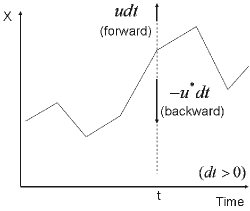
Figure 1: The forces acts on a Brownian particle at $t$. We set $dt>0$.

However, it is not straightforward to apply this interpretation to our stochastic model. Note that $U$ does not have explicit time dependence in Sekimoto’s definition. However, in our case, the energy of a Brownian particle in the backward process $U^{*}$ which is defined by ${\bf u}^{*}({\bf r},a,t)=-\nabla U^{*}({\bf r},a,t)$, has an explicit time dependence because of the time dependence of $\rho$ (See Eq. (12)). To apply Sekimoto’s procedure to our stochastic model, we introduce “averaged” thermodynamic quantities and discuss the thermodynamic relation for these quantities.

Note that the force which acts on a Brownian particle at $t$ is given by ${\bf u}({\bf X}(t),t)dt$ for the forward process and $-{\bf u}^{*}({\bf X}(t),t)dt$ for the backward process, as is shown in Fig. 1 ($dt>0$). Then we can introduce an averaged force which acts on a Brownian particle at $t$ as

$$\bar{\bf u}({\bf X}(t),a,t)dt={\bf b}({\bf X}(t),a,t)dt=\frac{{\bf u}({\bf X}(t),a,t)-{\bf u}^{*}({\bf X}(t),a,t)}{2}dt.$$ (22)

Correspondingly, the averaged energy is defined as

$$\bar{\bf u}({\bf X}(t),a,t)=-\nabla\bar{U}({\bf X}(t),a,t),~{}~{}~{}~{}\bar{U}({\bf X}(t),a,t)=\frac{U({\bf X}(t),a,t)-U^{*}({\bf X}(t),a,t)}{2}.$$ (23)

Following the discussion by Sekimoto, we implement the stochastic differentiation of $\bar{U}$ by using the Ito formula and obtain the thermodynamic relation for this averaged thermodynamic quantities as

$$d\bar{U}({\bf X}(t),a,t)=\delta\bar{Q}({\bf X}(t),a,t)+\delta\bar{\cal W}({\bf X}(t),a,t)+\delta Q_{J}({\bf X}(t),a,t),$$ (24)

where

$$\delta\bar{Q}({\bf X}(t),a,t) = \frac{\nabla U({\bf X}(t),a,t)-\nabla U^{*}({\bf X}(t),a,t)}{2}\circ d{\bf X}(t),$$ (25)

$$\delta\bar{\cal W}({\bf X}(t),a,t) = \frac{\partial_{a}U({\bf X}(t),a,t)-\partial_{a}U^{*}({\bf X}(t),a,t)}{2}\circ da,$$ (26)

$$\delta Q_{J}({\bf X}(t),a,t) = -\beta^{-1}\partial_{t}\ln\rho({\bf X}(t),a,t)dt$$ (27)

$$= -\beta^{-1}e^{\beta\bar{U}({\bf X}(t),a,t)}\nabla\cdot{\bf J}({\bf X}(t),a,t)dt.$$

Note that ${\bf X}(t)$ is a stochastic variable, we have to use the Ito formula instead of the Taylor expansion gardiner . In the derivation of the third equation, we used the macroscopic current defined from the Fokker-Planck equation as,

$$\partial_{t}\rho({\bf r},a,t)=\nabla\cdot{\bf J}({\bf r},a,t).$$ (28)

One can see that the first two terms on the r.h.s. of Eq. (24) already appear in Sekimoto’s thermodynamics relation, and $\delta\bar{Q}$ and $\delta\bar{\cal W}$ are interpreted as the averaged heat and the averaged work, respectively. However, the last term does not appear in Eq. (18).

In order to clarify the meaning of the new term $\delta Q_{J}$, let us consider the one-dimensional free Brownian motion. Then $\delta Q_{J}$ is calculated as

$$\delta Q_{J}(X(t),t)=-\beta^{-1}\frac{\partial_{x}J(X(t),t)}{\rho(X(t),t)}dt=\left(\frac{\beta^{-1}}{2t}-\frac{X^{2}(t)}{4t^{2}}\right)dt.$$ (29)

It is known that the expectation value of the position of a Brownian particle is given by $\langle X^{2}(t)\rangle=2\beta^{-1}t$, and one can easily see that $\delta Q_{J}$ vanishes in this case. Thus this term should be interpreted as another heat which a Brownian particle receives from the environment; when $X(t)$ moves slower than the average, $\delta Q_{J}$ is positive and a Brownian particle recieves heat, and vice versa. Apparently from Eq. (27), this heat appears only when $\rho$ has an explicit time dependence, that is, there is a non-vanishing macroscopic flow ${\bf J}$.

Note that, for the free Brownian motion, the energy of the forward process $U$ does not exist, but the averaged energy $\bar{U}$ is still finite. By using Eqs. (12) and (16), the averaged energy is calculated as

$$\bar{U}(X(t),t)=\frac{X^{2}(t)}{4t}+\frac{\beta^{-1}}{2}\ln(4\pi\beta^{-1}t).$$ (30)

Then the extended thermodynamic relation (24) for the free Brownian motion is explicitly given by

$$d\left(\frac{X^{2}(t)}{4t}+\frac{\beta^{-1}}{2}\ln(4\pi\beta^{-1}t)\right)=\left(\frac{\beta^{-1}}{2t}-\frac{X^{2}(t)}{4t^{2}}\right)dt+\frac{X(t)\circ dX(t)}{2t}.$$ (31)

The last term on the r.h.s. comes from $\delta\bar{Q}$, and there is no contribution from $\delta\bar{\cal W}$ in this case.

It should be noted that $\delta Q_{J}$ is re-expressed as,

$$\delta Q_{J}({\bf X}(t),a,t) = -\beta\nabla(e^{\beta\bar{U}({\bf X}(t),a,t)}{\bf J}({\bf X}(t),a,t))dt$$ (32)

$$-{\bf J}({\bf X}(t),a,t)\cdot{\bf b}({\bf X}(t),a,t)e^{\beta\bar{U}({\bf X}(t),a,t)}dt.$$

The first term on the r.h.s. is a total differentiation and may vanish for the total amount of the thermodynamic quantities. Note that ${\bf b}$ defined in Eq. (10) is the averaged force on a Brownian particle and the second term is expressed as the product of the macroscopic current ${\bf J}$ and the microscopic force ${\bf b}$. Remember that in the irreversible thermodynamics, the entropy production $\sigma$ is assumed to be given by the product of an irreversible current ${\bf J}_{irr}$ and the corresponding thermodynamic force ${\bf F}$,

$$\sigma={\bf J}_{irr}\cdot{\bf F}.$$ (33)

One can see that the form of the second term of Eq. (32) is very similar to this structure. In a quasi-static process, we may be possible to identify

$$\delta\bar{Q} = TdS,$$ (34)

$$\delta\bar{\cal W} = -PdV.$$ (35)

Then the extended thermodynamic relation is rewritten as

$$d\bar{U}=\delta Q_{J}+TdS-PdV.$$ (36)

This is very similar to the generalized thermodynamic relation discussed in the extended irreversible thermodynamics jou .

IV fluctuation theorem in stochastic processes

In this section, we will discuss the various fluctuation theorems in our stochastic model. Note that the fluctuation theorems based on the stochastic dynamics have already been discussed in several works seifert ; hatano . Differently from these works, our fluctuation theorems are expressed in terms of the averaged thermodynamic quantities introduced in the previous section.

Now we consider a set of a stochastic trajectory $\{{\bf X}(t)\}$ which is described by Eq. (1). Then, by calculating explicitly the total differentiation of $\bar{U}$ along this trajectory using the Ito formula gardiner , we find the following relation,

$$d\bar{U}({\bf X}(t),a,t)=(dU({\bf X}(t),a,t)-dU^{*}({\bf X}(t),a,t))/2=-\beta^{-1}d\ln\rho({\bf X}(t),a,t),$$ (37)

where

$$d\ln\rho({\bf X}(t),a,t) = [\partial_{t}+{\bf u}({\bf X}(t),a,t)\nabla+\beta^{-1}\nabla^{2}]\ln\rho({\bf X}(t),a,t)dt+\partial_{a}\ln\rho({\bf X}(t),a,t)\circ da$$ (38)

$$+\sqrt{2\beta^{-1}}\nabla\ln\rho({\bf X}(t),a,t)\cdot d{\bf W}(t).$$

Here the product in the inner product of the last term obeys the Ito definition gardiner .

Thus, for the evolution from $t_{0}$ to $t_{f}$, we have

$$\frac{\rho({\bf X}(t_{f}),a_{f},t_{f})}{\rho({\bf X}(t_{0}),a_{0},t_{0})}=e^{-\beta(\bar{U}({\bf X}(t_{f}),a_{f},t_{f})-\bar{U}({\bf X}(t_{0}),a_{0},t_{0}))}.$$ (39)

IV.1 Quasi-static change between two different stationary states

For the quasi-static process where we assume $\partial_{t}\rho({\bf r},a,t)\approx 0$, the extended thermodynamic relation is approximately given by

$$d\bar{U}({\bf X}(t),a,t)\approx\delta\bar{Q}({\bf X}(t),a,t)+\delta\bar{\cal W}({\bf X}(t),a,t).$$ (40)

Thus, from Eq. (39), the two stationary state are connected by the following relation,

$$\frac{\rho_{sta}({\bf X}(t_{f}),a_{f})}{\rho_{sta}({\bf X}(t_{0}),a_{0})}=e^{-\beta\sum_{i=0}^{f-1}(\delta\bar{Q}({\bf X}(t),a,t)+\delta\bar{\cal W}({\bf X}(t),a,t))}.$$ (41)

Clearly, there is no contribution from the macroscopic flow, $\delta Q_{J}$, in this case.

IV.2 Seifert relation

We consider a stochastic trajectory $\Gamma=\{{\bf X}_{0},{\bf X}_{1},\cdots,{\bf X}_{f}\}$ which is a solution of the stochastic difference equations (1), and introduce the corresponding time-reversed process denoted by $\Gamma^{\dagger}$. Then we consider the conditional probability which is defined by

$$P({\bf X}_{j},a_{j},t_{j}|{\bf X}_{i},a_{i},t_{i})=\frac{P(({\bf X}_{j},a_{j},t_{j})\cap({\bf X}_{i},a_{i},t_{i}))}{P({\bf X}_{i},a_{i},t_{i})}=\frac{\rho({\bf X}_{j},a_{j},t_{j})\rho({\bf X}_{i},a_{i},t_{i})}{\rho({\bf X}_{i},a_{i},t_{i})}=\rho({\bf X}_{j},a_{j},t_{j}),$$ (42)

where $\rho$ is the solution of the Fokker-Planck equation (5). Here we used that the process is Markovian. From Eq. (39), the r.h.s. of the above equation is given by

$$\rho({\bf X}_{j},a_{j},t_{j})=\rho({\bf X}_{i},a_{i},t_{i})e^{-\beta(\bar{U}({\bf X}_{j},a_{j},t_{j})-\bar{U}({\bf X}_{i},a_{i},t_{i}))}=e^{-\beta\bar{U}({\bf X}_{j},a_{j},t_{j})}.$$ (43)

The transition probability from an initial ${\bf X}_{0}$ to a final ${\bf X}_{f}$ along the stochastic trajectory $\Gamma$ is, finally, given by

$$P(\Gamma({\bf X}_{0},a_{0},t_{0};{\bf X}_{f},a_{f},t_{f}))$$ (44)

$$\equiv P({\bf X}_{f},a_{f},t_{f}|{\bf X}_{f-1},a_{f-1},t_{f-1})P({\bf X}_{f-1},a_{f-1},t_{f-1}|{\bf X}_{f-2},a_{f-2},t_{f-2})\cdots P({\bf X}_{1},a_{1},t_{1}|{\bf X}_{0},a_{0},t_{0})$$

$$= e^{-\beta[\sum_{i=0}^{f}\bar{U}({\bf X}_{i},a_{i},t_{i})-\bar{U}({\bf X}_{0},a_{0},t_{0})]}.$$

Similarly, the conditional probability for the inverse process is

$$P(\Gamma^{\dagger}({\bf X}_{0},a_{0},t_{0};{\bf X}_{f},a_{f},t_{f}))$$ (45)

$$\equiv P({\bf X}_{0},a_{0},t_{0}|{\bf X}_{1},a_{1},t_{1})P({\bf X}_{1},a_{1},t_{1}|{\bf X}_{2},a_{2},t_{2})\cdots P({\bf X}_{f-1},a_{f-1},t_{f-1}|{\bf X}_{f},a_{f},t_{f})$$

$$= e^{-\beta[\sum_{i=0}^{f}\bar{U}({\bf X}_{i},a_{i},t_{i})-\bar{U}({\bf X}_{f},a_{f},t_{f})]}.$$

Following the discussion by Seifert seifert , we introduce $R(\Gamma({\bf X}_{0},a_{0},t_{0};{\bf X}_{f},a_{f},t_{f}))$ as follows,

$$R(\Gamma({\bf X}_{0},a_{0},t_{0};{\bf X}_{f},a_{f},t_{f}))$$ (46)

$$= \ln\frac{P(\Gamma({\bf X}_{0}a_{0},,t_{0};{\bf X}_{f},a_{f},t_{f}))\rho({\bf X}_{0},a_{0},t_{0})}{P(\Gamma^{\dagger}({\bf X}_{0},a_{0},t_{0};{\bf X}_{f},a_{f},t_{f}))\rho({\bf X}_{f},a_{f},t_{f})}$$

$$= \ln\frac{\rho({\bf X}_{0},a_{0},t_{0})}{\rho({\bf X}_{f},a_{f},t_{f})}-\beta(\bar{U}({\bf X}_{f},a_{f},t_{f})-\bar{U}({\bf X}_{0},a_{0},t_{0}))$$

$$= \ln\frac{\rho({\bf X}_{0},a_{0},t_{0})}{\rho({\bf X}_{f},a_{f},t_{f})}-\beta\sum_{i=0}^{f-1}(\delta Q_{J}({\bf X}_{i},a_{i},t_{i})+\delta\bar{Q}({\bf X}_{i},a_{i},t_{i})+\delta\bar{\cal W}({\bf X}_{i},a_{i},t_{i})).$$

By using this, we can derive the exact relation,

$$\langle e^{-R(\Gamma({\bf X}_{0},a_{0},t_{0};{\bf X}_{f},a_{f},t_{f}))}\rangle$$ (47)

$$\equiv \int d^{3}{\bf X}_{0}d^{3}{\bf X}_{f}\langle P(\Gamma({\bf X}_{0},a_{0},t_{0};{\bf X}_{f},a_{f},t_{f}))\rho({\bf X}_{0},a_{0},t_{0})e^{-R(\Gamma({\bf X}_{0},a_{0},t_{0};{\bf X}_{f},a_{f},t_{f}))}\rangle_{W}$$

$$= 1,$$

were $\langle~{}\rangle_{W}$ means the average over possible trajectories fixing ${\bf X}_{0}$ at $t_{0}$ and ${\bf X}_{f}$ at $t_{f}$. Here we used the following relations,

$$\rho({\bf X}_{0},a_{0},t_{0}) = \int d^{3}{\bf X}_{f}\langle P(\Gamma^{\dagger}({\bf X}_{0},a_{0},t_{0};{\bf X}_{f},a_{f},t_{f}))\rho({\bf X}_{f},a_{f},t_{f})\rangle_{W},$$ (48)

$$\rho({\bf X}_{f},a_{f},t_{f}) = \int d^{3}{\bf X}_{0}\langle P(\Gamma({\bf X}_{0},a_{0},t_{0};{\bf X}_{f},a_{f},t_{f}))\rho({\bf X}_{0},a_{0},t_{0})\rangle_{W}.$$ (49)

This is the main result, leading to various fluctuation theorems.

The expression (47) corresponds to the relation discussed by Seifert seifert , but the expression of $R$ is different. Seifert gives the following representation for $R$,

$$R_{\mathrm{seifert}}=\ln\frac{\rho({\bf X}_{0},a_{0},t_{0})}{\rho({\bf X}_{f},a_{f},t_{f})}+\beta\sum_{i=0}^{f-1}{\bf u}_{i}\circ d{\bf X}_{i}=\ln\frac{\rho({\bf X}_{0},a_{0},t_{0})}{\rho({\bf X}_{f},a_{f},t_{f})}-\beta\sum_{i=0}^{f-1}\delta Q({\bf X}_{i},a_{i},t_{i}).$$ (50)

Thus our exact relation (47) is not equivalent to the Seifert relation.

The validity of the Seifert relation was numerically checked test . However, our result is also consistent with this numerical result. In test , the stationary state with fixed $a$ is considered. In this limited situation, our averaged quantities are reduced to

$$\delta Q_{J}=\delta\bar{\cal W}=0,~{}~{}~{}~{}\delta\bar{Q}=\delta Q.$$ (51)

Then our $R$ in (46) becomes equivalent to $R_{\mathrm{seifert}}$. In this sense, our result is still consistent with test .

IV.3 Jarzynski relation

It is easy to derive the relation corresponds to the Jarzynski relation jar from our relation (47). We consider that the evolution of a Brownian particle from one stationary state $\rho_{sta}({\bf r},a_{0})$, to the other one $\rho_{sta}({\bf r},a_{f})$. The stationary state is given by

$$\rho_{sta}({\bf r},a)=\frac{1}{Z_{sta}(a)}e^{-\beta U({\bf r},a)},$$ (52)

where $Z_{sta}(a)=\int d^{3}{\bf r}e^{-\beta U({\bf r},a)}$. Substituting it into Eq. (47), we obtain the Jarzynski relation of our stochastic model,

$$\langle e^{-\beta(U({\bf X}_{f},a_{f})-U({\bf X}_{0},a_{0})-\beta\sum_{i=0}^{f-1}(\delta Q_{J}({\bf X}_{i},a_{i},t_{i})+\delta\bar{Q}({\bf X}_{i},a_{i},t_{i})+\delta\bar{\cal W}({\bf X}_{i},a_{i},t_{i})))}\rangle=e^{-\beta\Delta F},$$ (53)

where

$$\Delta F=-\beta^{-1}\ln\frac{Z_{sta}(a_{f})}{Z_{sta}(a_{0})}.$$ (54)

IV.4 Komatsu-Nakagawa non-equilibrium steady state

Recently, the general expression of non-equilibrium steady state was derived in kn ; knst . The similar expression can be obtained in our stochastic model.

From Eq. (46), we have

$$P(\Gamma^{\dagger}({\bf X}_{0},a_{0},t_{0};{\bf X}_{f},a_{f},t_{f}))\rho({\bf X}_{f},a_{f},t_{f})$$ (55)

$$= P(\Gamma({\bf X}_{0},a_{0},t_{0};{\bf X}_{f},a_{f},t_{f}))\rho({\bf X}_{0},a_{0},t_{0})e^{-R(\Gamma({\bf X}_{0},a_{0},t_{0};{\bf X}_{f},a_{f},t_{f}))}.$$

Similarly, for the inverse process, we obtain

$$P(\Gamma({\bf X}_{0},a_{0},t_{0};{\bf X}_{f},a_{f},t_{f}))\rho({\bf X}_{0},a_{0},t_{0})$$ (56)

$$= P(\Gamma^{\dagger}({\bf X}_{0},a_{0},t_{0};{\bf X}_{f},a_{f},t_{f}))\rho({\bf X}_{f},a_{f},t_{f})e^{-R(\Gamma^{\dagger}({\bf X}_{0},a_{0},t_{0};{\bf X}_{f},a_{f},t_{f}))}.$$

By combining these equations, we have

$$P(\Gamma({\bf X}_{0},a_{0},t_{0};{\bf X}_{f},a_{f},t_{f}))\rho({\bf X}_{0},a_{0},t_{0})e^{-R(\Gamma({\bf X}_{0},a_{0},t_{0};{\bf X}_{f},a_{f},t_{f}))/2}$$ (57)

$$=P(\Gamma^{\dagger}({\bf X}_{0},a_{0},t_{0};{\bf X}_{f},a_{f},t_{f}))\rho({\bf X}_{f},a_{f},t_{f})e^{-R(\Gamma^{\dagger}({\bf X}_{0},a_{0},t_{0};{\bf X}_{f},a_{f},t_{f}))/2}.$$

This is re-expressed as

$$\rho({\bf X}_{f},a_{f},t_{f})=\rho({\bf X}_{0},a_{0},t_{0})\frac{\langle P(\Gamma({\bf X}_{0},a_{0},t_{0};{\bf X}_{f},a_{f},t_{f}))e^{-R(\Gamma({\bf X}_{0},a_{0},t_{0};{\bf X}_{f},a_{f},t_{f}))/2}\rangle_{W}}{\langle P(\Gamma^{\dagger}({\bf X}_{0},a_{0},t_{0};{\bf X}_{f},a_{f},t_{f}))e^{-R(\Gamma^{\dagger}({\bf X}_{0},a_{0},t_{0};{\bf X}_{f},a_{f},t_{f}))/2}\rangle_{W}}$$ (58)

Note that ${\bf X}_{f}$ and ${\bf X}_{0}$ are fixed parameters and independent of the average $\langle~{}\rangle_{W}$. This is essentially the same as the expression derived in kn (Eq. (10)), except for the definition of $R$. The quantity $\hat{\Theta}_{I}$ in kn , which corresponds to $R$ in our case, coincides with Eq. (46) when $\delta Q_{J}$ vanishes. That is, the Komatsu-Nakagawa non-equilibrium steady state is realized in our stochastic model only when there is no macroscopic flow.

V Concluding remarks

In this paper, we considered the stochastic model incorporating the forward process and the backward process in time. Following the strategy of Sekimoto seki , we constructed the thermodynamic relation for the “averaged” quantities of the forward and backward processes. Our thermodynamic relation is extended so that a term $\delta Q_{J}$ associated with a macroscopic flow appears. We further discussed the fluctuation theorems in our stochastic model and derived the new expressions with respect to the averaged quantities.

The new term $\delta Q_{J}$ can be expressed as the product of a macroscopic current and a force. This is the form expected from the extended irreversible thermodynamics. This term may have a relation to the excess heat discussed in oono

The consideration of the forward and backward stochastic equations is, in fact, well known in Nelson’s formulation of quantum mechanics, which is one of the hidden variable theories nelson . As a matter of fact, we can introduce a kind of a wave function even in the classical Brownian motion and it is possible to interpret the fluctuation theorems in terms of the phase of the wave function. This will be reported in another work.

In this work, we discussed the stochastic equation of motion without inertial terms under a Gaussian white noise. It is also interesting to extend our discussion to the equations with inertial terms, memory effects and colored noise. In such a situation, it may be possible to investigate the dynamics of the pre-equilibrium state as is discussed in kk . Moreover, if our discussion is applicable to relativistic Brownian motion hanggi , we can investigate the thermodynamic relation in relativistic systems.

T. Koide acknowledges useful comments by G. S. Denicol. This work was (financially) supported by the Helmholtz International Center for FAIR within the framework of the LOEWE program (Landesoffensive zur Entwicklung Wissenschaftlich- Okonomischer Exzellenz) launched by the State of Hesse.

References

• (1) K. Sekimoto, J. Phys. Soc. Jpn, 66, 1234 (1997); Stochastic Energetics (Iwanami, 2004, in Japanese).
• (2) U. Seifert, Phys. Rev. Lett. 95, 040602 (2005).
• (3) C. Jarzynski, J. Stat. Phys. 98, 77 (2000).
• (4) T. S. Komatsu and N. Nakagawa, Phys. Rev. Lett. 100, 030601 (2008).
• (5) C. W. Gardiner, Handbook of Stochastic Methods, (Springer-Verlag, Berlin, 1990).
• (6) See, for example, K. Sekimote and S. Sasa, J. Phys. Soc. Jpn 66, 3326 (1997); K. Sekimoto, F. Takagi and T. Hondou, Phys. Rev. E 62, 7759 (2000); H. Kamegawa, T. Hondou and F. Takagi, Phys. Rev. Lett. 80, 5251 (1998).
• (7) D. Jou, J. Casas-Vázquez and G. Lebon, 1988 Rep. Prog. Phys. 51 1105; 1999 Rep. Prog. Phys. 62 1035.
• (8) T. Hatano, Phys. Rev. E60, R5017 (1999).
• (9) A. Gomez-Marin and I. Pagonabarraga, Phys. Rev. E74, 061113 (2006).
• (10) T. S. Komatsu, N. Nakagawa, S. Sasa and H. Tasaki, J. Stat. Phys. 134, 401 (2009).
• (11) Y. Oono and M. Paniconi, Prog. Theor. Phys. Suppl. 130, 29 (1998).
• (12) E. Nelson, Phys. Rev. 150, 1079 (1966); K. Yasue and J. C. Zambrini, Ann. Phys. 159, 99 (1985).
• (13) T. Kodama, H.-T. Elze, C. E. Aguiar and T. Koide, Euro. Phys. Lett. 70, 439 (2005); T. Kodama and T. Koide, Eur. Phys. J A40, 289 (2009).
• (14) J. Dunkel and P. Hänggi, Phys. Rep. 471 1, 2009.