Abstract

Relativistic Continuum Random Phase Approximation (CRPA) is used to investigate collective excitation phenomena in several spherical nuclei along the periodic table. We start from relativistic mean field calculations based on a covariant density functional with density dependent zero range forces. From the same functional an effective interaction is obtained as the second derivative with respect to the density. This interaction is used in relativistic continuum-RPA calculations for the investigation of isoscalar monopole, isovector dipole and isoscalar quadrupole resonances of spherical nuclei. In particular we study the low-lying E1 strength in the vicinity of the neutron evaporation threshold. The properties of the resonances, such as centroid energies and strengths distributions are compared with results of discrete RPA calculations for the same model as well as with experimental data.

Continuum Random Phase Approximation for Relativistic Point Coupling Models

PACS numbers: 21.30.Fe, 21.60.Jz, 21.65.+f, 21.10.-k

1 Introduction

Density functional theory (DFT) provides a very successful description of nuclei all over the periodic table. Based on relatively simple functionals, which are adjusted in a phenomenological way to the properties of infinite nuclear matter and a few finite nuclei, this theory allows a highly accurate reproduction of many nuclear structure data, such as binding energies, radii, deformation parameters of finite nuclei and their dependence on mass number and isospin. In addition to these static properties, one can use the nuclear response to external multipole fields to investigate the dynamics of such systems. In the framework of time dependent density functional theory, this response can be calculated from the linearized Bethe Salpeter equation using an effective interaction derived from the same functional.

A very successful scheme of this type is covariant density functional theory (CDFT). It is based on Lorentz invariance, connecting in a consistent way the spin and spatial degrees of freedom of the nucleus. Therefore, it needs only a relatively small number of parameters which are adjusted to reproduce a set of bulk properties of spherical closed-shell nuclei. Numerous works have shown that observations involving both ground state and excited state phenomena, can be nicely interpreted in a relativistic framework.

The most popular applications of this type are based on the Walecka model [1], where the nucleus is described as a system of Dirac nucleons interacting with each other via the exchange of virtual mesons with finite mass and the electromagnetic field through an effective Lagrangian. In the mean field approximation this yields to various contributions to the nuclear self energy depending on the quantum numbers of these mesons. Early investigations have shown that this simple ansatz is not able to describe the incompressibility of infinite nuclear matter nor the surface properties of finite nuclei such as nuclear deformations. For that reason, a medium dependence has been introduced by including nonlinear meson self-interaction terms in the Lagrangian [2].

Several very successful phenomenological RMF interactions of this type have been adopted, as for instance the popular set NL3 [3]. Closer to the concept of density functional theory are models with an explicit density dependence for the meson nucleon couplings. This density dependence can be calculated from first principles in a microscopic Dirac-Brueckner scheme [4] or it can be adjusted in a completely phenomenological way to properties of finite nuclei [5, 6].

One of the advantages of density functional theory is the fact that with a proper choice of the parameters the success of RMF for nuclear ground states ensures also a good basis upon which one can apply time-dependent density functional theory to study nuclear excitations. In order to investigate the dynamic behavior of the nuclear system, one considers oscillations around the self-consistent static solution. This can be done by solving the time dependent relativistic mean field equations (TDRMF) [7] or, in the limit of small amplitudes, by using the relativistic random phase approximation (RRPA) [8]. The corresponding eigen modes can be determined either by diagonalizing the RRPA equation in an appropriate basis or by solving the linear response equations in a time-dependent external field. This requires a matrix inversion for given frequency $\omega$.

These two methods lead in principle to exactly identical results. There are, however, cases where one of them is clearly preferable. The proper treatment of the coupling to the continuum is such a case, which can be solved in a very elegant way, by the solution of the Bethe Salpeter equation within the response formalism.

We recall that the spectrum of the Dirac equations has a discrete and a continuous part. For the ground state properties of the nucleus, one needs only the single particle wave functions of the occupied orbitals in the Fermi sea. They are either determined by solving the corresponding differential equations in $r$-space or by expansion in an appropriate basis, given for for instance by a finite number of eigenfunctions of a harmonic oscillator [9] or of a Saxon-Woods potential in a finite box [10]. For the bound states both methods yield the same solutions with high accuracy. However, this is no longer true for the states in the continuum. Here we have, in the first case scattering solutions in $r$-space for each energy with proper boundary conditions, while in the second case, a finite number of discrete eigenstates which depend strongly on the dimension of the expansion. They provide only a basis and have little to do with physics.

These discrete eigenstates lead to a finite number of $ph$-configurations for the solution of response equations. with a discrete spectrum. They provide us with the so called spectral representation of the response function in contrast to the continuum representation, where the exact scattering states with the proper boundary conditions are used at each energy.

Self-consistent relativistic RPA (RRPA) calculations have a long history. The early investigations in the eighties [11, 13, 14, 15] were based on the Walecka model with linear meson-nucleons couplings. They were able to describe the low-lying negative-parity excitations in ¹⁶O by the method of matrix diagonalization [11], isoscalar giant resonances in light and medium nuclei [13] by the solution of the linear response equation in the spectral representation, and the longitudinal response for quasi-elastic electron scattering with a proper treatment of the continuum.

The first RRPA calculations based on non-linear models were carried out in the spectral representation including only normal particle-hole ($ph$) pairs with particles above the Fermi energy and holes in the Fermi sea. This seemed to be a reasonable approximation, since the configurations formed by particles in the Dirac sea and holes in the Fermi sea ($ah$-pairs) are more than 1.2 GeV away from the normal $ph$-pairs. Indeed, a proper coupling to the Dirac sea and current conservation was neglected in these investigations. They showed considerable deviations from the results obtained form time-dependent RMF-calculations with the same Lagrangian, particularly for isoscalar excitations [16]. A fully self-consistent treatment with current conservation requires the inclusion of a very large number of $ah$-pairs connected with a considerable numerical effort. Most of the very successful applications of RRPA theory based on non-linear meson-nucleon coupling models in the last ten years have been carried out in this way [17, 18, 19, 20, 21].

There are also relativistic continuum RPA calculations based on the non-spectral representation of the response function using the single particle Green’s function in the continuum with proper boundary conditions [14]. These calculations are done for meson exchange forces with finite range. The early investigations were based on linear models. Later on the method was generalized to include non-linear coupling terms between the mesons [22]. This leads to a a more sophisticated density dependence which is crucial for a realistic description of giant resonances in nuclei [22, 23].

Of course, because of the finite range of the effective force these models are relatively complicated not only for static applications to triaxially deformed or rotating nuclei, but also for investigations of nuclear dynamics, such as the solution of the relativistic RPA or linear response equations for the description of excited states. In particular one needs simpler forces for applications going beyond the mean field approach such as Particle Vibrational Coupling (PVC) [24] or configuration mixing calculations in the framework of the Generator Coordinate Method (GCM) [25]. Therefore over the years several attempts have been made to develop relativistic point coupling (PC) models with forces of zero range [26], in analogy to non-relativistic Skyrme-functionals. but only recently parameter sets have been found, which are comparable in quality to the density dependent meson-exchange models [27, 28].

PC models do not contain mesonic degrees of freedom and are therefore closer to the philosophy of the density functional theory. Their essential advantage is of course the fact that the zero range of the effective interaction reduces considerably the numerical effort in practical applications. Because of their simplicity they are nowadays much used in many complex calculations going beyond the mean field approach [24, 25]. However, so far they have not been used much for the dynamic investigations and it is only quite recently that a code has been developed to diagonalize the RPA equations for relativistic Point Coupling models [21] and it has been shown that this latter approach reproduces excitation and collective phenomena, in particular Giant Multipole Resonances, with a quality comparable to that of standard finite-range forces.

This manuscript is devoted to an investigation of relativistic point coupling models with an exact treatment of the coupling to the continuum. The relativistic response equations are solved both in the continuum and in the spectral representation and the corresponding results are compared. We use the Lagrangian PC-F1 [27], which is capable of reproducing a wide range of experimental data.

The paper is organized in the following way: In Sec. 2 we present the main characteristics of the point coupling RMF theory, while the relativistic RPA equations are derived in Sec. 3. The proper treatment of the continuum in connection with point coupling models is discussed in Sec. 4 and in Sec. 5 we finally present applications of this method for the spectra of in spherical nuclei. In particular we calculate the strength function of Isoscalar and Isovector Giant Resonances as well as their contributions to their respective energy weighted sum rules. The results are summarized in Sec. 6.

2 Relativistic mean field theory of zero range.

As in all the relativistic models, the nucleons are described as point like Dirac particles. In contrast to the Walecka model, however, where these particles interact by the exchange of effective mesons with finite mass, point coupling models [26] neglect mesonic degrees of freedom and consider only interactions with zero range. In principle, these models are similar to the Nambu Jona-Lasinio model [30] used extensively in hadron physics. There is, however, an important difference: in order to obtain a satisfactory description of the nuclear surface properties one needs gradient terms in the Lagrangian simulating a finite range of the interaction.

A general point-coupling effective Lagrangian is constructed to be consistent with the underlying symmetries of $QCD$ (e.g., Lorentz covariance, gauge invariance, and chiral symmetry). It should in principle contain every possible term, allowed by these symmetries, but at the same time should also be described by the least possible number of parameters in order to give a quantitative solution.

In this work we use the point coupling Lagrangian introduced by Buervenich et al. in Ref. [27]. It presents an expansion in powers of the nucleon scalar, vector and isovector-vector densities. The Lagrangian

$$\mathcal{L}=\mathcal{L}_{\mathrm{free}}+\mathcal{L}_{\mathrm{4f}}+\mathcal{L}_{\mathrm{hot}}+\mathcal{L}_{\mathrm{der}}+\mathcal{L}_{\mathrm{em}}$$ (1)

consists of the term for free nucleons:

$$\mathcal{L}_{\mathrm{free}}=\bar{\psi}(i\gamma_{\mu}\partial^{\mu}-m_{N})\psi,$$ (2)

the term for normal four-fermion interactions

$$\mathcal{L}_{\mathrm{4f}}= -\frac{\alpha_{S}}{2}(\bar{\psi}\psi)(\bar{\psi}\psi)-\frac{\alpha_{V}}{2}(\bar{\psi}\gamma_{\mu}\psi)(\bar{\psi}\gamma^{\mu}\psi)$$ (3)

$$-\frac{\alpha_{TS}}{2}(\bar{\psi}\vec{\tau}\psi)(\bar{\psi}\vec{\tau}\psi)-\frac{\alpha_{TV}}{2}(\bar{\psi}\vec{\tau}\gamma_{\mu}\psi)(\bar{\psi}\vec{\tau}\gamma^{\mu}\psi),$$

the term for higher order terms leading in mean field approximation to a density dependence

$$\mathcal{L}_{\mathrm{hot}}=-\frac{\beta_{S}}{3}(\bar{\psi}\psi)^{3}-\frac{\gamma_{S}}{4}(\bar{\psi}\psi)^{4}-\frac{\gamma_{V}}{4}[(\bar{\psi}\gamma_{\mu}\psi)(\bar{\psi}\gamma^{\mu}\psi)]^{2},$$ (4)

the term containing derivative terms which simulate in a simple way the finite range of the forces:

$$\mathcal{L}_{\mathrm{der}} =-\frac{\delta_{S}}{2}(\partial_{\mu}\bar{\psi}\psi)(\partial^{\mu}\bar{\psi}\psi)-\frac{\delta_{V}}{2}(\partial_{\mu}\bar{\psi}\gamma_{\nu}\psi)(\partial^{\mu}\bar{\psi}\gamma^{\nu}\psi)$$

$$-\frac{\delta_{TS}}{2}(\partial_{\mu}\bar{\psi}\vec{\tau}\psi)(\partial^{\mu}\bar{\psi}\vec{\tau}\psi)-\frac{\delta_{TV}}{2}(\partial_{\mu}\bar{\psi}\vec{\tau}\gamma_{\nu}\psi)(\partial^{\mu}\bar{\psi}\vec{\tau}\gamma^{\nu}\psi)$$ (5)

and finally the electro-magnetic part

$$\mathcal{L}_{\mathrm{em}}=-\frac{1}{4}F_{\mu\nu}F^{\mu\nu}-\frac{e}{2}(1-\tau_{3})A_{\mu}\bar{\psi}\gamma^{\mu}\psi.$$ (6)

In these equations, $\psi$ represents the nucleon spinors. The subscripts $S$ and $V$ are attributed to scalar and vector fields, while the subscript $T$ is attributed to isovector fields. As usual, vectors in isospin space are denoted by arrows, where symbols in bold indicate vectors in ordinary three-dimensional coordinate space.

From this Lagrangian and the corresponding energy momentum tensor we can derive a relativistic energy density functional. It has the form:

$$\mathcal{E}_{\mathrm{RMF}}[\hat{\rho},t]=\int d^{3}r~{}{H(\bm{r},t}),$$ (7)

where the energy density

$$H(\bm{r},t)=H_{\mathrm{kin}}(\bm{r},t)+H_{\mathrm{int}}(\bm{r},t)+H_{\mathrm{em}}(\bm{r},t)$$ (8)

consists of a kinetic part

$$H_{\mathrm{kin}}(\bm{r},t)=\sum_{i}^{A}\,{\bar{\psi}_{i}(\bm{r},t)\left(\bm{\alpha}\bm{p}+\beta m-m\right)\psi_{i}(\bm{r},t)},$$ (9)

an interaction part

$$H_{\mathrm{int}}(\bm{r},t) =\frac{\alpha_{S}}{2}\rho_{S}^{2}+\frac{\beta_{S}}{3}\rho_{S}^{3}+\frac{\gamma_{S}}{4}\rho_{S}^{4}+\frac{\delta_{S}}{2}\rho_{S}\Delta\rho_{S}$$

$$+\frac{\alpha_{V}}{2}j_{\mu}j^{\mu}+\frac{\gamma_{V}}{4}(j_{\mu}j^{\mu})^{2}+\frac{\delta_{V}}{2}j_{\mu}\triangle j^{\mu}$$ (10)

$$+\frac{\alpha_{TV}}{2}\vec{j}_{TV}^{\mu}\cdot\vec{j}_{TV\mu}+\frac{\delta_{TV}}{2}\vec{j}_{TV}^{\mu}\cdot\triangle(\vec{j}_{TV})_{\mu}$$

and an electromagnetic part

$$H_{\mathrm{em}}(\bm{r},t)=\frac{1}{4}F_{\mu\nu}F^{\mu\nu}-F^{0\mu}\partial_{0}A_{\mu}+eA_{\mu}j_{p}^{\mu}.$$ (11)

The interaction part depends on the local densities:

$$\rho_{S}(\bm{r},t) =\sum_{i}^{A}\bar{\psi}_{i}(\bm{r},t)\psi_{i}(\bm{r},t),$$ (12)

$$\rho_{V}(\bm{r},t) =\sum_{i}^{A}\bar{\psi}_{i}(\bm{r},t)\gamma_{0}\psi_{i}(\bm{r},t),$$ (13)

$$\rho_{TS}(\bm{r},t) =\sum_{i}^{A}\bar{\psi}_{i}(\bm{r},t)\tau_{3}\psi_{i}(\bm{r},t),$$ (14)

$$\rho_{TV}(\bm{r},t) =\sum_{i}^{A}\bar{\psi}_{i}(\bm{r},t)\tau_{3}\gamma_{0}\psi_{i}(\bm{r},t)$$ (15)

and currents

$$j_{V}^{\mu}(\bm{r},t) =\sum_{i}\bar{\psi}_{i}(\bm{r},t)\gamma^{\mu}\psi_{i}(\bm{r},t),$$ (16)

$$\vec{j}_{TV}^{\mu}(\bm{r},t) =\sum_{i}\bar{\psi}_{i}(\bm{r},t)\vec{\tau}\gamma^{\mu}\psi_{i}(\bm{r},t).$$ (17)

As in all relativistic mean field models, the no-sea approximation is used in the calculations of the nuclear densities by summing only over the single-particle states with energies in the Fermi sea. Vacuum polarization effects are not taken into account explicitly but only in a global way by the correct choice of the Lagrangian parameters. All interactions in the Lagrangian (1) are then expressed in terms of the corresponding local densities

Many effects, which go beyond mean field, seem to be neglected on the classical level, such as Fock-terms, vacuum polarization, short range Brueckner correlations etc. However, the coupling constants of the method are adjusted to experimental data, which, of course, contain all these effects and many more. Therefore these effects are not neglected. On the contrary, they are taken into account in an effective way. This concept of RMF methods is therefore equivalent to that of density functional theory.

The time-dependent variational principle

$$\delta\int\left\{i\langle\Phi(t)|\frac{\partial}{dt}|\Phi(t)\rangle-E[\hat{\rho}(t)]\right\}\,dt=0$$ (18)

allows us to derive from the energy density functional $E[\hat{\rho}]$ an equation of motion for the time-dependent relativistic single particle density:

$$\hat{\rho}(\mathbf{r},\mathbf{r^{\prime}},t)=\sum_{i}^{A}|\psi_{i}(\mathbf{r},t)\rangle\langle\psi_{i}(\mathbf{r^{\prime}},t)|,$$ (19)

which has the form

$$i\partial_{t}\hat{\rho}(t)=[\hat{h}(\hat{\rho}(t)),\hat{\rho}(t)].$$ (20)

The self energy, i.e. the single particle hamiltonian $\hat{h}(\hat{\rho}(t))$ is obtained as the functional derivative of the energy density functional with respect to the relativistic density matrix:

$$\hat{h}=\frac{\delta E[\hat{\rho}]}{\delta\hat{\rho}}.$$ (21)

This yields the Dirac hamiltonian:

$$\hat{h}=\bm{\alpha}[-i\bm{\nabla}-\bm{V}(\bm{r},t)]+V(\bm{r},t)+\beta(m+S(\bm{r},t))$$ (22)

with the self-consistent scalar and vector potentials

$$S(\bm{r},t) =\Sigma_{S}(\bm{r},t)+\vec{\tau}\cdot\vec{\Sigma}_{TS}(\bm{r},t),$$ (23)

$$V^{\mu}(\bm{r},t) =\Sigma^{\mu}(\bm{r},t)+\vec{\tau}\cdot\vec{\Sigma}^{\mu}_{T}(\bm{r},t).$$ (24)

The nucleon isoscalar-scalar, isovector-scalar, isoscalar-vector and isovector-vector self-energies are density dependent and defined by the following relations:

$$\Sigma_{S} =\alpha_{S}\rho_{S}+\beta_{S}\rho_{S}^{2}+\gamma_{S}\rho_{S}^{3}-\delta_{S}\Delta\rho_{S},$$ (25)

$$\vec{\Sigma}_{TS} =\alpha_{TS}\rho_{TS}-\delta_{TS}\Delta\rho_{TS},$$ (26)

$$\Sigma^{\mu} =\alpha_{V}\rho_{V}+\gamma_{V}\rho_{V}^{3}-\delta_{V}\Delta\rho_{V}-eA^{\mu}\frac{1-\tau_{3}}{2},$$ (27)

$$\vec{\Sigma}^{\mu}_{T} =\alpha_{TV}\rho_{TV}-\delta_{TV}\Delta\rho_{TV}.$$ (28)

Here we have neglected retardation effects, i.e. second derivatives with respect to the time for the various densities.

In the static limit we have

$$[\hat{h}(\hat{\rho}),\hat{\rho}]=0,$$ (29)

thus the static density $\hat{\rho}_{0}$ is obtained from the solution of the self-consistent Dirac equations upon all the nucleons with eigenvalues $\varepsilon_{k}$ and eigenfunctions $\psi_{k}(r)$:

$$\hat{h}|\psi_{k}(\bm{r})\rangle=\varepsilon_{k}|\psi_{k}(\bm{r})\rangle.$$ (30)

For spherical symmetry the spinors have the form:

$$|\mathcal{\psi}_{n\kappa\,m}(\bm{r})\rangle=\frac{1}{r}{\binom{f_{n\kappa}(r)\mathcal{Y}_{\kappa\,m}(\Omega)}{ig_{n\kappa}(r)\mathcal{Y}_{\bar{\kappa}\,m}(\Omega)}}.$$ (31)

The subscripts $n$, $\kappa$ and $m$ are principal and angular momentum quantum numbers; $\kappa=\mp(j+\frac{1}{2})$ for $j=l\pm\frac{1}{2}$, where $j$ and $l$ are the total and the orbital angular momenta of the nucleon. As usual, $m$ is the $z$ component of the total angular momentum. The spherical spinors $\mathcal{Y}_{\kappa\,m}(\Omega)$ are given in terms of spherical harmonics $Y_{lm_{l}}(\Omega)$ and Pauli spinors $\chi_{m_{s}}$ as:

$$\mathcal{Y}_{\kappa\,m}(\Omega)=\sum_{m_{l}m_{s}}(\frac{1}{2}m_{s}lm_{l}|jm)Y_{lm_{l}}(\Omega)\chi_{m_{s}},$$ (32)

while the functions $f_{i}(r)$ and $g_{i}(r)$ satisfy the static radial Dirac equations:

$$\left(\begin{array}[c]{cc}V+S&-\partial_{r}+\frac{\kappa}{r}\\ \partial_{r}+\frac{\kappa}{r}&V-S-2m\end{array}\right)\left(\begin{array}[c]{c}f_{i}(r)\\ g_{i}(r)\end{array}\right)=\left(\begin{array}[c]{c}f_{i}(r)\\ g_{i}(r)\end{array}\right)\varepsilon_{i}.$$ (33)

Coupling const.	PC-F1
$\alpha_{S}$	-14.	935894
$\delta_{S}$	-0.	634576
$\alpha_{V}$	10.	098025
$\delta_{V}$	-0.	180746
$\alpha_{TS}$	0.	0
$\delta_{TS}$	0.	0
$\alpha_{TV}$	1.	350268
$\delta_{TV}$	-0.	063680
$\beta_{S}$	22.	994736
$\gamma_{S}$	-66.	769116
$\gamma_{V}$	-8.	917323

Table 1: The coupling constants in the parameter set PC-F1 resulting from the fitting procedure in Ref. [27]. The units are [fm^-2] for the constants $\alpha$ of the quadratic terms, [fm^-4] for the constants $\delta$ of the derivative terms, [fm^-5] for the constants $\beta$ of the cubic terms, and [fm^-8] for the constants $\gamma$ of the quartic terms in the Lagrangian.

The point coupling Lagrangian used in this work contains eleven coupling constants. Based on an extensive multi parameter $\chi^{2}$ minimization procedure, Bürvenich et al. [27] have adjusted the parameter set $PC$-$F1$ to reproduce ground state properties of infinite nuclear matter and spherical doubly closed shell nuclei. This set is listed in Table 1 and it has been tested in the calculation of many ground state properties of spherical and deformed nuclei all over the periodic table. The results are very well comparable with reasonable effective meson-exchange interactions.

The nuclear ground state is defined as the equilibrium point of the functional (7), thus, is associated with the density which minimizes $E_{\mathrm{RMF}}[\hat{\rho}]$. Furthermore, small oscillations around this equilibrium point correspond to the vibrational nuclear states. They are usually described within the harmonic approximation, that is, using linear response theory. In nuclear physics, this is the so called Random Phase Approximation (RPA) which has been already mentioned in our discussion and will be described in more detail in the next section.

3 Relativistic RPA formalism

Under the influence of an external field $F(\omega)$ oscillating with the frequency $\omega$ the nucleus is excited. The cross section of this process is proportional to the strength function:

$$S(\omega) =-\frac{1}{\pi}\operatorname{Im}\sum_{\alpha\beta\alpha^{\prime}\beta^{\prime}}F_{\alpha\beta^{\ast}}R_{\alpha\beta\alpha^{\prime}\beta^{\prime}}(\omega)F_{\alpha^{\prime}\beta^{\prime}}$$

$$:=-\frac{1}{\pi}\operatorname{Im}R_{FF}(\omega),$$ (34)

where $F_{\alpha\beta}$ is the operator inducing the reaction and $R_{\alpha\beta\gamma\delta}(\omega)$ is the response function which, in an arbitrary representation indicated by the Greek indices $\alpha,\beta,\ldots$ (e.g. the ($\bm{r},s)$-representation) is defined as:

$$R_{\alpha\beta\alpha^{\prime}\beta^{\prime}}(\omega)=\sum\limits_{\nu}\left\{\frac{\langle 0|a_{\beta}^{+}a_{\alpha}|\nu\rangle\langle\nu|a_{\alpha^{\prime}}^{+}a_{\beta^{\prime}}|0\rangle}{\omega-E_{\nu}+E_{0}+i\eta}\right.-\left.\frac{\langle\nu|a_{\beta}^{+}a_{\alpha}|0\rangle\langle 0|a_{\alpha^{\prime}}^{+}a_{\beta^{\prime}}|\nu\rangle}{\omega+E_{\nu}-E_{0}+i\eta}\right\}.$$ (35)

The imaginary part $i\eta$ is infinitesimal and is introduced in order to fulfill the proper boundary conditions and to prevent $R(\omega)$ from diverging at $\omega=E_{\nu}-E_{0}$. We use here the response derived from the retarded Green’s functions as defined in Ref. [53]

In the independent particle model, $|0\rangle$ is the Slater determinant of the ground state, formed by the self-consistent solutions of the Dirac equation (30) and $|\nu\rangle=a_{p}^{+}a_{h}|0\rangle$ are $ph$-states, while $E_{0}$ and $E_{\nu}$ are the corresponding energies. In the basis $|k\rangle$, where the single particle hamiltonian (22) is diagonal we obtain the free response function:

$$R_{klk^{\prime}l^{\prime}}^{\,0}(\omega)=\frac{n_{k}-n_{l}}{\omega-\varepsilon_{k}+\varepsilon_{l}+i\eta}\delta_{kk^{\prime}}\delta_{ll^{\prime}}$$ (36)

with the occupation factors:

$$n_{k}=\langle 0|a_{k}^{+}a_{k}|0\rangle=\left\{\begin{array}[c]{ll}1&\text{for hole states with }\varepsilon_{k}\leq\varepsilon_{F}\\ 0&\text{for particle states with }\varepsilon_{k}>\varepsilon_{F}\end{array}\right.$$ (37)

The full response of Eq. (35) contains the transition densities:

$$\rho_{\alpha\beta}^{\nu}=\langle 0|a_{\beta}^{+}a_{\alpha}|\nu\rangle.$$ (38)

They can be deduced from the time-dependent density matrix in Eq. (19), which is derived from the variational principle in Eq. (18).

In the small amplitude limit one uses the linear response approximation to obtain the full response $R(\omega)$ of Eq. (35) as the solution of the linearized Bethe-Salpeter equation:

$$R_{\alpha\beta\alpha^{\prime}\beta^{\prime}}(\omega)=R_{\alpha\beta\alpha^{\prime}\beta^{\prime}}^{\,0}(\omega)+\sum_{\gamma\delta\gamma^{\prime}\delta^{\prime}}\,\,R^{0}_{\alpha\beta\gamma\delta}(\omega)V_{\gamma\delta\gamma^{\prime}\delta^{\prime}}^{\text{ph}}R_{\gamma^{\prime}\delta^{\prime}\alpha^{\prime}\beta^{\prime}}(\omega).$$ (39)

The relativistic residual interaction is found as the second derivative of the energy density functional (7) with respect to the density matrix

$$V_{\alpha\beta\alpha^{\prime}\beta^{\prime}}^{\text{ph}}=\frac{\delta^{2}E[\hat{\rho}]}{\delta\hat{\rho}_{\alpha\beta}\delta\hat{\rho}_{\alpha^{\prime}\beta^{\prime}}}.$$ (40)

Once again, we have neglected retardation and this effective interaction has to be calculated at the static density.

In a short hand notation the response equation (39) has the formal solution

$$R(\omega)=(1-R^{\,0}(\omega)V^{\text{ph}})^{-1}R^{\,0}(\omega)$$ (41)

or introducing the inverse of $R^{\,0}$ we have

$$R(\omega)=\frac{1}{R^{\,0}(\omega)^{-1}-V^{\text{ph}}}$$ (42)

The evaluation of the strength function (34) requires therefore three steps. The starting point is the calculation of the free response function $R^{\,0}(\omega)$. In the next step one determines the interaction $V^{\text{ph}}$ and finally one solves the response equation by the inversion (41). In details there are several methods to proceed. In particular one can choose various basis sets to solve these equations.

a) As we have seen in Eq. (36) the free response has a particularly simple form in the basis of Dirac spinors (Dirac basis) diagonalizing the self-consistent mean field equation (30). This is in particular simple for cases where the Dirac equation is solved in a discrete basis, as for instance the oscillator basis [9] or in a Saxon Woods basis [10] determined by the solution of the Dirac equation in a box with finite size. However, the simplicity in the calculation of $R^{\,0}(\omega)$ is compensated by the computational effort required in the next steps. First we have to calculate a large number of matrix elements for the interaction (40) in the basis of the corresponding $ph$-states and in a second step the matrix $(1-R^{\,0}(\omega)V^{\text{ph}})$ has to be inverted for each value of the frequency $\omega$. In general the number of single particle states is rather large and this leads to a huge number of $ph$-states, requiring considerable computational sources, not only in memory but also in computer time. This is in particular a problem in the case of deformed nuclei. By this reason this method can only be used successfully for light spherical nuclei, where the number of $ph$-states is limited.

b) The inversion is particular simple in the RPA-basis. Inserting expression (36) into Eq. (42) we find that the response function is equivalent to the resolvent of the RPA matrix

$$R^{\,0}(\omega)^{-1}-V^{\text{ph}}=\omega-\left(\begin{array}[c]{cc}A&B\\ -B^{\ast}&-A^{\ast}\end{array}\right)$$ (43)

where

$$A_{php^{\prime}h^{\prime}} =(\varepsilon_{p}-\varepsilon_{h})\delta_{pp^{\prime}}\delta_{hh^{\prime}}+V_{php^{\prime}h^{\prime}}^{\text{ph}},\text{\ }$$ (44)

$$B_{php^{\prime}h^{\prime}} =V_{phh^{\prime}p^{\prime}}^{\text{ph}}$$ (45)

Of course, the calculation of this matrix requires the same numerical effort as the evaluation of $V^{\text{ph}}$ in the Dirac basis discussed above. However there exist standard routines for the diagonalization of the RPA-matrix

$$\left(\begin{array}[c]{cc}A&B\\ -B^{\ast}&-A^{\ast}\end{array}\right)\left(\begin{array}[c]{c}X\\ Y\end{array}\right)_{\mu}=\left(\begin{array}[c]{c}X\\ Y\end{array}\right)_{\mu}\Omega_{\mu}$$ (46)

and this diagonalization has to be carried out only once, whereas the inversion of the response equation has to be done for each value of the frequency $\omega$. In the RPA-basis given by the eigenvectors $|\mu\rangle$ the reduced response function defined in Eq. (52) has a particular simple form

$$R_{cc^{\prime}}(\omega)={\sum\limits_{\mu>0}}\frac{\langle 0|Q_{c}^{{\dagger}}|\mu\rangle\langle\mu|Q_{c^{\prime}}|0\rangle}{\omega-\Omega_{\mu}+i\eta}-\frac{\langle\mu|Q_{c}^{{\dagger}}|0\rangle\langle 0|Q_{c^{\prime}}|\mu\rangle}{\omega+\Omega_{\mu}+i\eta}.$$ (47)

Using

$$\langle 0|F|\mu\rangle=\sum\limits_{ph}F_{ph}(X_{ph}^{\mu}+Y_{ph}^{\mu})$$ (48)

we find for $R_{FF}(\omega)$

$$R_{FF}(\omega)={\sum\limits_{\mu>0}}\frac{|\langle 0|F|\mu\rangle|^{2}}{\omega-\Omega_{\mu}+i\eta}-\frac{|\langle 0|F|\mu\rangle|^{2}}{\omega+\Omega_{\mu}+i\eta}$$ (49)

and for the strength function in Eq. (34)

$$S(\omega+i\frac{\Delta}{2}) =-\frac{1}{\pi}\operatorname{Im}R_{FF}(\omega+i\frac{\Delta}{2})$$ (50)

$$={\sum\limits_{\mu}}|\langle 0|F|\mu\rangle|^{2}\frac{1}{2\pi}\frac{\Delta}{(\omega-\Omega_{\mu})^{2}+\frac{1}{4}\Delta^{2}}$$

Here $\Delta$ is a smearing parameter, which introduces a folding with a Lorentzian and is introduced by numerical reasons.

c) In many cases the effective interaction $V_{\alpha\beta\alpha^{\prime}\beta^{\prime}}^{\text{ph}}$ can formally be written as a sum of separable terms.

$$V_{\alpha\beta\alpha^{\prime}\beta^{\prime}}^{\text{ph}}=\sum_{c}Q_{\alpha\beta}^{c}V_{c}^{\text{ph}}Q_{\alpha^{\prime}\beta^{\prime}}^{{\dagger}\,c}$$ (51)

where $Q^{c}$ are single particle operators characterized by the channel index $c.$ As discussed in Appendix A, this is particular the case for the effective interaction of the relativistic point coupling model PC-F1 used in the present investigation. Working in the channels given by these operators $Q^{c}$ the numerical effort can be simplified considerably.

We insert the effective interaction (51) into the Bethe-Salpeter equation (39) and introducing the reduced response function:

$$R_{cc^{\prime}}(\omega)=\sum_{\alpha\beta\alpha^{\prime}\beta^{\prime}}\,\,Q_{\alpha\beta}^{c{\dagger}}R_{\alpha\beta\alpha^{\prime}\beta^{\prime}}(\omega)Q_{\alpha^{\prime}\beta^{\prime}}^{c^{\prime}},$$ (52)

equation (39) turns into the reduced Bethe Salpeter equation

$$R_{cc^{\prime}}(\omega)=R_{cc^{\prime}}^{\,0}(\omega)+\sum_{c^{\prime\prime}}R_{cc^{\prime\prime}}^{\,0}(\omega)V_{c^{\prime\prime}}^{\text{ph}}R_{c^{\prime\prime}c^{\prime}}(\omega).$$ (53)

which has the same formal solution as given in Eq. (41). In all cases, where one has a continuous channel index $c$, as for instance the radial coordinate $r$, this is an integral equation. In Eq. (53) the interaction $V_{c}^{\text{ph}}$ is diagonal with respect to the channel index $c$. This is not always the case. However, as we shall see in Appendix A, the relativistic interaction PC-F1 can be expressed to a large extent in this way. We have to allow only in specific cases also for non-diagonal interactions $V_{cc^{\prime}}^{\text{ph}}$, as for instance in the case of the Coulomb force or in the case of derivative terms. This is a rather simple extension of the present method and therefore, for the sake of simplicity, we will restrict ourselves in the following to an interaction diagonal in the cannel index $c$. If the external operator $F$ in Eq. (34) can be expressed by the operators $Q_{c}$ as

$$F=\sum_{c}f_{c}Q_{c}$$ (54)

we finally obtain the strength function as

$$S(\omega)=-\frac{1}{\pi}\operatorname{Im}R_{FF}=-\frac{1}{\pi}\operatorname{Im}\sum_{cc^{\prime}}f_{c}^{\ast}R_{cc^{\prime}}(\omega)f_{c^{\prime}}.$$ (55)

If $F$ cannot be expressed in terms of the operators $Q_{c}$ we obtain $R_{FF}$ from the Bethe-Salpeter equation (39) as

$$R_{FF}(\omega)=R_{FF}^{\,0}(\omega)+\sum_{cc^{\prime}}R_{Fc}^{\,0}(\omega)V_{c}(1-R^{\,0}(\omega)V^{\text{ph}})_{cc^{\prime}}^{-1}R_{c^{\prime}F}^{\,0}(\omega).$$ (56)

4 Treatment of the continuum.

As we have briefly discussed earlier, a proper treatment of the continuum is not possible by using a discrete basis, because one needs a tremendously large number of $ph$-states to fill up the continuum with. Instead, it can only be properly taken into account if one makes use of the more flexible linear response formalism in an appropriate channel space.

Starting from Eq. (52) for the reduced response function and using Eq. (47) we derive the following expression for the reduced free response, which depends only on the energy $\omega$ and the channel indices $c,c^{\prime}$:

$$R_{cc^{\prime}}^{0}(\omega)=\sum\limits_{ph}\frac{\langle h|Q_{c}^{+}|p\rangle\langle p|Q_{c^{\prime}}|h\rangle}{\omega-\varepsilon_{p}+\varepsilon_{h}}-\frac{\langle p|Q_{c}^{+}|h\rangle\langle h|Q_{c^{\prime}}|p\rangle}{\omega+\varepsilon_{p}-\varepsilon_{h}}$$ (57)

where $h$ stands for occupied (hole) and $p$ for unoccupied (particle) states. It is easy to show that the sum over $p$ can be safely extended to run over the full space, since terms of the form $\sum_{hh^{\prime}}$ vanish due to the cancellation of forward and backward going parts. Using completeness we obtain:

$$R_{cc^{\prime}}^{0}(r,r^{\prime};\omega) = \sum_{h}\langle\,h|Q_{c}^{+}\frac{1}{\omega+\varepsilon_{h}-\hat{h}}Q_{c^{\prime}}-Q_{c^{\prime}}\frac{1}{\omega-\varepsilon_{h}+\hat{h}}Q_{c}^{+}|h\rangle$$ (58)

$$= \sum_{h}\langle\,h|Q_{c}^{+}G(\omega+\varepsilon_{h})Q_{c^{\prime}}~{}+~{}Q_{c^{\prime}}G(-\omega+\varepsilon_{h})Q_{c}^{+}|h\rangle.$$

Here, $\hat{h}$ is the Dirac hamiltonian (22) and $G(E)=1/(E-\hat{h})$ is the corresponding single particle Green’s function.

In this work we use relativistic zero range forces, thus it is appropriate to work in coordinate space. The method described in the following is a relativistic generalization of the method introduced by Bertsch et al [31] for non-relativistic zero range forces. In this case we solve the response equation in $r$-space, which is considerably simpler than the method introduced in Refs. [14] for finite range forces.

In coordinate representation the indices $\alpha$,$\beta,\ldots$ in Eq. (35) are abbreviations for the ”coordinates” $1=({\bm{r}}_{1},d_{1},s_{1},t_{1})$, where $s$ is the spin, $t$ the isospin coordinate, and $d=1,2$ labels large and small components. Starting from the energy density functional (7) we find the effective interaction in Eq. (40) to be of the form (51):

$$V^{\text{ph}}(1,2)~{}=~{}{\displaystyle\sum\limits_{c}}{\displaystyle\int\limits_{0}^{\infty}}dr~{}Q_{c}^{(1)}(r)~{}\upsilon_{c}(r)~{}Q_{c}^{{\dagger}(2)}(r)$$ (59)

with the local channel operators $Q_{c}({r)}$ defined by

$$Q_{c}^{(1)}(r)=~{}\frac{\delta({r}-{r}_{1})}{rr_{1}}\gamma^{(1)}_{D}\left[\sigma^{(1)}_{S}Y_{L}(\Omega_{1})\right]_{J}\tau^{(1)}_{T}$$ (60)

where we distinguish the ”coordinates” abbreviated by the upper index (1) and the channel index ($r,c$) used in Eq. (51). Due to this r-dependance, the dimension of the matrix $R^{0}_{cc^{\prime}}(r,r^{\prime};\omega)$ in the numerical applications will be the number of r-mesh points times eight, which represents the number of the covariant channels c, given in Table 6 of the Appendix A. This implies that all scalar, longitudinal, and transverse modes (isoscalar and isovector) are fully included and mixed by the matrix inversion of Eq.(41).

This channel index has now a continuous part given by the radial coordinate $r$ and a discrete part characterized by the quantum numbers $c=(D,S,L,T)$ where the Dirac index $D$ runs over three 2$\times$2 matrices $\gamma_{D}=$ $\gamma_{0},1,\gamma_{5}$ defined in Eq. (80), $S=0,1$ is the spin, $L$ the orbital angular momentum and $T=0,1$ the isospin. Further details are given in Appendix A.

Inserting the channel operators (60) into Eqs. (52) and (58) we obtain the reduced free response function:

$$\mathcal{R}_{cc^{\prime}}^{\,0}(r,r^{\prime};\omega) = {\sum\limits_{h\kappa}}\left\{Q_{\kappa h}^{\ast c}Q_{\kappa h}^{c^{\prime}}\,\langle h(r)|\gamma_{D}^{+}G_{\kappa}(r,r^{\prime};\omega+\varepsilon_{h})\gamma_{D^{\prime}}|h(r^{\prime})\rangle\,\right.$$

$$+ \left.Q_{h\kappa}^{\ast c}Q_{h\kappa}^{c^{\prime}}\langle h(r^{\prime})|\gamma_{D^{\prime}}G_{\kappa}(r^{\prime},r;-\omega+\varepsilon_{h})\gamma_{D}^{+}|h(r)\rangle\right\}.$$

The sum runs over all the occupied states (hole) states $h$ with the 2-dimensional radial Dirac spinor $\langle h(r)|=(f^{\ast}_{h}(r)~{}g^{\ast}_{h}(r))$ in Eq. (33) and over all the quantum numbers $\kappa=(lj)$ compatible with the selection rules in the reduced angular and isospin matrix elements

$$Q_{h\kappa}^{c}:{=~{}e}_{T_{c}}\langle\kappa_{h}||\left[\sigma_{S_{c}}Y_{L_{c}}\right]_{J}||\kappa\rangle,$$ (62)

where $e_{T_{c}}=1$ in the isoscalar channel ($T_{c}=0$) and $e_{T_{c}}=\pm 1$ (for protons or neutrons) in the isovector channel ($T_{c}=1$). The reduced matrix elements of the operator $\left[\sigma_{S_{c}}Y_{L_{c}}\right]_{J}$ contain integrations over the orientation angles $\Omega$ and sums over the spin indices. The matrix elements of the form $\langle h|\gamma_{D}G(E)\gamma_{D^{\prime}}|h\rangle$ depend on $r$ and $r^{\prime}$ and are obtained by summing over the Dirac indices $d=1,2$ for large and small components.

The Green’s function $G_{\kappa}(r,r^{\prime},E)$ describes the propagation of a particle with the energy $E$ and the quantum numbers $\kappa$ from $r$ to $r^{\prime}$. It can either be calculated by spectral or non-spectral methods. In the spectral representation [32] it is obtained as a discrete sum

$$G_{\kappa}(r,r^{\prime};E)=\sum_{n}\frac{|n(r)\rangle\langle n(r^{\prime})|}{E-\varepsilon_{n}}.$$ (63)

over a complete set of eigenstates $|n(r)\rangle$ of the radial Dirac equation (33) with the quantum number $\kappa$ using box boundary conditions (or an oscillator expansion). In this case the continuum is discretized, in correspondence to the bound states inside the potential. In principle, the radial quantum number $n$ runs over the whole single particle basis characterized by the angular quantum number $\kappa$, but one can show that this is identical to summing only over the unoccupied states, since the hole-hole pairs in Eq. (4) are not contributing, due to the cancellation between forward and backward going part. Furthermore, because of the no-sea approximation the states in the Dirac sea are empty and therefore the sum over $n$ in Eq. (63) has also to be extended over the negative energy states. This corresponds to the sum over the $ah$-components discussed in the introduction. In practical applications one has to restrict this infinite set by a finite sum introducing an upper limit $\epsilon_{p}-\epsilon_{h}<E^{ph}_{cut}$ in energy for the particle states $p$ above the Fermi surface and a lower limit $\epsilon_{a}-\epsilon_{h}>-E^{ah}_{cut}$ for the negative energy solutions $a$ is introduced in order to make the - otherwise infinite - sum, tractable. This leads to a discretized spectrum.

In the spectral representation the response function $\mathcal{R}^{\,0}(\omega)$ has poles at the $ph$-energies $\omega=\pm(\varepsilon_{p}-\varepsilon_{h})$ and the full response function $\mathcal{R}(\omega)$ has poles at the eigenenergies $\Omega_{\mu}$ of the RPA-equation (46) in the same restricted space. For real frequencies $\omega$ it is purely real, and therefore the strength function vanishes everywhere apart from these poles. For complex energies $\omega+i\Delta/2$, however, these poles are shifted from the real axis and one obtains a continuous spectrum, with the phenomenological width $\Delta$. This procedure yields identical results as the diagonalization of the RPA-matrix in (46) along with a subsequent folding with a Lorentzian as discussed in Eq. (50).

In the non-spectral or continuum approach [31] the single particle Green’s function is constructed at each energy from two linearly independent solutions of the Schroedinger equation with different boundary conditions at $r=0$ and at $r\rightarrow\infty$. In the relativistic case the Dirac-equation in $r$-space depending on the quantum number $\kappa$ is a two-dimensional equation and therefore the corresponding single particle Green’s function is a 2$\times 2$ matrix. Using the bracket notation of Dirac for the 2-dimensional spinors we can write [33]:

$$G_{\kappa}(r,r^{\prime};E)=\left\{\begin{array}[c]{cc}|w_{\kappa}(r)\rangle\langle u^{\ast}_{\kappa}(r^{\prime})|&\text{for}\,\,r>r^{\prime}\\ |u_{\kappa}(r)\rangle\langle w^{\ast}_{\kappa}(r^{\prime})|&\text{for}\,\,r<r^{\prime}\end{array}\right.$$ (64)

where $u(r)$ and $w(r)$ are two independent Dirac spinors [33]:

$$|u_{\kappa\,}(r)\rangle={\binom{f_{u}(r)}{g_{u}(r)},}\text{ \ \ \ \ \ \ \ \ }|w_{\kappa\,}(r)\rangle={\binom{f_{w}(r)}{g_{w}(r)}}$$ (65)

normalized in such a way that the Wronskian

$$W=f_{w}(r)g_{u}(r)-g_{w}(r)f_{u}(r),$$ (66)

which is independent of $r$, is normalized to unity. The solution $u_{\kappa}(r)$ is regular at the origin and the solution $w_{\kappa}(r)$ fulfills outgoing wave boundary conditions [34]. Further details are given in Appendix B.

Provided that the free response function $\mathcal{R}^{0}_{c,c^{\prime}}(r,r^{\prime};\omega)$ has been properly derived, we are able to solve the reduced Bethe-Salpeter equation (53)

$$\mathcal{R}_{c,c^{\prime}}(r,r^{\prime};\omega) = \mathcal{R}_{c,c^{\prime}}^{\,0}(r,r^{\prime};\omega)$$

$$+ \sum_{c^{\prime\prime}}\int_{\,0}^{\infty}dr^{\prime\prime}\,\mathcal{R}_{c,c^{\prime\prime}}^{0}(r,r^{\prime\prime};\omega)\frac{\upsilon_{c^{\prime\prime}}(r^{\prime\prime})}{r^{\prime\prime\,\,2}}\mathcal{R}_{c^{\prime\prime},c^{\prime}}(r^{\prime\prime},r^{\prime};\omega).$$

where the index $c^{\prime\prime}$ runs over the various discrete channels given in Table 6. Finally the strength function is obtained as:

$$S(\omega) =-\frac{1}{\pi}\operatorname{Im}\mathcal{R}_{FF}$$

$$=-\frac{1}{\pi}\operatorname{Im}{\displaystyle\iint\limits_{\,0}^{\infty}}drdr^{\prime}F_{c}^{\ast}(r)\mathcal{R}_{cc^{\prime}}(r,r^{\prime};\omega)F_{c^{\prime}}(r^{\prime}).$$ (68)

The sum rules are defined as moments of the strength function $S(\omega)$:

$$m_{k}=\int_{0}^{\infty}\omega^{k}S(\omega)\,d\omega.$$ (69)

They are helpful to characterize the spectral distribution of the oscillator strength. In particular they allow us to define the centroid energy by the ratio

$$E_{c}=\frac{m_{1}}{m_{0}}.$$ (70)

This quantity can be compared directly with experimental values. Of course, in most experiments only a restricted energy range is accessible and therefore one also has to restrict the integration in Eq. (69) to the same energy window.

Other important quantities are transition densities in various channels $c$ with respect to the operator $F$

$$\delta\rho_{c}(r;\omega)=\sum_{c^{\prime}}\int_{o}^{\infty}dr^{\prime}\mathcal{R}_{cc^{\prime}}(r,r^{\prime};\omega)F_{c^{\prime}}(r^{\prime})$$ (71)

as for instance the neutron and proton transition densities:

$$\delta\rho(r)_{n,p}=\delta\rho_{T=0}(r;\omega)\pm\delta\rho_{T=1}(r;\omega)$$ (72)

5 Applications

In the previous section we briefly described how conventional RPA methods treat the continuum part of the spectrum through the introduction of a potential ”wall” far from the nucleus. In the credit side of this approach, general properties of collective excitations can be very well reproduced, either by using finite range or point coupling interactions (Nikšić et.al. [21]). Since CRPA can treat the coupling to the continuum exactly, it is of interest to see how well this model does in reproducing the properties of excited state in finite nuclei, in particular the giant resonances.

The most prominent resonances are the Isoscalar Monopole Resonance (ISGMR), which is a breathing of the nucleus as a whole, the Isovector Dipole Resonance (IVGDR) which corresponds to a collective excitation of the proton against the neutron density, and Isoscalar Quadrupole Resonance (ISGQR). In addition we have the Isoscalar Dipole Resonance (ISGDR) revealing the spurious state corresponding to a translational motion of the nucleus. These modes show up in an energy range of $10-30$ MeV and they exhaust a major portion of the corresponding sum rules. In the next sections we investigate the ISGMR, the IVGDR and the ISGDR in more detail.

Numerical details

In the following, we perform several calculations using the relativistic continuum RPA approach in $r$-space with Point Coupling forces [27]. We select the doubly magic nuclei ¹⁶O, ⁴⁰Ca, ¹³²Sn and ²⁰⁸Pb to investigate how the collective excitation phenomena depend on an exact coupling to the continuum.

In a first step, the ground state of the nucleus is determined by solving the self-consistent RMF equations (33) for the parameter set PC-F1 given in Table 1. The method we are using is a fourth order Runge-Kutta in $r$-space (Dirac-mesh) where nucleons move in a spherical box with radius $R_{D}=15$ fm and with a mesh size $d_{D}=0.05$ fm.

Using the single particle wave functions and the corresponding energies of this static solution, we determine the free response $\mathcal{R}^{\,0}$ of Eq. (4) in the same box radius but using a wider mesh in $r$-space (response-mesh). The size $d_{R}$ of this mesh depends on the excitation mode; for the monopole modes we use $d_{R}=0.15$ fm, while for the dipole a larger interval $d_{R}=0.30$ fm is sufficient. Then we solve the Bethe salpeter equation (4) to get the strength distribution $S(\omega)$.

At the same time, we perform similar calculations using the discrete RPA approach, where the continuum is not treated exactly, aiming of course to a more precise comparison with the CRPA results. For those calculations, an energy cut-off is necessary, so that a feasible diagonalization is achieved. In particular, we have used an energy cut-off $|\epsilon_{p}-\epsilon_{h}|<E^{ph}_{cut}=300$ MeV for the configurations with particles above the Fermi sea and $|\epsilon_{a}-\epsilon_{h}|<E^{ah}_{cut}=1500$ MeV for configurations with anti-particles in the Dirac sea.

Isoscalar Giant Monopole Resonances

Results for the isoscalar monopole strength distribution are attainable, once the corresponding external field

$$F_{L=0}^{T=0}=\sum_{i}^{A}r^{2}_{i}$$ (73)

is used. In this case, the classical energy weighted sum rule $m_{1}(E0)$ becomes:

$$m_{1}(E0)=\frac{1}{2}\langle[F,[T,F]]\rangle=\frac{\hbar^{2}}{2m}\langle\nabla^{2}F\rangle=\frac{2\hbar^{2}}{m}\langle\,r^{2}\rangle.$$ (74)

The doubly magic spherical nucleus ²⁰⁸Pb is a particularly good example in perform our calculations, since it has been used in the literature to test numerous nuclear structure models in the past, in particular applications of the random phase approximation [35, 22, 23, 36].

In Fig. 1 we show the ISGMR strength distribution obtained by continuum RPA (full red line) and compare it with the discrete B(E0) values (blue) obtained by the spectral representation of the response function for the same parameter set PC-F1 [27].

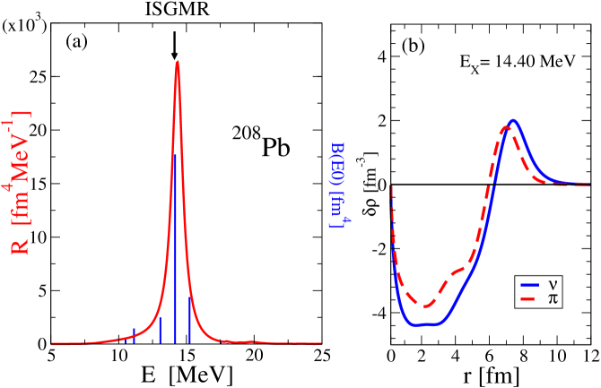
Figure 1: (Color online) (a) The isoscalar monopole spectrum in ²⁰⁸Pb, calculated with the parameter set PC-F1. The red curve corresponds to the strength distribution (units on the l.h.s.) obtained by a non-spectral representation without smearing ($\Delta=0$), the blue lines give the discrete B(E0)-values (units on the r.h.s.) obtained by the spectral representation with the same force. The black arrow indicates the experimental centroid energy of the resonance [37]. (b) the neutron and proton transition densities at the peak with the energy $E=14.40$ MeV.

Using the CRPA approach, we find for the calculated centroid energy defined in Eq. (70) that $m_{1}/m_{0}=14.40\,$ MeV, which is rather close to the result $m_{1}/m_{0}=14.17$ MeV deduced from discrete RPA calculations as well as to the experimental value $m_{1}/m_{0}=13.96\pm 0.2$ MeV [37].

In those two methods, no additional smearing $\Delta=0$ has been used. This means that the observed width of the continuum RPA strength corresponds entirely to the escape width which in the Pb region is very small, due to the relatively high Coulomb and centrifugal barriers in this heavy nucleus. In contrast, discrete RPA provides no width at all. Otherwise, the agreement of these two methods in this nucleus is excellent.

In the panel (b) of Fig. 1, we give the neutron and proton transition densities at the peak energy, as it is calculated in Eq. (72). They emphasize the collective character of the isoscalar breathing mode extended over the entire interior of the nucleus with neutrons and protons always in phase.

In addition, the energy weighted sum rule obtained in CRPA using Eq. (69) is $m_{1}(E0)=5.448\cdot 10^{5}$ [MeV$\cdot$fm⁴]. This result is in excellent agreement with the DRPA calculation $m_{1}(E0)=5.446\cdot 10^{5}$ [MeV$\cdot$fm⁴] as well as the classical value $m_{1}(E0)=4A\hbar/2m\langle r^{2}\rangle=5.453\cdot 10^{5}$ [MeV$\cdot$fm⁴]. This shows that the results obtained in the literature by relativistic RPA calculations using the spectral method are very reliable for such heavy nuclei [17, 8].

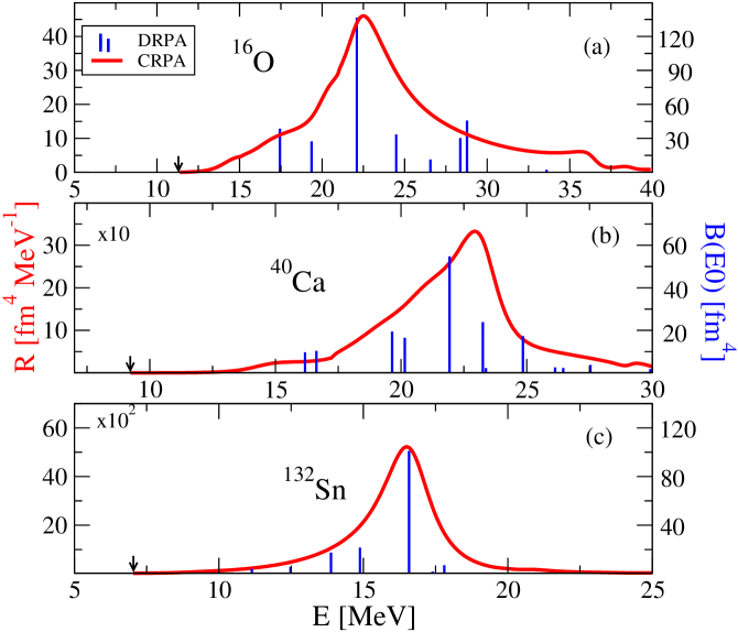
Figure 2: (Color online) The isoscalar monopole strength distribution for doubly magic nuclei (a) in ¹⁶O, (b) in ⁴⁰Ca, and (c) in ¹³²Sn. Details are the same as in the panel (a) of Fig. 1.

In Fig. 2 we show the E0 strength distributions for the lighter doubly magic nuclei ¹⁶O, ⁴⁰Ca, and ¹³²Sn. As in Fig. 1, the smearing parameter $\Delta$ is zero, but now the escape width is considerably larger for these nuclei. Fig. 3 summarizes the results for the isoscalar monopole strength distributions as a function of the mass number $A$. In panel (a), we plot the centroid energies of both continuum RPA (red dots) and discrete RPA (blue dots), together with the experimental centroid energies taken from Ref. [37]. We also show the phenomenological $A$-dependence $\bar{E}_{1^{-}}\approx 31.2\,A^{-1/3}+20.6\,A^{-1/6}$ by the dashed line. It becomes clear that CRPA can successfully reproduce collective excitations over the known range of nuclei.

Figure 3: (Color online) (a) The ISGMR centroid energies as a function of the mass number, (b) The experimental and theoretical width of the ISGMR as a function of the mass number. Details are given in the text.

In panel (b) of Fig. 3 we show the escape width $\Gamma^{\uparrow}$ of E0 resonances. The red values correspond to the full width half maximum (FWHM) of the peak, using continuum RPA , while the experimental values are indicated in black. The evident disagreement is not surprising, if we consider that only $1p1h$-configurations are taken into account, i.e. the major part of the width resulting from the coupling to more complicated configurations such as $2p2h$ etc. is not described well in this simple RPA approach. It has been shown in recent investigations of the coupling to complex configurations within the framework of the relativistic time-blocking approximation (RTBA) or the relativistic quasiparticle-time-blocking approximation (RQTBA) [24] that such couplings can be taken into account successfully in a fully consistent way starting from one density functional $E[\rho]$. So far, relativistic investigations of this type have been carried out with discrete methods. At present, investigations in this direction including the continuum properly go beyond the scope of this paper.

Isovector Giant Dipole Resonances

Isovector Giant Dipole resonance is the most well studied collective excitation and the first to be observed experimentally [38]. An external electromagnetic field of the form:

$$F_{L=1}^{T=1}=\frac{N}{A}\sum_{p=1}^{Z}r_{p}Y_{1M}(\Omega_{p})-\frac{Z}{A}\sum_{n=1}^{N}r_{n}Y_{1M}(\Omega_{n})$$ (75)

causes protons and neutrons to oscillate in opposite phases to each other and this leads to a pronounced peak in the photoabsorption cross section. This mode has been well studied in many nuclei [39].

With the increasing number of experiments in systems far from stability and systems with large neutron excess, one has been able to observe also low-lying E1 strength in the area of the neutron emission threshold. It is called Pygmy Dipole Resonance PDR and can be interpreted as a collective mode with dipole character where the neutron skin oscillates against an isospin saturated proton-neutron core. This mode has first been predicted in phenomenological models  [40] exhausting several percent of the electric dipole sum rule. In recent years, it has been intensively investigated both on the experimental side by the Darmstadt group [41, 42] as well as on the theoretical side, using discrete relativistic RPA calculations based on NL3 [43].

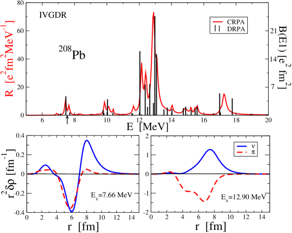
Figure 4: (Color online) (a) The isovector dipole strength distribution in ²⁰⁸Pb. Details are essentially the same as in the panel (a) of Fig. 1. However, in order to distinguish the continuum (red curve) and the discrete (blue lines) calculations we have used here a small smearing parameter $\Delta=10$ keV in the continuum calculation. The black arrow indicates the theoretical neutron emission threshold. (b) transition densities for neutrons and (c) for protons at the energy of the PDR (left) and at the GDR (right).

In Fig. 4 we show in panel (a) the results of the isovector dipole strength E1 in the nucleus ²⁰⁸Pb using the CRPA approach. The centroid energy at $13.32$ MeV is in excellent agreement with the experimental excitation energy $E=13.3$ MeV [44]. The energy weighted sum rule (69) is found as $m_{1}(E1)=916.28$ [MeV$\cdot$fm²]. This result is in agreement with the DRPA calculation, where we obtain $m_{1}(E1)=943.32$ [MeV$\cdot$fm²] and as usual somewhat (23.8 %) larger than the classical Thomas-Reiche-Kuhn sum rule

$$m_{\rm TRK}=\frac{9}{4\pi}\frac{\hbar^{2}}{2m}\frac{NZ}{A}=740.13~{}[{\rm MeV}\cdot{\rm fm}^{2}].$$ (76)

In addition to the giant dipole resonance a smaller peak appears at the energy region of the neutron emission threshold around $E\sim 7.5$ MeV, that corresponds to the pygmy resonance.

In panel (b) of Fig. 4 we give the transition densities associated the low-lying peak at $E=7.66$ MeV and the GDR peak at $E=12.9$ MeV. The higher peak has clearly an isovector character, since the neutrons are oscillating against the protons over a large radial range centered at the surface. The lower peak shows an isoscalar core, where neutrons and protons oscillate in phase and a pure neutron skin moving against the $T=0$ core. This is the typical behavior of the pygmy mode.

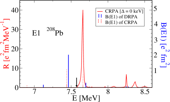
Figure 5: (Color online) The E1 pygmy resonance (PDR) in the nucleus ²⁰⁸Pb. The black arrow indicates the theoretical neutron emission threshold at $7.58$ MeV. The red dashed lines are obtained by CRPA calculations below the threshold.

	CRPA				DRPA
No.	E		B(E1)		E		B(E1)
1	6.	90	0.	19	7.	12	0.	23
2	7.	44	1.	45	7.	46	2.	82
3	7.	66	1.	11	7.	69	0.	40
$\Sigma$			2.	75			3.	45

Table 2: Energies and B(E1) values for the three most dominant peaks in the PDR area around the neutron threshold for the nucleus ²⁰⁸Pb for continuum (CRPA) and discrete (DRPA) calculations.

Closer investigation of pygmy resonances have shown that this mode is in the neighborhood of the neutron separation threshold, slightly below for small and slightly above for large neutron excess (see for instance Ref. [20]). It is therefore of particular importance to study this mode with a proper treatment of the continuum, since in most of the previous investigations this has not been possible. We show in Fig. 5 the details of the PDR in the nucleus ²⁰⁸Pb. Above the theoretical neutron separation threshold which is found at $E_{\mathrm{th}}=7.58$ MeV (black arrow) we have a continuous red curve showing the E1 strength distribution calculated with CRPA (units at the l.h.s) and also few full blue vertical lines that correspond to the discrete poles of the DRPA equations (63) (units at the r.h.s.) and with length equal to the corresponding B(E1) values.

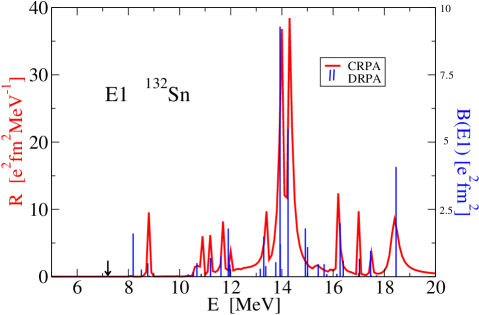
Figure 6: (Color online) The isovector dipole strength distribution in ¹³²Sn. Details are the same as in panel (a) of Fig. 4.

In the same figure and below the threshold we have in both cases discrete lines. The solid blue ones are again the eigen-solutions of the DRPA-equation (46). The solutions of the CRPA equations lead in this region also to discrete poles. We show them by dashed red lines at the pole of the full response function. Numerically, the only way to determine the B(E1) values of these poles in CRPA is by using very small imaginary parts $\Delta\rightarrow 0$ in the frequency $\omega+i\frac{1}{2}\Delta$ and then determining the B(E1) values by simple integration over a small interval around this pole.

By doing that, we finally observe that there are differences in the details between the continuum and the discrete RPA calculations close to the neutron separation threshold. In Table 2 we show for both calculations the three most dominant peaks in the area of the PDR around $7.5$ MeV. In the discrete calculations (DRPA) the strength is concentrated in one peak at $E=7.46$ MeV, whereas in the continuum calculations (CRPA) most of the strength in this region is distributed over two peaks, one below the neutron threshold at $E=7.44$ MeV and a sharp resonance slightly above the threshold at $E=7.66$ MeV. The energy weighted strength in this area is 17.09 [e²fm²] (i.e. 1.86 % of the total sum rule) for CRPA and 26.95 [e²fm²] (i.e. 2.85 % of the total sum rule) for DRPA.

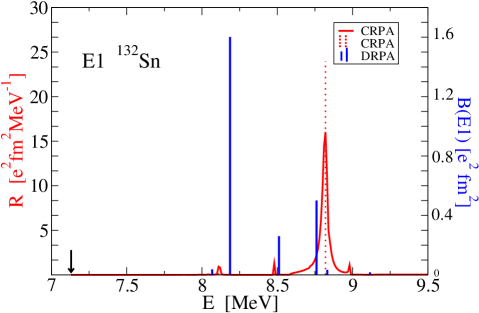
Figure 7: (Color online) The E1 pygmy resonance (PDR) in the nucleus ¹³²Sn. Details are the same as in Fig. 5. The arrow indicates the theoretical neutron emission threshold at $E_{\mathrm{th}}=7.13$ MeV.

In Fig. 6 we show the distribution of the isovector dipole strength in the doubly magic nucleus ¹³²Sn. Again, results using continuum RPA equations (red curve) are compared with the solutions obtained from the spectral representation (blue lines). As one can see, there is excellent agreement between the two methods, as far as the resonance position and the overall distribution is concerned. Moreover, the energy weighted sum rule obtained in CRPA is given by $m_{1}(E1)=563.60$ [MeV$\cdot$fm²], which is in very good agreement with the DRPA calculation $m_{1}(E1)=591.02$ [MeV$\cdot$fm⁴] and 22,9 % larger than the Thomas-Reiche-Kuhn sum rule in Eq. (76)

	CRPA				DRPA
No.	E		B(E1)		E		B(E1)
1	8.	11	0.	03	8.	067	0.	037
2	8.	48	0.	02	8.	186	1.	601
3	8.	82	1.	44	8.	511	0.	260
$\Sigma$			1.	490			1.	898

Table 3: Energies and B(E1) values for the three most dominant peaks in the PDR area above the neutron threshold for the nucleus ¹³²Sn for continuum (CRPA) and discrete (DRPA) calculations. The units are MeV for the energies and [e²fm²] for the B(E1) values. More details are given in the text

In addition, we find that the escape width in this nucleus is considerably smaller in the E1 channel as compared to the E0 channel in Fig. 2. This has the following explanation: The selection rules for $ph$-excitations with E0 character is $\Delta j=0$ and no change in parity. It turns out that most of the $ph$-excitations contributing to the strong peak in the resonance region have rather small $\ell$ values for the particle configurations and therefore a very low or no centrifugal barrier. This is different for the E1 resonance, where one has a change in parity and in addition changes of $\Delta j=0,\pm 1$. In such a case, a large part of the contributing $ph$-pairs have particles with larger $\ell$-values i.e. a strong centrifugal barrier and hence the width becomes smaller.

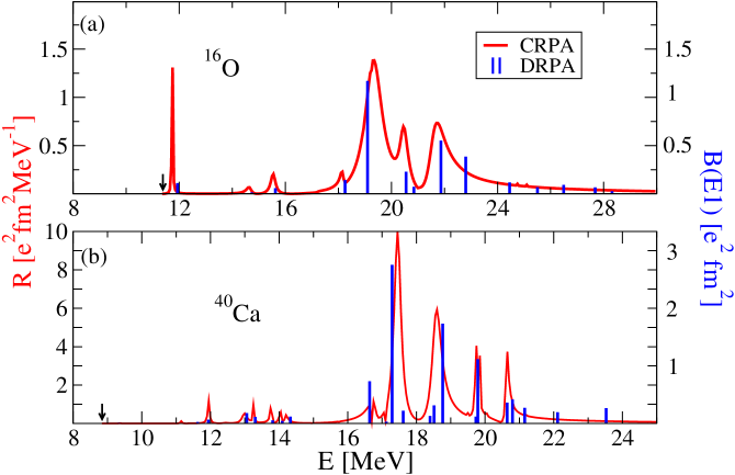
Figure 8: (Color online) The isovector dipole strength distribution in the nuclei ¹⁶O (a) and ⁴⁰Ca (b). Details are the same as in panel (a) of Fig. 4. The theoretical neutron separation energies, indicated by black arrow are $E_{\mathrm{thr}}=11.33$ MeV for ¹⁶O and $E_{\mathrm{thr}}=8.91$ MeV for ⁴⁰Ca.

In Fig. 7 we show the region of the PDR in the doubly magic nucleus ¹³²Sn. As already found in Ref. [20], the theoretical neutron emission threshold at $E=7.13$ MeV lies much below the area of interest. As before, we calculate the B(E1) values of the prominent peaks, for both discrete and continuum calculations with the total strength to be in good agreement. In Table 3 we show in what extent each level contributes to the total pygmy collective state. Finally, the energy weighted strength $m_{1}$ in this area is 13.24 [e²fm²] (i.e. 2.35 % of the total sum rule) for CRPA and 20.45 [e²fm²] (i.e. 3.46 % of the total sum rule) for DRPA.

In Fig. 8 we show the electric dipole strength distribution of the lighter nuclei ¹⁶O and ⁴⁰Ca. The strength obtained in CRPA calculations (red curves) are compared with the B(E1)-values resulting from discrete DRPA calculations (blue lines). The position of the corresponding peaks and poles with large strength are in rather good agreement, as explained in Table 4. We find, however, that in the continuum calculations a much larger escape width emerges, in particular for the nucleus ¹⁶O.

	CRPA	DRPA	Exp.
16O	20.6279	21.623	23.35$\pm$0.12 [45]
40Ca	18.367	19.32	21.76$\pm$0.11 [46]
132Sn	14.503	14.78
208Pb	13.32	13.23	13.3$\pm$0.10 [44]

Table 4: Isovector dipole ($IVGDR$) excitation energies in [MeV] for several spherical nuclei, calculated with both continuum and discrete relativistic $RPA$ based on the point coupling force PC-F1.

Isoscalar Giant Dipole Resonances

Besides the distribution of the isovector dipole strength which is dominated by the IVGDR in many experimental spectra, in recent years there has also been considerable interest in measuring the isoscalar dipole strength distribution [47, 48]. In a similar way, one expects to find the ISGDR, which corresponds to a compression wave going through the nucleus along a definite direction and to learn from such experiments more about the nuclear incompressibility. Relativistic calculations based on discrete RPA [17, 23] have shown that the resonance energy of this mode is indeed closely connected to the incompressibility of nuclear matter.

Along with this ISGDR resonance built on $3\hbar\omega$-excitations above 20 MeV, calculations based on both relativistic [17] and non-relativistic [49] RPA approaches have revealed a low-lying isoscalar dipole strength in the region below and around 10 MeV. Experimental investigations with inelastic scattering of $\alpha$-particles at small angles [50, 48] have also found isoscalar dipole strength in this region. This strength has been attributed in Ref. [19] to an exotic mode of a toroidal motion predicted already in early theoretical investigations on multipole expansions of systems with currents [51] and investigated also by semiclassical methods [52]

On the theoretical point of view, there is further interest in the isoscalar dipole mode, characterized by the quantum numbers ($J^{\pi}=1^{-},T=0$), because it contains the Goldstone mode connected with the violation of translational symmetry in the mean field solutions. This mode corresponds to the center of mass motion of the entire nucleus. Because of the missing restoring force, this mode has vanishing excitation energy. It is one of the essential advantages of the RPA approximation, that it preserves translational symmetry and therefore it has an eigenvalue at zero energy with the eigenfunction given by the $ph$-matrix elements of the linear momentum operator.

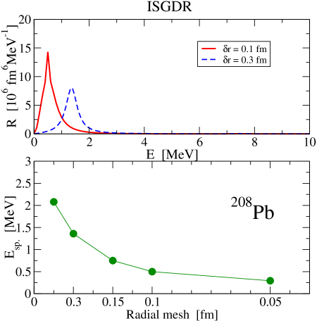
Figure 9: (Color online) (a) Spurious E1 isovector strength distribution in ²⁰⁸Pb obtained by CRPA calculations with two different values of the radial mesh size $\delta r$. (b) the position of the spurious E1-state as a function of the radial mesh size

Since the ISGDR is expected to be a $3\hbar\omega$-excitation it is usually associated with the external field derived in Ref. [54]

$$F_{L=1}^{T=0}~{}=~{}\sum_{i}^{A}(r_{i}^{3}-\eta r_{i})Y_{1\mu}(\Omega_{i}),$$ (77)

where the factor $\eta=\frac{5}{3}\langle r^{2}\rangle$ is used to extract the spurious center of mass motion.

In the upper part of Fig. 9 we display the distribution of the isoscalar dipole strength in ²⁰⁸Pb, calculated with the operator (77) for $\eta=0$, that is, we take no action for the spurious state. We therefore observe a huge peak close to zero energy, which dominates the spectrum and corresponds to the spurious translational mode.

It turns out that the position of this spurious state is an extremely sensitive object which strongly depends on the numerics of the model. Of course the optimal would be to calculate the spurious state at exactly zero energy. Therefore this excitation mode presents an ideal benchmark for numerical efficiency of the RPA or the linear response equations. Detailed studies have shown that the exact separation of the spurious state requires a fully self-consistent solution [22]; a fact which was not given in most of the older applications with Skyrme or Gogny forces. In many cases, only few of the different terms in the residual interaction had been taken into account in RPA calculations.

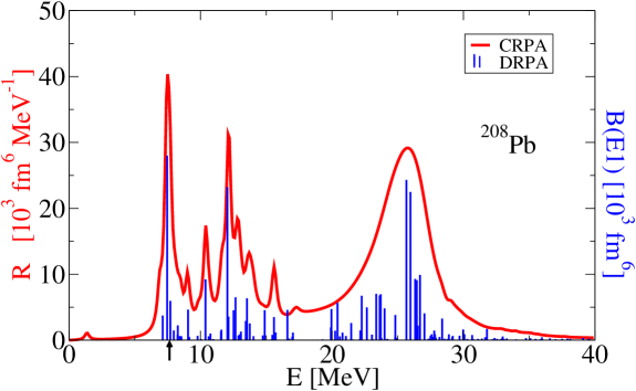
Figure 10: (Color online) The isoscalar dipole strength distribution in ²⁰⁸Pb. Details are the same as in the panel (a) of Fig. 4.

In addition, the configuration space must be full. Indeed, the discussed drawback of the conventional spectral representation in a truncated $ph$-configuration space affects the position of the spurious state. Therefore, the convergence to zero eigenvalue of the spurious translational mode occurs very slowly and only in extremely large configuration space. In relativistic applications this is translated to including also large spectrum in the Dirac sea [15, 8]. As a consequence, in the spectral representation, one has to take into account many configuration with particles in the Dirac and holes in the Fermi sea, which complicates the numerical applications considerably and inevitably decreases the efficiency of the method.

Fortunately, using the continuum RPA approach, one is free from such constraints and limitations, since the entire configuration space is automatically included. The results in Fig. 9 obtained with the operator (77) for $\eta=0$ show clearly the spurious state dominating the entire spectrum (see the scale). Its position is not precisely at zero energy, rather it depends on the mesh size used for the solution of the continuum response equation (the response mesh). In panel (a) of Fig. 9 we present two calculations with different mesh-sizes, where in panel (b) we show how the spurious state moves to zero energy as we use a finer radial interval. For the ideal case of an infinitesimal mesh, the strength connected with the spurious state would be completely separated from the rest of the spectrum.

In Fig. 10 we show results obtained with the full operator (77), i.e. with $\eta=\frac{5}{3}\langle r^{2}\rangle$, in a scale increased by three orders of magnitude. Obviously this procedure removes the spurious state with high precision. We also did not observe any influence of the isoscalar mode in the isovector channel due to isospin mixing. In this context we have to remember, that the isospin mixing introduced on the mean field level is corrected on the RPA level to a large extend [12].

The main part of the remaining isoscalar dipole spectrum in Fig. 10 is located at $E\approx 25$ MeV. This ”exotic” mode is best described as a ”hydrodynamical density oscillation”, in which the volume of the nucleus remains constant and the state can be visualized as a compression wave oscillating back and forth through the nucleus [19].

	Low[MeV]		High[MeV]
CRPA	10.	97	25.	05
Hamamoto et al [55]	$\sim$ 14		23.	4
Coló et al [56]	10.	9	23.	9
Vretenar et al. [17]	10.	4	26.
Piekarewicz [23]	$\sim$  8		24.	4
Shlomo, Sanzhur [57]	$\sim$ 15		$\sim$ 25
Uchida et al. [48]	12.	7 $\pm$ 0.2	22.	4 $\pm$ 0.5

Table 5: Self-consistent (relativistic and non-relativistic) RPA calculations performed for the ISGDR in ²⁰⁸Pb, compared with the most recent experimental data. The two columns refer to the centroid energies of both the low- and high-energy sides of the ISGDR mode.

Moreover, Fig. 10 shows an additional mode in the region of $10-15$ MeV that exhausts roughly $20\%$ of the total sum rule. This peak does not correspond to a compression mode, but as discussed in Ref. [19] rather to a kind of toroidal motion. The toroidal dipole mode is understood as a transverse zero-sound wave and its experimental observation would invalidate the hydrodynamical picture of the nuclear medium, since there is no restoring force for such modes in an ideal fluid.

In conclusion, continuum RPA calculations manage not only to predict the existence of the toroidal and the compression mode, but also to achieve a reasonable agreement of the corresponding centroid energies to other models focusing on the same problem, as well as to recent experimental data [48, 47]. In Table 5, these results are presented for the case of the well studied nucleus ²⁰⁸Pb.

6 Conclusions

Starting from a point coupling Lagrangian, we have used the non-spectral relativistic RPA approach to examine the corresponding excitation spectra and we have compared the results with spectral calculations based on the same Lagrangian. This non-spectral method has several advantages. The coupling to the continuum is treated consistently using the relativistic single particle Green’s function at the appropriate energy. In this way, complicated sums over unoccupied states are avoided. This is particularly important for relativistic applications since the Dirac sea is now automatically treated properly and the unphysical transitions from holes in the Fermi sea to particles in the Dirac sea is avoided as long as we restrict our investigations to positive energies.

The ground state phenomena are calculated using the same Lagrangian by a self-consistent solution of the relativistic mean field equations in $r$-space. The residual particle-hole interaction used in the RPA calculations is derived in a fully self-consistent way from the second derivative of the corresponding energy density functional. In this way no additional parameters are required and one is able to reproduce the collective properties, namely the multipole giant resonances for various doubly closed shell spherical nuclei over the entire periodic table.

The calculations are carried out by using a new relativistic continuum RPA program for point-coupling models, that includes all the terms in the Lagrangian, in particular the two-body interactions with zero range, the density dependent parts with all the rearrangement terms, the derivative terms, the various current-current terms and the Coulomb interaction. As applications the nuclei ¹⁶O, ⁴⁰Ca, ⁹⁰Zr, ¹³²Sn, and ²⁰⁸Pb have been investigated proving that a hight level of accuracy is achieved, as compared to the discrete methods. Comparing calculations with spectral and non-spectral representations of the response function for the same Lagrangian we find, that in general the spectra are well reproduced within the spectral approximation, if an appropriate phenomenological smearing parameter is used and if a sufficiently large number of $ph$-configurations is taken into account in the latter case. We find, however, differences in neighborhood of the neutron threshold, where the coupling to the continuum is not properly reproduced in the spectral method.

As compared to the discrete case the non-spectral representation has the advantage of (i) a precise treatment of the coupling to the continuum and a fully consistent determination of the escape width without a phenomenological smearing parameter, (ii) a faster evaluation of the cross section, because one needs for fixed energy only two scattering solutions instead of the thousands of $ph$-configurations in the discrete case and (iii) a proper treatment of the Dirac sea without any further $ah$-configurations.

Relativistic CRPA describes very well the position of resonances in doubly magic spherical nuclei. Provided that proper pairing correlations are taken into account, a similar method can also be applied in open-shell nuclei. This requires the development of the relativistic continuum quasiparticle random phase approximation (CQRPA). This approach accounts on equal footing for the influence of the residual particle-hole ($ph$) as well as the particle-particle ($pp$) correlations. In analogy to non-relativistic calculations [58, 59, 60, 61] this can be achieved on the basis of relativistic CRPA theory developed in this manuscript either by treating the pairing correlations in the BCS approach for nuclei far from the drip lines where no level in the continuum is occupied, or in the Hartree-Bogoliubov approximation valid for all nuclei up to the drip line. Investigations in this direction are in progress.

Of course, the present approach is based on the RPA and includes only $1p1h$-configurations. Therefore only the escape width of the resonances can be reproduced properly. For heavy nuclei the decay width resulting from a coupling to more complex configurations is very important. In fact, such couplings have been introduced successfully in the relativistic scheme using the spectral representation in Refs. [24]. On the non-relativistic side, such techniques have also been used in the context of the non-spectral representation without [62, 63] and with [64] pairing. So far, however, fully self-consistent relativistic applications including complex configurations with a proper treatment of the continuum are still missing.

Helpful discussions with G. Lalazissis, E. Litvinova, T. Nikšić, N. Paar, V. Tselyaev, and D. Vretenar are gratefully acknowledged. This research has been supported the Gesellschaft für Schwerionenforschung (GSI), Darmstadt, the Bundesministerium für Bildung und Forschung, Germany under project 06 MT 246 and by the DFG cluster of excellence “Origin and Structure of the Universe” (www.universe-cluster.de).

Appendix A The effective interaction in density dependent point-coupling models

In Eq. (40) the effective interaction for RPA calculations is defined as the second derivative of the energy functional with respect to the density matrix:

$$V_{\alpha\beta\alpha^{\prime}\beta^{\prime}}^{\text{ph}}=\frac{\delta^{2}E[\hat{\rho}]}{\delta\hat{\rho}_{\alpha\beta}\delta\hat{\rho}_{\alpha^{\prime}\beta^{\prime}}}.$$ (78)

In coordinate representation the indices $\alpha$,$\beta,\dots$ are an abbreviation for the ”coordinates” $1=({\bm{r}_{1}},s_{1},d_{1},t_{1})$, where $s$ is the spin and $t$ the isospin coordinate, and $d=1,2$ is the Dirac-index for large and small components. Starting from the energy density functional (7) and neglecting for the moment the Coulomb force, we find the density dependent zero range force

$$V^{\text{ph}}(1,2)~{}=~{}\sum\limits_{c}\Gamma_{c}^{(1)}~{}\delta({\bm{r}}_{1}-{\bm{r}}_{2})\upsilon_{c}({\bm{r}}_{1})\Gamma_{c}^{{\dagger}(2)}$$ (79)

where the vertices $\Gamma_{c}$ are 8$\times$8 matrices acting on the indices $s,d,t$ and reflect the different covariant structures of the fields including spin and isospin degrees of freedom. We express the 4$\times 4$ Dirac matrices as a direct product of spin matrices $\sigma$ and 2$\times 2$ matrices $\gamma_{D}$ acting on large and small components

$$\gamma_{0}=\left(\begin{array}[c]{cc}1&0\\ 0&-1\end{array}\right),~{}~{}~{}1=\left(\begin{array}[c]{cc}1&0\\ 0&1\end{array}\right),~{}~{}~{}\gamma_{5}=\left(\begin{array}[c]{cc}0&1\\ 1&0\end{array}\right)$$ (80)

and the spin matrices $\sigma_{S=0}=1$ and $\sigma_{S=1}=\sigma_{\mu}$ with the spherical coordinates of the Pauli spin matrices. In this way we obtain the vertices $\Gamma_{c}=\gamma_{D}\times\sigma_{S}\times\tau_{T}$ as direct products of 2-dimensional Dirac-, spin- and isospin matrices (see also the second column of Table 6).

Finally, in Eq. (79) the quantities $\upsilon_{c}({\bm{r}})$ describe the strengths of all the various parts of the interaction derived in a consistent way from the Lagrangian. The ones derived from the four-fermion terms (3) are constants. Furthermore, due to a density dependence of the higher order terms (4) as well as the corresponding rearrangement terms, $\upsilon_{c}({\bm{r}})$ depends on the static density and therefore on the coordinate ${\bm{r}}$. In addition, because of the derivative terms (5), they also contain Laplace operators. Summarizing, we have:

$$\begin{array}[c]{ll}\text{ \ \ \ }c&\text{ \ \ }\upsilon_{c}(r)=\\ \text{scalar:}&\text{ \ \ }\alpha_{S}+2\beta_{S}\rho_{S}({r})+3\gamma_{S}\rho_{S}^{2}({r})+\delta_{S}\Delta\\ \text{time-like vector:}&\text{ \ \ }\alpha_{V}+3\gamma_{V}\rho_{V}^{2}({r})+\delta_{V}\Delta\text{ \ \ \ \ \ \ \ \ \ \ \ \ \ \ \ \ \ }\\ \text{space-like vector:}&\text{ \ }-\alpha_{V}-\gamma_{V}\rho_{V}^{2}({r})-\delta_{V}\Delta\end{array}$$ (81)

In the isovector case the constants $\alpha_{S}$, $\alpha_{V}$, $\delta_{S}$ and $\delta_{V}$ are replaced by $\alpha_{TS}$, $\alpha_{TV}$, $\delta_{TS}$ and $\delta_{TV}$. As we see in Table 1 the corresponding values $\beta_{TS}=$ $\gamma_{TS}=\gamma_{TV}$ vanish.

For spherical nuclei, the densities and currents in the Lagrangian depend only on the radial coordinate $r$. Therefore we expand the $\delta$-function in Eq. (79) in terms of spherical harmonics

$$\delta({\bm{r}}_{1}-{\bm{r}}_{2})~{}=~{}\frac{\delta(r_{1}-r_{2})}{r_{1}r_{2}}\sum_{L}Y_{L}(\Omega_{1})\cdot Y_{L}(\Omega_{2}).$$ (82)

Combining spin ($S$) and orbital ($L$) degrees of freedom we find by re-coupling to total angular momentum $J$

$$(\mathbf{\sigma}^{(1)}_{S}\cdot\mathbf{\sigma}^{(2)}_{S})(Y_{L}(1)\cdot Y_{L}(2))=\sum_{J}[\mathbf{\sigma}_{S}Y_{L}]_{J}^{(1)}\cdot[\mathbf{\sigma}_{S}Y_{L}]_{J}^{(2)}$$ (83)

Inserting this expression into Eq. (81) we obtain for the interaction a sum (or integral) of separable terms (channels)

$$V^{\text{ph}}(1,2)~{}=~{}\sum\limits_{c}\int\limits_{0}^{\infty}dr~{}Q_{c}^{(1)}(r)~{}\upsilon_{c}(r)~{}Q_{c}^{{\dagger}(2)}(r)$$ (84)

Each channel is characterized by a continuous parameter $r$ and the discrete numbers $c=(D,S,L,J,T)$. The corresponding channel operators $Q_{c}^{(1)}(r)$ are local single particle operators

$$Q_{c}^{(1)}(r)~{}=~{}\frac{\delta(r-r_{1})}{rr_{1}}\gamma^{(1)}_{D}\left[\sigma^{(1)}_{S}Y_{L}(\Omega_{1})\right]_{J}\tau^{(1)}_{T}$$ (85)

and the upper indices (1) and (2) in Eq. (84) indicate that these operators act on the ”coordinates” $1=(r_{1}\Omega_{1}s_{1}d_{1}t_{1})$ and $2=(r_{2}\Omega_{2}s_{2}d_{2}t_{2})$.

The total angular momentum is a good quantum number and for fixed $J$ the sum over $c$ in Eq. 84 runs only over specific numbers $c=(D,S,L,T)$ determined by the selection rules. We concentrate in this manuscript on states with natural parity, i.e. $\pi=(-)^{L}=(-)^{J}$. Considering that $S=0$ for the scalar and the time-like vector and that $S=1$ for the space-like vector we therefore have

$$L=\left\{\begin{array}[]{cc}J&\text{for $S=0$}\\ J\pm 1&\text{for $S=1$}\end{array}\right.$$

Finally we have eight discrete channels. Their quantum numbers are shown in Table 6.

c	$\Gamma_{c}=\gamma_{D}$$\,\otimes\,$	$\sigma_{S}$ $\,\otimes\,$	$\tau_{T}$	$D$	$S$	$L$	$T$
1	$\gamma_{0}$$\,\otimes\,$	1 $\,\otimes\,$	1	$S$	0	$J$	0
2	1$\,\otimes\,$	1 $\,\otimes\,$	1	$V$	0	$J$	0
3	$\gamma_{5}$$\,\otimes\,$	$\sigma$ $\,\otimes\,$	1	$V$	1	$J-1$	0
4	$\gamma_{5}$$\,\otimes\,$	$\sigma$ $\,\otimes\,$	1	$V$	1	$J+1$	0
5	$\gamma_{0}$$\,\otimes\,$	1 $\,\otimes\,$	$\tau_{3}$	$S$	0	$J$	1
6	1$\,\otimes\,$	1 $\,\otimes\,$	$\tau_{3}$	$V$	0	$J$	1
7	$\gamma_{5}$$\,\otimes\,$	$\sigma$ $\,\otimes\,$	$\tau_{3}$	$V$	1	$J-1$	1
8	$\gamma_{5}$$\,\otimes\,$	$\sigma$ $\,\otimes\,$	$\tau_{3}$	$V$	1	$J+1$	1

Table 6: Vertices and quantum numbers of the different channels in Eq. (79)

An essential feature of the effective interaction $(\ref{VphC})$ is that it contains derivative terms in the form of Laplacians $\Delta$ (retardation effects are neglected). In spherical coordinates, they contain radial derivatives as well as angular derivatives. The latter can be expressed by the angular momentum operators acting on spherical harmonics $Y_{LM}$. Therefore we obtain:

$$\Delta=r^{2}\overleftarrow{\partial}_{r}\frac{1}{r^{2}}\overrightarrow{\partial}_{r}+\frac{L(L+1)-2}{r^{2}}.$$ (86)

Here the radial derivatives $\overleftarrow{\partial}_{r}$ and $\overrightarrow{\partial}_{r}$ act on the right and on the left side in Eq. (67), i.e. on $\mathcal{R}_{c^{\prime}c}^{\,0}(r^{\prime}r)$ and on $\mathcal{R}_{cc^{\prime\prime}}(r,r^{\prime\prime})$. Since the integration is discretized $r\rightarrow r_{n}=$ $nh$ the operator $\overrightarrow{\partial}_{r}$ is represented by a matrix in $r$-space as for instance by the tree-point formula:

$$\hat{\partial}_{nn^{\prime}}=\frac{1}{2h}(\delta_{n^{\prime},n+1}-\delta_{n^{\prime},n-1}).$$ (87)

This means that the term $\upsilon_{c}(r)$ in Eq. (4) is no more diagonal in the coordinate $r$ and it must be replaced by a matrix $\upsilon_{c}(r,r^{\prime})$.

The term which leads to off-diagonal terms in channel space is the Coulomb interaction. It brakes isospin symmetry and therefore it will be described by the general form $\upsilon_{cc^{\prime}}(r,r^{\prime})$. In particular, we will have

$$V_{\text{C}}(1,2)=(\frac{1}{2}(1-\tau_{3}))^{(1)}\frac{\alpha}{|\mathbf{r}_{1}\mathbf{-r}_{2}|}(\frac{1}{2}(1-\tau_{3}))^{(2)}$$ (88)

and the $r$ dependance can be written as:

$$\frac{\alpha}{|\mathbf{r}_{1}\mathbf{-r}_{2}|}=\sum\limits_{L}\upsilon_{\text{C}}(r,r^{\prime})Y_{L}(\Omega)\cdot Y_{L}(\Omega^{\prime})$$ (89)

with

$$\upsilon_{\text{C}}(r,r^{\prime})=\frac{4\pi\alpha}{2L+1}\cdot\frac{r_{<}^{L}}{r_{>}^{L+1}},$$ (90)

and $r_{<}$ and $r_{>}$ are the smaller and the greater of $r$ and $r^{\prime}$. This leads to a matrix $\upsilon_{cc^{\prime}}(r,r^{\prime})$ in Eq. (4) as shown in Table 7.

	$\beta$	$1$	$\alpha$	$\beta\vec{\tau}$	$\vec{\tau}$	$\mbox{\boldmath$\alpha$}\vec{\tau}$
$\beta$	0	0	0	0	0	0
1	0	$+\frac{1}{4}\upsilon_{C}$	0	0	$-\frac{1}{4}\upsilon_{C}$	0
$\alpha$	0	0	- $\frac{1}{4}\upsilon_{C}$	0	0	$-\frac{1}{4}\upsilon_{C}$
$\beta\vec{\tau}$	0	0	0	0	0	0
$\vec{\tau}$	0	$-\frac{1}{4}\upsilon_{C}$	0	0	$+\frac{1}{4}\upsilon_{C}$	0
$\mbox{\boldmath$\alpha$}\vec{\tau}$	0	0	$-\frac{1}{4}\upsilon_{C}$	0	0	$-\frac{1}{4}\upsilon_{C}$

Table 7: The structure of the channel matrix $\upsilon_{cc^{\prime}}(r,r^{\prime}$) for the Coulomb interaction.

Appendix B The continuum representation for the Green’s function

In a non-spectral or continuum approach the relativistic single particle Green’s function $G_{\kappa}(r,r^{\prime};E)$ obeys the equation:

$$\left(E-\hat{h}_{\kappa}(r)\right)G_{\kappa}(r,r^{\prime};E)=\delta(r-r^{\prime}),$$ (91)

where $\hat{h}_{\kappa}(r)$ is the radial Dirac-operator of Eq. (33) depending on the quantum number $\kappa=(lj)$. This Green’s function can be constructed at each energy $E$ from two linearly independent solutions

$$|u(r)\rangle = {\binom{f_{u}(r)}{g_{u}(r)}},\qquad|w(r)\rangle={\binom{f_{w}(r)}{g_{w}(r)}}$$ (92)

$$\langle u^{*}(r)| = (f_{u}(r)\,g_{u}(r)),\langle w^{*}(r)|=(f_{w}(r)\,g_{w}(r))$$ (93)

of the Dirac equation with the same energy $E$

$$\left(E-\hat{h}_{\kappa}(r)\right)|u(r)\rangle=0,\text{ \ \ \ \ }\left(E-\hat{h}_{\kappa}(r)\right)|w(r)\rangle=0,$$ (94)

but with different boundary conditions. The functions $\ u(r)$ and $w(r)$ are normalized in such a way that the Wronskian is equal to:

$$W=\left|\begin{array}[c]{cc}f_{w}(r)&f_{u}(r)\\ g_{w}(r)&g_{u}(r)\end{array}\right|=f_{w}(r)g_{u}(r)-g_{w}(r)f_{u}(r)=1.$$ (95)

Of course these scattering solutions depend on the energy $E$ and on the quantum number $\kappa$, i.e. we have $|u_{\kappa}(r,E)\rangle$ and $|w_{\kappa}(r,E)\rangle$. The Dirac-equation in $r$-space is a two-dimensional equation and therefore the corresponding single particle Green’s function is a 2$\times 2$ matrix. Using the bracket notation of Dirac for the 2-dimensional spinors and following Ref. [33] we can express this Green’s function as:

$$G_{\kappa}(r,r^{\prime};E)=\left\{\begin{array}[c]{cc}|w_{\kappa}(r;E)\rangle\langle u^{\ast}_{\kappa}(r^{\prime};E)|&\text{~{}~{}for}\,\,r>r^{\prime}\\ |u_{\kappa}(r;E)\rangle\langle w^{\ast}_{\kappa}(r^{\prime};E)|&\text{~{}~{}for}\,\,r<r^{\prime}\end{array}\right.$$ (96)

with

$$G_{\kappa}(r^{\prime},r;E)=G^{\top}_{\kappa}(r,r^{\prime};E)$$ (97)

The solution $u_{\kappa}(r)$ is regular at the origin, i.e. following Ref. [34] we have for $E>V+S$ in the limit $r\rightarrow 0$:

$$u(r)\rightarrow r{\binom{j_{l}(kr)}{\frac{\kappa}{|\kappa|}\frac{E-V-S}{k}j_{\tilde{l}}(kr)}\rightarrow\binom{\frac{r}{(2l+1)!!}(kr)^{l}}{\frac{\kappa}{|\kappa|}\frac{r(E-V-S)}{k(2\tilde{l}+1)!!}(kr)^{\tilde{l}}}},$$ (98)

with $k^{2}=(E-V-S)(E-V+S+2m)>0$ and $j_{l}(z)$ is a spherical Bessel function of the first kind. The wave function $w_{\kappa}(r)$ represents at large distances for $E>0$ an outgoing wave, i.e. we have for $r\rightarrow\infty$

$$w(r)\rightarrow{\binom{rh_{l}^{(1)}(kr)}{\frac{\kappa}{|\kappa|}\frac{ikr}{E+2m}h_{\tilde{l}}^{(1)}(kr)}\rightarrow\binom{1}{\frac{\kappa}{|\kappa|}\frac{ik}{E+2m}}}e^{ikr},$$ (99)

where $h_{l}^{(1)}(z)$ is the spherical Hankel function of the first kind and for $E<0$ an exponentially decaying state, i.e. we have for $r\rightarrow\infty$

$$w(r)\rightarrow{\binom{r\sqrt{\frac{2Kr}{\pi}}K_{l+\frac{1}{2}}(Kr)}{\frac{-Kr}{E+2m}\sqrt{\frac{2Kr}{\pi}}K_{\tilde{l}+\frac{1}{2}}(Kr)}\rightarrow\binom{1}{\frac{-K}{E+2m}}}e^{-Kr},$$ (100)

where $K^{2}=(V-S-E)(E-V+S+2m)>0$ and $j_{l}(z)$ and $K_{l+1/2}(z)$ are modified spherical Bessel functions [65]. For $E<0$ the two scattering solutions are both real. This absence of any imaginary term will eventually give no contribution to the cross section of Eq. (34). We have to keep in mind, however, that at energies that correspond to eigen energies of a bound state, the solutions $u_{\kappa}(r,E)$ and $w_{\kappa}(r,E)$ coincide up to a factor, which means that the Wronskian vanishes at this energy. This corresponds to a pole in the response function on the real energy axis. By adding a small imaginary part to the energy $E\rightarrow E+i\Delta$ we obtain a sharp peak in the strength distribution.

Appendix C The free response function in $r$-space

The reduced free response

$$R_{cc^{\prime}}^{0}(\omega)=\sum\limits_{ph}\frac{\langle h|Q_{c}^{+}|p\rangle\langle p|Q_{c^{\prime}}|h\rangle}{\omega-\varepsilon_{p}+\varepsilon_{h}}-\frac{\langle p|Q_{c}^{+}|h\rangle\langle h|Q_{c^{\prime}}|p\rangle}{\omega+\varepsilon_{p}-\varepsilon_{h}}$$ (101)

depends on the energy E and the channel indices $c,c^{\prime}$. The operators $Q_{c}$ given by Eq. (85) are characterized by the channel index $c=(r,DSLT)$. Each single particle matrix element of the form $\langle p|Q_{c}|h\rangle$ in Eq. (101) separates into an angular, an isospin and a radial part.

$$\langle p|Q_{c}|h\rangle=\langle p|\tau_{T}|h\rangle\langle\kappa_{p}||\left[\sigma_{S}Y_{L}\right]_{J}||\kappa_{h}\rangle\langle p|\gamma_{D}|h\rangle_{r}.$$ (102)

Since we consider in this paper only $ph$-RPA in the same nucleus, the particle states have the same isospin as the hole states and thus the isospin matrix element $\langle p|\tau_{T}|h\rangle$ is simply a phase $\pm 1$.

Considering that this channel operator has a $\delta$-function in the radial coordinate, the radial matrix elements $\langle p|\gamma_{c}|h\rangle_{r}=\langle p(r)|\gamma_{D}|h(r)\rangle$ then depend on $r$. They are found as sums over the large and small components in the radial spinors $|h(r)\rangle$ and $|p(r)\rangle$ for fixed values of $r$.

The angular matrix elements depend on the quantum numbers $\kappa$ of particle and hole states, and, of course, on the channel quantum numbers $S$ and $L$. In particular, we find for $S=0$:

$$\left\langle lj||Y_{J}||l^{\prime}j^{\prime}\right\rangle=\frac{1+(-)^{l+l^{\prime}+J}}{2}\frac{\hat{\jmath}\hat{\jmath}^{\prime}\hat{J}}{\sqrt{4\pi}}(-)^{j-\frac{1}{2}}\left(\begin{array}[c]{ccc}j&J&j^{\prime}\\ -\frac{1}{2}&0&\frac{1}{2}\end{array}\right)$$ (103)

while for $S=1$, it is

$$\langle lj||\left[\sigma Y_{L}\right]_{J}||l^{\prime}j^{\prime}\rangle = \frac{1+(-)^{l+l^{\prime}+L}}{2}\frac{\hat{\jmath}\hat{\jmath}^{\prime}\hat{L}\hat{J}}{\sqrt{4\pi}}\left[(-)^{j^{\prime}+\frac{1}{2}}\left(\begin{array}[c]{ccc}1&L&J\\ 0&0&0\end{array}\right)\left(\begin{array}[c]{ccc}j&J&j^{\prime}\\ \frac{1}{2}&0&-\frac{1}{2}\end{array}\right)\right.$$ (108)

$$- \left.\sqrt{2}(-)^{l^{\prime}}\left(\begin{array}[c]{ccc}1&L&J\\ -1&0&1\end{array}\right)\left(\begin{array}[c]{ccc}j&J&j^{\prime}\\ \frac{1}{2}&-1&\frac{1}{2}\end{array}\right)\right].$$ (113)

Using for the angular and isospin part the abbreviation

$$Q_{ph}^{c}=\langle\kappa_{p}||\left[\sigma_{S}Y_{L}\right]_{J}||\kappa_{h}\rangle\langle p|\tau_{T}|h\rangle,$$ (114)

we obtain for the reduced response function of Eq. (57) in $r$-space:

$$\mathcal{R}_{cc^{\prime}}^{0}(r,r^{\prime};\omega)=\sum\limits_{ph}\left\{Q_{ph}^{\ast c}Q_{ph}^{c^{\prime}}\frac{\langle h|\gamma_{c}^{+}|p\rangle_{r}\langle p|\gamma_{c^{\prime}}|h\rangle_{r^{\prime}}}{\omega-\varepsilon_{p}+\varepsilon_{h}}-Q_{hp}^{\ast c}Q_{hp}^{c^{\prime}}\frac{\langle h|\gamma_{c^{\prime}}|p\rangle_{r^{\prime}}\langle p|\gamma_{c}^{+}|h\rangle_{r}}{\omega+\varepsilon_{p}-\varepsilon_{h}}\right\}$$ (115)

As in Eq. (58) we extend the sum over $p$ over the full space and use completeness in the radial wave functions:

$$\mathcal{R}_{cc^{\prime}}^{\,0}(r,r^{\prime};\omega) = {\sum\limits_{h\kappa}}\left\{Q_{\kappa h}^{\ast c}Q_{\kappa h}^{c^{\prime}}\,\langle h(r)|\gamma_{c}^{+}G_{\kappa}(r,r^{\prime};\omega+\varepsilon_{h})\gamma_{c^{\prime}}|h(r^{\prime})\rangle\right.$$ (116)

$$+ \left.Q_{h\kappa}^{\ast c}Q_{h\kappa}^{c^{\prime}}\langle h(r^{\prime})|\gamma_{c}G_{\kappa}(r^{\prime},r;-\omega+\varepsilon_{h})\gamma_{c^{\prime}}^{+}|h(r)\rangle\right\}.$$

Since the angular matrix elements depend only on the quantum numbers $\kappa$ the sum over $p$ is here replaced by a sum over the quantum numbers $\kappa$, which is restricted by the selection rules of the reduced matrix elements (114). Having the exact form of the Green’s function for the static radial Dirac equation (33), one can finally construct the non-spectral or continuum reduced response function (4):

$$\mathcal{R}_{cc^{\prime}}^{\,0}(rr^{\prime};\omega) = \sum_{h\kappa}\left\{Q_{\kappa h}^{\ast c}Q_{\kappa h}^{c^{\prime}}\gamma_{hw}^{c}(r;\omega+\varepsilon_{h})\gamma_{uh}^{c^{\prime}}(r^{\prime};\omega+\varepsilon_{h})\right.$$

$$\qquad-\left.Q_{h\kappa}^{\ast c}Q_{h\kappa}^{c^{\prime}}\gamma_{hw}^{c}(r;\omega-\varepsilon_{h})\gamma_{uh}^{c^{\prime}}(r^{\prime};\omega-\varepsilon_{h})\right\}\mathrm{~{}~{}for~{}~{}}r>r^{\prime}$$

$$= \sum_{h\kappa}\left\{Q_{\kappa h}^{\ast c}Q_{\kappa h}^{c^{\prime}}\gamma_{hu}^{c}(r;\omega+\varepsilon_{h})\gamma_{wh}^{c^{\prime}}(r;\omega+\varepsilon_{h})\right.$$

$$\qquad-\left.Q_{h\kappa}^{\ast c}Q_{h\kappa}^{c^{\prime}}\gamma_{hu}^{c}(r;\omega-\varepsilon_{h})\gamma_{wh}^{c^{\prime}}(r^{\prime};\omega-\varepsilon_{h})\right\}\mathrm{~{}~{}for~{}~{}}r<r^{\prime}$$

where the Dirac matrix elements depend on the coordinate $r$:

$$\gamma_{hw}^{c}(r;E) = \langle h|\gamma_{c}|w(E)\rangle_{r},$$ (118)

$$\gamma_{hu}^{c}(r;E) = \langle h|\gamma_{c}|u(E)\rangle_{r},$$ (119)

$$\gamma_{uh}^{c}(r;E) = \langle u^{\ast}(E)|\gamma_{c}|h\rangle_{r},$$ (120)

$$\gamma_{wh}^{c}(r;E) = \langle w^{\ast}(E)|\gamma_{c}|h\rangle_{r}.$$ (121)

Using Eq. (97) we find

$$\mathcal{R}_{c^{\prime}c}^{\,0}(r^{\prime},r;\omega)=\mathcal{R}_{cc^{\prime}}^{\,0}(r,r^{\prime};\omega)$$ (122)

It becomes clear now that the undeniable advantage of the non-spectral approach as compared to the spectral one, is the fact that the sum over the unoccupied states (particle states) is replaced by a sum over the quantum number $\kappa$, which is restricted by the selection rules for the reduced matrix elements $Q_{\kappa h}^{c}$. For each $\kappa$, one has to determine only the pairs of the scattering wave functions $|u\rangle$ and $|w\rangle$ for the forward and backward term. In particular the sum over $\kappa$ does not have to be extended over the states in the Dirac sea as in the spectral representation (for details see Ref. [8]). Therefore, not only the size of the configuration space is significantly reduced, but, more notably, the particle-hole as well as the antiparticle-hole basis is taken into account fully and without any approximation.

References

- [1] B. D. Serot and J. D. Walecka, Adv. Nucl. Phys. 16, 1 (1986).
- [2] J. Boguta and A. R. Bodmer, Nucl. Phys. A292, 413 (1977).
- [3] G. A. Lalazissis, J. König, and P. Ring, Phys. Rev. C55, 540 (1997).
- [4] C. Fuchs, H. Lenske, and H. H. Wolter, Phys. Rev. C52, 3043 (1995).
- [5] S. Typel and H. H. Wolter, Nucl. Phys. A656, 331 (1999).
- [6] G. A. Lalazissis, T. Nikšić, D. Vretenar, and P. Ring, Phys. Rev. C71, 024312 (2005).
- [7] D. Vretenar, H. Berghammer, and P. Ring, Nucl. Phys. A581, 679 (1995).
- [8] P. Ring, Z.-Y. Ma, N. Van Giai, D. Vretenar, A. Wandelt, and L.-G. Cao, Nucl. Phys. A694, 249 (2001).
- [9] Y. K. Gambhir, P. Ring, and A. Thimet, Ann. Phys. (N.Y.) 198, 132 (1990).
- [10] S.-G. Zhou, J. Meng, and P. Ring, Phys. Rev. C68, 034323 (2003).
- [11] R. J. Furnstahl, Phys. Lett. B152, 313 (1985).
- [12] E.R.Marshalek and J. Weneser, Ann. Phys. (N.Y.) 53, 569 (1969).
- [13] M. L’Huillier and N. Van Giai, Phys. Rev. C39, 2022 (1989).
- [14] J. R. Shepard, E. Rost, and J. A. McNeil, Phys. Rev. C40, 2320 (1989).
- [15] J. F. Dawson and R. J. Furnstahl, Phys. Rev. C42, 2009 (1990).
- [16] D. Vretenar, P. Ring, G. A. Lalazissis, and N. Paar, Nucl. Phys. A649, 29c (1999).
- [17] D. Vretenar, A. Wandelt, and P. Ring, Phys. Lett. B487, 334 (2000).
- [18] Z. Y. Ma, N. Van Giai, A. Wandelt, D. Vretenar, and P. Ring, Nucl. Phys. A686, 173 (2001).
- [19] D. Vretenar, N. Paar, P. Ring, and T. Nikšić, Phys. Rev. C65, 021301(R) (2002).
- [20] N. Paar, T. Nikšić, D. Vretenar, and P. Ring, Phys. Lett. B606, 288 (2005).
- [21] T. Nikšić, D. Vretenar, and P. Ring, Phys. Rev. C72, 014312 (2005).
- [22] J. Piekarewicz, Phys. Rev. C62, 051304(R) (2000).
- [23] J. Piekarewicz, Phys. Rev. C64, 024307 (2001).
- [24] E. Litvinova, P. Ring, and V. I. Tselyaev, Phys. Rev. C78, 014312 2008).
- [25] T. Nikšić, D. Vretenar, and P. Ring, Phys. Rev. C73, 034308 (2006).
- [26] P. Manakos and T. Mannel, Z. Phys. A334, 481 (1989).
- [27] T. Bürvenich, D. G. Madland, J. A. Maruhn, and P.-G. Reinhard, Phys. Rev. C65, 044308 (2002).
- [28] T. Nikšić, D. Vretenar, and P. Ring, Phys. Rev. C78, 034318 (2008).
- [29] J. D. Walecka, Ann. Phys. (N.Y.) 83, 491 (1974).
- [30] Y. Nambu and G. Jona-Lasinio, Phys. Rev. 122, 345 (1961).
- [31] S. Shlomo and G. F. Bertsch, Nucl. Phys. A243, 507 (1975).
- [32] G. F. Bertsch and S. F. Tsai, Phys. Rep. 18C, 125 (1975).
- [33] E. Tamura, Phys. Rev. B45, 3271 (1992).
- [34] W. Greiner, Relativistic Quantum Mechanics (Springer Verlag, Berlin, 1990).
- [35] P. Ring and J. Speth, Nucl. Phys. A235, 315 (1974).
- [36] G. Coló and N. Van Giai, Nucl. Phys. A731, 15 (2004).
- [37] D. H. Youngblood, et.al., Phys. Rev. C69, 034315 (2004).
- [38] G. C. Baldwin and G. S. Klaiber, Phys. Rev. 71, 3 (1947).
- [39] Electric and Magnetic Giant Resonances in Nuclei, edited by J. Speth (World Scientific, Singapore, 1991), Vol. 7.
- [40] R. Mohan, M. Danos, and L. C. Biedenharn, Phys. Rev. C3, 1740 (1971).
- [41] N. Ryezayeva et.al., Phys. Rev. Lett. 89, 272502 (2002).
- [42] A. Zilges, M. Babilon, T. Hartmann, D. Savran, and S. Volz, Prog. Part. Nucl. Phys. 55, 408 (2005).
- [43] D. Vretenar, N. Paar, P. Ring, and G. A. Lalazissis, Phys. Rev. C63, 047301 (2001).
- [44] J. Ritman, F.-D. et. al., Phys. Rev. Lett. 70, 533 (1993).
- [45] V.V.Varlamov, Yad.Konst.,1,52 (1993)
-
[46]
A.Veyssiere et. al., Nucl. Phys. A227, 513 (1974)]
- [47] B. F. Davis, et.al., Phys. Rev. Lett. 79, 609 (1997).
- [48] M. Uchida, et. al., Phys. Rev. C69, 051301(R) (2004).
- [49] G. Coló, N. Van Giai, P. F. Bortignon, and M. R. Quaglia, Phys. Lett. B485, 362 (2000).
- [50] H. L. Clark, Y.-W. Lui, and D. H. Youngblood, Phys. Rev. C63, 031301(R) (2001).
- [51] V. Dubovik and A. Cheshkov, Sov. J. Part. Nucl. 5, 318 (1975).
- [52] S. I. Bastrukov, S. Misicu, and V. Sushkov, Nucl. Phys. A562, 191 (1993).
- [53] A.L.Fetter, J.D.Walecka, Quantum Theory of Many-Particle Systems (McGraw Hill, New York, 1971).
- [54] N. Van Giai and H. Sagawa, Nucl. Phys. A371, 1 (1981).
- [55] I. Hamamoto, H. Sagawa, and X. Z. Zhang, Phys. Rev. C57, R1064 (1998).
- [56] G. G. Coló, N. Van Giai, P. R. Bortignon, and M. R. Quaglia, Phys. Lett. B485, 362 (2000).
- [57] S. Shlomo and A. I. Sanzhur, Phys. Rev. C65, 044310 (2002).
- [58] S. Kamerdzhiev, R. J. Liotta, E. Litvinova, and V. I. Tselyaev, Phys. Rev. C58, 152 (1198).
- [59] K. Hagino and H. Sagawa, Nucl. Phys. A695, 82 (2001).
- [60] M. Matsuo, Nucl. Phys. A696, 371 (2001).
- [61] E. Khan, N. Sandulescu, M. Grasso, and N. V. Giai, Phys. Rev. C66, 024309 (2002).
- [62] S. P. Kamerdzhiev, G. Y. Tertychny, and V. I. Tselyaev, Phys. Part. Nucl. 28, 134 (1997).
- [63] S. P. Kamerdzhiev, J. Speth, and G. Y. Tertychny, Phys. Rep. 393, 1 (2004).
- [64] E. V. Litvinova and V. I. Tselyaev, Phys. Rev. C75, 054318 (2007).
- [65] M. Abramowitz and I. A. Stegun, Handbook of Mathematical Functions (Dover Publications, New York, 1965).