Rare $B_{s}$ decays to $\eta$ and $\eta^{\prime}$ final states

M. V. Carlucci^a,b, P. Colangelo^a, F. De Fazio^{a a} Istituto Nazionale di Fisica Nucleare, Sezione di Bari, Italy
^b Dipartimento di Fisica, Universit$\grave{a}$ di Bari, Italy

pacs:

12.60.-i, 13.25.Hw

I Introduction

The study of $B_{s}$ properties and decays plays an important role in the exploration of the Standard Model (SM) and in the searches for new Physics phenomena, and a great experimental effort is devoted at present and foreseen in the near future at the hadron colliders and at the B factories running at the $\Upsilon(5S)$ peak Anikeev:2001rk . In particular, $B_{s}^{0}-{\bar{B}}_{s}^{0}$ oscillations provide complementary information with respect to $K^{0}$ and $B_{d}$ systems for the analysis of CP violation. CDF and D0 Collaboration at the Fermilab TeVatron have recently carried out measurements of the $B_{s}^{0}-{\bar{B}}_{s}^{0}$ mixing phase, by an angular analysis of the final state $J/\psi\,\phi$. The measured phase is larger than the SM prediction (although with a sizeable error) exp . If confirmed, this result would represent an evidence of Physics beyond SM. For this reason, new measurements are foreseen, involving also the final states $J/\psi\,f_{0}(980)$, $J/\psi\,\eta$ and $J/\psi\,\eta^{\prime}$; the branching ratio of $B_{s}\to J/\psi\,\eta$ has been recently measured by the Belle Collaboration using the $\eta\to\gamma\gamma$ and $\eta\to\pi^{+}\pi^{0}\pi^{-}$ modes to reconstruct $\eta$ mesons Drutskoy:2009ei .

$B_{s}$ is of prime interest also for several rare decay modes, namely those induced by the $b\to s$ transition, that are potentially important for detecting new Physics effects. Here we focus on the decays into $\eta$ and $\eta^{\prime}$ and a pair of leptons, either $\ell^{+}\ell^{-}$ (with $\ell=e,\mu$ and $\tau$) or $\nu\bar{\nu}$. Our aim is to give predictions for several observables in the Standard Model, discussing the theoretical uncertainties related to the $\eta-\eta^{\prime}$ mixing and to the hadronic matrix elements in the decay amplitudes.

A second purpose is to consider a specific new Physics scenario and study how the various observables deviate from SM. The chosen framework is the Appelquist-Cheng-Dobrescu (ACD) model with a single universal extra dimension (UED) Appelquist:2000nn . The model is a minimal extension of SM in $4+1$ dimensions, with the extra dimension compactified to the orbifold $S^{1}/Z_{2}$ and the fifth coordinate $y$ running from $0$ to $2\pi R$, $y=0$ and $y=\pi R$ being fixed points of the orbifold. The fields are allowed to propagate in all $4+1$ dimensions, hence the model belongs to the class of universal extra dimension scenarios. One of its motivations is the possibility of naturally providing candidates for the dark matter, an issue of fundamental importance.

In the ACD model the SM particles correspond to the zero modes of fields propagating in the compactified extra dimension. In addition to the zero modes, towers of Kaluza-Klein (KK) excitations are predicted to exist, corresponding to the higher modes of the fields in the extra dimension; such fields are imposed to be even under a parity transformation in the fifth coordinate $P_{5}:y\to-y$. On the other hand, fields which are odd under $P_{5}$ propagate in the extra dimension without zero modes, and correspond to particles without SM partners.

The masses of KK particles depend on the radius $R$ of the compactified extra dimension, the new parameter with respect to SM . For example, the masses of the KK bosonic modes are given by:

$$m_{n}^{2}=m_{0}^{2}+{n^{2}\over R^{2}}\,\,\,\,\,\,\,n=1,2,\dots$$ (1)

$m_{0}$ being the mass of the zero mode, so that for small values of $R$, i.e. at large compactification scales, the KK particles decouple from the low energy regime. Another property of the ACD model is the conservation of the KK parity $(-1)^{j}$, $j$ being the KK number. KK parity conservation implies the absence of tree level contributions of Kaluza Klein states to processes taking place at low energy, $\mu\ll 1/R$, forbidding the production of a single KK particle off the interaction of standard particles. This permits to use precise electroweak measurements to provide a lower bound to the compactification scale: ${1/R}\geq 250-300$ GeV Appelquist:2002wb . Moreover, this suggests the possibility that the lightest KK particles are among the dark matter components, namely the $n=1$ Kaluza-Klein excitations of the photon and neutrinos Cheng:2002iz ; Hooper:2007qk .

Since KK modes can affect the loop-induced processes, Flavour Changing Neutral Current (FCNC) transitions are particularly suitable for constraining this new Physics scenario, and indeed many observables are sensitive to the compactification radius in case, e.g., of processes with $B$ and $\Lambda_{b}$ buras ; noi ; UEDvarie ; UEDvarie1 ; UEDvarie2 . Here we consider rare $B_{s}$ decays into $\eta$ and $\eta^{\prime}$ mesons: $B_{s}\to\eta^{(\prime)}\ell^{+}\ell^{-}$ and $B_{s}\to\eta^{(\prime)}\nu{\bar{\nu}}$, described by the effective Hamiltonian reported in Section II. We discuss in Section III the role of the $\eta$-$\eta^{\prime}$ mixing and of the $B_{s}\to\eta^{(\prime)}$ form factors, and present predictions for the various modes in the following two Sections, with comments on the feasibility of measuring properties of these processes. Before concluding, we discuss in the ACD model the $1/R$ dependence of the $bs$ Unitarity Triangle, i.e. the condition among the Cabibbo-Kobayashi-Maskawa (CKM) elements involved in $B_{s}$ decays, and in particular the possible value of the CP violating phase $\beta_{s}$ in this model.

II Effective Hamiltonian for $B_{s}\to\eta^{(\prime)}\ell^{+}\ell^{-}$ and $B_{s}\to\eta^{(\prime)}\nu{\bar{\nu}}$

In the Standard Model, the effective $\Delta B=-1$, $\Delta S=1$ Hamiltonian describing the transition $b\to s\ell^{+}\ell^{-}$ can be expressed in terms of a set of local operators:

$$H_{b\to s\ell^{+}\ell^{-}}\,=-\,4\,{G_{F}\over\sqrt{2}}V_{tb}V_{ts}^{*}\sum_{i=1}^{10}C_{i}(\mu)O_{i}(\mu)$$ (2)

where $G_{F}$ is the Fermi constant and $V_{ij}$ are elements of the CKM mixing matrix (terms proportional to $V_{ub}V_{us}^{*}$ are neglected since the ratio $\displaystyle\left|{V_{ub}V_{us}^{*}\over V_{tb}V_{ts}^{*}}\right|$ is ${\cal O}(10^{-2})$). The operators $O_{i}$ are written in terms of quark and gluon fields:

$$O_{1} = ({\bar{s}}_{L\alpha}\gamma^{\mu}b_{L\alpha})({\bar{c}}_{L\beta}\gamma_{\mu}c_{L\beta})$$

$$O_{2} = ({\bar{s}}_{L\alpha}\gamma^{\mu}b_{L\beta})({\bar{c}}_{L\beta}\gamma_{\mu}c_{L\alpha})$$

$$O_{3} = ({\bar{s}}_{L\alpha}\gamma^{\mu}b_{L\alpha})[({\bar{u}}_{L\beta}\gamma_{\mu}u_{L\beta})+...+({\bar{b}}_{L\beta}\gamma_{\mu}b_{L\beta})]$$

$$O_{4} = ({\bar{s}}_{L\alpha}\gamma^{\mu}b_{L\beta})[({\bar{u}}_{L\beta}\gamma_{\mu}u_{L\alpha})+...+({\bar{b}}_{L\beta}\gamma_{\mu}b_{L\alpha})]$$

$$O_{5} = ({\bar{s}}_{L\alpha}\gamma^{\mu}b_{L\alpha})[({\bar{u}}_{R\beta}\gamma_{\mu}u_{R\beta})+...+({\bar{b}}_{R\beta}\gamma_{\mu}b_{R\beta})]$$

$$O_{6} = ({\bar{s}}_{L\alpha}\gamma^{\mu}b_{L\beta})[({\bar{u}}_{R\beta}\gamma_{\mu}u_{R\alpha})+...+({\bar{b}}_{R\beta}\gamma_{\mu}b_{R\alpha})]$$

$$O_{7} = {e\over 16\pi^{2}}m_{b}({\bar{s}}_{L\alpha}\sigma^{\mu\nu}b_{R\alpha})F_{\mu\nu}$$

$$O_{8} = {g_{s}\over 16\pi^{2}}m_{b}\Big{[}{\bar{s}}_{L\alpha}\sigma^{\mu\nu}\Big{(}{\lambda^{a}\over 2}\Big{)}_{\alpha\beta}b_{R\beta}\Big{]}\;G^{a}_{\mu\nu}$$

$$O_{9} = {e^{2}\over 16\pi^{2}}({\bar{s}}_{L\alpha}\gamma^{\mu}b_{L\alpha})\;{\bar{\ell}}\gamma_{\mu}\ell$$

$$O_{10} = {e^{2}\over 16\pi^{2}}({\bar{s}}_{L\alpha}\gamma^{\mu}b_{L\alpha})\;{\bar{\ell}}\gamma_{\mu}\gamma_{5}\ell$$ (3)

with $\alpha$, $\beta$ colour indices, $\displaystyle b_{R,L}={1\pm\gamma_{5}\over 2}b$, and $\displaystyle\sigma^{\mu\nu}={i\over 2}[\gamma^{\mu},\gamma^{\nu}]$; $e$ and $g_{s}$ are the electromagnetic and the strong coupling constant, respectively, and $F_{\mu\nu}$ and $G^{a}_{\mu\nu}$ in $O_{7}$ and $O_{8}$ denote the electromagnetic and the gluonic field strength tensor. $O_{1}$ and $O_{2}$ are current-current operators, $O_{3},...,O_{6}$ QCD penguin operators, $O_{7}$ and $O_{8}$ magnetic penguin operators, $O_{9}$ and $O_{10}$ semileptonic electroweak penguin operators. The Wilson coefficients in (2) have been computed at NNLO in the Standard Model nnlo . The operators $O_{1}$ and $O_{2}$ contribute to the the final state with a lepton pair through a $\bar{c}c$ contribution that can give rise to charmonium resonances $J/\psi$, $\psi(2S)$, etc. The resonant term can be controlled and subtracted by appropriate kinematical cuts around the resonance masses. Since the Wilson coefficients $C_{3}-C_{6}$ are small, the contribution of only the operators $O_{7}$, $O_{9}$ and $O_{10}$ can be kept for the description of the $b\to s\ell^{+}\ell^{-}$ transition, with a modification of the Wilson coefficient $C_{7}$ described below.

The SM effective Hamiltonian for $b\to s\nu\bar{\nu}$:

$$H_{b\to s\nu\bar{\nu}}={G_{F}\over\sqrt{2}}{\alpha\over 2\pi\sin^{2}(\theta_{W})}V_{tb}V_{ts}^{*}\eta_{X}X(x_{t})\,O_{L}=C_{L}O_{L}$$ (4)

involves the operator

$$O_{L}={\bar{s}}\gamma^{\mu}(1-\gamma_{5})b{\bar{\nu}}\gamma_{\mu}(1-\gamma_{5})\nu\,\,.$$ (5)

$\theta_{W}$ is the Weinberg angle; the function $X(x_{t})$ ($x_{t}=\displaystyle{m_{t}^{2}\over M_{W}^{2}}$, with $m_{t}$ the top quark mass) has been computed in inami and buchalla ; urban , while the QCD factor $\eta_{X}$ is close to one buchalla ; urban ; Buchalla:1998ba , so that we use $\eta_{X}=1$.

In the ACD model no operators other than those in (2), (3) and (4) contribute to $b\to s\ell^{+}\ell^{-}$ and $b\to s\nu\bar{\nu}$. The model belongs to the class of Minimal Flavour Violating (MFV) models, and the effects beyond SM are only encoded in the Wilson coefficients of the effective Hamiltonian buras . KK excitations modify the coefficients $C_{i}$ and $C_{L}$, which acquire a depence on the compactification scale $1/R$. For large values of $1/R$, due to decoupling of massive KK states, the coefficients $C_{i}$ and $C_{L}$ reproduce the Standard Model values and the SM phenomenology is recovered.

The Wilson coefficients can be expressed as functions $F(x_{t},1/R)$ generalizing the SM analogues $F_{0}(x_{t})$:

$$F(x_{t},1/R)=F_{0}(x_{t})+\sum_{n=1}^{\infty}F_{n}(x_{t},x_{n})\,,$$ (6)

with $x_{n}=\displaystyle{n^{2}\over R^{2}M_{W}^{2}}$. Remarkably, the sum over the KK contributions in (6) is finite, a consequence of a generalized GIM mechanism buras ; the SM results are recovered for $R\to 0$, since $F(x_{t},1/R)\to F_{0}(x_{t})$ in that limit.

For $1/R$ of the order of a few hundreds of GeV the coefficients differ from the Standard Model values, and the physical observables are predicted to be different than in SM. For the exclusive decays, however, it is important to study if this effect can be picked up, or it is obscured by other uncertainties, in particular those affecting the $B_{s}$ and $\eta$, $\eta^{\prime}$ matrix elements of the operators in (2), (4).

III $\eta$ -$\eta^{\prime}$ mixing and $B_{s}\to\eta^{(\prime)}$ Form Factors

In the determination of the $B_{s}\to\eta^{(\prime)}$ matrix elements we need to account for the $\eta-\eta^{\prime}$ mixing. This is usually described in two schemes: the singlet-octet (SO) and the quark flavour (QF) basis; in each scheme two mixing angles are involved Feldmann:1999uf .

In the SO basis one defines the $\eta$ and $\eta^{\prime}$-vacuum matrix elements of axial-vector currents:

$$\langle 0|J^{a}_{\mu 5}|P(p)\rangle=if^{a}_{P}p_{\mu}\,\,\,\,(a=1,8)\,\,\,$$ (7)

where $P=\eta,\eta^{\prime}$ and $J^{1}_{\mu 5}$, $J^{8}_{\mu 5}$ are $SU(3)_{F}$ singlet and octet axial-vector quark currents. The four hadronic parameters $f^{a}_{P}$ in (7) can be written in terms of two angles: $\theta_{1}$ and $\theta_{8}$, and of two decay constants $f_{1}$ and $f_{8}$ of a pure singlet and octet flavour state. In this scheme, non-vanishing values of the angles $\theta_{1,8}$, as well as the difference $f_{8}\neq f_{\pi}$ are $SU(3)_{F}$ breaking effects, and the contribution of the axial $U(1)$ anomaly is encoded in the decay constant $f_{1}$.

On the other hand, in the QF basis one defines the axial-vector currents:

$$J^{q}_{\mu 5}={1\over\sqrt{2}}\left(\bar{u}\gamma_{\mu}\gamma_{5}u+\bar{d}\gamma_{\mu}\gamma_{5}d\right)\,\,\,\,,\,\,\,\,J^{s}_{\mu 5}=\bar{s}\gamma_{\mu}\gamma_{5}s$$ (8)

and the matrix elements:

$$\langle 0|J^{b}_{\mu 5}|P(p)\rangle=if^{b}_{P}p_{\mu}\,\,\,\,(b=q,s)\,\,\,.$$ (9)

Also in this case the four parameters $f^{b}_{P}$ can be expressed in terms of two angles $\varphi_{q}$ and $\varphi_{s}$, and of two decay constants $f_{q}$ and $f_{s}$ of states without and with strangeness, respectively Feldmann:1999uf . The difference between the mixing angles $\varphi_{q}-\varphi_{s}$ is due to OZI-violating effects and is found to be small ($\varphi_{q}-\varphi_{s}<5^{\circ}$), so that it has been proposed that the approximation of describing the $\eta-\eta^{\prime}$ mixing in the QF basis and a single mixing angle is convenient Feldmann:1999uf . The simplification $\varphi_{q}\simeq\varphi_{s}\simeq\varphi$ is supported by a QCD sum rule analysis of the decays $\phi\to\eta\gamma$ and $\phi\to\eta^{\prime}\gamma$ DeFazio:2000my . Here we adopt the quark flavour basis and define:

$$\left|\eta_{q}\right\rangle = {1\over\sqrt{2}}\left(\left|{\bar{u}}u\right\rangle+\left|{\bar{d}}d\right\rangle\right)$$

$$\left|\eta_{s}\right\rangle = \left|{\bar{s}}s\right\rangle\,\,,$$ (10)

so that the $\eta$-$\eta^{\prime}$ system can be described in terms of the mixing angle $\varphi=\varphi_{q}=\varphi_{s}$:

$$\left|\eta\right\rangle = \cos\,\varphi\left|\eta_{q}\right\rangle-{\sin}\,\varphi\left|\eta_{s}\right\rangle$$

$$\left|\eta^{\prime}\right\rangle = {\sin}\,\varphi\left|\eta_{q}\right\rangle+{\cos}\,\varphi\left|\eta_{s}\right\rangle\,\,\,\,.$$ (11)

There are several ways to measure $\varphi$, namely through the radiative transitions involving a light vector meson $V$, such as $V\to\eta^{(\prime)}\gamma$ or $\eta^{\prime}\to V\gamma$, or studying the two-photon decays $\eta^{(\prime)}\to\gamma\gamma$ escribano . A precise result has recently been obtained by the KLOE Collaboration which, measuring the ratio $\displaystyle{\Gamma(\phi\to\eta^{\prime}\gamma)\over\Gamma(\phi\to\eta\gamma)}$ and assuming the flavour basis with a single mixing angle, quotes: $\varphi=\big{(}41.5\pm 0.3_{stat}\pm 0.7_{syst}\pm 0.6_{th}\big{)}^{\circ}$ kloe . We use this value in our study. In the same analysis, KLOE has also allowed for a glue content in $\eta^{\prime}$, modifying the second relation in (11):

$$\left|\eta^{\prime}\right\rangle = {\rm cos}\,\varphi_{G}\,{\rm sin}\,\varphi\left|\eta_{q}\right\rangle+{\rm cos}\,\varphi_{G}\,\,{\rm cos}\,\varphi\left|\eta_{s}\right\rangle$$ (12)

$$+ {\rm sin}\,\varphi_{G}\left|gluons\right\rangle$$

where $\varphi_{G}$ is the mixing angle for the glue contribution. In this case, considering also the results for the decay widths $\Gamma(\eta^{\prime}\to\gamma\gamma)$, $\Gamma(\eta^{\prime}\to\rho\gamma)$ and $\Gamma(\eta^{\prime}\to\omega\gamma)$, together with $\Gamma(\pi^{0}\to\gamma\gamma)$ and $\Gamma(\omega\to\pi^{0}\gamma)$, KLOE obtains: $\varphi=(39.7\pm 0.7)^{\circ}$ and ${\rm cos}^{2}\,\varphi_{G}=0.86\pm 0.04$. We comment below on how this measurement affects our predictions.

The mixing parameters are useful to determine the other quantities needed for the description of $B_{s}\to\eta^{(\prime)}\ell^{+}\ell^{-}(\nu\bar{\nu})$ transitions, the $B_{s}$ and $\eta^{(\prime)}$ matrix elements of the operators in (2), (4). As usual, such matrix elements are parameterized in terms of form factors:

$$<\eta^{(\prime)}(p^{\prime})|{\bar{s}}\gamma_{\mu}b|B_{s}(p)>=(p+p^{\prime})_{\mu}F^{B_{s}\to\eta^{(\prime)}}_{1}(q^{2})$$

$$+{M_{B_{s}}^{2}-M_{\eta^{(\prime)}}^{2}\over q^{2}}q_{\mu}\left(F^{B_{s}\to\eta^{(\prime)}}_{0}(q^{2})-F^{B_{s}\to\eta^{(\prime)}}_{1}(q^{2})\right)$$

(13)

($q=p-p^{\prime}$, $F^{B_{s}\to\eta^{(\prime)}}_{1}(0)=F^{B_{s}\to\eta^{(\prime)}}_{0}(0)$) and

$$<\eta^{(\prime)}(p^{\prime})|{\bar{s}}\;i\;\sigma_{\mu\nu}q^{\nu}b|B_{s}(p)>=$$

$$\Big{[}(p+p^{\prime})_{\mu}q^{2}-(M_{B_{s}}^{2}-M_{\eta^{(\prime)}}^{2})q_{\mu}\Big{]}\;{F^{B_{s}\to\eta^{(\prime)}}_{T}(q^{2})\over M_{B_{s}}+M_{\eta^{(\prime)}}}\hskip 3.0pt.$$

(14)

No QCD sum rule or lattice QCD calculations of $B_{s}\to\eta^{(\prime)}$ form factors (which probe the $\bar{s}s$ content of $\eta$ and $\eta^{\prime}$) are available, yet. The quark flavour scheme allows to relate the $B_{s}\to\eta_{s}$ form factors to the $B\to K$ ones, so that: $F^{B_{s}\to\eta}=-{\rm sin}\,\varphi F^{B\to K}$ and $F^{B_{s}\to\eta^{\prime}}={\rm cos}\,\varphi F^{B\to K}$ (for a generic form factor $F$), keeping the physical masses of $B_{s}$, $\eta$ and $\eta^{\prime}$. It is possible to estimate the uncertainty connected to flavour symmetry breaking, considering relations holding in the heavy quark limit and in the chiral limit for heavy-to-light transition form factors Wise:1992hn . Taking as an example the form factor $F_{1}$, one can write for $q^{2}\to q^{2}_{max}$:

$$F_{1}^{H\to P}={{\hat{F}}g\sqrt{M_{H}}\over 2f_{P}(E_{P}+\Delta_{H})}$$ (15)

where $H$ and $P$ are a heavy and a light pseudoscalar meson, respectively, and $E_{P}$ is the energy of the $P$ meson in the $H$ rest frame. $\hat{F}$ is the heavy meson decay constant in the heavy quark limit, which is, at leading order in the heavy quark mass $m_{Q}$, independent of it (modulo logarithms). $g$ describes the effective coupling $H^{*}HP$, $H^{*}$ being the vector meson with the same quark content as $H$; $\Delta_{H}=M_{H^{*}}-M_{H}$. If the main flavour breaking effects are in $M_{H}$, $\Delta_{H}$, $E_{P}$ and $f_{P}$, the ratio ${F_{1}^{B_{s}\to\eta_{s}}/F_{1}^{B\to K}}$, using $f_{K}=159.8\pm 1.4\pm 0.44$ MeV PDG and $f_{s}=(1.34\pm 0.06)f_{\pi}$ Feldmann:1999uf , differs from $1$ by about $10\%$, a reasonable estimate of $SU(3)_{F}$ breaking in the form factors.

In the following, we use two different sets of form factors, both obtained by QCD sum rules Colangelo:2000dp . We refer to the first set, computed using short-distance QCD sum rules, as set A Colangelo:1995jv , and to the second set, computed by light-cone QCD sum rules, as set B Ball:2004ye . The comparison allows a discussion of the uncertainty related to the hadronic matrix elements. In both sets the error of the form factors is given at $q^{2}=0$ and then extended to the full range of momentum transfer: $4m_{\ell}^{2}\leq q^{2}\leq(M_{B_{s}}-M_{\eta^{(\prime)}})^{2}$.

We also consider a third determination obtained applying light-cone QCD sum rules within the Soft Collinear Effective Theory (SCET) Bauer:2000yr . It is interesting to consider this framework, since it allows to express the form factors in terms of a single universal function $\xi^{B_{a}\to P}$ ($a$ light flavour index) through the relations, holding in the heavy-quark limit and in the large energy limit of the light meson $P$:

$$F_{1}^{B_{a}\to P}(q^{2}) = \xi^{B_{a}\to P}(n_{+}\cdot p^{\prime})$$

$$F_{0}^{B_{a}\to P}(q^{2}) = {2E^{\prime}\over M_{B_{a}}}\xi^{B_{a}\to P}(n_{+}\cdot p^{\prime})$$ (16)

$$F_{T}^{B_{a}\to P}(q^{2}) = {M_{B_{a}}+M_{P}\over M_{B_{a}}}\xi^{B_{a}\to P}(n_{+}\cdot p^{\prime})\,\,.$$

In (16) $n_{+}$ is a light-like four-vector with components $n_{+}=(1,0,0,-1)$, and $p^{\prime}$ is the momentum of the $P$ meson, with $E^{\prime}=p^{\prime 0}$. At first order in the light pseudoscalar meson mass the following relations hold:

$$(n_{+}\cdot p^{\prime}) = 2E^{\prime}-{M_{P}^{2}\over 2E^{\prime}}$$

$$E^{\prime} = {M_{B_{a}}^{2}+M_{P}^{2}-q^{2}\over 2M_{B_{a}}}\,\,.$$ (17)

We refer to this third parameterization as to set C. Developing light-cone QCD sum rules in the framework of the SCET, in Ref.DeFazio:2005dx the universal function $\xi^{B\to\pi}$ relative to $B\to\pi$ form factors was derived. By the same method, a determination can be obtained in the case of kaon, and the resulting function $\xi^{B\to K}$ can be parameterized as:

$$\xi^{B\to K}(n_{+}\cdot p^{\prime})=\xi^{B\to K}(m_{B})\left[-a+{b\over(n_{+}\cdot p^{\prime})}+c\,(n_{+}\cdot p^{\prime})\right]\,$$ (18)

with

$$\xi^{B\to K}(m_{B})=0.335^{+0.078}_{-0.094}$$

$$a=2.418\hskip 19.91684ptb=13.765\hskip 19.91684ptc=0.154\,\,.\hskip 17.07182pt$$ (19)

The $B_{s}\to\eta^{(\prime)}$ form factors belonging to set C can be written in terms of the universal function:

$$F^{B_{s}\to\eta}_{1} = -\sin\varphi\,\xi^{B\to K}$$

$$F_{0}^{B_{s}\to\eta} = -\sin\varphi\,{2E^{\prime}\over M_{B_{s}}}\xi^{B\to K}$$

$$F^{B_{s}\to\eta}_{T} = -\sin\varphi\,{M_{B_{s}}+M_{\eta}\over M_{B_{s}}}\,\xi^{B\to K}$$

$$F^{B_{s}\to\eta^{\prime}}_{1} = \cos\varphi\,\xi^{B\to K}$$ (20)

$$F_{0}^{B_{s}\to\eta^{\prime}} = \cos\varphi\,{2E^{\prime}\over M_{B_{s}}}\xi^{B\to K}$$

$$F^{B_{s}\to\eta^{\prime}}_{T} = \cos\varphi\,{M_{B_{s}}+M_{\eta^{\prime}}\over M_{B_{s}}}\,\xi^{B\to K}\,\,,$$

keeping the physical masses of the particles involved in the transition. Although such relations are valid in the heavy quark limit at small values of the momentum transfer $q^{2}$, we extrapolate them in the full kinematical range of $B_{s}\to\eta^{(\prime)}$ transitions.

Relating $B_{s}\to\eta^{(\prime)}$ form factors to the $B\to K$ ones in the QF scheme implies the neglect of flavour-singlet contributions, for example the annihilation contribution involving the strange quark spectator in $B_{s}$ and producing $\eta^{(\prime)}$ through two gluons. This contribution has been considered as possibly responsible of the anomalous pattern of the branching fractions of nonleptonic $B$ and $D$ to $\eta^{\prime}$ decays. In particular, one could expect that such a kind of contributions are more important for $\eta^{\prime}$ than for $\eta$, due to the coupling of $\eta^{\prime}$ to gluons driven by the $U(1)_{A}$ anomaly in QCD (at the origin of the large $\eta^{\prime}$ mass compared to the masses of light pseudoscalar mesons).

However, the size of this contribution is not firmly established. Denoting this gluonic contribution as $F_{G}$ and the quark contribution as $F_{q}$, a generic form factor $F$ can be parameterized as:

$$F^{B_{s}\to\eta}=-F_{q}{f_{q}\over f_{K}}\sin\varphi+F_{G}\big{(}{\sqrt{2\over 3}}{f_{q}\over f_{K}}\cos\varphi-{1\over\sqrt{3}}{f_{s}\over f_{K}}\sin\varphi\big{)}$$

$$F^{B_{s}\to\eta^{\prime}}=F_{q}{f_{q}\over f_{K}}\cos\varphi+F_{G}\big{(}{\sqrt{2\over 3}}{f_{q}\over f_{K}}\sin\varphi+{1\over\sqrt{3}}{f_{s}\over f_{K}}\cos\varphi\big{)}$$

(21)

in terms of the decay constants $f_{q}=(1.02\pm 0.02)f_{\pi}$ Feldmann:1999uf , $f_{s}$ and $f_{K}$; eqs.(21) show that the main effect is for the $\eta^{\prime}$ form factors. In case of $B$ meson transitions, various analyses conclude that the singlet term $F_{G}$ could be sizeable, thus possibly contributing to the processes involving $\eta^{\prime}$ neubert ; kurimoto ; ball , however the uncertainties are large. To estimate such contributions the matrix elements:

$$<0|A_{\mu}^{a}(z)A_{\nu}^{b}(0)|\eta^{(\prime)}(p)>$$ (22)

are needed ($A_{\mu}^{a}$ is the gluon field, and a gauge factor has been dropped). These matrix elements can be written in terms of distribution amplitudes (DA) expanded in Gegenbauer polynomials. However, already the first coefficient (denoted by $B_{2}$) of the expansion of the twist-two distribution amplitude $\phi^{G}$ (assumed to be the same for $\eta$ and $\eta^{\prime}$) is uncertain: for example, $B_{2}(1.4\,{\rm GeV})=4.6\pm 2.5$ results from a combined analysis of the $\eta^{\prime}\eta\gamma$ form factor and of the inclusive decay $Y(1S)\to\eta^{\prime}X$ ali . In correspondence to this value a contribution of about 5$\%$ is estimated for the form factor $F_{1}^{B\to\eta^{\prime}}(0)$ ball , and only if $B_{2}$ is varied in a wider range ($B_{2}=0\pm 20$) up to ${\cal O}(20\%)$ corrections are found in case of $\eta^{\prime}$, while the corrections remain small in the case of $\eta$ meson. In the framework of SCET these contributions are found to be consistent with zero zupan . A constraint of the singlet contribution using the widths of the semileptonic decays $B^{+}\to\eta\ell^{+}\nu_{\ell}$ and $B^{+}\to\eta^{\prime}\ell^{+}\nu_{\ell}$ is hampered by the present experimental errors.

One can investigate the presence of gluonic contributions to the form factors governing the semileptonic modes $D_{s}\to\eta\ell^{+}\nu_{\ell}$ and $D_{s}\to\eta^{\prime}\ell^{+}\nu_{\ell}$. The measurements $BR(D_{s}\to\eta\ell^{+}\nu_{\ell})=(3.2\pm 0.5)\times 10^{-2}$ and $BR(D_{s}\to\eta^{\prime}\ell^{+}\nu_{\ell})=(1.12\pm 0.35)\times 10^{-2}$ PDG can be combined in the ratio: $R_{D_{s}}={BR(D_{s}\to\eta^{\prime}\ell^{+}\nu_{\ell})\over BR(D_{s}\to\eta\ell^{+}\nu_{\ell})}=0.35\pm 0.12$. This value for $R_{D_{s}}$ is reproduced by central values of the mixing angle: $\varphi=41.5^{\circ}$ and of the ratio of the two pieces contributing to $F_{1}^{D_{s}\to\eta^{(\prime)}}$ written in (21): ${F_{G}(0)\over F_{q}(0)}=0$, thus pointing to small values of the singlet terms.

A possibility for a phenomenological analysis of $B_{s}\to\eta,\eta^{\prime}$ transitions could consists in considering the effects of an arbitrarily added flavour singlet contribution to the form factors geng . We prefer to provide predictions which do not include additional terms in the form factors. The predictions are accurate in case of $\eta$; deviations in the modes with $\eta^{\prime}$ would first prompt investigations focused on the singlet contributions.

IV $B_{s}\to\eta\ell^{+}\ell^{-}$ and $B_{s}\to\eta^{\prime}\ell^{+}\ell^{-}$

The observables in these modes are the differential and total decay rates. The expression for the differential width:

$${d\Gamma(B_{s}\to\eta^{(\prime)}\ell^{+}\ell^{-})\over dq^{2}}={G_{F}^{2}|V_{tb}V_{ts}^{*}|^{2}\alpha^{2}\over 2^{9}\pi^{5}}{\lambda^{1/2}(M_{B_{s}}^{2},M^{2}_{\eta^{(\prime)}},q^{2})\over M_{B_{s}}^{3}}\sqrt{1-{4m_{\ell}^{2}\over q^{2}}}{1\over 3q^{2}}p(q^{2})$$ (23)

($\lambda(x,y,z)=x^{2}+y^{2}+z^{2}-2xy-2xz-2yz$) involves the function

$$p(q^{2})=6m^{2}_{\ell}(M_{B_{s}}^{2}-M^{2}_{\eta^{(\prime)}})^{2}|\tilde{b}(q^{2})|^{2}+\lambda(M_{B_{s}}^{2},M^{2}_{\eta^{(\prime)}},q^{2})\left[(2m_{\ell}^{2}+q^{2})|\tilde{c}(q^{2})|^{2}-(4m_{\ell}^{2}-q^{2})|\tilde{a}(q^{2})|^{2}\right]$$ (24)

where $\tilde{a}$, $\tilde{b}$ and $\tilde{c}$ are combinations of form factors and Wilson coefficients:

$$\tilde{a}(q^{2}) = C_{10}\,F^{B_{s}\to\eta^{(\prime)}}_{1}(q^{2})$$

$$\tilde{b}(q^{2}) = C_{10}\,F^{B_{s}\to\eta^{(\prime)}}_{0}(q^{2})$$ (25)

$$\tilde{c}(q^{2}) = C_{9}\,F^{B_{s}\to\eta^{(\prime)}}_{1}(q^{2})$$

$$- 2(m_{b}+m_{s})C_{7}^{eff}{F^{B_{s}\to\eta^{(\prime)}}_{T}(q^{2})\over M_{B_{s}}+M_{\eta^{(\prime)}}}\,\,\,.\hskip 22.76228pt$$

In the expression of $\tilde{c}$ in (25) we introduced the coefficient $C_{7}^{eff}$, which is a renormalization scheme independent combination of $C_{7},C_{8}$ and $C_{2}$, given by a formula that can be found, e.g., in noi . Using: $m_{b}=4.8\pm 0.2$ GeV, $m_{s}=104^{+26}_{-34}$ MeV, together with the values: $M_{B^{0}_{s}}=5366.3\pm 0.6$ MeV, $\tau_{B^{0}_{s}}=(1.470^{+0.026}_{-0.027})\times 10^{-12}$ s, $V_{tb}=0.999$ and $V_{ts}=(38.7\pm 2.3)\times 10^{-3}$ quoted by the Particle Data Group PDG , we obtain the following branching ratios in the SM, depending on the set of form factors:

$${BR}(B_{s}\to\eta\ell^{+}\ell^{-})=\left\{\begin{array}[]{lll}(1.2\pm 0.3)\times 10^{-7}\hskip 11.38092pt{\rm set\,A}\\ (2.6\pm 0.7)\times 10^{-7}\hskip 11.38092pt{\rm set\,B}\\ (3.4\pm 1.8)\times 10^{-7}\hskip 11.38092pt{\rm set\,C}\hskip 2.0pt\end{array}\right.$$ (26)

$${BR}(B_{s}\to\eta^{\prime}\ell^{+}\ell^{-})=\left\{\begin{array}[]{lll}(1.1\pm 0.3)\times 10^{-7}\hskip 11.38092pt{\rm set\,A}\\ (2.2\pm 0.6)\times 10^{-7}\hskip 11.38092pt{\rm set\,B}\\ (2.8\pm 1.5)\times 10^{-7}\hskip 11.38092pt{\rm set\,C}\hskip 2.0pt\end{array}\right.$$ (27)

for $\ell=e,\mu$, and

$${BR}(B_{s}\to\eta\tau^{+}\tau^{-})=\left\{\begin{array}[]{lll}(3\pm 0.5)\times 10^{-8}\hskip 17.07182pt{\rm set\,A}\\ (8\pm 1.5)\times 10^{-8}\hskip 17.07182pt{\rm set\,B}\\ (10\pm 5.5)\times 10^{-8}\hskip 11.38092pt{\rm set\,C}\hskip 2.0pt\end{array}\right.$$ (28)

$${BR}(B_{s}\to\eta^{\prime}\tau^{+}\tau^{-})=\left\{\begin{array}[]{lll}(1.55\pm 0.3)\times 10^{-8}\hskip 11.38092pt{\rm set\,A}\\ (3.85\pm 0.75)\times 10^{-8}\hskip 5.69046pt{\rm set\,B}\\ (4.7\pm 2.5)\times 10^{-8}\hskip 17.07182pt{\rm set\,C}\hskip 2.0pt\end{array}\right.$$ (29)

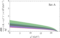
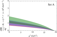
Figure 1: Differential branching fraction ${dBR(B_{s}\to\eta^{(\prime)}\ell^{+}\ell^{-})/dq^{2}}$ ($\ell=e,\mu$) as a function of the momentum transfer $q^{2}$ (upper plots), and branching fraction $BR(B_{s}\to\eta^{(\prime)}\ell^{+}\ell^{-})$ versus the compatification scale $\displaystyle{R^{-1}}$ (lower plots) obtained using set A and B of form factors. In each upper plot the lowest (red) region is obtained in SM ($1/R\to\infty$), the intermediate (blue) region for the compactification scale $1/R=500$ GeV and the uppermost (green) region for $1/R=200$ GeV.

The results obtained using the form factor $\xi^{B\to K}$ in the SCET framework are affected by the largest uncertainty and encompass the predictions based on the set A and set B. We consider these results as the most conservative determinations of the decay rates, as well as for the other observables.

The results from set A and B are compatible within the errors, with lower central values for set A. The uncertainties, estimated at the level of 30% in the rates for each set of form factor, become higher when the central values are compared: the difference provides us with hints on the level of improvement in the determination of the form factors needed at present. Such an improvement also concernes other determinations of the form factors Skands:2000ru .

As a further remark, we notice that the KLOE fit of the $\eta-\eta^{\prime}$ mixing eq.(12) corresponds to using an effective mixing angle $\varphi^{eff}=(44.5\pm 1.5)^{\circ}$ in the expressions of the $B_{s}\to\eta^{\prime}$ form factors, and to a $10\%$ decrease of the corresponding decay rates.

It is worth comparing the predictions (26)-(27) with the results quoted by the Heavy Flavour Averaging Group (HFAG) for the analogous $B$ decay modes HFAG : ${BR}(B^{0}\to K^{0}\ell^{+}\ell^{-})=\big{(}3.2^{+0.8}_{-0.6}\big{)}\times 10^{-7}$ and ${BR}(B^{+}\to K^{+}\ell^{+}\ell^{-})=(4.9\pm 0.5)\times 10^{-7}$ for $\ell=e,\mu$. On the other hand, in the approach based on the QF mixing scheme, a relation connecting the decay width of $B_{s}\to\eta\ell^{+}\ell^{-}$ to that of $B_{s}\to K^{0}\ell^{+}\ell^{-}$ induced by the transition $b\to d$:

$${BR(B_{s}\to K^{0}\ell^{+}\ell^{-})\over BR(B_{s}\to\eta\ell^{+}\ell^{-})}={1\over(\sin\varphi)^{2}}\left|{V_{td}\over V_{ts}}\right|^{2}(1+\Delta_{SU(3)}+\Delta^{\prime})\,\,\,,$$ (30)

involves an $SU(3)$ correction term $\Delta_{SU(3)}$ (presumably small) and a term $\Delta^{\prime}$ coming from the additional contribution proportional to $V_{ub}V^{*}_{ud}$, the correspondent of which has been neglected in the effective Hamiltonian (2) in case of $b\to s$ modes. Such a kind of relations is of great interest, both from the theoretical and the experimental viewpoint, and deserves a dedicated analysis.

In the ACD model the Wilson coefficients $C_{7}^{eff}$, $C_{9}$ and $C_{10}$ depend on the compactification scale $1/R$, hence decay rates and distributions vary with this parameter. $C_{7}^{eff}$ depends on $1/R$ through two functions $D^{\prime}(x_{t},{1\over R})$ and $E^{\prime}(x_{t},{1\over R})$ representing the contribution of $\gamma$-penguins and chromomagnetic penguins, respectively. The contribution of $Z^{0}$-penguins enters in the functions $Y(x_{t},{1\over R})$, $Z(x_{t},{1\over R})$ and $X(x_{t},{1\over R})$: $Y$ and $Z$ determine the coefficient $C_{9}$, while $C_{10}$ depends only on $Y$. As for the function $X$, it enters in the ACD expression of the coefficient $C_{L}$ relevant for the modes with neutrinos discussed in the next Section.

These functions obey the general representation (6), and can be found, e.g., in buras ; noi . For values of the compactification scale $1/R$ of a few hundreds of GeV the coefficient $C_{7}^{eff}$ is suppressed in the ACD model with respect to the SM value, while $C_{10}$ is enhanced and $C_{9}$ turns out to be almost unaffected. For example, at ${1\over R}=300$ GeV one has: $\displaystyle{C_{7}^{eff,ACD}\over C_{7}^{eff,SM}}\simeq 0.82$,$\displaystyle{C_{9}^{ACD}\over C_{9}^{SM}}\simeq 1.01$, $\displaystyle{C_{10}^{ACD}\over C_{10}^{SM}}\simeq 1.16$. As a consequence, for the decay into $\eta$ and $m_{\ell}=0$ we find for the function $p(q^{2})$ in (24) at $q^{2}=q^{2}_{max}$ and $1/R=300$ GeV: $\displaystyle{p(q^{2}_{max})|_{1/R=300\,{\rm GeV}}\over p(q^{2}_{max})|_{SM}}=1.23-1.42$, depending on the set of form factors.

The dependence of the rates on $1/R$ is obscured by the uncertainty of the hadronic form factors, as shown in Fig. 1, at values of this scale excluded by the analyses of the electroweak constraints: $1/R\geq 250$ GeV. Sensitivity of the decay rate to $1/R$ could be achieved by a reduction in the hadronic uncertainty of about a factor of two: in this case, the measurement of the rates of $B_{s}\to\eta^{(\prime)}\ell^{+}\ell^{-}$ would allow to exclude the $1/R$ region below $350-400$ GeV, keeping the same uncertainties quoted for the other input parameters. Concerning the differential distributions ${d\Gamma\over dq^{2}}(B_{s}\to\eta\ell^{+}\ell^{-})$ and ${d\Gamma\over dq^{2}}(B_{s}\to\eta^{\prime}\ell^{+}\ell^{-})$ also depicted in Fig.1, the enhancement at small values of dilepton invariant mass obtained for decreasing compactification scales $1/R$ could be observed after the same improvement of the accuracy of the form factors.

A possibility to reduce the effects of the hadronic uncertainties consists in comparing the decay distributions of $B_{s}\to\eta\ell^{+}\ell^{-}$ and $D_{s}\to\eta\ell^{+}\nu_{\ell}$ ($\ell=e,\mu$) at large values of momentum transfer $q^{2}\simeq q^{2}_{max}$, i.e. close to the end-point. In this range the ratio:

$$R(y)={{d\Gamma(B_{s}\to\eta\ell^{+}\ell^{-})/dy}\over{d\Gamma(D_{s}\to\eta\ell^{+}\nu_{\ell})/dy}}$$ (31)

obtained evaluating the distributions at the same value of $y={E\over M_{\eta}}$ can be written, up to corrections ${\cal O}({1\over m_{c}}-{1\over m_{b}})$, as:

$$R(y) = \left|{V_{tb}V^{*}_{ts}\over V_{cs}}\right|^{2}{\alpha^{2}\over 8\pi^{2}}\left({M_{B_{s}}\over M_{D_{s}}}\right)^{2}$$

$$\left(|C_{10}|^{2}+\left|C_{9}-{2(m_{b}+m_{s})\over M_{B_{s}}+M_{\eta}}c_{7}^{eff}{F_{T}^{B_{s}\to\eta}(y)\over F_{1}^{B_{s}\to\eta}(y)}\right|^{2}\right)$$

thus providing an access to the Wilson coefficients $C_{7,9}$ and $C_{10}$, since the ratio of $F_{T}^{B_{s}\to\eta}(y)\over F_{1}^{B_{s}\to\eta}(y)$ is practically independent of $y$ and of the set of form factors. To further reduce the impact of the hadronic corrections, the double ratio could be considered:

$$\tilde{R}(y)=\left[{{d\Gamma(B_{s}\to\eta\ell^{+}\ell^{-})/dy}\over{d\Gamma(D_{s}\to\eta\ell^{+}\nu_{\ell})/dy}}\right]/\left[{{d\Gamma(B_{s}\to K\ell^{+}\nu)/dy}\over{d\Gamma(D_{s}\to K\ell^{+}\nu_{\ell})/dy}}\right]\\$$ (33)

which is given by

$$\tilde{R}(y) = \left|{V_{tb}V^{*}_{ts}\over V_{cs}}\right|^{2}\left|{V_{cd}\over V_{ub}}\right|^{2}{\alpha^{2}\over 8\pi^{2}}\left({M_{B_{s}}\over M_{D_{s}}}\right)^{2}$$

$$\left(|C_{10}|^{2}+\left|C_{9}-{2(m_{b}+m_{s})\over M_{B_{s}}+M_{\eta}}c_{7}^{eff}{F_{T}^{B_{s}\to\eta}(y)\over F_{1}^{B_{s}\to\eta}(y)}\right|^{2}\right)$$

up to corrections ${\cal O}(m_{s}\left({1\over m_{c}}-{1\over m_{b}}\right))$ grinstein . However, the double ratio involves many CKM suppressed transitions, and its measurement is challenging.

V $B_{s}\to\eta\nu\bar{\nu}$ and $B_{s}\to\eta^{\prime}\nu\bar{\nu}$

The exclusive decays with two neutrinos in the final state, which from the theoretical side are among the cleanest FCNC processes, require only one hadronic form factor. The observables are the decay distributions and the total decay widths. For the former, it is convenient to use the variable $\displaystyle x={E_{miss}\over M_{B_{s}}}$, with $E_{miss}$ the energy of the neutrino pair in the $B_{s}$ rest frame (missing energy), with $\displaystyle{0.5\leq x\leq 1-{M_{\eta^{(\prime)}}\over M_{B_{s}}}}$. In terms of the variable $x$ the differential decay rate $\displaystyle{d\Gamma\over dx}$ reads:

$${d\Gamma(B_{s}\to\eta^{(\prime)}\nu\bar{\nu})\over dx}\hskip 142.26378pt$$

$$=3\;{|C_{L}|^{2}\,|F^{B_{s}\to\eta^{(\prime)}}_{1}(q^{2})|^{2}\over 48\pi^{3}M_{B_{s}}}\sqrt{\lambda^{3}(q^{2},M_{B_{s}}^{2},M_{\eta^{(\prime)}}^{2})}\;,\hskip 14.22636pt$$ (35)

with the invariant mass $q^{2}$ of the neutrino pair expressed in terms of $x$: $q^{2}=M_{B_{s}}^{2}(2x-1)+M_{\eta^{(\prime)}}^{2}$. $C_{L}$ is the Wilson coefficient in (4) and the factor of $3$ corresponds to the sum over the three neutrino flavours.

The differential branching fraction is plotted in Fig. 2 in the case of $\eta$ and $\eta^{\prime}$ , respectively, for the sets A and B of form factors. In the Standard Model one predicts:

$${BR}(B_{s}\to\eta\nu\bar{\nu})=\left\{\begin{array}[]{lll}(0.95\pm 0.2)\times 10^{-6}\hskip 8.5359pt{\rm set\,A}\\ (2.2\pm 0.7)\times 10^{-6}\hskip 14.22636pt{\rm set\,B}\\ (2.9\pm 1.5)\times 10^{-6}\hskip 14.22636pt{\rm set\,C}\hskip 2.0pt\end{array}\right.$$ (36)

$${BR}(B_{s}\to\eta^{\prime}\nu\bar{\nu})=\left\{\begin{array}[]{lll}(0.9\pm 0.2)\times 10^{-6}\hskip 11.38092pt{\rm set\,A}\\ (1.9\pm 0.5)\times 10^{-6}\hskip 11.38092pt{\rm set\,B}\\ (2.4\pm 1.3)\times 10^{-6}\hskip 11.38092pt{\rm set\,C}\hskip 2.0pt\end{array}\right.$$ (37)

These predictions can be compared to the present upper bounds for the corresponding $B\to K\nu\bar{\nu}$ modes, quoted by HFAG: ${BR}(B^{0}\to K^{0}\nu\bar{\nu})<160\times 10^{-6}$ and ${BR}(B^{+}\to K^{+}\nu\bar{\nu})<14\times 10^{-6}$ HFAG , which are compatible with the SM expectations scrimieri1 .

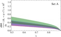
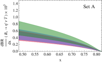
Figure 2: Differential decay rates ${dBR(B_{s}\to\eta^{(\prime)}\nu\bar{\nu})/dx}$ as a function of ${x={E_{miss}/M_{B_{s}}}}$ (upper plots), and branching fractions $BR(B_{s}\to\eta^{(\prime)}\nu\bar{\nu})$ versus $R^{-1}$ (lower plots) obtained using set A and B (right) of form factors. In the upper plots the lowest region is obtained in SM; the intermediate (blue) one for $1/R=500$ GeV, the uppermost (green) one for $1/R=200$ GeV.

In the ACD model, the coefficient is slightly enhanced: for example $\displaystyle{C_{L}^{ACD}\over C_{L}^{SM}}\simeq 1.10$ at $1/R=300$ GeV. However, the $1/R$ dependence of the branching fractions is obscured by the hadronic uncertainty, as shown in Fig. 2. The distribution in missing energy shows an enhancement at small values of $x$ which becomes sizeable at the lowest values of the $1/R$ range, $1/R\sim 250$ GeV. The presence of two neutrinos in the final state makes the measurements of these modes a challenge that can be faced at an $e^{+}e^{-}$ superB factory operating at the $\Upsilon(5S)$ peak.

VI The $bs$ UT triangle in ACD

To complete our discussion about $B_{s}$ physics in the ACD model, we turn to the bs unitarity triangle (UT) and, in particular, to the weak phase $\beta_{s}$ defined as: $\beta_{s}=Arg\left[-\displaystyle{V_{ts}V_{tb}^{*}\over V_{cs}V_{cb}^{*}}\right]$. Being ACD a Minimal Flavour Violation model, the CKM matrix has the same structure as in the SM: it is constrained to be unitary and is described in terms of four parameters, one of which is a complex phase: $\rho$, $\eta$, A and $\lambda$ in the Wolfenstein parameterization Wolfenstein:1983yz . At O($\lambda^{3}$) only $V_{ub}$ and $V_{td}$ have a complex phase, while at O($\lambda^{4}$) also $V_{ts}$ is complex and its argument identifies $\beta_{s}$ Buras:1994ec .

As it is well known, the various unitarity conditions are represented as triangles in the complex plane. Even though the CKM matrix has the same structure in ACD and SM, and, in particular, its phase is in both cases the only source of CP violation, it may happen that the various CKM elements differ in the two models and therefore the UT triangles do not coincide. Deviations could be expected for elements extracted from loop-induced processes, where the tower of KK modes may play a role; for elements obtained from tree level decays no difference is expected, as for $|V_{us}|$, $|V_{ub}|$ and $|V_{cb}|$. For the db triangle defined by the relation: $V_{ud}V_{ub}^{*}+V_{cd}V_{cb}^{*}+V_{td}V_{tb}^{*}=0$, only the side $R_{t}=\displaystyle{|V_{td}V_{tb}^{*}|\over|V_{cd}V_{cb}^{*}|}$ depends on $R^{-1}$ through the dependence of $|V_{td}|$ coming from the KK contribution to the $B_{d}^{0}-{\bar{B}}_{d}^{0}$ mixing buras . Using such a result, together with the measured value of $\displaystyle{|V_{ub}|\over|V_{cb}|}$, the variation of $\bar{\rho}=\left(1-{\lambda^{2}\over 2}\right)\rho$, $\bar{\eta}=\left(1-{\lambda^{2}\over 2}\right)\eta$, and of $\gamma$ (the phase of $V^{*}_{ub}$) has been obtained buras , finding that the db triangle in the ACD model could be slightly different than in the SM.

Figure 3: CKM element $V_{ts}$ (left) and phase $\beta_{s}$ (rad) (right) versus $R^{-1}$.

The bs triangle stems from the unitarity condition involving CKM elements relevant for $B_{s}$ decays, and is defined by the relation:

$$V_{us}V_{ub}^{*}+V_{cs}V_{cb}^{*}+V_{ts}V_{tb}^{*}=0\,\,.$$ (38)

Analogously to $V_{td}$, $V_{ts}$ inherits the $R^{-1}$ dependence from $B_{s}^{0}-{\bar{B}}_{s}^{0}$ mixing buras : $\Delta M_{s}\propto S(x_{t},1/R)|V_{ts}|^{2}$, where the proportionality factor does not depend on $R^{-1}$ and is common to ACD and SM. The function $S(x_{t},1/R)$ takes into account the SM contribution, $S_{0}(x_{t})$, and the contribution of the KK modes: $S(x_{t},1/R)=S_{0}(x_{t})+\sum_{n}S_{n}(x_{t},1/R)$, with:

$$\sum_{n}S_{n}(x_{t},x_{n})= - {x_{t}(5-10x_{t}+x_{t}^{2})\over 8(x_{t}-1)^{2}}+{\pi M_{W}R\over 2}\Big{\{}-{x_{t}(3x_{t}-1)\over 2(x_{t}^{2}-1)^{3}}J(R,-1/2)+{(1-3x_{t}+7x_{t}^{2}-x_{t}^{3})\over 2(x_{t}-1)^{3}}J(R,1/2)$$ (39)

$$- {(-3+6x_{t}-x_{t}^{3})\over 2x_{t}(x_{t}-1)^{3}}J(R,3/2)+{1\over 2x_{t}}\int_{0}^{1}dy\,[x_{t}+3(1+x_{t})y]\sqrt{y}\,{\rm ctanh}(\pi M_{W}R\sqrt{y})\Big{\}}$$

and

$$J(R,\alpha)=\int_{0}^{1}dyy^{\alpha}\big{[}{\rm ctanh}(\pi M_{W}R\sqrt{y})-x_{t}^{1+\alpha}{\rm ctanh}(\pi m_{t}R\sqrt{y})\big{]}.$$ (40)

As a consequence one finds:

$$|V_{ts}|_{ACD}=|V_{ts}|_{SM}\sqrt{\displaystyle{S_{0}(x_{t})\over S(x_{t},1/R)}}\,\,\,.$$ (41)

In Fig.3 we show the dependence of $|V_{ts}|_{ACD}$ on $R^{-1}$ using the quoted value of $|V_{ts}|_{SM}$. Since at O($\lambda^{4}$) $V_{ts}=-A\lambda^{2}+{A\lambda^{4}\over 2}[1-2\rho-2i\eta]$, it turns out that $\beta_{s}=\arctan\left[\displaystyle{2\lambda^{2}\eta\over 2-\lambda^{2}(1-2\rho)}\right]$. Using the dependence of $\rho$ and $\eta$ (or $\bar{\rho}$ and $\bar{\eta}$), also the $\beta_{s}$ dependence on $R^{-1}$ can be obtained; it is depicted in Fig. 3. The SM result for $\beta_{s}$ is small: $\beta_{s}\simeq 0.019$ rad, and the dependence on the compactification scale $R^{-1}$ further reduces this value. As mentioned in the Introduction, preliminary Tevatron results point towards larger values of $\beta_{s}$, so that our analysis supports the conclusion that a confirmation of the measurement of a large phase in the $B_{s}$ mixing would point towards new Physics models different from MFV scenarios.

In Fig. 4 the rescaled ${\it bs}$ UT triangle in the ACD model is displayed at the representative compactification scale $R^{-1}=300$ GeV.

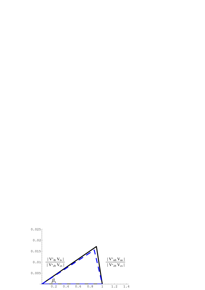
Figure 4: Rescaled ${\it bs}$ UT triangle in the SM (continuous line) and the ACD model at $R^{-1}=300$ GeV (dashed line).

VII Conclusions

Together with other rare $B_{s}$ decays, the loop-induced transitions $B_{s}\to\eta^{(\prime)}\ell^{+}\ell^{-}$ and $B_{s}\to\eta^{(\prime)}\nu\bar{\nu}$ must be included in the Physics programmes of experiments aimed at performing tests of the Standard Model and at searching signals of new Physics like those related to extra dimensions. Within SM, using the flavour scheme for the $\eta-\eta^{\prime}$ mixing and the angle determined by the KLOE Collaboration from radiative $\phi$ decays, we have predicted decay widths and distributions of these rare $B_{s}$ channels. The results for the branching fractions of modes with two charged leptons are ${\cal O}(10^{-7})$ for $\ell=e,\mu$ and ${\cal O}(10^{-8})$ for $\ell=\tau$, suggesting that they are within the reach of facilities like a SuperB factory. In the case of the final states with two neutrinos, the branching ratios are of ${\cal O}(10^{-6})$. The uncertainty in the numerical results is dominated by the error of the hadronic form factors: in order to be sensitive to compactification scales $1/R\sim 350-400$ GeV in the ACD model the error in the form factors should be reduced by about a factor of two.

A remark concerns the issue of the $\eta-\eta^{\prime}$ mixing. In addition to modes with light mesons, processes involving heavy mesons provide information on this mixing. Examples are the $J/\psi$ radiative decays: $J/\psi\to\eta^{\prime}\gamma$ and $J/\psi\to\eta\gamma$, which are sensitive to the glue content of $\eta$ and $\eta^{\prime}$ Ball:1995zv . Although experimentally challenging and considered mainly for different purposes, also the ratio $\displaystyle{{BR}(B_{s}\to\eta^{\prime}\ell^{+}\ell^{-})\over{BR}(B_{s}\to\eta\ell^{+}\ell^{-})}$ represents a possibility to determine $\varphi$ and to look at the gluonic content of $\eta^{\prime}$. A discrepancy in the comparison of the determination of the same quantity from other channels, e.g. from the ratio $\displaystyle{{BR}(\phi\to\eta^{\prime}\gamma)\over{BR}(\phi\to\eta\gamma)}$, would signal peculiar effects in $B_{s}\to\eta^{(\prime)}$ modes.

Acknowledgments

FDF thanks Thorsten Feldmann and Tobias Hurth for collaboration on light-cone QCD sum rules in the SCET framework. This work was supported in part by the EU contract No. MRTN-CT-2006-035482, ”FLAVIAnet”.

References

• (1) P. Ball et al., “$B$ Decays at the LHC,” arXiv:hep-ph/0003238; K. Anikeev et al., “$B$ physics at the Tevatron: Run II and beyond,” arXiv:hep-ph/0201071; M. Bona et al., “SuperB: A High-Luminosity Asymmetric $e^{+}e^{-}$ Super Flavor Factory. Conceptual Design Report,” arXiv:0709.0451 [hep-ex]; M. Artuso et al., “$B$, $D$ and $K$ Decays”, Eur. Phys. J. C57, 309 (2008).
• (2) V. M. Abazov et al. [D0 Collaboration], Phys. Rev. Lett.  98, 121801 (2007); Phys. Rev.  D 76, 057101 (2007); T. Aaltonen et al. [CDF collaboration], Phys. Rev. Lett.  100, 121803 (2008); Phys. Rev. Lett.  100, 161802 (2008).
• (3) A. Drutskoy, arXiv:0905.2959 [hep-ex].
• (4) T. Appelquist, H. C. Cheng and B. A. Dobrescu, Phys. Rev.  D 64, 035002 (2001).
• (5) T. Appelquist and H. U. Yee, Phys. Rev.  D 67, 055002 (2003).
• (6) H. C. Cheng, K. T. Matchev and M. Schmaltz, Phys. Rev.  D 66, 036005 (2002), Phys. Rev.  D 66, 056006 (2002); G. Servant and T. M. P. Tait, Nucl. Phys.  B 650, 391 (2003).
• (7) For a review see: D. Hooper and S. Profumo, Phys. Rept.  453, 29 (2007).
• (8) A. J. Buras, M. Spranger and A. Weiler, Nucl. Phys.  B 660, 225 (2003); A. J. Buras, A. Poschenrieder, M. Spranger and A. Weiler, Nucl. Phys.  B 678, 455 (2004).
• (9) P. Colangelo, F. De Fazio, R. Ferrandes and T. N. Pham, Phys. Rev.  D 73, 115006 (2006); Phys. Rev.  D 74, 115006 (2006); Phys. Rev.  D 77, 055019 (2008).
• (10) U. Haisch and A. Weiler, Phys. Rev.  D 76, 034014 (2007).
• (11) R. Mohanta and A. K. Giri, Phys. Rev.  D 75, 035008 (2007); T. M. Aliev and M. Savci, Eur. Phys. J.  C 50, 91 (2007); T. M. Aliev, M. Savci and B. B. Sirvanli, Eur. Phys. J.  C 52, 375 (2007); I. Ahmed, M. A. Paracha and M. J. Aslam, Eur. Phys. J.  C 54, 591 (2008); A. Saddique, M. J. Aslam and C. D. Lu, Eur. Phys. J.  C 56, 267 (2008); V. Bashiry and K. Zeynali, Phys. Rev.  D 79, 033006 (2009); Y. M. Wang, M. J. Aslam and C. D. Lu, Eur. Phys. J.  C 59, 847 (2009).
• (12) G. Devidze, A. Liparteliani and U. G. Meissner, Phys. Lett.  B 634, 59 (2006); I. I. Bigi, G. G. Devidze, A. G. Liparteliani and U. G. Meissner, Phys. Rev.  D 78, 097501 (2008).
• (13) C. Bobeth, M. Misiak and J. Urban, Nucl. Phys. B 574, 291 (2000); H. H. Asatrian, H. M. Asatrian, C. Greub and M. Walker, Phys. Lett. B 507, 162 (2001); Phys. Rev. D 65, 074004 (2002); Phys. Rev. D 66, 034009 (2002); H. M. Asatrian, K. Bieri, C. Greub and A. Hovhannisyan, Phys. Rev. D 66, 094013 (2002); A. Ghinculov, T. Hurth, G. Isidori and Y. P. Yao, Nucl. Phys. B 648, 254 (2003); A. Ghinculov, T. Hurth, G. Isidori and Y. P. Yao, Nucl. Phys. B 685, 351 (2004); C. Bobeth, P. Gambino, M. Gorbahn and U. Haisch, JHEP 0404, 071 (2004).
• (14) T. Inami and C. S. Lim, Prog. Theor. Phys.  65, 297 (1981) [Erratum-ibid.  65, 1772 (1981)].
• (15) G. Buchalla and A. J. Buras, Nucl. Phys. B 400, 225 (1993); G. Buchalla, A. J. Buras and M. E. Lautenbacher, Rev. Mod. Phys.  68, 1125 (1996).
• (16) M. Misiak and J. Urban, Phys. Lett.  B 451, 161 (1999).
• (17) G. Buchalla and A. J. Buras, Nucl. Phys. B 548, 309 (1999).
• (18) T. Feldmann, P. Kroll and B. Stech, Phys. Rev.  D 58, 114006 (1998); Phys. Lett.  B 449, 339 (1999); T. Feldmann, Int. J. Mod. Phys.  A 15, 159 (2000).
• (19) F. De Fazio and M. R. Pennington, JHEP 0007, 051 (2000).
• (20) R. Escribano, Acta Phys. Polon. Supp.  2, 71 (2009).
• (21) F. Ambrosino et al. [KLOE Collaboration], Phys. Lett. B 648, 267 (2007).
• (22) M. B. Wise, Phys. Rev.  D 45, 2188 (1992).
• (23) C. Amsler et al. [Particle Data Group], Phys. Lett.  B 667, 1 (2008).
• (24) For a review see: P. Colangelo and A. Khodjamirian, arXiv:hep-ph/0010175.
• (25) P. Colangelo, F. De Fazio, P. Santorelli and E. Scrimieri, Phys. Rev.  D 53, 3672 (1996) [Erratum-ibid.  D 57, 3186 (1998)].
• (26) P. Ball and R. Zwicky, Phys. Rev.  D 71, 014015 (2005).
• (27) C. W. Bauer, S. Fleming, D. Pirjol and I. W. Stewart, Phys. Rev. D 63, 114020 (2001); C. W. Bauer and I. W. Stewart, Phys. Lett. B 516, 134 (2001); M. Beneke, A. P. Chapovsky, M. Diehl and T. Feldmann, Nucl. Phys. B 643, 431(2002); M. Beneke and T. Feldmann, Phys. Lett. B 553, 267 (2003).
• (28) F. De Fazio, T. Feldmann and T. Hurth, Nucl. Phys.  B 733, 1 (2006) [Erratum-ibid.  B 800, 405 (2008)]; JHEP 0802, 031 (2008).
• (29) M. Beneke and M. Neubert, Nucl. Phys.  B 651, 225 (2003).
• (30) Y. Y. Charng, T. Kurimoto and H. n. Li, Phys. Rev.  D 74, 074024 (2006) [Phys. Rev.  D 78, 059901 (2008)].
• (31) P. Ball and G. W. Jones, JHEP 0708, 025 (2007).
• (32) A. Ali and A. Y. Parkhomenko, Eur. Phys. J.  C 30, 183 (2003).
• (33) A. R. Williamson and J. Zupan, Phys. Rev.  D 74, 014003 (2006) [Erratum-ibid.  D 74, 03901 (2006)].
• (34) C. H. Chen and C. Q. Geng, Phys. Lett.  B 645, 197 (2007).
• (35) P. Z. Skands, JHEP 0101, 008 (2001); C. Q. Geng and C. C. Liu, J. Phys. G 29, 1103 (2003).
• (36) E. Barberio et al. [Heavy Flavor Averaging Group], arXiv:0808.1297 [hep-ex].
• (37) B. Grinstein and D. Pirjol, Phys. Lett.  B 549, 314 (2002).
• (38) P. Colangelo, F. De Fazio, P. Santorelli and E. Scrimieri, Phys. Lett.  B 395, 339 (1997); G. Buchalla, G. Hiller and G. Isidori, Phys. Rev.  D 63, 014015 (2001); W. Altmannshofer, A. J. Buras, D. M. Straub and M. Wick, JHEP 0904, 022 (2009).
• (39) L. Wolfenstein, Phys. Rev. Lett.  51, 1945 (1983).
• (40) A. J. Buras, M. E. Lautenbacher and G. Ostermaier, Phys. Rev.  D 50, 3433 (1994).
• (41) P. Ball, J. M. Frere and M. Tytgat, Phys. Lett.  B 365, 367 (1996).