Non-Gaussian entanglement distillation for continuous variables

Abstract

Entanglement distillation is an essential ingredient for long distance quantum communications Briegel et al. (1998). In the continuous variable setting, Gaussian states play major roles in quantum teleportation, quantum cloning and quantum cryptography Braunstein and van Loock (2005). However, entanglement distillation from Gaussian states has not yet been demonstrated. It is made difficult by the no-go theorem stating that no Gaussian operation can distill Gaussian states Eisert et al. (2002); Fiurášek (2002); Giedke and Cirac (2002). Here we demonstrate the entanglement distillation from Gaussian states by using measurement-induced non-Gaussian operations, circumventing the fundamental restriction of the no-go theorem. We observed a gain of entanglement as a result of conditional local subtraction of a single photon or two photons from a two-mode Gaussian state. Furthermore we confirmed that two-photon subtraction also improves Gaussian-like entanglement as specified by the Einstein-Podolsky-Rosen (EPR) correlation. This distilled entanglement can be further employed to downstream applications such as high fidelity quantum teleportation Opatrný et al. (2000) and a loophole-free Bell test García-Patrón et al. (2004).

Long distance quantum communications rely on the ability to faithfully distribute entanglement between distant locations. However, inevitable decoherence and the inability to amplify quantum signals hinder efforts to extend a quantum optical link to the practically large scale. To overcome this difficulty, entanglement distillation can be used - a protocol in which each distant party locally manipulates particles of less entangled pairs with the aid of classical communication to extract a smaller number of pairs of higher entanglement Bennett et al. (1996). In discrete variable systems many distillation experiments have already been demonstrated Kwiat et al. (2001); Pan et al. (2001); Yamamoto et al. (2003); Reichle et al. (2006).

An alternative to the discrete variable system is the one described by continuous variables (CV), typically represented by the quadrature amplitudes of a light field. For CV quantum information, Gaussian states and Gaussian operations Ferraro et al. (2005) are of particular importance. They are readily available in the laboratory and serve as a complete framework for many quantum protocols Braunstein and van Loock (2005). The first experiments of CV entanglement distillation were reported in Hage et al. (2008); Dong et al. (2008). These two works rely on Gaussian operations. However, it was theoretically proven that Gaussian operations can never distill entanglement from Gaussian state inputs – this is known as the no-go theorem of Gaussian operations Eisert et al. (2002); Fiurášek (2002); Giedke and Cirac (2002). In Hage et al. (2008); Dong et al. (2008), the inputs had been subjected to some specific classes of non-Gaussian noise, such as phase-diffusion Hage et al. (2008) or temporally varying attenuation Dong et al. (2008). In those cases, well established Gaussian technologies can be applied to distill the entanglement.

So far, there has been no demonstration of entanglement distillation with Gaussian inputs. This task essentially requires a new technology of non-Gaussian operations. Recent theories also revealed that this is a must to realize quantum speed-up of CV quantum information processing (QIP) Bartlett et al. (2002). Triggered by this new paradigm of non-Gaussian QIP, the research field extending to the non-Gaussian regime has rapidly developed Ourjoumtsev et al. (2006); Neergaard-Nielsen et al. (2006); Wakui et al. (2007). The increase Ourjoumtsev et al. (2007) and preparation Ourjoumtsev et al. (2009) of entanglement from Gaussian inputs by non-local photon subtraction were also demonstrated. These are important steps towards the realization of entanglement distillation from Gaussian states.

Here we report on the entanglement distillation directly from CV Gaussian states by using local photon subtraction as non-Gaussian operations, circumventing the no-go restriction on Gaussian operations. A schematic of our experiment is depicted in Fig. 1. A continuous wave squeezed vacuum is generated from an optical parametric oscillator (OPO) detailed elsewhere Wakui et al. (2007). The initial Gaussian entangled state is prepared by splitting the squeezed vacuum by half at the first beam splitter and is distributed to the separate parties, Alice and Bob. This half-split squeezed vacuum with squeezing parameter $r$ is effectively equivalent to the two-mode squeezed vacuum with $r/2$ (they are compatible by local unitary operations. see Appendix A.2). At each site of Alice and Bob, a probabilistic non-Gaussian operation – photon subtraction – is performed. Specifically, a small part of the beam is picked off by a polarizing beam splitter with the variable reflectance $R$ and sent through filtering cavities Wakui et al. (2007) to an avalanche photodiode (APD) to detect a photon (Fig. 1). Each photon detection at the APD heralds a local success of the photon subtraction attempt. Conditioned on the subtraction of a photon by a single party (single-photon subtraction) or the simultaneous subtraction of a photon by both parties (two-photon subtraction), Alice and Bob retain those two-mode states which have successfully had their entanglement increased. While the single-photon subtraction scheme will have a higher success rate, the two-photon subtraction scheme will give a more Gaussian-like final state which is more readily applicable to further processing such as e.g. quantum teleportation.

The distillation works since the local photon subtraction changes the non-local unfactorizable correlations of the initial state. To see this intuitively, let us describe the initial squeezed state with squeezing parameter $r$ in photon number basis as $\left|0,0\right\rangle-\frac{\lambda}{2\sqrt{2}}(\left|0,2\right\rangle+\sqrt{2}\left|1,1\right\rangle+\left|2,0\right\rangle)+O(\lambda^{2})$ where $|m,n\rangle=|m\rangle_{A}|n\rangle_{B}$, $\lambda=\tanh r$ and we omitted the normalization. For small $\lambda$, it is almost factorizable since $\left|0,0\right\rangle$ is dominant. Applying the single-photon subtraction, represented by an annihilation operator $\hat{a}$, the state is transformed to be $\sqrt{2}(\left|0,1\right\rangle+\left|1,0\right\rangle)+O(\lambda)$ which is clearly more entangled - the first Bell state term corresponds to 1 ebit of entanglement. We emphasize that the term $O(\lambda)$ is not negligible for larger $\lambda$ and critically contributes to the distillation, and thus the scheme works for any $\lambda$ in principle. See Appendix A.3 for the rigorous formulation and for the two-photon subtraction.

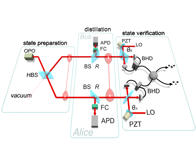
Figure 1: Schematic of the experiment. OPO: optical parametric oscillator, BS: beam splitter, HBS: half-beam splitter, BHD: balanced homodyne detector, LO: local oscillator, FC: filtering cavity, APD: avalanche photo diode, PZT: Piezo electric transducer. The phases of the LOs, $\theta_{A}$ and $\theta_{B}$ are stabilized by electronic feedback to the PZTs through field programmable gate array (FPGA) modules. The outputs of the BHDs are recorded by a digital oscilloscope triggered by either logical “AND” or “OR” of the click signals from the two APDs. For the state verification, a set of the homodyne outcomes are numerically converted into the “$+/-$” basis.

The verification of the distilled (or undistilled) states is carried out by a quantum tomographic method with two local homodyne measurements (see Fig. 1). For tomography, in general the local oscillator (LO) phases $\theta_{A}$ and $\theta_{B}$ (for Alice and Bob’s detectors, respectively) have to be swept over all possible combinations to collect full information of the two-mode state. In our case, however, it is significantly simplified due to the fact that our states, distilled or undistilled, are always represented in a decomposed way as

$$W(x_{A},p_{A},x_{B},p_{B}) =W_{s}(x_{-},p_{-})W_{v}(x_{+},p_{+}),$$ (1)

where $W$ is the Wigner function for the two-mode state, $x_{A},x_{B},p_{A},p_{B}$ are the quadrature amplitudes of modes $A$ and $B$, $x_{\pm}=\frac{x_{A}\pm x_{B}}{\sqrt{2}}$, $p_{\pm}=\frac{p_{A}\pm p_{B}}{\sqrt{2}}$ and $W_{s}$, $W_{v}$ are the Wigner functions for a (zero-, one-, or two-) photon subtracted squeezed vacuum and the vacuum respectively. For such a state, the scans of the homodyne measurements are necessary only for $\theta_{A}=\theta_{B}$ and the experimental data of $x_{\pm}$ is numerically obtainable from the measured $x_{A}$ and $x_{B}$ (Fig. 1). It should be stressed that although we assume the state factorization of (1), it can be directly assessed by verifying experimentally whether the state of the g+ h mode is indeed a pure vacuum state. For details, see Appendix A.1.

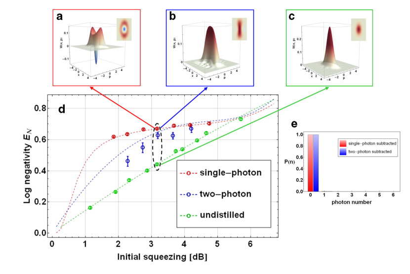
Figure 2: a, b, c Experimentally reconstructed Wigner functions and their contour plots of the “$-$” mode states for (a) Distilled state via single-photon subtraction with $R=$5%, (b) Distilled state via two-photon subtraction with $R=$10%, and (c) Undistilled initial state (squeezed vacuum with $R=$0%), all with initial squeezing of -3.2 dB. d Experimental logarithmic negativities as functions of the initial input squeezing. Here the initial squeezing refers to the squeezing of the states right after the OPO and is deduced from separately measured classical parametric amplification of the OPO. For the single-photon subtracted states (red) and the undistilled states (green), 600,000 samples over 6 phases were used for the reconstruction of each point. For the two-photon subtracted states (blue) 18,000 - 48,000 samples were used. The dashed curves are theoretical predictions based on independently measured experimental parameters. Every error bar represents an uncertainty of the state reconstruction and was estimated via a MonteCarlo simulation using the corresponding experimental parameters. e, The photon number distributions of the experimentally reconstructed “$+$” mode states corresponding to (a) and (b).

Examples of reconstructed Wigner functions obtained by the single- and two-photon subtractions, as well as the initial squeezed state are shown in Fig. 2a-c. The outputs of the homodyne detectors were sampled at 6 different phases of LO, namely $\theta_{A}=\theta_{B}=0,\pi/6,\pi/3,\pi/2,2\pi/3,5\pi/6$. We extract the measured values of the quadratures $\hat{x}_{A}$ and $\hat{x}_{B}$ by applying a mode function to the recorded traces Neergaard-Nielsen et al. (2006); Wakui et al. (2007); Takahashi et al. (2008). After calculating the corresponding values of $\hat{x}_{\pm}$, we reconstruct the density matrices for the “$+$” and “$-$” modes by the conventional maximum likelihood estimation Lvovsky (2004) without any correction of detection losses.

As shown in Fig. 2e, for the “$+$” mode states we got almost perfectly pure vacuum states with more than 99% accuracy. We confirmed that this holds irrespective of the initial squeezing level. This experimental evidence justifies our tomography scheme based on the relation (1). On the other hand, for the “$-$” mode states we observed two different kinds of non-Gaussian state depending on whether single photon or two photons were subtracted (Fig. 2a and b). They respectively correspond to the odd and even Schrödinger cat state, i.e. $\left|\alpha\right\rangle-\left|-\alpha\right\rangle$ and $\left|\alpha\right\rangle+\left|-\alpha\right\rangle$ where $\left|\alpha\right\rangle$ is a coherent state with coherent amplitude $\alpha$. Having these reconstructed states we can use the relation (1) backwards to calculate the amount of entanglement shared by Alice and Bob. Specifically, we calculate the logarithmic negativity $E_{\mathcal{N}}$ which is a monotone measure of entanglement Vidal and Werner (2002).

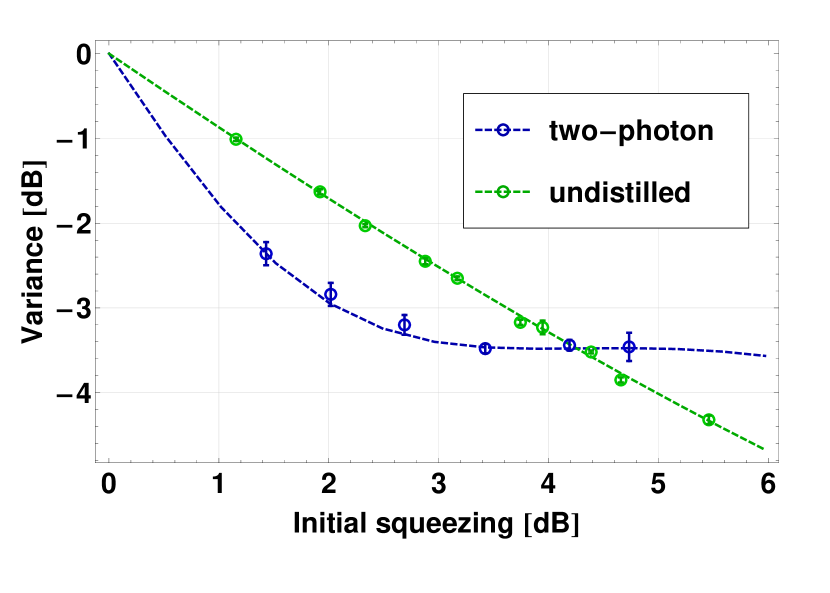
Figure 3: Squeezed variances of $x_{-}$ (normalized by the vacuum level). For the undistilled states each point was calculated from the full-reconstructed density matrices common to the negativity measurements. For the distilled states each point was obtained by directly measuring variance of 1,600 - 5,000 samples at the most squeezed phase.

Fig. 2d shows the experimental negativities of the undistilled Gaussian states, the states distilled by single-photon subtraction with $R=5\%$, and by two-photon subtraction with $R=10\%$ as functions of the squeezing of the initial input states. When evaluating negativity, one must take care of its strong dependency on the size of the data set. We investigated the behavior of the negativity on the data size and deduced an extrapolative value corresponding to an infinitely large data set for each point in Fig. 2d (See Appendix B). Note that without this analysis, evaluation of negativity with finite sized data very likely goes into an overestimate of the negativity. As shown in the figure, over a wide range of the initial squeezing we got clear gains of entanglement relative to the undistilled Gaussian states for both the single- and two-photon subtracted schemes.

A practical difference between the single- and two-photon subtracted scheme is on their rates of event detection. In the single-photon experiment the rate is around a few thousands per second, but in the two-photon experiment there are only a few events per second. So while for the former we can use hundreds of thousands of samples for the state reconstruction, for the latter we can only use a few tens of thousands limited by the long-term stability of the setup. In Fig. 2d the experimental negativities for the single-photon subtracted states and the undistilled states are in very good agreement with theory, but ones for the two-photon subtraction are slightly below the theoretical predictions. This may be due to an uncontrollable drift of the system during a long period of the measurements.

As can be seen in Fig. 2d, in terms of the logarithmic negativity the two-photon subtracted scheme does not have an advantage over the single-photon subtracted scheme despite its significantly lower success rate. However the two-photon subtracted distillation transforms a two-mode Gaussian state into one relatively close to a Gaussian state (see Fig. 2b). Hence one would expect that states distilled by this scheme still possess a Gaussian-like property of entanglement. For Gaussian states, two-mode entanglement is usually specified in terms of the Einstein-Podolsky-Rosen (EPR) correlation quantified by $\langle(\Delta\hat{x}_{-})^{2}\rangle\langle(\Delta\hat{p}_{+})^{2}\rangle$. Since the “$+$” mode is always a vacuum state (see Eq. 1), we can focus on the degree of squeezing of the “$-$” mode as an equivalent measure. We carried out measurements of the variance of $\hat{x}_{-}$ at its most squeezed phase conditioned on two-photon subtraction ( Fig. 3). Note that this measurement is considerably faster than reconstruction of a full state and is possibly more accurate due to its simplicity. The results in Fig. 3 show that the two-photon subtraction improves the EPR correlation of a state with up to 4 dB of initial squeezing. An improvement on the EPR correlation gives us an operational measure of success of the two-photon subtracted distillation in terms of the fidelity of CV quantum teleportation Opatrný et al. (2000). On the other hand, the single-photon subtracted distillation is never able to improve the degree of the EPR correlation. This fact demonstrates a clearly different nature of the distilled entanglement between the two schemes.

In conclusion, we have for the first time demonstrated CV entanglement distillation from Gaussian states by conditional local photon subtraction. Because of the importance of Gaussian states and the no-go theorem of the Gaussian distillation, this has been a long-standing experimental milestone to be achieved. Our scheme would serve as the de-Gaussifying process of a more generic distillation protocol proposed in Eisert et al. (2004) by combining it with the already demonstrated Gaussification processes Hage et al. (2008); Dong et al. (2008), which would realize long-distance CV quantum communications. Finally, our non-Gaussian entangled states are not only useful for communications but also for fundamental problems such as a loophole-free test of Bell’s inequality García-Patrón et al. (2004).

H.T. acknowledges the financial support from G-COE program commissioned by the MEXT of Japan.

Appendix A Theoretical description of the distilled states

A.1 Factorizability of the distilled states

Figure 4: a Schematic of the local photon subtraction. BS: beam splitter, HBS: half beam splitter. The letters A, B, C and D label the optical modes. The thinner lines represent the vacuum inputs. The gray boxes are photon detectors. Here the state of mode A is half-split and then photons are subtracted locally from the outputs of the HBS. b An equivalent model for a. The state of mode A is firstly photon-subtracted and then half-split with mode B.

Here we discuss the local photon subtraction from a two-mode entangled Gaussian state made by splitting a squeezed vacuum. Fig. 4a illustrates this scheme, where one of the inputs for the half-beam splitter is in the vacuum state. Conditioning on either photon detection at one of the detectors or coincidence detection of two detectors heralds a non-Gaussian two-mode state effectively described as follows (apart from the normalization).

$$\left|\psi_{out}\right\rangle_{AB} =\hat{a}_{A}^{n_{A}}\hat{a}_{B}^{n_{B}}\hat{B}_{AB}(\pi/4)\hat{S}_{A}(r)\left|0\right\rangle_{A}\left|0\right\rangle_{B}$$ (2)

$$=\hat{B}_{AB}(\pi/4)\,\hat{a}_{A}^{n_{A}+n_{B}}\hat{S}_{A}(r)\left|0\right\rangle_{A}\left|0\right\rangle_{B},$$ (3)

where $\hat{S}_{A}(r)$ is the squeezing operator with the squeezing parameter $r$ and $\hat{B}_{AB}(\pi/4)$ is the half-beam splitter operator for the modes $A$ and $B$. More generally we denote the beam splitter operator with reflectance $R$ as $\hat{B}_{AB}(\theta)$ where $\theta=\sin^{-1}(\sqrt{R})$ and $\hat{B}_{AB}(\theta)=\exp(\theta(\hat{a}^{\dagger}_{A}\hat{a}_{B}-\hat{a}_{A}\hat{a}^{\dagger}_{B})$). The integers $n_{A}$ and $n_{B}$ represent the number of photons subtracted, i.e. ($n_{A}$, $n_{B}$)=(1, 0) or (0, 1) for the single photon detection at either site and ($n_{A}$, $n_{B}$)=(1, 1) for the coincidence detection of both sites. The state given by (3) is a half-split state of the photon subtracted squeezed vacuum. Hence the situation described by Fig. 4a can be equivalently transformed to the one in Fig. 4b. Although the description of (2) for photon subtraction is only valid in the limit where the reflectance of the local tapping BS goes to zero, as will be shown in the following, the equivalency between Fig. 4a and b still holds even when the photon subtraction is not ideal, i.e. the reflectance of the BS is not infinitesimal.

Consider the situation in Fig. 4a again, with definitions of modes A, B, C, and D. Here we assume that the reflectance of the tapping BS is finite. The following operator identity holds:

$$\hat{B}_{AC}(\theta)\hat{B}_{BD}(\theta)\hat{B}_{AB}(\pi/4)$$

$$=\hat{B}_{AB}(\pi/4)\hat{B}_{AB}^{\dagger}(\pi/4)\hat{B}_{AC}(\theta)\hat{B}_{BD}(\theta)\hat{B}_{AB}(\pi/4)$$ (4)

$$=\hat{B}_{AB}(\pi/4)\hat{B}_{AB}^{\dagger}(\pi/4)$$

$$\qquad\times\exp\left(\theta(\hat{a}^{\dagger}_{A}\hat{a}_{C}-\hat{a}_{A}\hat{a}^{\dagger}_{C}+\hat{a}^{\dagger}_{B}\hat{a}_{D}-\hat{a}_{B}\hat{a}^{\dagger}_{D})\right)\hat{B}_{AB}(\pi/4)$$ (5)

$$=\hat{B}_{AB}(\pi/4)\exp\left(\theta\left(-\hat{a}_{A}\frac{\hat{a}^{\dagger}_{C}-\hat{a}^{\dagger}_{D}}{\sqrt{2}}+\hat{a}^{\dagger}_{A}\frac{\hat{a}_{C}-\hat{a}_{D}}{\sqrt{2}}\right.\right.$$

$$\qquad\left.\left.-\hat{a}_{B}\frac{\hat{a}^{\dagger}_{C}+\hat{a}^{\dagger}_{D}}{\sqrt{2}}+\hat{a}^{\dagger}_{B}\frac{\hat{a}_{C}+\hat{a}_{D}}{\sqrt{2}}\right)\right)$$ (6)

$$=\hat{B}_{AB}(\pi/4)\hat{B}_{CD}(\pi/4)\hat{B}_{AC}(\theta)\hat{B}_{BD}(\theta)\hat{B}_{CD}^{\dagger}(\pi/4),$$ (7)

where $\hat{B}_{ij}$ stands for the beam splitter operator for modes $i$ and $j$. Then for an arbitrary input state $\left|\Psi\right\rangle$ for mode A and the vacuum states for modes B, C, and D:

$$\hat{B}_{BD}(\theta)\hat{B}_{AC}(\theta)\hat{B}_{AB}(\pi/4)\left|\Psi\right\rangle_{A}\left|0\right\rangle_{B}\left|0\right\rangle_{C}\left|0\right\rangle_{D}$$

$$=\hat{B}_{AB}(\pi/4)\hat{B}_{CD}(\pi/4)\hat{B}_{AC}(\theta)\hat{B}_{BD}(\theta)\hat{B}_{CD}^{\dagger}(\pi/4)$$

$$\qquad\times\left|\Psi\right\rangle_{A}\left|0\right\rangle_{B}\left|0\right\rangle_{C}\left|0\right\rangle_{D}$$ (8)

$$=\hat{B}_{AB}(\pi/4)\hat{B}_{CD}(\pi/4)\hat{B}_{AC}(\theta)\left|\Psi\right\rangle_{A}\left|0\right\rangle_{B}\left|0\right\rangle_{C}\left|0\right\rangle_{D}$$ (9)

This establishes the equivalency between the models shown in Fig. 4a and b again. Therefore the final output state of the protocol is identical to a half-split of the photon subtracted squeezed vacuum.

Let us return to the form of (3) for simplicity. Then we immediately have

$$\hat{B}^{\dagger}(\pi/4)\left|\psi_{out}\right\rangle_{AB} =\hat{a}_{A}^{n_{A}+n_{B}}\hat{S}_{A}(r)\left|0\right\rangle_{A}\left|0\right\rangle_{B},$$ (10)

which means that if we let the conditional two-mode state be combined at a half-beam splitter it becomes disentangled and furthermore the outputs get separated as a photon subtracted squeezed vacuum and the vacuum. Introducing new variables

$$\hat{x}_{\pm}=\frac{\hat{x}_{A}\pm\hat{x}_{B}}{\sqrt{2}}\quad\hat{p}_{\pm}=\frac{\hat{p}_{A}\pm\hat{p}_{B}}{\sqrt{2}},$$ (11)

where $\hat{x}_{A,B}$ and $\hat{p}_{A,B}$ are the quadrature observables for Alice and Bob’s subsystem, then from the identity (10), in terms of these variables the Wigner function of the output state can be written as

$$W_{out}(x_{A},p_{A},x_{B},p_{B}) =W_{v}(x_{+},p_{+})W_{s}(x_{-},p_{-}),$$ (12)

where $W_{v}$ and $W_{s}$ are the Wigner functions of the vacuum state and the photon subtracted squeezed vacuum state respectively.

A.2 Local unitary equivalency between a half-split squeezed vacuum and a two-mode squeezed vacuum

A two-mode Gaussian state with zero local displacements is completely specified by its covariance matrix given by

$$\begin{pmatrix}\langle\hat{x}_{A}^{2}\rangle&\frac{1}{2}{\langle\hat{x}_{A}\hat{p}_{A}+\hat{p}_{A}\hat{x}_{A}\rangle}&\frac{1}{2}{\langle\hat{x}_{A}\hat{x}_{B}+\hat{x}_{B}\hat{x}_{A}\rangle}&\frac{1}{2}{\langle\hat{x}_{A}\hat{p}_{B}+\hat{p}_{B}\hat{x}_{A}\rangle}\\ \frac{1}{2}{\langle\hat{x}_{A}\hat{p}_{A}+\hat{p}_{A}\hat{x}_{A}\rangle}&\langle\hat{p}_{A}^{2}\rangle&\frac{1}{2}{\langle\hat{p}_{A}\hat{x}_{B}+\hat{x}_{B}\hat{p}_{A}\rangle}&\frac{1}{2}{\langle\hat{p}_{A}\hat{p}_{B}+\hat{p}_{B}\hat{p}_{A}\rangle}\\ \frac{1}{2}{\langle\hat{x}_{A}\hat{x}_{B}+\hat{x}_{B}\hat{x}_{A}\rangle}&\frac{1}{2}{\langle\hat{p}_{A}\hat{x}_{B}+\hat{x}_{B}\hat{p}_{A}\rangle}&\langle\hat{x}_{B}^{2}\rangle&\frac{1}{2}{\langle\hat{x}_{B}\hat{p}_{B}+\hat{p}_{B}\hat{x}_{B}\rangle}\\ \frac{1}{2}{\langle\hat{x}_{A}\hat{p}_{B}+\hat{p}_{B}\hat{x}_{A}\rangle}&\frac{1}{2}{\langle\hat{p}_{A}\hat{p}_{B}+\hat{p}_{B}\hat{p}_{A}\rangle}&\frac{1}{2}{\langle\hat{p}_{A}\hat{p}_{B}+\hat{p}_{B}\hat{p}_{A}\rangle}&\langle\hat{p}_{B}^{2}\rangle\end{pmatrix}.$$ (13)

The covariance matrix of the half-split squeezed vacuum $\left|\Psi_{0}\right\rangle=\hat{B}_{AB}(\pi/4)\hat{S}_{A}(r)\left|0\right\rangle_{A}\left|0\right\rangle_{B}$ is

$$\begin{pmatrix}\frac{\mathrm{e}^{-r}\cosh(r)}{2}&0&\frac{\mathrm{e}^{-r}\sinh(r)}{2}&0\\ 0&\frac{\mathrm{e}^{r}\cosh(r)}{2}&0&\frac{-\mathrm{e}^{r}\sinh(r)}{2}\\ \frac{\mathrm{e}^{-r}\sinh(r)}{2}&0&\frac{\mathrm{e}^{-r}\cosh(r)}{2}&0\\ 0&\frac{-\mathrm{e}^{r}\sinh(r)}{2}&0&\frac{\mathrm{e}^{r}\cosh(r)}{2}\end{pmatrix}.$$

Performing local squeezing operations on both modes, it can be made to have symmetric variances:

$$\begin{pmatrix}\frac{\cosh(r)}{2}&0&\frac{\sinh(r)}{2}&0\\ 0&\frac{\cosh(r)}{2}&0&\frac{-\sinh(r)}{2}\\ \frac{\sinh(r)}{2}&0&\frac{\cosh(r)}{2}&0\\ 0&\frac{-\sinh(r)}{2}&0&\frac{\cosh(r)}{2}\end{pmatrix}.$$

This is identical to the covariance matrix of a two-mode squeezed state with squeezing parameter $\frac{r}{2}$. So in terms of entanglement, the half-split squeezed vacuum with squeezing parameter $r$ is equivalent to the two-mode squeezed state with squeezing parameter $\frac{r}{2}$. By using a state vector, this is described as

$$\hat{S}_{A}(-r/2)\hat{S}_{B}(-r/2)\left|\Psi_{0}\right\rangle=(1-\lambda^{\prime 2})^{\frac{1}{2}}\sum_{n=0}^{\infty}\lambda^{\prime\,n}\left|n\right\rangle_{A}\left|n\right\rangle_{B},$$ (14)

with $\lambda^{\prime}=\tanh{r/2}$.

A.3 Entanglement of the distilled states

Entropy of entanglement is defined as the von Neumann entropy of a reduced subsystem. Every bipartite pure state can be brought into the form of the Schmidt decomposition with Schmidt coefficients $c_{n}$:

$$\sum_{n=0}^{\infty}\sqrt{c_{n}}\left|n\right\rangle_{A}\left|n\right\rangle_{B}.$$ (15)

From this, the entropy of the subsystem is calculated as

$$E =-\mathrm{tr}(\rho_{A}\log(\rho_{A}))=-\mathrm{tr}(\rho_{B}\log(\rho_{B})$$ (16)

$$=-\sum_{n}c_{n}\log{c_{n}}.$$ (17)

From (14) and the fact that local operations do not alter the amount of entanglement, we get the Schmidt coefficients of the half-split squeezed vacuum $\left|\Psi_{0}\right\rangle$ as

$$c_{n}^{(0)} =(1-\lambda^{\prime 2})\lambda^{\prime 2n}.$$ (18)

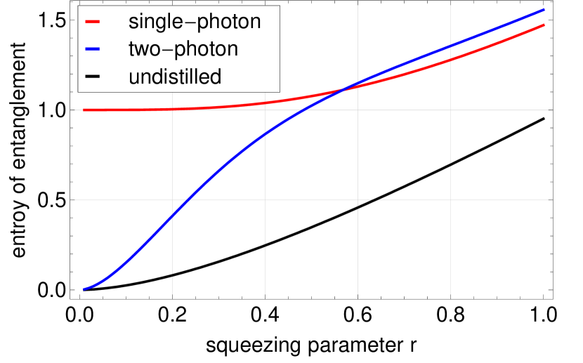
Figure 5: The entropy of entanglement for the single-photon subtracted states (red), the two-photon subtracted states (blue) and the undistilled states (black) as functions of the squeezing parameters $r$.

Let us denote the single-photon subtracted half-split squeezed vacuum as $\left|\Psi_{1}\right\rangle$.

$$\left|\Psi_{1}\right\rangle =\frac{1}{\sqrt{\mathcal{N}_{1}}}\hat{a}_{A}\left|\Psi_{0}\right\rangle,$$ (19)

$$\mathcal{N}_{1} =\frac{\sinh^{2}{r}}{2}.$$ (20)

From the argument in the last section, we have

$$\hat{S}_{A}(-r/2)\hat{S}_{B}(-r/2)\left|\Psi_{1}\right\rangle$$

$$=\frac{1}{\sqrt{\mathcal{N}_{1}}}\hat{S}_{A}(-r/2)\hat{S}_{B}(-r/2)\hat{a}_{A}\left|\Psi_{0}\right\rangle$$ (21)

$$=\frac{1}{\sqrt{\mathcal{N}_{1}}}(\hat{a}_{A}\cosh(r/2)+\hat{a}^{\dagger}_{A}\sinh(r/2))$$

$$\qquad\qquad\times\hat{S}_{A}(-r/2)\hat{S}_{B}(-r/2)\left|\Psi_{0}\right\rangle$$ (22)

$$=\frac{1}{\sqrt{\mathcal{N}_{1}}}(\hat{a}_{A}\cosh(r/2)+\hat{a}^{\dagger}_{A}\sinh(r/2))(1-\lambda^{\prime 2})^{\frac{1}{2}}$$

$$\qquad\qquad\times\sum_{n=0}^{\infty}\lambda^{\prime\,n}\left|n\right\rangle_{A}\left|n\right\rangle_{B}$$ (23)

$$=\frac{(1-\lambda^{\prime 2})^{\frac{1}{2}}}{\sqrt{\mathcal{N}_{1}}}\sum_{n=0}^{\infty}\lambda^{\prime\,n}(\cosh(r/2)\sqrt{n}\left|n-1\right\rangle_{A}$$

$$\qquad\qquad+\sinh(r/2)\sqrt{n+1}\left|n+1\right\rangle_{A})\left|n\right\rangle_{B}$$ (24)

$$=\frac{(1-\lambda^{\prime 2})^{\frac{1}{2}}}{\sqrt{\mathcal{N}_{1}}}\sum_{m=0}^{\infty}\sum_{n=0}^{\infty}A_{mn}\left|m\right\rangle_{A}\left|n\right\rangle_{B},$$ (25)

where

$$A_{mn} =\lambda^{\prime\,n}(\cosh(r/2)\sqrt{n}\delta_{m,n-1}$$

$$\qquad+\sinh(r/2)\sqrt{n+1}\delta_{m,n+1}).$$ (26)

From the singular values of matrix $A_{mn}$ (let them be $\alpha_{n}$), the Schmidt coefficients for $\left|\Psi_{1}\right\rangle$ are given by

$$c^{(1)}_{n}=\frac{(1-\lambda^{\prime 2})}{\mathcal{N}_{1}}\alpha_{n}^{2}.$$ (27)

Similar to the single photon case, we obtain a representation of the two-photon subtracted half-split squeezed vacuum $\left|\Psi_{2}\right\rangle$ in the following form.

$$\hat{S}_{A}(-r/2)\hat{S}_{B}(-r/2)\left|\Psi_{2}\right\rangle$$

$$=\frac{1}{\sqrt{N}_{2}}\hat{S}_{A}(-r/2)\hat{S}_{B}(-r/2)\hat{a}_{A}\hat{a}_{B}\left|\Psi_{0}\right\rangle$$ (28)

$$=\frac{(1-\lambda^{\prime 2})}{\sqrt{N}_{2}}\sum_{m=0}^{\infty}\sum_{n=0}^{\infty}B_{mn}\left|m\right\rangle_{A}\left|n\right\rangle_{B},$$ (29)

where

$$\mathcal{N}_{2} =\frac{2\sinh^{4}{r}+\cosh^{2}{r}\sinh^{2}{r}}{4}$$ (30)

$$B_{mn} =\cosh^{2}(r/2)(m+1)\lambda^{\prime\,m+1}\delta_{m,n}$$

$$+\sinh^{2}(r/2)m\lambda^{\prime\,m-1}\delta_{m,n}$$

$$+\cosh(r/2)\sinh(r/2)\sqrt{(m+1)(m+2)}\lambda^{\prime\,m+1}\delta_{m+2,n}$$

$$+\cosh(r/2)\sinh(r/2)\sqrt{m(m-1)}\lambda^{\prime\,m-1}\delta_{m-2,n}$$ (31)

Then the Schmidt coefficients $c^{(2)}_{n}$ for $\left|\Psi_{2}\right\rangle$ are given by the singular values $\beta_{n}$ of matrix $B_{mn}$:

$$c^{(2)}_{n} =\frac{(1-\lambda^{\prime 2})}{\mathcal{N}_{2}}\beta_{n}^{2}$$ (32)

(18), (27), (32) and (17) we can readily calculate the entropy of entanglement for those states. Fig. 5 shows the entropy of entanglement for the single-photon subtracted states $\left|\Psi_{1}\right\rangle$, the two-photon subtracted states $\left|\Psi_{2}\right\rangle$ and the undistilled states $\left|\Psi_{0}\right\rangle$ as functions of squeezing parameter $r$. Note that in an actual experiment, we have several experimental imperfections and we end up with a mixed state output. In such cases, the pure state descriptions above no longer hold and the entropy of entanglement is not a good measure of entanglement, but Fig. 5 still outlines the general behavior of this protocol.

Appendix B Calculating the logarithmic negativity

In principle, the logarithmic negativity $E_{\mathcal{N}}$ can be directly calculated when we know the 2-mode entangled state, as the sum of the negative eigenvalues of the partially transposed density matrix, $(\rho_{AB})^{T_{A}}$ Vidal and Werner (2002). In the experiment, however, we found that $E_{\mathcal{N}}$ is very sensitive to statistical noise in the measurements. Smaller data sets lead to larger errors in the reconstructed density matrix elements which ultimately leads to larger calculated $E_{\mathcal{N}}$ values. The intuitive understanding of this effect is the following: The absolute errors on each density matrix element due to statistical measurement noise are roughly the same. Hence, the relative errors are large for the high-photon number elements which are all close to zero - most likely their absolute values will increase due to the errors. But high photon numbers contribute a significant amount to the overall entanglement of the state, so in the end more noise will give seemingly higher entanglement.

We found empirically that the calculated negativity scales with the total data sample size $N$ as $E_{\mathcal{N}}(N)=a+b/\sqrt{N}$. We interpret this as $E_{\mathcal{N}}(\infty)=a$ being the “true” value that we would obtain in the asymptotic limit of very large data sample size, while the second term is the contribution from statistical noise. To obtain this value $E_{\mathcal{N}}(\infty)$ from a given data set of $N_{\mathrm{full}}$ samples, we perform multiple state reconstructions based on truncations of the full data set. Specifically, we partition the full set into $d$ subsets of $N_{d}\simeq N_{\mathrm{full}}/d$ samples each (with equal representation of all phase angles). The logarithmic negativity is then calculated from the reconstruction of all $d$ subsets, and we take the mean value of these to be an estimate for $E_{\mathcal{N}}(N_{d})$. We repeat the process for other numbers of partitions, $d$, and thereby get a plot as in Fig. 6 of the dependency of calculated entanglement on data sample size. A least-squares fit to $a+b/\sqrt{N}$ then gives us the asymptotic estimate $E_{\mathcal{N}}(\infty)$. We have confirmed by simulated data that this approach does in fact give the correct value for $E_{\mathcal{N}}$ within roughly $\pm 2\%$.

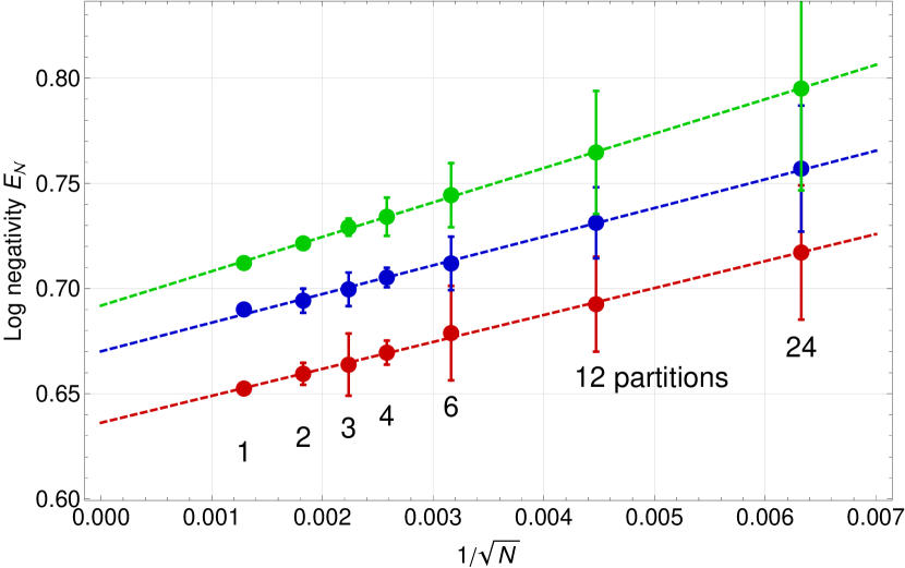
Figure 6: Estimation of the logarithmic negativity for infinitely many data samples. Each point shows the average and standard deviation of the calculated logarithmic negativities, $E_{\mathcal{N}}(N_{d})$ (average taken over the $d$ subsets of the full data set), versus $1/\sqrt{N_{d}}$, where $N_{d}$ is the size of each subset. The points are well fitted by a line whose y-axis intersection (infinite data size) gives a good estimate for the true $E_{\mathcal{N}}$ value (as confirmed by simulated data). The three plot series are from single-photon subtracted data sets with different initial squeezing levels, 2.3 (red), 3.2 (blue), and 4.2 (green) dB respectively.

References

- Briegel et al. (1998) H.-J. Briegel, W. Dür, J. I. Cirac, and P. Zoller, Phys. Rev. Lett. 81, 5932 (1998).
- Braunstein and van Loock (2005) S. L. Braunstein and P. van Loock, Rev. Mod. Phys. 77, 513 (2005).
- Eisert et al. (2002) J. Eisert, S. Scheel, and M. B. Plenio, Phys. Rev. Lett. 89, 137903 (2002).
- Fiurášek (2002) J. Fiurášek, Phys. Rev. Lett. 89, 137904 (2002).
- Giedke and Cirac (2002) G. Giedke and J. I. Cirac, Phys. Rev. A 66, 032316 (2002).
- Opatrný et al. (2000) T. Opatrný, G. Kurizki, and D.-G. Welsch, Phys. Rev. A 61, 032302 (2000).
- García-Patrón et al. (2004) R. García-Patrón, J. Fiurášek, N. J. Cerf, J. Wenger, R. Tualle-Brouri, and P. Grangier, Phys. Rev. Lett. 93, 130409 (2004).
- Bennett et al. (1996) C. H. Bennett, G. Brassard, S. Popescu, B. Schumacher, J. A. Smolin, and W. K. Wootters, Phys. Rev. Lett. 76, 722 (1996).
- Kwiat et al. (2001) P. G. Kwiat, S. Barraza-Lopez, A. Stefanov, and N. Gisin, Nature 409, 1014 (2001).
- Pan et al. (2001) J.-W. Pan, C. Simon, Č. Brukner, and A. Zeilinger, Nature 410, 1067 (2001).
- Yamamoto et al. (2003) T. Yamamoto, M. Koashi, Ş. K. Özdemir, and N. Imoto, Nature 421, 343 (2003).
- Reichle et al. (2006) R. Reichle, D. Leibfried, E. Knill, J. Britton, R. B. Blakestad, J. D. Jost, C. Langer, R. Ozeri, S. Seidelin, and D. J. Wineland, Nature (London) 443, 838 (2006).
- Ferraro et al. (2005) A. Ferraro, S. Olivares, and M. G. A. Paris, ArXiv Quantum Physics e-prints (2005), eprint arXiv:quant-ph/0503237.
- Hage et al. (2008) B. Hage, A. Samblowski, J. Diguglielmo, A. Franzen, J. Fiurášek, and R. Schnabel, Nature Phys. 4, 915 (2008).
- Dong et al. (2008) R. Dong, M. Lassen, J. Heersink, C. Marquardt, R. Filip, G. Leuchs, and U. L. Andersen, Nature Phys. 4, 919 (2008).
- Bartlett et al. (2002) S. D. Bartlett, B. C. Sanders, S. L. Braunstein, and K. Nemoto, Phys. Rev. Lett. 88, 097904 (2002).
- Ourjoumtsev et al. (2006) A. Ourjoumtsev, R. Tualle-Brouri, J. Laurat, and P. Grangier, Science 312, 83 (2006).
- Neergaard-Nielsen et al. (2006) J. S. Neergaard-Nielsen, B. Melholt Nielsen, C. Hettich, K. Mølmer, and E. S. Polzik, Phys. Rev. Lett. 97, 083604 (2006).
- Wakui et al. (2007) K. Wakui, H. Takahashi, A. Furusawa, and M. Sasaki, Opt. Express 15, 3568 (2007).
- Ourjoumtsev et al. (2007) A. Ourjoumtsev, A. Dantan, R. Tualle-Brouri, and P. Grangier, Phys. Rev. Lett. 98, 030502 (2007).
- Ourjoumtsev et al. (2009) A. Ourjoumtsev, F. Ferreyrol, R. Tualle-Brouri, and P. Grangier, Nature Phys. 5, 189 (2009).
- Takahashi et al. (2008) H. Takahashi, K. Wakui, S. Suzuki, M. Takeoka, K. Hayasaka, A. Furusawa, and M. Sasaki, Phys. Rev. Lett. 101, 233605 (2008).
- Lvovsky (2004) A. I. Lvovsky, J. Opt. B: Quantum Semiclass. Opt. 6, 556 (2004).
- Vidal and Werner (2002) G. Vidal and R. F. Werner, Phys. Rev. A 65, 032314 (2002).
- Eisert et al. (2004) J. Eisert, D. Brown, S. Scheel, and M. B. Plenio, Ann. Phys. (N.Y.) 311, 431 (2004).