Relativistic Stern-Gerlach Interaction in an RF Cavity

Abstract

The general expression of the Stern-Gerlach force is deduced for a relativistic charged spin-$\frac{1}{2}$ particle which travels inside a time varying magnetic field. This result was obtained either by means of two Lorentz boosts or starting from Dirac’s equation. Then, the utilization of this interaction for attaining the spin states separation is reconsidered in a new example using a new radio-frequency arrangement.

1 The Relativistic Stern-Gerlach Force

The time varying Stern-Gerlach, SG, interaction of a relativistic fermion with an e.m. wave has been proposed to separate beams of particles with opposite spin states corresponding to different energies[1]. We will show how spin polarized particle will exchange energy with the electromagnetic field of an RF resonator.

Let us denote with $(x,y,z)$ the coordinates of a particle in the laboratory, and with $(x^{\prime},y^{\prime},z^{\prime})$ the coordinates in the particle rest frame, PRF. In the latter the SG force that represents the action of an inhomogeneous magnetic field on a particle endowed with a magnetic moment $\vec{\mu}$ is

$$\textstyle\vec{f}^{\prime}_{SG}=\nabla^{\prime}(\vec{\mu}^{*}\cdot\vec{B}^{\prime})={\partial\over\partial x^{\prime}}(\vec{\mu}^{*}\cdot\vec{B}^{\prime}){\hat{x}}+{\partial\over\partial y^{\prime}}(\vec{\mu}^{*}\cdot\vec{B}^{\prime}){\hat{y}}+{\partial\over\partial z^{\prime}}(\vec{\mu}^{*}\cdot\vec{B}^{\prime}){\hat{z}}$$ (1)

with

$$\textstyle\vec{\mu}=g{e\over 2m}\vec{S}.$$ (2)

Here $e$ is the elementary charge with $``+"$ for protons and positrons, $p,e^{+}$, and ${}^{\prime\prime}=^{\prime\prime}$ for antiprotons and electrons, $\bar{p},e^{-}$, making $\vec{\mu}$ and $\vec{S}$ either parallel or antiparallel to each other, respectively. $m$ is the rest mass of the particle, $g$ the gyromagnetic ratio and $a$ the anomaly defined as

$$\textstyle a={{g-2}\over 2}=\left\{\begin{array}[]{ll}1.793~{}(g=5.586)&{\mathrm{for}}~{}p,\bar{p}\\ \\ 1.160\times 10^{-3}&{\mathrm{for}}~{}e^{\pm}\end{array}\right..$$ (3)

Notice that in Eq.(1) we have defined the magnetic moment as $\mu^{*}$ in the rest frame, rather than as $\mu^{\prime}$. In the rest frame the quantum vector $\vec{S}$, or spin, has modulus $|\vec{S}|=\sqrt{s(s+1)}{\hbar}$ and its component parallel to the magnetic field lines can only take the following values

$$\textstyle S_{m}=(-s,~{}-s+1,....,s-1,~{}s)\hbar,$$ (4)

where $\hbar$ is the reduced Planck’s constant. Combining Eqs.(2) and (4) we obtain for the magnetic moment in the PRF

$$\textstyle\mu=|\vec{\mu}|=g{|e|\hbar\over 4m}=\left\{\begin{array}[]{l}1.41\times 10^{-26}~{}JT^{-1}\\ \\ 9.28\times 10^{-24}~{}JT^{-1}\end{array}\right..$$ (5)

For a particle traveling along the axis $\hat{z}$, the Lorentz transformations of the differential operators and of the force yield

$$\textstyle\left\{\begin{array}[]{lll}{\partial\over\partial x^{\prime}}={\partial\over\partial x}&{\partial\over\partial y^{\prime}}={\partial\over\partial y}&{\partial\over\partial z^{\prime}}=\gamma\,\left({\partial\over\partial z}+{\beta\over c}{\partial\over\partial t}\right)\\ \\ \vec{f}_{\perp}={1\over\gamma}\,\vec{f}^{\prime}_{\perp}&\vec{f}_{\parallel}=\vec{f}^{\prime}_{\parallel}&(f_{z}=f^{\prime}_{z})\end{array}\right..$$ (6)

The force (1) is boosted to the laboratory system as

$$\textstyle\vec{f}_{SG}={1\over\gamma}{\partial\over\partial x}(\vec{\mu}^{*}\cdot\vec{B}^{\prime}){\hat{x}}+{1\over\gamma}{\partial\over\partial y}(\vec{\mu}^{*}\cdot\vec{B}^{\prime}){\hat{y}}+{\partial\over\partial z^{\prime}}(\vec{\mu}^{*}\cdot\vec{B}^{\prime}){\hat{z}}.$$ (7)

Because of the Lorentz transformation of the fields[3] $\vec{E},\vec{B}$ and $\vec{E}^{\prime},\vec{B}^{\prime}$

$$\textstyle\left\{\begin{array}[]{l}\vec{E}^{\prime}=\gamma(\vec{E}+c\vec{\beta}\times\vec{B})-{\gamma^{2}\over\gamma+1}\vec{\beta}(\vec{\beta}\cdot\vec{E})\\ \\ \vec{B}^{\prime}=\gamma\left(\vec{B}-{\vec{\beta}\over c}\times\vec{E}\right)-{\gamma^{2}\over\gamma+1}\vec{\beta}(\vec{\beta}\cdot\vec{B})\end{array}\right..$$ (8)

the energy in the rest frame $(\vec{\mu}^{*}\cdot\vec{B}^{\prime})$ becomes

$$\textstyle(\vec{\mu}^{*}\cdot\vec{B}^{\prime})=\gamma\mu^{*}_{x}\left(B_{x}+{\beta\over c}E_{y}\right)+\gamma\mu^{*}_{y}\left(B_{y}-{\beta\over c}E_{x}\right)+\mu^{*}_{z}B_{z}.$$ (9)

Combining Eqs.(9) and (7), by virtue of Eq.(6), after some algebra we can finally obtain the SG force components in the laboratory frame:

$$\left\{\begin{array}[]{l}f_{x}=\mu^{*}_{x}\left({\partial B_{x}\over\partial x}+{\beta\over c}{\partial E_{y}\over\partial x}\right)+\mu^{*}_{y}\left({\partial B_{y}\over\partial x}-{\beta\over c}{\partial E_{x}\over\partial x}\right)+{1\over\gamma}\mu^{*}_{z}{\partial B_{z}\over\partial x}\\ \\ f_{y}=\mu^{*}_{x}\left({\partial B_{x}\over\partial y}+{\beta\over c}{\partial E_{y}\over\partial y}\right)+\mu^{*}_{y}\left({\partial B_{y}\over\partial y}-{\beta\over c}{\partial E_{x}\over\partial y}\right)+{1\over\gamma}\mu^{*}_{z}{\partial B_{z}\over\partial y}\\ \\ f_{z}=\mu^{*}_{x}C_{zx}+\mu^{*}_{y}C_{zy}+\mu^{*}_{z}C_{zz},\end{array}\right.$$ (10)

with

$$\textstyle\left\{\begin{array}[]{l}C_{zx}=\gamma^{2}\left[\left({\partial B_{x}\over\partial z}+{\beta\over c}{\partial B_{x}\over\partial t}\right)+{\beta\over c}\left({\partial E_{y}\over\partial z}+{\beta\over c}{\partial E_{y}\over\partial t}\right)\right]\\ \\ C_{zy}=\gamma^{2}\left[\left({\partial B_{y}\over\partial z}+{\beta\over c}{\partial B_{y}\over\partial t}\right)-{\beta\over c}\left({\partial E_{x}\over\partial z}+{\beta\over c}{\partial E_{x}\over\partial t}\right)\right]\\ \\ C_{zz}=\gamma\left({\partial B_{z}\over\partial z}+{\beta\over c}{\partial B_{z}\over\partial t}\right)\end{array}\right..$$ (11)

These results can also be obtained from the quantum relativistic theory of the spin-$\frac{1}{2}$ charged particle[2]. Let us introduce the Dirac Hamiltonian

$$\textstyle H=e\phi+c\vec{\alpha}\cdot(\vec{p}-e\vec{A})+\gamma_{0}mc^{2}$$ (12)

having made use of the Dirac’s matrices

$$\textstyle\vec{\gamma}=\left(\matrix{\mathcal{O}&\vec{\sigma}\cr-\vec{\sigma}&\mathcal{O}\cr}\right),~{}~{}~{}\gamma_{0}=\left(\matrix{\mathcal{I}&\mathcal{O}\cr 0&-\mathcal{I}\cr}\right),~{}~{}~{}\vec{\alpha}=\gamma_{0}\vec{\gamma}=\left(\matrix{\mathcal{O}&\vec{\sigma}\cr\vec{\sigma}&\mathcal{O}\cr}\right),$$ (13)

where $\vec{\sigma}$ is a vector whose components are the Pauli’s matrices

$$\textstyle\sigma_{x}=\left(\matrix{0&-i\cr i&0\cr}\right),~{}~{}\sigma_{y}=\left(\matrix{1&0\cr 0&-1\cr}\right),~{}~{}\sigma_{z}=\left(\matrix{0&1\cr 1&0\cr}\right),~{}~{}$$ (14)

$\mathcal{I}$ is the $2\times 2$ identity matrix, $\mathcal{O}$ the null matrix and having chosen the $y$-axis parallel to the main magnetic field. A standard derivation leads to the non relativistic expression of the Hamiltonian exhibiting the SG interaction with the “normal” magnetic moment

$$\textstyle\tilde{H}=e\phi+\frac{1}{2m}(\vec{p}-e\vec{A})^{2}-\frac{e\hbar}{2m}(\vec{\sigma}\cdot\vec{B})$$ (15)

which coincides with the Pauli equation and is valid in the PRF.

To complete the derivation we must add the contribution from the anomalous magnetic moment to the SG energy term in the previous equation, with a factor $1+a=\frac{g}{2}$, yielding

$$\textstyle-\frac{g}{2}\frac{e\hbar}{2m}\;\vec{\sigma}\cdot\vec{B}=-\vec{\mu}^{*}\cdot\vec{B}~{}~{}~{}~{}{\mathrm{with}}~{}~{}~{}~{}\vec{\mu}^{*}=g\frac{e\hbar}{4m}\vec{\sigma}.$$ (16)

In order to obtain the $z$-component of the SG force in the Laboratory frame along the direction of motion of the particle, we must boost the whole Pauli term of Eq.(15) by using the unitary operator $U$ in the Hilbert space[4], which expresses the Lorentz transformation

$$\textstyle U^{-1}\left[g\frac{e\hbar}{4m}(\gamma_{0}\vec{\sigma}\cdot\vec{B}^{\prime})\right]U=g\frac{e\hbar}{4m}(\gamma_{0}\vec{\sigma}\cdot\vec{B}^{\prime})\left[S^{-1}(\gamma_{0}\sigma_{x})S+S^{-1}(\gamma_{0}\sigma_{y})S+S^{-1}(\gamma_{0}\sigma_{z})S\right]$$ (17)

that can be written in terms of the equivalent transformation in the $4\times 4$ spinor space

$$\textstyle S=\exp{\left\{\gamma_{0}(\vec{\gamma}\cdot\hat{v})\frac{u}{2}\right\}}=\cosh{\frac{u}{2}}+\left(\matrix{0&\sigma_{z}\cr\sigma_{z}&0\cr}\right)\sinh{\frac{u}{2}}$$ (18)

with

$$\textstyle\hat{v}=\frac{\vec{v}}{|\vec{v}|},~{}~{}\cosh u=\frac{1}{\sqrt{1-\beta^{2}}}=\gamma={\mathrm{Lorentz~{}factor}},~{}~{}\sinh u=\sqrt{\gamma^{2}-1}~{}~{}~{}\left(\beta=\frac{v}{c}\right).$$ (19)

From Eqs.(17) and (18), due to the algebraic structure of the $\gamma$ and $\sigma$ matrices, we obtain in the laboratory frame the three components of the SG force

$$\left\{\begin{array}[]{lll}S^{-1}(\gamma_{0}\sigma_{x})S&=&\gamma_{0}\sigma_{x}\\ S^{-1}(\gamma_{0}\sigma_{y})S&=&\gamma_{0}\sigma_{y}\\ S^{-1}(\gamma_{0}\sigma_{z})S&=&\gamma(\gamma_{0}\sigma_{z})+i\gamma_{0}\gamma_{5}\sqrt{\gamma^{2}-1}\end{array}\right.,$$ (20)

with

$$\textstyle\gamma_{5}=\gamma_{x}\gamma_{y}\gamma_{z}\gamma_{0}=i\left(\matrix{\mathcal{O}&\mathcal{I}\cr\mathcal{I}&\mathcal{O}}\right).$$ (21)

From Eqs.(20) we can deduce the expectation values of the SG force in the Laboratory system with a defined spin -along the $y$-axis in our case- via the expectation values of the Pauli matrices and of the Pauli interaction term of the proper force

$$\textstyle f_{z}=\gamma_{0}\sigma_{y}\gamma^{2}\mu^{*}\left[\left(\frac{\partial B_{y}}{\partial z}+\frac{\beta}{c}\frac{\partial B_{y}}{\partial t}\right)-\frac{\beta}{c}\left(\frac{\partial E_{x}}{\partial z}+\frac{\beta}{c}\frac{\partial E_{x}}{\partial t}\right)\right].$$ (22)

In our case only the second of Eqs.(20) gives a non vanishing result, while both the first and third produce a null contribution to the force, because of the orthogonality of the two spin states $s=\pm\frac{1}{2}$ and the properties of the $\sigma$ matrices.

2 The radio-frequency system

Let us consider the standing waves built up inside a rectangular radio-frequency resonator, tuned to a generic TE Mode[1]. Resonator dimensions are: width $a$, height $b$ and length $d$, as shown in Fig.1. On the cavity axis, which coincides with the beam axis, the electric and magnetic fields are[5]

$$\begin{array}[]{lcl}E_{x}&=&-B_{0}\left({n\pi\over b}\right){\omega\over K_{c}^{2}}\cos\left({m\pi x\over a}\right)\sin\left({n\pi y\over b}\right)\sin\left({p\pi z\over d}\right)\sin\,\omega t\\ \\ E_{y}&=&B_{0}\left({m\pi\over a}\right){\omega\over K_{c}^{2}}\sin\left({m\pi x\over a}\right)\cos\left({n\pi y\over b}\right)\sin\left({p\pi z\over d}\right)\sin\,\omega t\\ \\ E_{z}&=&0~{}~{}~{}~{}~{}~{}~{}~{}~{}~{}~{}~{}[{\mathrm{as~{}typical~{}for~{}any~{}TE~{}mode}}]\\ \\ B_{x}&=&-{B_{0}\over K_{c}^{2}}\left({m\pi\over a}\right)\left({p\pi\over d}\right)\sin\left({m\pi x\over a}\right)\cos\left({n\pi y\over b}\right)\cos\left({p\pi z\over d}\right)\cos\,\omega t\\ \\ B_{y}&=&-{B_{0}\over K_{c}^{2}}\left({n\pi\over b}\right)\left({p\pi\over d}\right)\cos\left({m\pi x\over a}\right)\sin\left({n\pi y\over b}\right)\cos\left({p\pi z\over d}\right)\cos\,\omega t\\ \\ B_{z}&=&B_{0}\cos\left({m\pi x\over a}\right)\cos\left({n\pi y\over b}\right)\sin\left({p\pi z\over d}\right)\cos\,\omega t\end{array}$$

where $B_{0}$ is the RF peak magnetic field, $m$, $n$ and $p$ are integer mode indeces, and

$$\textstyle K_{c}=\sqrt{\left({m\pi\over a}\right)^{2}+\left({n\pi\over b}\right)^{2}}.$$ (23)

The angular frequency of the e.m. wave from the RF generator is

$$\textstyle\omega=\omega_{\mathrm{RF}}={{2\pi c}\over\lambda_{\mathrm{RF}}}=c\sqrt{\left({m\pi\over a}\right)^{2}+\left({n\pi\over b}\right)^{2}+\left({p\pi\over d}\right)^{2}}.$$ (24)

In contrast with an open waveguide, in a bounded cavity we can define a phase velocity $V_{\mathrm{ph}}$ and a cavity wavelength $\lambda_{\mathrm{wg}}$, as typical of any e.m. in a refractive media, according to the relations

$$\textstyle\frac{V_{\mathrm{ph}}}{c}=\beta_{\mathrm{ph}}={d\over p\pi}\sqrt{\left({m\pi\over a}\right)^{2}+\left({n\pi\over b}\right)^{2}+\left({p\pi\over d}\right)^{2}}.$$ (25)

and

$$\textstyle\lambda_{\mathrm{wg}}=\beta_{\mathrm{p}h}\lambda_{\mathrm{RF}}.$$ (26)

It is also

$${V_{\mathrm{ph}}}=\beta_{\mathrm{ph}}c=\beta_{\mathrm{ph}}\frac{\lambda_{\mathrm{R}F}}{\tau_{\mathrm{R}F}}=\frac{\lambda_{\mathrm{w}g}}{\tau_{\mathrm{R}F}}$$ (27)

Notice that $\beta_{\mathrm{ph}}$ can take any value, even larger than one, since it is freely dependent on the cavity geometrical parameters. Moreover, combining Eqs.(24) and (25) we obtain

$$\textstyle d=\frac{1}{2}p\beta_{\mathrm{ph}}\lambda_{\mathrm{RF}}=\frac{1}{2}p\lambda_{\mathrm{wg}}$$ (28)

Figure 1: Sketch of the rectangular cavity. The coordinates of the beam axis are $x=\frac{a}{2}$ and $y=\frac{b}{2}$.

which describes the connection between the cavity length $d$ and the wavelengths, as shown in Fig.2.

Figure 2: Vertical component (inside the cavity) and fringes (at both cavity ends) of $B_{y}$ for $p=1$.

For simplicity, let’s choose the transverse electric mode ${\mathrm{TE}}_{01p}$, so Eqs.(24) and (25) reduce respectively to

$$\textstyle\omega=\omega_{\mathrm{RF}}=c\sqrt{\left(\frac{\pi}{b}\right)^{2}+\left(\frac{p\pi}{d}\right)^{2}}=\beta_{\mathrm{ph}}c\frac{\pi}{d}~{}~{}~{}~{}{\mathrm{and}}~{}~{}~{}~{}\beta_{\mathrm{ph}}=\sqrt{1+\left(\frac{pd}{b}\right)^{2}}$$ (29)

or, setting the mode index $p=1$,

$$\textstyle\omega=\omega_{\mathrm{RF}}=c\sqrt{\left(\frac{\pi}{b}\right)^{2}+\left(\frac{\pi}{d}\right)^{2}}=\beta_{\mathrm{ph}}c\frac{\pi}{d}~{}~{}~{}~{}{\mathrm{and}}~{}~{}~{}~{}\beta_{\mathrm{ph}}=\sqrt{1+\left(\frac{d}{b}\right)^{2}},$$ (30)

which are the quantities pertaining to the preferred ${\mathrm{TE}}_{011}$ mode whose non zero field components on the cavity axis are

$$\textstyle\left\{\begin{array}[]{l}B_{y}(z,t)=-B_{0}\frac{b}{d}\cos\left(\frac{\pi z}{d}\right)\cos\omega t\\ \\ E_{x}(z,t)=-\omega B_{0}\frac{b}{\pi}\sin\left(\frac{\pi z}{d}\right)\sin\omega t\end{array}\right..$$ (31)

It is important to emphasize that in all the field components met so far there is a clear separation between spatial and temporal contributions, as typical of standing waves. Besides, the boundary conditions of the electric and magnetic fields of the e.m. dictate the shape of the spatial component which, in turn, oscillates in time with the frequency $\omega_{RF}$. Then, at the cavity entrance and exit the field components  (31) become on axis

$$\textstyle{\mathrm{Entrance}}\Longrightarrow\left\{\begin{array}[]{l}B_{y}(0,t)=-B_{0}\frac{b}{d}\cos\omega t\\ \\ E_{x}(0,t)=0\end{array}\right..$$ (32)

and

$$\textstyle{\mathrm{Exit}}\Longrightarrow\left\{\begin{array}[]{l}B_{y}(d,t)=-B_{0}\frac{b}{d}\cos\pi\cos\omega t=B_{0}\frac{b}{d}\cos\omega t\\ \\ E_{x}(d,t)=-\omega\frac{b}{\pi}\sin\pi\sin\omega t=0\end{array}\right..$$ (33)

where $t$ is a generic time. The null values of $E_{x}$ at the cavity ends confirm a typical pattern of the transverse electric mode.

3 Stern-Gerlach interaction with the cavity field

From Eq.(22), after some algebra, we obtain tha a charged fermion which crosses a radio-frequency resonator, tuned on the TE₀₁₁ mode, acquires (or loses) an energy amount when interacts with the field component in the “body” of the cavity shown in Fig. 2[1]

$$(\delta U)_{\mathrm{X-ing}}=\int_{0}^{d}\,f_{z}dz=\int_{0}^{d}\,\mu^{*}C_{zy}dz=\beta^{2}\gamma^{2}B_{0}\mu^{*}\frac{b}{d}\frac{\beta_{\mathrm{ph}}^{2}(2-\beta^{2})-1}{\beta_{\mathrm{ph}}^{2}-\beta^{2}}\left(1+\cos\frac{\beta_{\mathrm{ph}}}{\beta}\pi\right)$$ (34)

still assuming that the spin is not precessing.

However, since the cavity cannot be completely enclosed but must have apertures at both ends to allow the particle bean to pass through and consequently will have fringe fields, in order to calculate the full SG interaction it is necessary to deal with the interaction with these fields. This is discussed right below.

3.1 Fringe fields

In order to fulfill the boundary conditions (32) and (33), a cavity tuned in its ${\mathrm{TE}}_{011}$ mode must be exactly filled by either an even or an odd number of cavity dependent half wave-lengths, Eq.(26), as illustrated in Figs. 2 and 3.

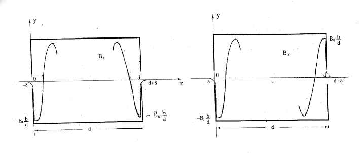
Figure 3: Edge fields at both ends of a single cavity for $p$ equal to either an even number (left) or an odd number (right).

Consider now a bunch of particles crossing the cavity in synchronism with the RF field. This requires that the bunch centre of mass that enters the cavity at the instant $t=0$ and would leave the cavity at $t=\tau_{\mathrm{RF}}$, at magnetic field values, respectively

$$\textstyle B_{y}(0,0)=-B_{0}\frac{b}{d}~{}~{}~{}~{}{\mathrm{and}}~{}~{}~{}~{}B_{y}(d,\tau_{\mathrm{RF}})=B_{0}\frac{b}{d}$$ (35)

The field values at both ends fade rapidly to zero over a small distance $|\delta|$ just outside the cavity (see Figures.) We may consider these fringe fields as small-valued functions in the $(y,z)$-plane, since the time $\delta t$ necessary for a particle to proceed through this distances can be very small in comparison with $\tau_{\mathrm{RF}}$, depending of course by the size of the beam channel, or

$$\textstyle\left\{\begin{array}[]{llllll}\left[B_{y}\right]_{\mathrm{in}}&=&-B_{0}\frac{b}{d}\;g(z)&{\mathrm{with}}&g(-\delta)=0,&g(0)=1\\ \\ \left[B_{y}\right]_{\mathrm{out}}&=&B_{0}\frac{b}{d}\;h(z)&{\mathrm{with}}&h(d)=1,&h(d+\delta)=0\end{array}\right..$$ (36)

Under these conditions, a relativistic fermion with its spin directed along the $y$-axis and traversing the cavity will experience a SG force parallel to the $z$-axis (direction of motion), see Eq.(10)

$$\textstyle f_{z}=\mu^{*}C_{zy}$$ (37)

where $C_{zy}$ is given by the second of the set of Eqs.(11). For the moment we assume that the spin will conserve its orientation during traversal

The electric field $E_{x}$ and its derivatives in this equation are almost constantly zero, because of the boundary conditions on the walls of the cavity and at the extreme points $z=-\delta$ and $z=d+\delta$. Furthermore, the function$\left(\frac{\partial B_{y}}{\partial t}\right)$ is almost zero along the fringe segments because of its proportionality to $\sin\omega t$, with $t$ equal to the $\delta t$ mentioned before. Consequently we have

$$\textstyle C_{zy}\simeq\gamma^{2}\frac{\partial B_{y}}{\partial z},$$ (38)

and for the entire fringe field

$$\textstyle\left\{\begin{array}[]{lll}\left[f_{z}\right]_{\mathrm{in}}&=&-B_{0}\mu^{*}\frac{b}{d}\gamma^{2}\left(\frac{dg(z)}{dz}\right)\\ \\ \left[f_{z}\right]_{\mathrm{out}}&=&B_{0}\mu^{*}\frac{b}{d}\gamma^{2}\left(\frac{dh(z)}{dz}\right)\end{array}\right..$$ (39)

Making use of eqs. (38) and (39), the energy increments $[\delta U]_{\mathrm{i}n}$ and $[\delta U]_{\mathrm{o}ut}$ related to the fringe fields are easily evaluated since the integrals $\int_{-\delta}^{0}f_{z}dz$ and $\int_{d}^{d+\delta}f_{z}dz$ only depend upon the extreme points (36) and do not depend on the curve that connects them. In fact $f_{z}dz$ becomes an exact differential. Then we obtain for the energy exchange at both edges

$$\textstyle(\delta U)_{\mathrm{in}}=(\delta U)_{\mathrm{out}}=-B_{0}\mu^{*}\frac{b}{d}\gamma^{2}.$$ (40)

The total energy exchange at the edges is therefore

$$\textstyle(\delta U)_{\mathrm{ff}}=(\delta U)_{\mathrm{in}}+(\delta U)_{\mathrm{out}}=-2B_{0}\mu^{*}\frac{b}{d}\gamma^{2}.$$ (41)

3.2 Full energy interaction

By adding the fringe contributions (41) to the cavity body crossing contribution (34) seen before, obtain

$$(\delta U)_{\mathrm{tot}}=(\delta U)_{\mathrm{ff}}+(\delta U)_{\mathrm{X}}=-\gamma^{2}B_{0}\mu^{*}\frac{b}{d}f(\beta_{\mathrm{ph}},\beta)$$ (42)

with

$$\textstyle f(\beta_{\mathrm{ph}},\beta)=\left[2-\beta^{2}\frac{\beta_{\mathrm{ph}}^{2}(2-\beta^{2})-1}{\beta_{\mathrm{ph}}^{2}-\beta^{2}}\left(1+\cos\frac{\beta_{\mathrm{ph}}}{\beta}\pi\right)\right].$$ (43)

For ultra relativistic particles ($\beta\simeq 1$) Eq. (42) reduces to

$$(\delta U)_{\mathrm{tot}}\simeq-\gamma^{2}B_{0}\mu^{*}\frac{b}{d}(1-\cos\beta_{\mathrm{ph}}\pi).$$ (44)

This last result deserves a few comments. In fact, if we set

$$\textstyle\beta_{\mathrm{ph}}=2~{}~{}~{}\Longrightarrow~{}~{}~{}d=\frac{1}{2}\lambda_{\mathrm{wg}}=\lambda_{\mathrm{RF}}$$ (45)

the total energy contribution (44) vanishes, implying a full cancellation of the effect.

On the other hand if we set

$$\textstyle\beta_{\mathrm{ph}}=3~{}~{}~{}\Longrightarrow~{}~{}~{}d=\frac{1}{2}\lambda_{\mathrm{wg}}=\frac{3}{2}\lambda_{\mathrm{RF}}$$ (46)

the total energy contribution (44) becomes

$$\textstyle(\delta U)_{\mathrm{tot}}\simeq-2\gamma^{2}B_{0}\mu^{*}\frac{b}{d}$$ (47)

as deduced from Eq.(28). In Table I we gather values calculated from Eq.(43) for non-relativistic and ultra-relativistic particles for, either $\beta_{\mathrm{ph}}=2$ or $\beta_{\mathrm{ph}}=3$ at two proton energies. Each $\beta_{\mathrm{ph}}$ is accompanied by the corresponding ratio cavity-length over cavity-height.

Table I: $f(\beta_{\mathrm{ph}},\beta)$

$\beta_{\mathrm{ph}}\Rightarrow\frac{d}{b}$	Low Energy	High Energy
	(e.g. $W_{\mathrm{kin}}$ = 5 MeV)	(e.g. $W_{\mathrm{kin}}$ = 30 GeV)
2 $\Rightarrow$ 1.732	2.01	0
3 $\Rightarrow$ 2.828	2.02	2

Furthermore, if we consider two contiguous cavities, there will be a gradient between the positive $B_{y}$ at the end of the first cavity and a negative $B_{y}$ at the beginning of the second cavity, as shown in Fig. 4. In this case we may consider the magnetic field at the interface as linearly dependent on $z$, that is

$$\textstyle[B_{y}(z)]_{\mathrm{X-ing}}=-2B_{0}\frac{b}{d\delta}z.$$ (48)

Reiterating what done before, obtain

$$\begin{array}[]{rcl}\frac{\partial}{\partial z}\left[B_{y}(z)\right]_{\mathrm{X-ing}}&=&-2B_{0}\frac{b}{d\delta}\\ \\ f_{z}&=&-2B_{0}\mu^{*}\frac{b}{d\delta}\gamma^{2}\\ \\ (\delta U)_{\mathrm{cav2cav}}=(\delta U)_{\mathrm{cc}}&=&\int_{-\frac{\delta}{2}}^{\frac{\delta}{2}}f_{z}dz=-2B_{0}\mu^{*}\frac{b}{d}\frac{1}{\delta}\left[\frac{\delta}{2}-\left(-\frac{\delta}{2}\right)\right]\gamma^{2}=-2B_{0}\mu^{*}\frac{b}{d}\gamma^{2}\end{array}$$ (49)

which means that, for $N$ cavities, we shall have as final result for ultra relativistic particles

$$\textstyle(\delta U)_{\mathrm{tot}}=N(\delta U)_{\mathrm{X-ing}}-(N-1)(\delta U)_{\mathrm{cc}}-(\delta U)_{\mathrm{ff}}=\left\{\begin{array}[]{ll}0&{\mathrm{for}}~{}\beta_{ph}=2\\ \\ \frac{2N}{2.83}B_{0}\mu^{*}\gamma^{2}&{\mathrm{for}}~{}\beta_{ph}=3\end{array}\right..$$ (50)

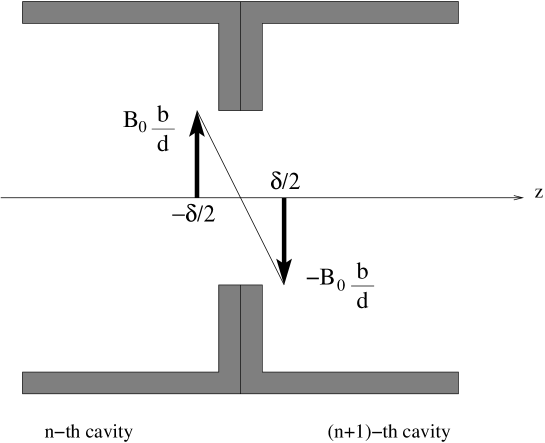
Figure 4: Magnetic field gradient between two contiguous cavities

Conversely, if $\beta_{\mathrm{ph}}$ is even, particles with their spin pointing always in the same direction cannot exchange energy with the standing wave of a TE resonator. A spin rotator[6] can align the particle magnetic moments either parallel or anti-parallel to the directions of the magnetic field gradients, thus allowing the desired energy interaction. This situation would be similar to what happens in a multi-stage tandem van de Graaff, where the ions are repetitively accelerated by the same electrostatic field, becoming alternatively negative, via an addition of electrons, or positive, via electron stripping.

Unfortunately, the field integral ($B_{\mathrm{M}}d=\beta\pi\frac{mc}{ae}=\beta\;5.46$ Tm, for $p,\bar{p}$) for attaining a spin rotation is so large that this solution is unpractical. Instead, the example of $\beta_{\mathrm{ph}}$ equal to an odd number seems much more suitable since does not require cumbersome magnets, but only longer cavities (compare Eqs. (45) and (46)). In fact, the magnetic moments are (de)accelerated by the field tails at the cavity ends, while don’t change their energy when crossing the cavities. This situation resembles the Wideroe linac where the charged particles are accelerated by the electric fields between two contiguous drift tubes, but don’t change their energy while crossing the tubes themselves.

4 Concluding remarks

On the basis of the previous estimates, we feel ready to propose the time varying SG interaction as a method for attaining a spin state separation of an unpolarized beam of, say (anti)protons, since the energy of particles with opposite spin orientations will differ and beams in the two states can be separated. In a first stage of the study of a sensible practical design, we intend to proceed with numerical simulations. As a first step, we intend to verify the correctness of Eqs.(42) and (43) setting once $\beta_{\mathrm{ph}}=2$ and then $\beta_{\mathrm{ph}}=3$, in a cavity where the field line pattern can be realistically controlled.

Beyond the verification of the present theory, there is also the aim of studying the effects generated by the spin precession inside the cavity, that we did not yet address in this note.

Next, we shall consider a spin splitter scheme based on the lattice of an existing or planned (anti)proton ring endowed with an array of splitting cavities. The principal aim of the latter implementations is to check the mixing effect[7][8] of the longitudinal phase-plane filamentation, i.e. the actual foe which could frustrate the entire spin splitting process.

5 Acknowledgments

First, we want to thank Waldo MacKay, who has participated on so many discussions on the whole idea but who was regrettably prevented by numerous commitments from participate to the editing of the present note. We thank Renzo Parodi for his help for us to better understand the subtleties of the standing waves building up. Thanks are also due to Chris Tschalaer for fruitful discussions on the role of the fringe fields.

References

• [1] M. Conte, M. Ferro, G. Gemme, W.W. MacKay, R. Parodi, M. Pusterla: The Stern-Gerlach Interaction Between a Traveling Particle and a Time Varying Magnetic Field, INFN/TC-00/03, 22 Marzo 2000. (http:xxx.lanl.gov/listphysics/0003, preprint 0003069)
• [2] P. Cameron, M. Conte, A. Luccio, W.W. MacKay, M. Palazzi and M. Pusterla: The Relativistic Stern-Gerlach Interaction and Quantum Mechanics Implications, Proceedings of the SPIN2002 Symposium, 9-14 September 2002, Brookhaven, Eds. Y.I. Makdisi, A.U. Luccio and W.W. MacKay, AIP Conference Proceedings 675 (2003) p. 786.
• [3] J.D.Jackson, Classical Elecrodynamics, John Wiley & Sons Inc., New York 1975
• [4] R.P. Feynman, Quantum Electrodynamics, W.A. Benjamin Inc., New York 1961.
• [5] S. Ramo, J.R. Whinnery and T. Van Duzer, Fields and Waves in Communication Electronics, John Wiley and & Sons, New York, 1965.
• [6] M.Conte,A.U.Luccio,W.W.MacKay and M.Pusterla Stern Gerlach Force on a Precessing Magnetic Moment Proc. PAC07, Albuquerque, NM (2007), p.3729
• [7] M. Conte, W.W. MacKay and R. Parodi: An Overview of the Longitudinal Stern-Gerlach Effect, BNL-52541, UC-414, November 17 1997.
• [8] M. Palazzi: Ph.D Thesis, Genoa University, June 6 2003.