Finite-size effects in film geometry with nonperiodic boundary conditions:
Gaussian model and renormalization-group theory at fixed dimension

Abstract

Finite-size effects are investigated in the Gaussian model with isotropic and anisotropic short-range interactions in film geometry with nonperiodic boundary conditions (b.c.) above, at, and below the bulk critical temperature $T_{\text{c}}$. We have obtained exact results for the free energy and the Casimir force for antiperiodic, Neumann, Dirichlet, and Neumann-Dirichlet mixed b.c. in $1<d<4$ dimensions. For the Casimir force, finite-size scaling is found to be valid for all b.c.. For the free energy, finite-size scaling is valid in $1<d<3$ and $3<d<4$ dimensions for antiperiodic, Neumann, and Dirichlet b.c., but logarithmic deviations from finite-size scaling exist in $d=3$ dimensions for Neumann and Dirichlet b.c.. This is explained in terms of the borderline dimension $d^{*}=3$, where the critical exponent $1-\alpha-\nu=(d-3)/2$ of the Gaussian surface energy density vanishes. For Neumann-Dirichlet b.c., finite-size scaling is strongly violated above $T_{\text{c}}$ for $1<d<4$ because of a cancelation of the leading scaling terms. For antiperiodic, Dirichlet, and Neumann-Dirichlet b.c., a finite film critical temperature $T_{\text{c,film}}(L)<T_{\text{c}}$ exists at finite film thickness $L$. Our results include an exact description of the dimensional crossover between the $d$-dimensional finite-size critical behavior near bulk $T_{\text{c}}$ and the $(d{-}1)$-dimensional critical behavior near $T_{\text{c,film}}(L)$. This dimensional crossover is illustrated for the critical behavior of the specific heat. Particular attention is paid to an appropriate representation of the free energy in the region $T_{\text{c,film}}(L)\leq T\leq T_{\text{c}}$. For $2<d<4$, the Gaussian results are renormalized and reformulated as one-loop contributions of the $\varphi^{4}$ field theory at fixed dimension $d$ and are then compared with the $\varepsilon=4-d$ expansion results at $\varepsilon=1$ as well as with $d=3$ Monte Carlo data. For $d=2$, the Gaussian results for the Casimir force scaling function are compared with those for the Ising model with periodic, antiperiodic, and free b.c.; unexpected exact relations are found between the Gaussian and Ising scaling functions. For both the $d$-dimensional Gaussian model and the two-dimensional Ising model it is shown that anisotropic couplings imply nonuniversal scaling functions of the Casimir force that depend explicitly on microscopic couplings. Our Gaussian results provide the basis for the investigation of finite-size effects of the mean spherical model in film geometry with nonperiodic b.c. above, at, and below the bulk critical temperature.

I Introduction and Summary

Critical phenomena in confined systems have remained an important topic of research over the past decades. Much interest has been devoted to systems confined to film geometry which are well accessible to accurate experiments, e.g., measurements of the critical specific heat and of the critical Casimir force in superfluid films near the $\lambda$ transition of ⁴He and ³He-⁴He mixtures gasparini ; GaCh99 and in binary wetting films near the demixing critical point fukuto . To some extent, these phenomena have been reproduced by Monte Carlo (MC) simulations of lattice models in finite-slab geometries schultka_hasenbusch09 ; Hu07_VaGaMaDi07 ; VaGaMaDi08 . While progress has been made in the theoretical understanding of these phenomena above and at the bulk critical temperature $T_{\text{c}}$ of three-dimensional systems huhn_schmolke ; KrDi92a ; KrDi92b ; Kr94 ; dohm93_sutter_mohr ; sutter ; toepler ; DiGrSh06 ; GrDi07 ; Borjan , there exists a substantial lack of knowledge in the analytic description of three-dimensional systems in film geometry below bulk $T_{\text{c}}$, except for the case of periodic boundary conditions (b.c.) Do08b , except for the study of qualitative features of the critical Casimir force zandi04_zandi07_mac , and except for the study of dynamic surface properties frank . Also for two-dimensional systems in strip geometry, only a few analytical results have been known for the critical Casimir force Indekeu ; Pr90 ; priv ; Kr94 ; Evans in the past. Analytic expressions for the Casimir force scaling functions of the two-dimensional Ising model are known for free and fixed b.c. Evans and only since very recently for periodic and antiperiodic b.c. RuZaShAb10 . On the other hand, to the best of our knowledge, no complete analytic results for the free energy finite-size scaling functions are available for the elementary Gaussian model in strip and film geometries, respectively, in two and three dimensions for nonperiodic boundary conditions.

There are several reasons for this lack of knowledge. One of the reasons is that realistic b.c., such as Dirichlet or Neumann b.c. for the order parameter, imply considerable technical difficulties in the analytic description of finite-size effects below bulk $T_{\text{c}}$ even at the level of one-loop approximations. A second reason is the dimensional crossover between finite-size effects near the three-dimensional bulk transition at $T_{\text{c}}$ and the two-dimensional film transition at the separate critical temperature $T_{\text{c,film}}(L)<T_{\text{c}}$ of the film of finite thickness $L$. An appropriate description of this dimensional crossover constitutes an as yet unsolved problem even for the simplest case of film systems in the Ising universality class with unrealistic periodic b.c.. A third reason is the inapplicability of ordinary renormalized perturbation theory to the $\varphi^{4}$ model in two dimensions (i.e., either at fixed dimension $d=2$ or within an $\varepsilon$ expansion in $4-\varepsilon$ dimensions extrapolated to $\varepsilon=2$) because of the large value of the fixed point of the renormalized four-point coupling at $d=2$. No special reason exists, on the other hand, as to why no attention has been paid in the literature to the Gaussian model in $d=3$ film or $d=2$ strip geometries with several different boundary conditions, although this model is exactly solvable and does provide valuable and interesting information on various aspects of the free energy and the Casimir force, as we shall demonstrate in this paper. A short summary of our main results is given below.

(i)Gaussian model as the basis for the mean spherical model : The exactly solvable mean spherical model (MSM) BaFi77 has played an important role in the analysis of finite-size effects near critical points where, however, the free energy and the critical Casimir force have been studied, for a long time, only for periodic b.c. brankov . A calculation of the critical Casimir force in the MSM for nonperiodic b.c. was performed recently KaDo08 , with a few results in film geometry in $2<d\leq 3$ dimensions. Clearly these results need to be extended to a more complete investigation. A serious shortcoming of the MSM is the pathological behavior of the surface and finite-size properties in $d\geq 3$ dimensions BaFi77 ; brezin with logarithmic deviations from scaling in $d=3$ dimensions. Such logarithms were also found in the Casimir force and the free energy KaDo08 ; Chamati . A profound understanding of these pathologies is important for the appropriate interpretation of the deviations from finite-size scaling in the MSM. It was suggested earlier cardy that the pathologies in the MSM should be attributed to the effective long-range interaction induced by the constraint. The earlier analyses for nonperiodic b.c. (see brankov ), however, were restricted to integer dimensions $d=3,4,\ldots$. A more recent study ChDo03 of the full continuous range of $2<d<4$ dimensions revealed the absence of pathologies for $d<3$ and identified the origin of the nonscaling features for $d\geq 3$ as a consequence of the properties of the ordinary Gaussian model with short-range interactions. The crucial point is that the MSM can be considered as a Gaussian model with a constraint and that there exists a borderline dimension $d^{*}=3$ in the Gaussian model above which the Gaussian surface energy density has a nonuniversal finite cusp at bulk $T_{\text{c}}$. This cusp causes all nonscaling effects for $d>3$, while for $d^{*}=3$ the logarithmic divergence of the Gaussian surface energy density explains the logarithmic deviations from scaling in the three-dimensional MSM ChDo03 . Both pathologies enter the MSM through the Gaussian surface terms of the constraint equation. The long-range interaction induced by the constraint does not yet introduce a nonuniversal parameter but it is rather the combination with the borderline dimension $d^{*}=3$ of the Gaussian model with short-range interactions that is the origin of the nonuniversal nonscaling features for $d\geq 3$. The analysis of ChDo03 was restricted to the regime $t\geq 0$ with $t\equiv(T-T_{\text{c}})/T_{\text{c}}$ for Dirichlet b.c., without considering the critical Casimir force. Our goal is to fully explore the finite-size critical behavior of the free energy and the critical Casimir force of the MSM both above and below $T_{\text{c}}$ for five different b.c. and to properly explain the expected deviations from finite-size scaling in three dimensions as well as to study the scaling functions for all b.c. in $2<d<3$ dimensions. It is our conviction that this goal must be based on a profound analysis of the Gaussian model as a first step, before turning to the MSM. The appropriateness of this strategy was demonstrated earlier in ChDo03 . In the present paper we perform this first step. Our main results that will be relevant to our forthcoming analysis of the MSM are as follows. (a) Our results provide an exact description of the dimensional crossover from the $d$-dimensional finite-size critical behavior near bulk $T_{\text{c}}$ to the $(d{-}1)$-dimensional critical behavior near $T_{\text{c,film}}$, which is illustrated in Sec. VIII for the critical behavior of the specific heat. This dimensional crossover will constitute the basis for describing the corresponding crossover from bulk $T_{\text{c}}$ to $T\to 0$ for $d\leq 3$ in the MSM. (b) Our exact calculation includes nonnegligible logarithmic non-scaling lattice effects in $d=3$ dimensions for the case of Neumann b.c. and Dirichlet b.c. that have not been captured by the method of dimensional regularization used in Ref. KrDi92a . Such effects will be important for the interpretation of the logarithmic nonscaling behavior in the $d=3$ MSM model. (c) For the case of mixed Neumann-Dirichlet (ND) b.c., a strong power-law violation of scaling is found in general dimensions $1<d<4$ that has an important impact on the scaling structure of the free energy density in a large part of the $L^{-1/\nu}$– $t$ planes of both the Gaussian model and the MSM and that is expected to imply unusually large corrections to scaling in the $\varphi^{4}$ theory.

(ii)Gaussian model scaling functions as one-loop renormalization-group (RG) scaling functions: There is another important reason for studying finite-size effects of the Gaussian model. After appropriate renormalization, the Gaussian results for the free energy, Casimir force, and specific heat can be reformulated as one-loop contributions of the $\varphi^{4}$ field theory. From previous work krause_larin it is known that, within the minimal subtraction scheme in $d=3$ dimensions dohm , the one-loop bulk amplitude function of the specific heat provides a reasonable approximation above $T_{\text{c}}$ and that the one-loop finite-size contributions for Dirichlet b.c. dohm93_sutter_mohr ; sutter yield good agreement with specific-heat data nissen ; gasparini of confined ⁴He in film geometry above and at the superfluid transition. This suggests to determine the one-loop results for the free energy and the critical Casimir force within the minimal subtraction scheme at fixed dimension $d$ and to compare these results with $\varepsilon=4-d$ expansion results at $\varepsilon=1$ KrDi92a ; KrDi92b ; DiGrSh06 ; GrDi07 , with recent MC data DaKr04 ; Hu07_VaGaMaDi07 ; VaGaMaDi08 , and with the recent result of an improved $d=3$ perturbation theory Do08b in an ${L_{\parallel}^{2}\times L}$ slab geometry with a finite aspect ratio $\rho=L/L_{\parallel}=1/4$. As suggested by the earlier successes sutter ; Do08a ; Do08b , the minimally renormalized $\varphi^{4}$ theory at fixed $d$ is expected to constitute an important alternative in the determination of the Casimir force scaling function in comparison to the earlier $\varepsilon$ expansion approach KrDi92a ; KrDi92b ; GrDi07 . It is one of the central achievements of this paper that our $d=3$ one-loop RG results shown in Fig. 5 below indeed support this expectation.

(iii)Casimir force scaling functions in two dimensions: Most of our Gaussian results are valid in $1<d<4$ dimensions. This permits us to study the interesting case $d=2$ and to compare it with the exact results of the two-dimensional Ising model Evans ; RuZaShAb10 ; Indekeu . As a totally unexpected result we find (in Sec. VI) surprising relations between the Casimir scaling functions of the Gaussian model with periodic (antiperiodic) b.c. and those of the Ising model with antiperiodic (periodic) b.c.. Our comparison between these models also identifies the magnitude of non-Gaussian fluctuation effects in the two-dimensional $\varphi^{4}$ model for several b.c..

(iv)Nonuniversal anisotropy effects: It has often been stated in the earlier and recent literature Kr94 ; brankov ; dan-8 ; Hu07_VaGaMaDi07 ; DiGrSh06 ; GrDi07 ; RuZaShAb10 that the critical Casimir force scaling functions are universal, i.e., “independent of microscopic details”. In view of these claims we briefly study the case of a simple example of anisotropic couplings, i.e., two different nearest-neighbor couplings $J_{\parallel}$ and $J_{\perp}$ in the horizontal and vertical directions, respectively. Our exact results for the Gaussian model show that these anisotropic couplings imply nonuniversal scaling functions of the Casimir force that depend explicitly on $J_{\parallel}$ and $J_{\perp}$ for all b.c., as predicted by Chen and Dohm ChDo04 ; Do08a ; Do06 ; Do09 and recently confirmed by Dantchev and Grüneberg dan09 for the case of antiperiodic b.c. in the large-$n$ limit for $2<d<4$. In particular, we verify for all b.c. the exact relation ChDo04 ; dan09 $\Delta_{\text{aniso}}=(J_{\perp}/J_{\parallel})^{(d-1)/2}\Delta_{\text{iso}}$ between the Casimir amplitudes of the isotropic and anisotropic film system within the $d$-dimensional Gaussian model. We also extend this kind of relation to the two-dimensional Ising model for periodic and antiperiodic b.c. in the form $\Delta_{\text{aniso}}=(\xi_{0,\perp}/\xi_{0,\parallel})\;\;\Delta_{\text{iso}}$, where $\xi_{0,\perp}$ and $\xi_{0,\parallel}$ are the correlation-length amplitudes perpendicular and parallel to the boundaries of the Ising strip. For the case of free b.c. at $T_{\text{c}}$, such a relation was found earlier by Indekeu et al. Indekeu . It would be interesting to test such nonuniversal anisotropy effects by MC simulations for the critical Casimir force, in addition to those for the critical Binder cumulant selke .

As a general remark we note that the Gaussian model does not have upper or lower critical dimensions; for this reason many of our results are valid for arbitrary $d>0$ except for certain integer $d$ where logarithms appear (at even integer $d$ for bulk properties and odd integer $d$ for surface properties).

The outline of our paper is as follows. In Sec. II we define our model, review the relevant bulk critical properties in $d>0$ dimensions, and give a short account of what effects arise if the model is anisotropic. In Sec. III, we consider the film critical behavior in $2\leq d<4$ dimensions. In Sec. IV, we derive and discuss the singular contributions to the free energy density in $1<d<4$ dimensions. In Secs. V–VI the Casimir force is considered, in Sec. VII our results are reformulated as one-loop RG results of the $\varphi^{4}$ field theory and are compared to other RG and MC results, while in Sec. VIII we focus on the specific heat and its crossover from $d$ to $d-1$ dimensions. The Appendix is reserved for details of our calculations.

II Gaussian model in film geometry

II.1 Lattice Hamiltonian and basic definitions

We start from the Gaussian lattice Hamiltonian (divided by $k_{\text{B}}T$)

$$\mathcal{H}=\tilde{a}^{d}\left[\frac{r_{0}}{2}\sum_{\bm{x}}S_{\bm{x}}^{2}+\frac{1}{2\tilde{a}^{2}}\sum_{\bm{x},\bm{x}^{\prime}}J_{\bm{x},\bm{x}^{\prime}}(S_{\bm{x}}-S_{\bm{x}^{\prime}})^{2}\right],$$ (1)

with $S_{\bm{x}}^{2}=\sum_{\alpha=1}^{n}(S_{\bm{x}}^{(\alpha)})^{2}$ and with couplings $J_{\bm{x},\bm{x}^{\prime}}$ between the continuous $n$-component vector variables $S_{\bm{x}}=(S_{\bm{x}}^{(1)},\ldots,S_{\bm{x}}^{(n)})$ on the lattice points $\bm{x}$ of a $d$-dimensional simple-cubic lattice with lattice spacing $\tilde{a}$. The components $S_{\bm{x}}^{(\alpha)}$ vary in the range $-\infty<S_{\bm{x}}^{(\alpha)}<+\infty$. Unless stated otherwise, we shall assume an isotropic nearest-neighbor ferromagnetic coupling $J_{\bm{x},\bm{x}^{\prime}}=J>0$, $J_{\bm{x},\bm{x}^{\prime}}=0$ for $|\bm{x}-\bm{x}^{\prime}|>\tilde{a}$. In the discussion of our results we shall also comment on the case of anisotropic short-range interactions $J_{\bm{x},\bm{x}^{\prime}}$ with a positive definite anisotropy matrix $\bm{A}$ Do08a as defined in Eqs. (43) and (55) below. The only temperature dependence enters via $r_{0}=a_{0}t\equiv a_{0}(T-T_{\text{c}})/T_{\text{c}}$, $a_{0}>0$, where $T_{\text{c}}$ is the bulk critical temperature. We assume $\mathcal{N}\equiv N_{\parallel}^{d-1}\times N$ lattice points in a finite rectangular box of volume $V=L_{\parallel}^{d-1}\times L=\mathcal{N}\tilde{a}^{d}$, where $L_{\parallel}\equiv N_{\parallel}\tilde{a}$ and $L\equiv N\tilde{a}$ are the lattice’ extension in the $d-1$ “horizontal” directions and in the one “vertical” direction, respectively. Thus we have $N$ layers each of which has $N_{\parallel}^{d-1}$ fluctuating variables. The lattice points are labeled by $\bm{x}=(\bm{y},z)$ with $\bm{y}=(y_{1},\ldots,y_{d-1})$. We assume periodic b.c. in the horizontal $(\bm{y})$ directions. As we shall take the film limit $N_{\parallel}\to\infty$, the relevant b.c. are those in the vertical $(z)$ direction. The top and bottom surfaces have the coordinates $z_{1}=\tilde{a}$ and $z_{N}=L$, respectively. It is convenient to formulate the vertical b.c. by adding two fictitious layers with vertical coordinates $z_{0}=0$ and $z_{N+1}=L+\tilde{a}$ below the bottom surface and above the top surface, respectively, for each value of the $d-1$ horizontal coordinates. Then we may define periodic (p), antiperiodic (a), Neumann-Neumann (NN), Dirichlet-Dirichlet (DD), and Neumann-Dirichlet (ND) b.c. by

$$\text{p}:~{}~{} ~{}~{}~{}S_{z_{N+1}}= S_{z_{1}},~{}~{}$$ (2a)

$$\text{a}:~{}~{} ~{}~{}~{}S_{z_{N+1}}= -S_{z_{1}},~{}~{}$$ (2b)

$$\text{NN}:~{}~{} S_{z_{0}} =S_{z_{1}}, S_{z_{N+1}} =S_{z_{N}},$$ (2c)

$$\text{DD}:~{}~{} S_{z_{0}} =0, S_{z_{N+1}} =0,$$ (2d)

$$\text{ND}:~{}~{} S_{z_{0}} =S_{z_{1}}, S_{z_{N+1}} =0,$$ (2e)

where we have omitted the y coordinates. We use the representation

$$S_{\bm{y},z}=\sum_{\bm{p},q}\hat{S}_{\bm{p},q}u_{L}^{\text{($\tau$)}}(z,q)\prod_{i=1}^{d-1}u_{L_{\parallel}}^{\text{(p)}}(y_{i},p_{i}),$$ (3)

$$u_{L}^{\text{(p)}}(z,q_{m}) =\frac{1}{\sqrt{N}}\begin{cases}\phantom{\sqrt{2}}\cos q_{m}z=1&\quad m=0\\ \sqrt{2}\cos q_{m}z&\quad 1\leq m<N/2\\[4.30554pt] \phantom{\sqrt{2}}\cos q_{m}z=\cos\frac{\pi z}{\tilde{a}}&\quad m=N/2\\[4.30554pt] \sqrt{2}\sin q_{m}z&\quad N/2<m\leq N-1\\[4.30554pt] \end{cases} ~{}~{}q_{m} =\frac{2\pi m}{L},$$ (4a)

$$u_{L}^{\text{(a)}}(z,q_{m}) =\frac{1}{\sqrt{N}}\begin{cases}\sqrt{2}\cos q_{m}z&\quad 0\leq m<(N-1)/2\\[4.30554pt] \phantom{\sqrt{2}}\cos q_{m}z=\cos\frac{\pi z}{\tilde{a}}&\quad m=(N-1)/2\\[4.30554pt] \sqrt{2}\sin q_{m}z&\quad(N-1)/2<m\leq N-1\\[4.30554pt] \end{cases} ~{}~{}q_{m} =\frac{2\pi(m+\frac{1}{2})}{L},$$ (4b)

$$u_{L}^{\text{(NN)}}(z,q_{m}) =\frac{1}{\sqrt{N}}\begin{cases}\phantom{\sqrt{2}}\cos q_{m}(z-\frac{\tilde{a}}{2})=1&\quad m=0\\[4.30554pt] \sqrt{2}\cos q_{m}(z-\frac{\tilde{a}}{2})&\quad m=1,\ldots,N-1\end{cases} ~{}~{}q_{m} =\frac{\pi m}{L},$$ (4c)

$$u_{L}^{\text{(DD)}}(z,q_{m}) =\sqrt{\frac{2}{N+1}}\;\sin q_{m}z\qquad\qquad\qquad m=0,\ldots,N-1 ~{}~{}q_{m} =\frac{\pi(m+1)}{L+\tilde{a}},$$ (4d)

$$u_{L}^{\text{(ND)}}(z,q_{m}) =\sqrt{\frac{2}{N+\frac{1}{2}}}\;\cos q_{m}(z-{\textstyle\frac{\tilde{a}}{2}})\qquad\quad m=0,\ldots,N-1 ~{}~{}q_{m} =\frac{\pi(m+\frac{1}{2})}{L+\frac{1}{2}\tilde{a}},$$ (4e)

with the Fourier amplitudes $\hat{S}_{\bm{p},q}$ and the complete set $u_{L}^{\text{($\tau$)}}$ of real orthonormal functions, where, for the $d-1$ horizontal directions, the $u_{L}^{\text{(p)}}(z,q_{m})$ are used with the replacements $L\to L_{\parallel}$, $z\to y_{i}$, and $q_{m}\to p_{i,m_{i}}=2\pi m_{i}/L_{\parallel}$. The $m=N/2$ mode for periodic b.c. (the $m=(N{-}1)/2$ mode for antiperiodic b.c.) is only present if $N$ is even (if $N$ is odd). The above mode functions are equivalent to those in BaFi77 ; ChDo03 ; DaBr9703 , where complex mode functions for periodic and antiperiodic b.c. have been used instead of our real mode functions.

The functions (4) satisfy the orthonormality conditions

$$\sum_{z_{j}}u_{L}(z_{j},q_{m})u_{L}(z_{j},q_{m^{\prime}}) =\delta_{m,m^{\prime}},$$ (5a)

$$\sum_{q_{m}}u_{L}(z_{j},q_{m})u_{L}(z_{j^{\prime}},q_{m}) =\delta_{j,j^{\prime}},$$ (5b)

with $z_{j}\equiv j\tilde{a}$, $j=1,\ldots,N$. For the case of isotropic nearest-neighbor couplings $J>0$, this yields the diagonalized Hamiltonian

$$\mathcal{H}=\frac{1}{2}\tilde{a}^{d}\sum_{\bm{p},q}\left(r_{0}+J_{\bm{p},d-1}+J_{q}\right)\hat{S}_{\bm{p},q}^{2},$$ (6)

$$J_{\bm{p},d-1} \equiv\frac{4J}{\tilde{a}^{2}}\sum_{i=1}^{d-1}\left(1-\cos p_{i}\tilde{a}\right),$$ (7a)

$$J_{q} \equiv\frac{4J}{\tilde{a}^{2}}\left(1-\cos q\tilde{a}\right).$$ (7b)

Equations (7) reflect the cubic anisotropy of the lattice. The lowest modes have $\bm{p}=\bm{0}$ and are homogeneous ($q_{0}=0$) for periodic and NN b.c., whereas they are $z$-dependent with $q_{0}=\pi/(L+\tilde{a})$ for DD b.c. and $q_{0}=\pi/(2L+\tilde{a})$ for ND b.c.. For antiperiodic b.c., there is a twofold degeneracy of the lowest modes with $q_{0}=\pi/L$ and $q_{N-1}=-\pi/L+2\pi/\tilde{a}$, since $J_{q_{0}}=J_{q_{N-1}}$. This has important consequences for the behavior of the free energy and specific heat near the film critical temperature, see Secs. III, IV.1, and VIII below. A corresponding twofold degeneracy of the ground state is known for the mean spherical model with antiperiodic b.c. dan09 .

We note that the boundary conditions assumed in (2) do not depend on any nonuniversal parameter. They are conceptually simple and represent only a small subset of a large class of more complicated boundary conditions. The latter may exist in the presence of an anisotropic lattice structure whose symmetry axes are not orthogonal to the boundaries but have skew directions relative to the boundaries. Such more complicated systems (which, however, belong to the same bulk universality class as standard spin models—such as Ising models with nearest-neighbor couplings on simple-cubic lattices) indeed exist, e.g., among real magnetic materials with a non-orthorhombic lattice structure. Models of such systems may also arise after a shear transformation has been performed to an isotropic system Do08a if the original lattice model has non-cubic anisotropies. In this case the transformed boundary conditions depend on the original anisotropy parameters and therefore give rise to nonuniversal finite-size effects. We shall come back to such skew nonuniversal boundary conditions in the context of the discussion of two-scale factor universality in Sec. II.3.

The dimensionless partition function is

$$Z(t,L_{\parallel},L) =\left[\prod_{\bm{y},z}\int_{-\infty}^{+\infty}\frac{d^{n}S_{\bm{y},z}}{\tilde{a}^{(2-d)n/2}}\right]\exp(-\mathcal{H})$$

$$=\left[\prod_{\bm{p},q}\int_{-\infty}^{+\infty}\frac{d^{n}\hat{S}_{\bm{p},q}}{\tilde{a}^{(2-d)n/2}}\right]\exp(-\mathcal{H})$$

$$=\prod_{\bm{p},q}\left(\frac{2\pi}{\tilde{a}^{2}\left(r_{0}+J_{\bm{p},d-1}+J_{q}\right)}\right)^{n/2},$$ (8)

where we have used that, due to the orthonormality of the $u_{L}$, the linear transformation $S_{\bm{y},z}\to\hat{S}_{\bm{p},q}$ has a Jacobian $|(\partial S_{\bm{y},z}/\partial\hat{S}_{\bm{p},q})|=1$.

The film limit is defined for $d>1$ by letting $L_{\parallel}\to\infty$ while keeping $L$ finite. In this limit the Gaussian free energy per component and per unit volume divided by $k_{\text{B}}T$ is given for $r_{0}\geq r_{\text{0c,film}}(L)$ by

$$f(t,L)=-\frac{1}{n}\lim_{L_{\parallel}\to\infty}\frac{1}{L_{\parallel}^{d-1}L}\ln Z(t,L_{\parallel},L)$$

$$=-\frac{1}{2\tilde{a}^{d}}\ln(2\pi)+\frac{1}{2L}\sum_{q}\int_{\bm{p}}^{(d-1)}\!\!\ln\left[\tilde{a}^{2}\left(r_{0}{+}J_{\bm{p},d-1}{+}J_{q}\right)\right],$$ (9)

where $\int_{\bm{p}}^{(d-1)}\equiv\prod_{i=1}^{d-1}\int_{-\pi/\tilde{a}}^{+\pi/\tilde{a}}dp_{i}/(2\pi)$. A film critical point exists at $r_{0}=r_{\text{0c,film}}(L)$, where the argument of the logarithm on the right hand side of (II.1) vanishes for $\bm{p}=0$ and $q=q_{0}$.

As a shortcoming of the Gaussian model, the bulk critical value $r_{\text{0c}}=0$ and the film critical value $r_{\text{0c,film}}(L)$ are independent of $d$ and $n$, and no low-temperature phase exists. Furthermore, the Gaussian $r_{\text{0c}}$ is not affected by lattice anisotropies, in contrast to $r_{\text{0c,film}}(L)$, which depends explicitly on the anisotropic couplings $J_{\bm{x},\bm{x}^{\prime}}$ (see Sec. III). For antiperiodic, DD, and ND b.c., $r_{\text{0c,film}}(L)$ is negative, thus the free energy (II.1) exists for negative values of $r_{0}$ in these cases. The region $r_{\text{0c,film}}(L)<r_{0}\leq 0$ will be of particular interest for the study of the mean spherical model below the bulk transition temperature KaDo10 . The film critical behavior of the Gaussian model will be discussed in more detail in Sec. III.

The bulk limit is obtained by letting $L\to\infty$, $L^{-1}\sum_{q}\to\int_{q}\equiv\int_{-\pi/\tilde{a}}^{+\pi/\tilde{a}}dq/(2\pi)$. The bulk free energy density per component divided by $k_{\text{B}}T$ is, for $t\geq 0$,

$$f_{\text{b}}(t) \equiv f(t,\infty)$$

$$=-\frac{1}{2\tilde{a}^{d}}\ln(2\pi)+\frac{1}{2}\int_{\bm{k}}^{(d)}\ln\left[\tilde{a}^{2}\left(r_{0}+J_{\bm{k},d}\right)\right].$$ (10)

In the long-wavelength limit, the cubic anisotropy does not matter and $J_{\bm{k},d}=2Jk^{2}+O(k^{4})$ becomes isotropic which justifies to define a single second-moment bulk correlation length $\xi$ above $T_{\text{c}}$,

$$\xi^{2}=\lim_{L\to\infty}\frac{1}{2d}\frac{\sum_{\bm{x},\bm{x}^{\prime}}(\bm{x}-\bm{x}^{\prime})^{2}\langle S_{\bm{x}}S_{\bm{x}^{\prime}}\rangle}{\sum_{\bm{x},\bm{x}^{\prime}}\langle S_{\bm{x}}S_{\bm{x}^{\prime}}\rangle}.$$ (11)

The latter is given by

$$\xi =(2J/r_{0})^{1/2}=\xi_{0}t^{-\nu}, \xi_{0} =\left(2J/a_{0}\right)^{\nu}, \nu =1/2.$$ (12)

In the presence of NN or DD b.c., there are surface free energy densities per component $2f_{\text{sf}}^{\text{(N)}}(t)$ and $2f_{\text{sf}}^{\text{(D)}}(t)$ for $t>0$ as defined by

$$f_{\text{sf}}(t)=\frac{1}{2}\lim_{L\to\infty}\left\{L[f(t,L)-f_{\text{b}}(t)]\right\}.$$ (13)

In the presence of ND b.c., the total surface free energy density per component is

$$2f_{\text{sf}}^{\text{(ND)}}(t)=f_{\text{sf}}^{\text{(N)}}(t)+f_{\text{sf}}^{\text{(D)}}(t).$$ (14)

For periodic and antiperiodic b.c. there exist no surface contributions.

For small $t>0$, the bulk and surface free energy densities will be decomposed into singular and nonsingular parts as

$$f_{\text{b}}(t)=f_{\text{b,s}}(t)+f_{\text{b,ns}}(t),$$ (15a)

$$f_{\text{sf}}(t)=f_{\text{sf,s}}(t)+f_{\text{sf,ns}}(t),$$ (15b)

where $f_{\text{b,ns}}(t)$ and $f_{\text{sf,ns}}(t)$ have an expansion in positive integer powers of $t$. For small $t$ and large $L$, it is expected Pr88 ; Pr90 ; priv that, for the Gaussian model (1) in film geometry, the free energy density can be decomposed as

$$f(t,L)=f_{\text{s}}(t,L)+f_{\text{ns}}(t,L),$$ (16)

$$f_{\text{ns}}(t,L)=f_{\text{b,ns}}(t)+L^{-1}[f_{\text{sf,ns}}^{\text{top}}(t)+f_{\text{sf,ns}}^{\text{bot}}(t)],$$ (17)

where “top” and “bot” refer to the top and bottom surfaces of the film. In the absence of logarithmic bulk singularities Pr90 , i.e., for $d\neq 2$ and $d\neq 4$, and in the absence of logarithmic surface singularities ChDo03 , i.e., for $d\neq 3$ (or periodic or antiperiodic b.c.), the singular part is expected to have the finite-size scaling form PrFi84

$$f_{\text{s}}(t,L)=L^{-d}\mathcal{F}(C_{1}tL^{1/\nu}),$$ (18)

with a nonuniversal parameter $C_{1}$. For given b.c., the scaling function $\mathcal{F}({\tilde{x}})$ is expected to be universal only within the subclass of isotropic systems but nonuniversal for the subclass of anisotropic systems of noncubic symmetry within the same universality class ChDo04 ; Do08a , see (44)–(II.3) below. A convenient choice of the scaling variable ${\tilde{x}}$ is

$${\tilde{x}}=t(L/\xi_{0})^{1/\nu},$$ (19)

i.e., $C_{1}=\xi_{0}^{-1/\nu}$. The bulk singular part

$$f_{\text{b,s}}(t) =Y_{d}\xi^{-d}, d >0, d \neq 2,4,6,\ldots,$$ (20)

see Sec. II.2 below, with a universal bulk amplitude $Y_{d}$ is included in Eq. (18) through $Y_{d}=\lim_{{\tilde{x}}\to\infty}{\tilde{x}}^{-d\nu}\mathcal{F}({\tilde{x}})$ for $1<d<4$, $d\neq 2$. For the surface free energy density, (18) implies

$$f_{\text{sf,s}}(t)=A_{\text{sf}}\xi^{1-d},$$ (21)

with a universal surface amplitude $A_{\text{sf}}=\lim_{{\tilde{x}}\to\infty}{\tilde{x}}^{-(d-1)\nu}[\mathcal{F}({\tilde{x}})-Y_{d}{\tilde{x}}^{d\nu}]$.

For fixed $t>0$ and large $L$ it is expected Pr90 ; priv ; ChDo99 ; Do08a that the free energy density can be represented as

$$f(t,L) =f_{\text{b}}(t)+L^{-1}[f_{\text{sf}}^{\text{top}}(t)+f_{\text{sf}}^{\text{bot}}(t)]+L^{-d}\mathcal{G}({\tilde{x}})$$

$$\phantom{=}+O(e^{-L/\xi_{\text{e}}}).$$ (22)

In (II.1), $\xi_{\text{e}}$ is the exponential bulk correlation length in the direction of one of the cubic axes ChDo99 ; Do08a

$$\xi_{\text{e}}\equiv\left(\frac{2}{\tilde{a}}\operatorname{arsinh}\frac{\tilde{a}}{2\xi}\right)^{-1}.$$ (23)

Its deviation from $\xi$ for finite $\tilde{a}$ causes scaling to be violated ChDo99 ; Do08a for fixed $t>0$ and large $L\gtrsim 24\xi^{3}/\tilde{a}^{2}$, i.e., ${\tilde{x}}\gtrsim 576(\xi/\tilde{a})^{4}$. We recall that this scaling violation is a general consequence of the exponential structure of the excess free energy for large $L$ at fixed $\xi$ and is a lattice (or cutoff) effect that is predicted to occur not only in the Gaussian model but quite generally in the $\varphi^{4}$ lattice (or field) theory for systems with short-range interactions ChDo99 ; Do08a . This effect is different in structure from additional nonscaling effects that occur in the presence of subleading long-range (van der Waals type) interactions DR2001 ; Do08a .

In the absence of long-range interactions, no contributions $\sim L^{-m}$ with $m>1$, $m\neq d$ should exist in (II.1) for film geometry. The representation (II.1) separates the finite-size part $\sim L^{-d}$ from the surface parts $\sim L^{-1}$. The latter do not contribute to the Casimir force scaling function $X({\tilde{x}})$ to be discussed in Sec. V.

If (18) and (20)–(II.1) are valid, the connection between $\mathcal{F}$, $A_{\text{sf}}$, and $\mathcal{G}$ is, for ${\tilde{x}}>0$,

$$\!\mathcal{F}({\tilde{x}})=Y_{d}{\tilde{x}}^{d\nu}+(A_{\text{sf}}^{\text{top}}+A_{\text{sf}}^{\text{bot}}){\tilde{x}}^{(d-1)\nu}+\mathcal{G}({\tilde{x}}).$$ (24)

In Sec. IV we shall examine the range of validity of the structure of (18), (II.1), and (24) for the Gaussian model for various b.c. and calculate the scaling functions.

In Sec. VIII we shall also discuss the specific heat (heat capacity per unit volume) divided by $k_{\text{B}}$

$$C(t,L)=\partial U(t,L)/\partial T,$$ (25)

where $U(t,L)=-T^{2}\partial f(t,L)/\partial T$ is the energy density (internal energy per unit volume) divided by $k_{\text{B}}$, with the singular bulk part

$$U_{\text{b,s}}(t)=-T_{\text{c}}\xi_{0}^{-1/\nu}d\nu Y_{d}\xi^{-(1-\alpha)/\nu}.$$ (26)

The surface part of the energy density is $U_{\text{sf}}(t)=-T^{2}\partial f_{\text{sf}}(t)/\partial T$, with the singular part

$$U_{\text{sf,s}}(t) =-T_{\text{c}}\xi_{0}^{-1/\nu}(d-1)\nu A_{\text{sf}}\xi^{-(1-\alpha-\nu)/\nu}.$$ (27)

In (26) and (27) we have used the hyperscaling relation $d\nu=2-\alpha$, with the Gaussian exponent

$$\alpha =(4-d)/2, d <4.$$ (28)

In the presence of NN, ND, and DD b.c., logarithmic deviations from the scaling structure of (18), (21), (24), and (27) are expected for the Gaussian model in the borderline dimension $d^{*}=3$ ChDo03 because of the vanishing of the critical exponent

$$1-\alpha-\nu=(d-3)/2$$ (29)

of the singular part of the surface energy density (27). (This is similar to the logarithmic deviations for systems with periodic b.c. PrRu86 at $d=4$, where the specific-heat exponent $\alpha$ vanishes.) In this case, $\mathcal{F}({\tilde{x}})$ and $A_{\text{sf}}$ do not exist, but $\mathcal{G}({\tilde{x}})$ and $X({\tilde{x}})$ remain well defined. The positivity of the exponent (29) for $d>3$ implies a nonuniversal cusp that is responsible for the nonscaling features in the MSM for $d>3$ ChDo03 .

Moreover, logarithmic deviations from the structure of (20) and (26) are expected for the Gaussian model in the borderline dimension $d=2$ because of the vanishing of the critical exponent

$$1-\alpha=(d-2)/2$$ (30)

of the singular part of the bulk energy density (26).

II.2 Bulk critical properties

In contrast to real systems with short-range interactions, the Gaussian model has a bulk phase transition at $r_{0}=0$ for any dimension $d>0$ including $d=1$. In the following we present both the singular and nonsingular parts of the bulk critical behavior of the free energy since they will be needed in the context of the mean spherical model in a subsequent part of the present work KaDo10 . The exact result for the bulk free energy density for $r_{0}\geq 0$ in $d>0$ dimensions is

$$f_{\text{b}}(t)=\frac{1}{2\tilde{a}^{d}}\left[\ln\frac{J}{\pi}+\widetilde{W}_{d}(\tilde{r}_{0})\right],$$ (31)

where $\tilde{r}_{0}\equiv r_{0}\tilde{a}^{2}/(2J)$ and

$$\widetilde{W}_{d}(z)\equiv\int_{0}^{\infty}\frac{dy}{y}\left[e^{-y/2}-e^{-zy/2}B(y)^{d}\right],$$ (32)

with

$$B(y)\equiv e^{-y}I_{0}(y),$$ (33)

and where $I_{0}$ is a Bessel function of order zero, $I_{0}(z)=\pi^{-1}\int_{0}^{\pi}d\varphi\,\exp(z\cos\varphi)$. From the large-$y$ behavior (181) of $B(y)$, the universal amplitude of (20) in $d>0$, $d\neq 2,4,6,\ldots$ dimensions is derived as

$$Y_{d} =-\frac{\Gamma(-d/2)}{2(4\pi)^{d/2}},$$ (34)

with $Y_{3}=-(12\pi)^{-1}$. The nonsingular bulk part $f_{\text{b,ns}}(t)$ has an expansion in integer powers of $\tilde{r}_{0}$,

$$\!\!f_{\text{b,ns}}(t) =f_{\text{b,ns}}(0)+\frac{1}{2\tilde{a}^{d}}\left[f_{1}\tilde{r}_{0}+O(\tilde{r}_{0}^{2})\right],$$ (35)

where

$$f_{\text{b,ns}}(0) =f_{\text{b}}(0)=\frac{1}{2\tilde{a}^{d}}\left[\ln\frac{J}{\pi}+\widetilde{W}_{d}(0)\right],$$ (36)

$$f_{1}=\begin{cases}\displaystyle\frac{1}{2}\int_{0}^{\infty}dy\left[B(y)^{d}-(2\pi y)^{-d/2}\right],&0<d<2,\\[8.61108pt] W_{d}(0),&d>2,\end{cases}$$ (37)

with the generalized Watson function BaFi77

$$W_{d}(z) \equiv\widetilde{W}_{d}^{\prime}(z)=\frac{1}{2}\int_{0}^{\infty}dy\,e^{-zy/2}B(y)^{d}.$$ (38)

In order to appropriately interpret the critical behavior of the three-dimensional system in film geometry in Secs. III–VIII below it is important to first consider the bulk critical behavior in two dimensions. While $\widetilde{W}_{2}(0)=4G/\pi$ with Catalan’s constant $G\approx 0.915966$ is finite, both $Y_{d}=-1/[4\pi(d-2)]+O((d-2)^{0})$ and $W_{d}(0)=1/[2\pi(d-2)]+O((d-2)^{0})$ diverge as $d\to 2_{+}$. However, the sum of the respective contributions to the singular and the nonsingular part of the free energy remains finite and we obtain the bulk free energy per unit area

$$f_{\text{b}}(t) =f_{\text{b}}(0)+\frac{\ln(\xi/\tilde{a})}{4\pi\xi^{2}}+\frac{\ln 2-1}{16\pi J}r_{0}+O(r_{0}^{2}), d =2,$$ (39)

with the singular part

$$f_{\text{b,s}}(t) =\frac{\ln(\xi/\tilde{a})}{4\pi\xi^{2}}, d =2.$$ (40)

The logarithmic structure is related to the vanishing of $1-\alpha$ for $d=2$, see (30). In Sec. VI we shall compare the Casimir force scaling function of the Gaussian model with that of the two-dimensional Ising model. This comparison will be restricted to the regime $T\geq T_{\text{c}}$. Correspondingly, we comment here on the Ising bulk free energy only for this case. For $T>T_{\text{c}}$ the bulk correlation length of the $d=2$ Ising model is, asymptotically, $\xi=\xi_{0+}t^{-\nu}$ with $\nu=1$. In terms of this length, the singular part of the bulk free energy density of the d=2 Ising model (on a square lattice with lattice spacing $\tilde{a}$) has the same form as given by (40) but with a negative amplitude $-1/(4\pi)$ instead of $1/(4\pi)$ for the $d=2$ Gaussian model.

In contrast to the universal power-law structure (20) for $d>0$, $d\neq 2,4,6,\ldots$, the logarithmic structure (40) contains the nonuniversal microscopic reference length $\tilde{a}$. Other reference lengths are expected for other lattice structures, whereas the amplitude $1/(4\pi)$ is expected to be universal. The choice of the amplitude of such reference lengths is not unique but in our case the lattice spacing $\tilde{a}$ appears to be most natural for the cubic lattice structure. (Due to the artifact of the Gaussian model and the $d=2$ Ising model that $\xi^{-2}\sim t$ and $\xi^{-2}\sim t^{2}$, respectively, are analytic functions of $t$, a different choice $c\tilde{a}$ with $c\neq 1$ as a reference length would yield a different decomposition into singular and nonsingular parts.)

II.3 Isotropic and anisotropic continuum Hamiltonian

For the purpose of a comparison with the results of $\bm{\varphi}^{4}$ field theory we shall also consider the continuum version of the Gaussian lattice model (1) for an $n$-component vector field $\bm{\varphi}(\bm{x})$. For the choice $2J=1$ the isotropic $\bm{\varphi}^{4}$ Hamiltonian reads

$$\mathcal{H}_{\text{field}} =\int\limits_{V}d^{d}x\left[\frac{r_{0}}{2}\bm{\varphi}^{2}+\frac{1}{2}\sum_{\alpha=1}^{d}\left(\frac{\partial\bm{\varphi}}{\partial x_{\alpha}}\right)^{2}+u_{0}(\bm{\varphi}^{2})^{2}\right],$$ (41)

with some cutoff $\Lambda$ in ${\bf k}$ space. The field $\bm{\varphi}(\bm{x})=\bm{\varphi}(\bm{y},z)$ satisfies the various b.c. that are the continuum analogues KrDi92a of Eqs. (2). In Sec. VII our Gaussian results based on $\mathcal{H}$, (1), in the limit $\tilde{a}\to 0$ will be renormalized and reformulated as one-loop contributions of the minimally renormalized $\bm{\varphi}^{4}$ field theory at fixed dimension $2<d<4$ dohm ; Do08a based on $\mathcal{H}_{\text{field}}$, (41), in the limit $\Lambda\to\infty$. The role played by the $d=3$ RG approach will be to change the Gaussian critical exponent $\nu=1/2$ to the exact critical exponent $\nu$ at $d=3$ entering the correlation length $\xi$ which appears in the scaling argument of the scaling functions of the renormalized $\bm{\varphi}^{4}$ field theory. This will then justify to compare the resulting one-loop finite-size scaling functions of the Casimir force in $d=3$ dimensions with MC data for the three-dimensional Ising model VaGaMaDi08 , with higher-loop $\varepsilon=4-d$ expansion results at $\varepsilon=1$ KrDi92a ; GrDi07 , and with the recent result of an improved $d=3$ perturbation theory Do08b in an ${L_{\parallel}^{2}\times L}$ slab geometry with a finite aspect ratio $\rho=L/L_{\parallel}=1/4$.

We shall also consider the anisotropic extension of (41) ChDo04

$$\mathcal{H}_{\begin{smallmatrix}\text{field}\\ \text{aniso}\end{smallmatrix}} =\int\limits_{V}d^{d}x\left[\frac{r_{0}}{2}\bm{\varphi}^{2}{+}\!\!\sum_{\alpha,\beta=1}^{d}\frac{A_{\alpha\beta}}{2}\frac{\partial\bm{\varphi}}{\partial x_{\alpha}}\frac{\partial\bm{\varphi}}{\partial x_{\beta}}{+}u_{0}(\bm{\varphi}^{2})^{2}\right].$$ (42)

The expression for the symmetric anisotropy matrix $\bm{A}=(A_{\alpha\beta})$ in terms of the microscopic couplings $J_{\bm{x},\bm{x}^{\prime}}$ of the lattice Hamiltonian $\mathcal{H}$, (1), is given by the second moments Do06 ; Do08a

$$A_{\alpha\beta}=A_{\beta\alpha}=\frac{1}{\mathcal{N}\tilde{a}^{2}}\sum_{\bm{x},\bm{x}^{\prime}}(x_{\alpha}{-}x^{\prime}_{\alpha})(x_{\beta}{-}x^{\prime}_{\beta})J_{\bm{x},\bm{x}^{\prime}}.$$ (43)

In the case of isotropic nearest-neighbor couplings $J$ on a simple-cubic lattice we have simply $A_{\alpha\beta}=2J\delta_{\alpha\beta}$. In general, $A_{\alpha\beta}$ is non-diagonal and contains $d(d+1)/2$ independent nonuniversal matrix elements.

The relation between the finite-size critical behavior of isotropic and anisotropic systems was recently discussed in detail for the case of a finite rectangular geometry with periodic b.c. ChDo04 ; Do06 ; Do08a . It was shown that the relation between the anisotropic and isotropic critical behavior is brought about by a shear transformation. In real space, this transformation is described by the matrix product $\bm{\lambda}^{-1/2}\bm{U}$, with an orthogonal matrix $\bm{U}$ that diagonalizes $\bm{A}$ according to $\bm{\lambda}=\bm{U}\bm{A}\bm{U}^{-1}$, where $\bm{\lambda}$ is a diagonal matrix whose diagonal elements are the eigenvalues of $\bm{A}$. This transformation causes a nonuniversal distortion of the rectangular shape to a parallelepipedal shape, of the simple-cubic lattice structure to a triclinic lattice structure, and of the periodic b.c. along the rectangular symmetry axes to periodic b.c. along the corresponding skew lattice axes of the triclinic lattice. The general structure of the scaling form of the free energy density is expressed in terms of the characteristic length $L^{\prime}=V^{\prime 1/d}$ where $V^{\prime}$ is the finite volume of the parallelepiped (see Eqs. (1.3) and (4.1) of Do08a ). This is, however, not directly applicable to our present model with film geometry with an infinite volume and with various b.c.. Furthermore, a significant difference occurs in film geometry due to the existence of a film transition temperature that is affected by anisotropy for the cases of antiperiodic, DD, and ND boundary conditions. Thus anisotropy effects in film geometry deserve a separate discussion. In particular, we shall compare our results with those of Indekeu et al. Indekeu , who studied an anisotropic Ising model on a two-dimensional infinite strip.

In ChDo04 it was found that, for $2<d<4$ in the large-$n$ limit of the $\bm{\varphi}^{4}$ theory above bulk $T_{\text{c}}$ in film geometry with periodic b.c., the universal structure (18) is replaced by

$$f_{\text{s,aniso}}(t,L;\bm{A}) =L^{-d}[(\bm{\bar{A}}^{-1})_{dd}]^{-d/2}\mathcal{F}_{\text{iso}}((\widetilde{L}/\xi^{\prime})^{1/\nu}),$$ (44)

where $\mathcal{F}_{\text{iso}}$ is the scaling function of a film system described by the isotropic $\bm{\varphi}^{4}$ theory with ordinary periodic b.c., but where the scaling argument contains the transformed length

$$\widetilde{L}=[(\bm{A}^{-1})_{dd}]^{1/2}L,$$ (45)

and where $\xi^{\prime}$ is the bulk correlation length of the isotropic system. In (44), $(\bm{\bar{A}}^{-1})_{dd}$ denotes the $d$th diagonal element of the inverse of the reduced matrix $\bm{\bar{A}}=\bm{A}/(\det\bm{A})^{1/d}$. In ChDo04 the simplicity of the structure of (44) was attributed to the large-$n$ limit. In general one expects that $f_{\text{s,aniso}}(t,L;\bm{A})$ is expressed in terms of the scaling function of an isotropic system that has transformed boundary conditions which are not identical with those of the original anisotropic system. For a brief discussion of such boundary conditions see the paragraph before Eq. (II.1) in Sec. II.1.

A simplifying feature of film geometry is that the shear transformation preserves the film geometry except that the original thickness $L$ is transformed to a different thickness $\bar{L}$. In general, the length $\widetilde{L}$ appearing in the scaling argument of $\mathcal{F}_{\text{iso}}$ in (44) is not the transformed thickness $\bar{L}$ but rather the distance between those points on the opposite surfaces in the transformed film system that are connected via the periodicity requirement ChDo04 ; this distance is measured along the corresponding skew lattice axis. The correctness of this geometric interpretation can be seen as follows. Let $\bm{\hat{x}}_{d}\equiv\bm{\hat{z}}$ be the unit vector in the $z$-direction, i.e., orthogonal to the film boundaries. Then $\widetilde{L}$ is the length of the vector $\bm{\widetilde{L}}$ obtained by transforming the vector $L\bm{\hat{x}}_{d}$, i.e.,

$$\bm{\widetilde{L}}=\bm{\lambda}^{-1/2}\bm{U}L\bm{\hat{x}}_{d},$$ (46)

and therefore

$$\widetilde{L} =|\bm{\lambda}^{-1/2}\bm{U}L\bm{\hat{x}}_{d}|=|\bm{\hat{x}}_{d}^{T}\bm{U}^{-1}\bm{\lambda}^{-1/2}\bm{\lambda}^{-1/2}\bm{U}\bm{\hat{x}}_{d}|^{1/2}L$$

$$=|\bm{\hat{x}}_{d}^{T}\bm{U}^{-1}\bm{\lambda}^{-1}\bm{U}\bm{\hat{x}}_{d}|^{1/2}L=|\bm{\hat{x}}_{d}^{T}\bm{A}^{-1}\bm{\hat{x}}_{d}|^{1/2}L$$

$$=[(\bm{A}^{-1})_{dd}]^{1/2}L,$$ (47)

in agreement with (45). A corresponding statement holds for antiperiodic b.c..

As we show in Appendix A, the thickness $\bar{L}$ of the transformed isotropic film is given by

$$\bar{L}=(\det{\bm{A}}^{-1}/\det[[{\bm{A}}^{-1}]])^{1/2}\;L,$$ (48)

where the $(d{-}1)\times(d{-}1)$ matrix $[[{\bm{A}}^{-1}]]$ is obtained by removing the $d$th row and column from ${\bm{A}}^{-1}$.

It is possible to express (44) in terms of the single length $\widetilde{L}$ by rewriting

$$f_{\text{s,aniso}}(t,L;\bm{A}) =(\det\bm{A})^{-1/2}f_{\text{s,iso}}(t,\widetilde{L}),$$ (49)

$$f_{\text{s,iso}}(t,\widetilde{L}) =\widetilde{L}^{-d}\mathcal{F}_{\text{iso}}((\widetilde{L}/\xi^{\prime})^{1/\nu}).$$ (50)

Thus, apart from the geometric factor $(\det\bm{A})^{-1/2}$ that describes the change of the volume of the primitive cell under the shear transformation, $f_{\text{s,aniso}}$ is given, in the large-$n$ limit, by the free energy $f_{\text{s,iso}}(t,\widetilde{L})$ of an isotropic film with an effective thickness $\widetilde{L}\neq\bar{L}$ with ordinary periodic b.c.. We conjecture that the structure of (49) with (50) is exactly valid also for the Gaussian model with periodic b.c.. A similar structure is expected to be valid for the Gaussian model with antiperiodic b.c. except that the scaling argument should be expressed in terms of $t$ rather than $\xi$ in order to capture the regime $T_{\text{c,film}}\leq T<T_{\text{c,bulk}}$. Furthermore, the effect of the anisotropy on $T_{\text{c,film}}$ needs to be taken into account (see Sec. III below).

A nontrivial situation exists in the case of NN and ND b.c. because Neumann b.c. involve a restriction on the spatial derivative perpendicular to the boundary which, after the transformation, turns into a derivative in a skew direction not necessarily perpendicular to the transformed boundary. Thus the isotropic film system still carries the nonuniversal anisotropy information of the original system both in its changed thickness and in the nonuniversal orientation of its transformed boundary conditions. Thus both nonuniversality and anisotropy are still present at the boundaries of the transformed system. The same assertion applies to periodic and antiperiodic b.c.. Clearly, since boundary conditions dominate the finite-size critical behavior at $T_{\text{c}}$ where the correlation lengths extend over the entire thickness of the film system, the above reasoning implies that universality is not restored by the shear transformation in spite of internal isotropy (in the long-wavelength limit) of the transformed system away from the boundaries. In other words, even this internal isotropy of a confined system does not ensure the universality of its critical finite-size properties because of the nonuniversality contained in the boundary conditions. In the light of these facts we consider as incorrect the recent assertion by Diehl and Chamati diehl2009 that “the critical properties of an anisotropic system can be expressed in terms of the universal properties of the conventional (i.e., isotropic) ${\bf\varphi}^{4}$ theory”.

More specifically, even after the shear transformation, the finite-size effects of the transformed isotropic system still depend, in general, on $d(d{+}1)/2{+}1$ nonuniversal parameters (see Eqs. (1.3)–(1.5) of Do08a ), contrary to the hypothesis of two-scale factor universality PrFi84 ; priv . This multiparameter universality is fully compatible with the general framework of the RG theory Do08a . Technically, these parameters enter through the transformed wave vectors ${\bf k}^{\prime}$ of the isotropic system, thus the dependence of finite-size properties on $A_{\alpha\beta}$ cannot be eliminated by the shear transformation as demonstrated explicitly for the example of periodic b.c. in Eq. (2.22) of Do08a . We conclude that there is no basis for complying with the traditional picture of two-scale factor universality according to the suggestion “to define two-scale factor universality only after the transformation to the primed variables (of the isotropic system) has been made” diehl2009 . This suggestion would be applicable only to bulk properties of the transformed system.

A special case is the case of DD b.c. (vanishing order-parameter field $\bm{\varphi}$ at the boundaries) or free b.c. (no condition on the fluctuating variables at the boundaries) since these b.c. are invariant under the shear transformation and therefore do not violate isotropy. In particular, these b.c. do not introduce any nonuniversal parameter. Nevertheless, even in this case there is a nontrivial shift of $T_{\text{c,film}}$ of the film critical point of systems in the ordinary ($d,n$) universality classes (for $n=1$, $d>2$, for $n=2$, $d\geq 3$, and for $n>2$, $d>3$ ) due to anisotropy. For the special case $d=2$, $n=1$, however, i.e., for a system of the Ising universality class on an infinite strip of finite width, there is no separate “film” transition and thus no analog of a finite $T_{\text{c,film}}>0$ exists. This conceptually simplest case was studied by Indekeu et al. Indekeu as will be further discussed below. One may conjecture that for DD b.c. the structure of (44) is valid also for the $d$-dimensional Gaussian model where, however, the length $\widetilde{L}$ in (44) is to be replaced by $\bar{L}$, (48).

An open question remains as to what extent the structure of (44) with (45) (and correspondingly of (II.3) below) is valid even for the full $\bm{\varphi}^{4}$ model with finite $n$ in $d$ dimensions and even for real film systems. It would be interesting to explore this problem theoretically as well as by means of MC simulations for a variety of anisotropic spin models in film geometry with various b.c. and various anisotropies.

The situation becomes particularly simple if the matrix $\bm{A}$ is diagonal in which case the original simple-cubic lattice of the anisotropic system is distorted only to an orthorhombic lattice of the isotropic system that still has a rectangular structure. Then we have $\bar{L}=\widetilde{L}=A_{dd}^{-1/2}L$, see App. A. In the following we confine ourselves to this simple case.

We consider only two different nearest-neighbor interactions $J_{\parallel}$ and $J_{\perp}$ in the “horizontal” and “vertical” directions. This corresponds to replacing Eqs. (7) by

$$J_{\bm{p},d-1} \equiv\frac{4J_{\parallel}}{\tilde{a}^{2}}\sum_{i=1}^{d-1}\left(1-\cos p_{i}\tilde{a}\right),$$ (51a)

$$J_{q} \equiv\frac{4J_{\perp}}{\tilde{a}^{2}}\left(1-\cos q\tilde{a}\right),$$ (51b)

in which case $\bm{A}$ is given in three dimensions by

$$\bm{A} =2\left(\begin{array}[]{ccc}J_{\parallel}&0&0\\ 0&J_{\parallel}&0\\ 0&0&J_{\perp}\\ \end{array}\right).$$ (55)

In this case we must distinguish two different correlation lengths $\xi_{\parallel}$ and $\xi_{\perp}$. For the Gaussian model they are given by

$$\xi_{\parallel} =\xi_{0,\parallel}t^{-\nu}, \xi_{0,\parallel} =\left(2J_{\parallel}/a_{0}\right)^{\nu}, \nu =1/2,$$ (56a)

$$\xi_{\perp} =\xi_{0,\perp}t^{-\nu}, \xi_{0,\perp} =\left(2J_{\perp}/a_{0}\right)^{\nu}, \nu =1/2.$$ (56b)

The existence of two different correlation lengths implies the absence of two-scale factor universality ChDo04 ; Do06 ; Do08a . As a consequence, all bulk relations involving correlation lengths have to be modified Do08a ; Do06 and all finite-size scaling functions are predicted ChDo04 to become nonuniversal as they depend explicitly on the ratio $J_{\perp}/J_{\parallel}$.

For the example (55), we obtain

$$\bm{\bar{A}}^{-1}=\left(\begin{array}[]{ccc}(J_{\perp}/J_{\parallel})^{1/3}&0&0\\ 0&(J_{\perp}/J_{\parallel})^{1/3}&0\\ 0&0&(J_{\perp}/J_{\parallel})^{-2/3}\\ \end{array}\right)$$ (60)

for $d=3$ and $(\bm{\bar{A}}^{-1})_{dd}=(J_{\perp}/J_{\parallel})^{(1-d)/d}$ and $(\bm{A}^{-1})_{dd}=(2J_{\perp})^{-1}$ for general $d$. For the isotropic Gaussian model, we have simply $\xi^{\prime}=r_{0}^{-1/2}$ (compare Eq. (B16) of Do08a ). Then the scaling form (44) becomes

$$f_{\text{s,aniso}} (t,L;J_{\parallel},J_{\perp})$$

$$=L^{-d}(J_{\perp}/J_{\parallel})^{(d-1)/2}\mathcal{F}_{\text{iso}}(t(L/\xi_{0,\perp})^{1/\nu}).$$ (61)

Since

$$(J_{\perp}/J_{\parallel})^{1/2}=\xi_{0,\perp}/\xi_{0,\parallel}$$ (62)

according to (56), this relation can be written as

$$f_{\text{s,aniso}}(t,L;J_{\parallel},J_{\perp})=L^{-d}\mathcal{F}_{\text{aniso}}(t(L/\xi_{0,\perp})^{1/\nu};J_{\parallel},J_{\perp}),$$ (63)

where the finite-size scaling function $\mathcal{F}_{\text{aniso}}$ of the anisotropic system, considered as a function of the single scaling variable $t(L/\xi_{0,\perp})^{1/\nu}$, is nonuniversal,

$$\mathcal{F}_{\text{aniso}} (t(L/\xi_{0,\perp})^{1/\nu};J_{\parallel},J_{\perp})$$

$$=(\xi_{0,\perp}/\xi_{0,\parallel})^{d-1}\mathcal{F}_{\text{iso}}(t(L/\xi_{0,\perp})^{1/\nu}),$$ (64)

as it depends on the nonuniversal ratio $J_{\perp}/J_{\parallel}$ through the factor $(\xi_{0,\perp}/\xi_{0,\parallel})^{d-1}$. (For the $d=2$ Ising model (see (66) and Sec. VI B), this factor depends on $J_{\perp}$ and $J_{\parallel}$ separately.) As a consequence, also other thermodynamic quantities have a corresponding finite-size scaling structure. This was recently confirmed for the case of antiperiodic b.c. in the large-$n$ limit in $2<d<4$ dimensions dan09 . So far no explicit verification of (II.3) has been given for systems with surface contributions. In App. B we shall verify that (II.3) holds within the Gaussian model for all b.c. in $2<d<4$ dimensions, including those involving surface terms, in the temperature range where finite-size scaling holds. The consequences for the Casimir force scaling functions will be discussed in Sec. V. Eq. (II.3) is not directly valid for the free energy density in $d=2$ dimension since the bulk part has a logarithmic structure, see (40), but we have verified that it is valid for the excess free energy density and for the Casimir force scaling form of the $d=2$ anisotropic Gaussian model for all b.c. (see Secs. V and VI).

The issue of nonuniversality of finite-size amplitudes of the free energy with respect to coupling anisotropy was studied earlier in the work by Indekeu et al. Indekeu . In this paper an anisotropic Ising model on an infinitely long two-dimensional strip with free b.c. in the vertical direction was considered. This corresponds to our geometry for the special case $d=2$ with DD b.c.. As noted above, this is a particularly simple case as no distortions of the b.c. arise even if the anisotropic couplings correspond to a nondiagonal anisotropy matrix. Furthermore, there exists no analog to a “film” transition at finite width of the infinite strip below the two-dimensional “bulk” critical temperature $T_{\text{c}}$ since there exists no singularity in an effectively one-dimensional system with short-range interactions. For the present case of interest, i.e., for the case of two different nearest-neighbor couplings in the horizontal and vertical directions, the Ising Hamiltonian (divided by $k_{B}T)$ of Indekeu et al. Indekeu contains ferromagnetic nearest-neighbor couplings denoted by $K_{1}$ and $K_{2}$ which in our notation correspond to $2\beta J_{\parallel}$ and $2\beta J_{\perp}$, respectively, with a lattice spacing $\tilde{a}=1$.

The authors derived an exact relation between the amplitudes $\Delta_{\text{aniso}}$ and $\Delta_{\text{iso}}$ of the free energies at criticality of the anisotropic and isotropic Ising strips of the form

$$\Delta_{\text{aniso}}=\left[\frac{\sinh(4\beta_{c}J_{\perp})}{\sinh(4\beta_{c}J_{\parallel})}\right]^{1/2}\Delta_{\text{iso}}.$$ (65)

Since

$$[\sinh(4\beta_{c}J_{\perp})/\sinh(4\beta_{c}J_{\parallel})]^{1/2}=\xi_{0,\perp}/\xi_{0,\parallel}$$ (66)

is the ratio of the amplitudes of the correlation lengths perpendicular and parallel to the Ising strip Indekeu , Eq. (65) can be written as

$$\Delta_{\text{aniso}}=(\xi_{0,\perp}/\xi_{0,\parallel})\;\;\Delta_{\text{iso}}.$$ (67)

This is the same structure as given in (II.3) for $d=2$.

It was also shown that the ratio $\xi_{0,\perp}/\xi_{0,\parallel}$ can be interpreted as a geometrical factor that arises in a transformation of lengths such that isotropy is restored Indekeu . This is in complete agreement with the analysis presented here and in Refs. Do08a and Do06 . Nevertheless, in spite of the exact relation (65), it is clear that restoring isotropy does not imply “restoring universality” Indekeu since the finite-size amplitude $\Delta_{\text{aniso}}$ of the original anisotropic lattice model depends explicitly on the microscopic couplings $J_{\parallel}$ and $J_{\perp}$ .

We note that the dependence of $\xi_{0,\perp}/\xi_{0,\parallel}$ on the nearest-neighbor couplings $J_{\parallel}$ and $J_{\perp}$ is a nonuniversal property that has a different form in $d=2$ dimensions for the Gaussian model on the one hand (see (62)) and for the Ising model on the other hand (see (66)). The latter is not captured by heuristic arguments based on a mapping of a $d=2$ lattice spin model on a continuum model as seen from Eq. (6.5) of Ref. diehl2009 .

III Film critical behavior

In the following we briefly discuss the film critical behavior of the $d$-dimensional Gaussian model which we need to refer to in Sec. IV. Here we confine ourselves to $2\leq d<4$.

First we consider the isotropic case. For finite $L$, the film critical point is determined by $r_{0}=r_{\text{0c,film}}(L)$ with $r_{\text{0c,film}}(L)=0$ for periodic and NN b.c., whereas

$$r_{\text{0c,film}}(L)=-(4J/\tilde{a}^{2})[1-\cos(q_{0}\tilde{a})]<0,$$ (68)

with $q_{0}=\pi/L$ for antiperiodic b.c., $q_{0}=\pi/(L+\tilde{a})$ for DD b.c., and $q_{0}=\pi/(2L+\tilde{a})$ for ND b.c., respectively. For large $L/\tilde{a}$, $r_{\text{0c,film}}(L)=-2J\pi^{2}/L^{2}$ for antiperiodic and DD b.c. and $r_{\text{0c,film}}(L)=-2J\pi^{2}/(4L^{2})$ for ND b.c.. Correspondingly, the film critical lines are described, for large $L$, by

$$t_{\text{c,film}}(L)\equiv[T_{\text{c,film}}(L)-T_{\text{c}}]/T_{\text{c}}=-\pi^{2}(\xi_{0}/L)^{1/\nu}$$ (69)

for antiperiodic and DD b.c. and by

$$t_{\text{c,film}}(L)=-(\pi/2)^{2}(\xi_{0}/L)^{1/\nu}$$ (70)

for ND b.c., in agreement with finite-size scaling. For the shape of the film critical lines see Figs. 2 and 3 below.

Near $T_{\text{c,film}}(L)$ there exist long-range correlations parallel to the boundaries. A corresponding second-moment correlation length $\xi_{\text{film}}(r_{0},L)$ may be defined by

$$\xi_{\text{film}}(r_{0},L)^{2}=\frac{1}{2(d-1)}\frac{\sum_{\bm{y},z,\bm{y}^{\prime},z^{\prime}}(\bm{y}-\bm{y}^{\prime})^{2}\langle S_{\bm{y},z}S_{\bm{y}^{\prime},z^{\prime}}\rangle}{\sum_{\bm{y},z,\bm{y}^{\prime},z^{\prime}}\langle S_{\bm{y},z}S_{\bm{y}^{\prime},z^{\prime}}\rangle}.$$ (71)

(The summation over all $z$, $z^{\prime}$ corresponds to a kind of averaging over all horizontal layers.)

Define a length

$$\ell(r_{0},L)=\left(\frac{2J}{r_{0}-r_{\text{0c,film}}(L)}\right)^{1/2}.$$ (72)

For periodic and NN b.c., where $r_{\text{0c,film}}(L)=0$, we obtain just as in the bulk case (12) the exact relationship $\xi_{\text{film}}=\ell=\xi=\left(2J/r_{0}\right)^{1/2}$, which is independent of $L$. For antiperiodic, DD, and ND b.c. and arbitrary $L/\tilde{a}$, we obtain $\xi_{\text{film}}=\ell$ only in the limit where $\ell\gg L$.

At finite $L$, the free energy per unit area divided by $k_{\text{B}}T$ is defined as

$$f_{\text{film}}(r_{0},L) =Lf(t,L).$$ (73)

We expect that for $\ell\gg L$ (which is equivalent to the condition $\xi_{\text{film}}\gg L$ mentioned in KrDi92a ), the film critical behavior corresponds to that of a bulk system in $d-1$ dimensions. Taking into account (20), this would imply that the singular part $f_{\text{film,s}}$ has the temperature dependence for $2\leq d<4$, $d\neq 3$,

$$f_{\text{film,s}}(t) =Y_{d-1}\xi_{\text{film}}^{-(d-1)}, d\neq 3,$$ (74)

where the dimensionless universal amplitude $Y_{d-1}$ is defined by (20). We indeed confirm this expectation for all b.c. except for antiperiodic b.c. whose lowest mode has a two-fold degeneracy as noted already in Sec. II.1 above. This causes a factor of $2$ in the corresponding relation

$$f_{\text{film,s}}^{\text{(a)}}(t) =2Y_{d-1}\xi_{\text{film}}^{-(d-1)}, d\neq 3,~{}\text{antiperiodic b.c..}$$ (75)

For $d=3$, the expected structure of $f_{\text{film,s}}$ is less obvious because of the logarithmic dependence of the corresponding bulk quantity (39) in $d=2$ dimensions. For $\ell\gg L$ we obtain

$$f_{\text{film}}(r_{0},L) =f_{\text{film}}(r_{\text{0c,film}},L)+f_{\text{film,s}}+O(r_{0}-r_{\text{0c,film}}),$$ (76)

where it is necessary to specify the singular part $f_{\text{film,s}}$ separately for the various b.c.,

$$f_{\text{film,s}}^{\text{(p)}} =\frac{1}{4\pi}\xi_{\text{film}}^{-2}\ln(\xi_{\text{film}}/L),$$ (77a)

$$f_{\text{film,s}}^{\text{(a)}} =\frac{1}{2\pi}\xi_{\text{film}}^{-2}\ln(\xi_{\text{film}}/L),$$ (77b)

$$f_{\text{film,s}}^{\text{(NN)}} =\frac{1}{4\pi}\xi_{\text{film}}^{-2}\ln(\xi_{\text{film}}/\sqrt{L\tilde{a}}),$$ (77c)

$$f_{\text{film,s}}^{\text{(DD)}} =\frac{1}{4\pi}\xi_{\text{film}}^{-2}\ln(\xi_{\text{film}}\tilde{a}^{1/2}/L^{3/2}),$$ (77d)

$$f_{\text{film,s}}^{\text{(ND)}} =\frac{1}{4\pi}\xi_{\text{film}}^{-2}\ln(\xi_{\text{film}}/L),$$ (77e)

as will be derived in Secs. IV.1, IV.3, and IV.4 below.

Both microscopic and macroscopic reference lengths may appear in the logarithmic arguments depending on the b.c.. (Our decomposition is such that no logarithmic dependencies on $\tilde{a}$ or $L$ appear in the nonsingular part of $f_{\text{film}}$ proportional to $r_{0}-r_{\text{0c,film}}$.) By contrast, the amplitude $1/(4\pi)$ appears to have a universal character, in agreement with (40), except for the factor of $2$ for antiperiodic b.c.. The expressions for $f_{\text{film}}(r_{\text{0c,film}},L)$ at the critical line $T=T_{\text{c,film}}(L)$ are nonuniversal and depend on the b.c..

For the anisotropic case, we consider only two different nearest-neighbor interactions $J_{\parallel}$ and $J_{\perp}$ as described by (51) and corresponding different bulk correlation lengths $\xi_{\parallel}$ and $\xi_{\perp}$ as described by (56). In the paragraph containing Eqs. (68)–(70) the only necessary changes are a replacement of $J$ by $J_{\perp}$ and of $\xi_{0}$ by $\xi_{0,\perp}$.

Define the film correlation length, now called $\xi_{\text{film,aniso}}$, by (71) and lengths $\ell_{\perp}$ and $\ell_{\parallel}$ by

$$\ell_{\perp(\parallel)}(r_{0},L)=\left(\frac{2J_{\perp(\parallel)}}{r_{0}-r_{\text{0c,film}}(L)}\right)^{1/2}.$$ (78)

For periodic and NN b.c., we obtain, in close analogy to the isotropic case, the exact relationship $\xi_{\text{film,aniso}}=\ell_{\parallel}=\xi_{\parallel}=\left(2J_{\parallel}/r_{0}\right)^{1/2}$, which is again independent of $L$. For antiperiodic, DD, and ND b.c. and arbitrary $L/\tilde{a}$, we obtain $\xi_{\text{film,aniso}}=\ell_{\parallel}$ only in the limit where $\ell_{\perp}\gg L$.

The considerations of the paragraphs containing Eqs. (73)–(77) translate one to one to the anisotropic case if $\xi_{\text{film}}$ is replaced by $\xi_{\text{film,aniso}}$ and the condition $\ell\gg L$ is replaced by $\ell_{\perp}\gg L$.

IV Free energy in $1<d<4$ dimensions

In the following we present exact results for the asymptotic structure of the finite-size critical behavior of the Gaussian free energy density near the bulk transition temperature for large $L/\tilde{a}\gg 1$ in the isotropic case. These results include both the bulk critical behavior (20)–(40) for $L\to\infty$ at fixed $t>0$ and the film critical behavior (74)–(77) for $T\to T_{\text{c,film}}(L)$ at fixed finite $L$. Thus our results provide an exact description of the dimensional crossover from the $d$-dimensional finite-size critical behavior near bulk $T_{\text{c}}$ to the $(d{-}1)$-dimensional critical behavior near $T_{\text{c,film}}$ of (the isotropic subclass of) the Gaussian universality class. Our scaling functions ${\cal F}$ are analytic at bulk $T_{\text{c}}$ for antiperiodic, DD, and ND b.c., in agreement with the general discussion given in Sec. VII of Ref. KrDi92a . Our Gaussian results go beyond the corresponding one-loop results of Ref. KrDi92a in the following respects: (i) Our exact calculation includes nonnegligible logarithmic non-scaling lattice effects in $d=3$ dimensions for the case of NN and DD b.c., whereas these effects are not captured by the method of dimensional regularization used in Ref. KrDi92a . (ii) For the case of ND b.c., a strong power-law violation of scaling is found in general dimensions $1<d<4$ that has an important impact on the scaling structure of the free energy density in a large part of the $L^{-1/\nu}$–$t$ plane of the Gaussian model and that is expected to imply unusually large corrections to scaling in the $\varphi^{4}$ theory. (iii) Our representation of the scaling functions is directly applicable to the region $T_{\text{c,film}}(L)\leq T\leq T_{\text{c}}$ for antiperiodic, DD and ND b.c., whereas the representation of Ref. KrDi92a is applicable only to $T>T_{\text{c}}$, apart from a few results in Sec. VII of Ref. KrDi92a . (iv) We study the approach to the critical behavior near $T_{\text{c,film}}$ and compare it with the critical behavior of a $(d{-}1)$-dimensional bulk system; this comparison confirms the unexpected factor of two of the leading universal amplitude for the case of antiperiodic b.c. that was presented in our Sec. III as a consequence of the twofold degeneracy of the lowest mode. (v) Our analysis includes, for all b.c., the exponential nonscaling part of the excess free energy due to the lattice-dependent nonuniversal exponential bulk correlation length (23) that was not taken into account in KrDi92a . (vi) Our analysis also includes the $d=2$ scaling functions of the finite-size part of the free energy that provide the basis for the Casimir force scaling functions in $d=2$ dimensions to be discussed in Sec. V and VI (it is only the $d=2$ bulk part of the free energy that exhibits a logarithmic deviation $\sim\ln(\xi/\tilde{a})$ from scaling, see Sec. II.2); the case $d=2$ was not discussed in KrDi92a .

Because of the special role played by the borderline dimension $d^{*}=3$ for the surface properties of the Gaussian model it is necessary to distinguish the cases without surface contributions (periodic and antiperiodic b.c.) from those with surface contributions (NN, DD, and ND b.c.).

IV.1 Periodic and antiperiodic b.c.

For periodic and antiperiodic b.c., the finite-size scaling structure of (18) and (II.1) is confirmed. For $d\neq 2$ we find (see Appendix B) the finite-size scaling functions

$$\!\!\!\mathcal{F}^{\text{(p)}}({\tilde{x}}) =\mathcal{I}_{d}^{\text{(p)}}({\tilde{x}})+Y_{d}{\tilde{x}}^{d/2}, {\tilde{x}} \geq 0,$$ (79a)

$$\!\!\!\mathcal{F}^{\text{(a)}}({\tilde{x}}) =\mathcal{I}_{d}^{\text{(a)}}({\tilde{x}}{+}\pi^{2}){+}Y_{d}({\tilde{x}}{+}\pi^{2})^{d/2}, {\tilde{x}} \geq-\pi^{2},$$ (79b)

with the universal bulk amplitude from (34), where, for $y\geq 0$,

$$\mathcal{I}_{d}^{\text{(p)}}(y)=-\frac{1}{2\pi}\int_{0}^{\infty}dz\,(\pi/z)^{(d+1)/2}\times$$

$$~{}~{}~{}~{}~{}~{}~{}~{}~{}~{}~{}~{}~{}~{}~{}~{}~{}~{}e^{-zy/(2\pi)^{2}}\left[K(z)-\sqrt{\pi/z}\right],$$ (80a)

$$\mathcal{I}_{d}^{\text{(a)}}(y)=-\frac{1}{2\pi}\int_{0}^{\infty}dz\,(\pi/z)^{(d+1)/2}\times$$

$$\left\{e^{-zy/(2\pi)^{2}}\left[e^{z/4}[K(z/4)-K(z)]-\sqrt{\pi/z}\right]-\frac{\sqrt{\pi z}}{4}\right\}.$$ (80b)

Eq. (80) is valid for $2<d<4$, while for $1<d<2$ the subtraction of the term $\frac{1}{4}\sqrt{\pi z}$ inside the curly brackets has to be omitted. The function $K(z)$ is defined by $K(z)\equiv\sum_{n=-\infty}^{+\infty}\exp(-n^{2}z)$, which converges rapidly for large $z$. It may be expressed in terms of the third elliptic theta function $\vartheta_{3}(u,e^{-z})$ GrRy94 via $K(z)=\vartheta_{3}(0,e^{-z})$. It satisfies the relation $K(z)=\sqrt{\pi/z}K(\pi^{2}/z)$ with the expansion $K(z)=\sqrt{\pi/z}\sum_{n=-\infty}^{+\infty}\exp(-n^{2}\pi^{2}/z)$, which converges rapidly for small $z$.

The function $\mathcal{F}^{\text{(a)}}({\tilde{x}})$ is regular at ${\tilde{x}}=0$ in agreement with general analyticity requirements, whereas $\mathcal{F}^{\text{(p)}}({\tilde{x}})$ is nonanalytic at ${\tilde{x}}=0$ due to the film critical point.

Eqs. (79) include the singular parts of both the bulk critical behavior (${\tilde{x}}\to\infty$) and the film critical behavior (${\tilde{x}}=L^{2}/\xi_{\text{film}}^{2}\to 0$ for periodic b.c. and ${\tilde{x}}+\pi^{2}=L^{2}/\xi_{\text{film}}^{2}\to 0$ for antiperiodic b.c.). The latter is obtained from the singular parts of the small-$y$ expansions for $y>0$

$$\mathcal{I}_{d}^{\text{(p)}}(y) =\mathcal{I}_{d}^{\text{(p)}}(0)+Y_{d-1}y^{(d-1)/2}+O(y,y^{d/2}),$$ (81a)

$$\mathcal{I}_{d}^{\text{(a)}}(y) =\mathcal{I}_{d}^{\text{(a)}}(0)+2Y_{d-1}y^{(d-1)/2}+O(y,y^{d/2}),$$ (81b)

for $d\neq 3$, while for $d=3$

$$\mathcal{I}_{3}^{\text{(p)}}(y) =-\frac{\zeta(3)}{2\pi}-\frac{1}{8\pi}y\left(\ln y-1\right)+O(y^{3/2}),$$ (82a)

$$\mathcal{I}_{3}^{\text{(a)}}(y) =-\frac{\zeta(3)}{2\pi}-\frac{1}{4\pi}y\left[\ln y-1-\ln(2\pi)\right]+O(y^{3/2}).$$ (82b)

Contrary to the naive expectation based on universality, the amplitudes of the leading singular $y^{(d-1)/2}$ and $y\ln y$ terms of (81) and (82), respectively, differ by a factor of two for periodic and antiperiodic b.c. as already mentioned in Sec. III. These terms yield the right hand sides of (74), (75), (77a), and (77b).

Comparison of (II.1) and (79) leads to the finite-size parts for ${\tilde{x}}\geq 0$

$$\mathcal{G}^{\text{(p)}}({\tilde{x}}) =\mathcal{I}_{d}^{\text{(p)}}({\tilde{x}}),$$ (83a)

$$\mathcal{G}^{\text{(a)}}({\tilde{x}}) =2^{1-d}\mathcal{G}^{\text{(p)}}(4{\tilde{x}})-\mathcal{G}^{\text{(p)}}({\tilde{x}}),$$ (83b)

where (83b) follows from (175a). Eqs. (83) remain valid for $d=2$. For $d=3$, Eq. (83b) agrees with Eqs. (9.3) for $N=1$ of Ref. KrDi92a .

The representation of our results differs from that of KrDi92a , where Eqs. (6.8) provide an integral representation of $\mathcal{G}^{\text{(p)}}({\tilde{x}})$ and $\mathcal{G}^{\text{(a)}}({\tilde{x}})$. Both representations have the same expansions in terms of modified Bessel functions, see Appendix C, which suggests that, for ${\tilde{x}}>0$, indeed $\mathcal{G}^{\text{(p)}}({\tilde{x}})=\Theta_{+\text{per}}^{(1)}(y_{+})$ and $\mathcal{G}^{\text{(a)}}({\tilde{x}})=\Theta_{+\text{aper}}^{(1)}(y_{+})$, with the identification $y_{+}=\sqrt{{\tilde{x}}}$. Our representation of $\mathcal{F}^{\text{(p)}}({\tilde{x}})$, $\mathcal{G}^{\text{(p)}}({\tilde{x}})$, and $\mathcal{G}^{\text{(a)}}({\tilde{x}})$ in terms of $\mathcal{I}_{d}^{\text{(p)}}$ has the advantage that it is directly applicable to the bulk critical point at ${\tilde{x}}=0$, whereas the integral representation of $\Theta_{+\text{per}}^{(1)}(y_{+})$ and $\Theta_{+\text{aper}}^{(1)}(y_{+})$ given in Eqs. (6.8) of KrDi92a require an extra small-$y_{+}$ treatment of the divergent integrals so that after multiplication with the prefactor $y_{+}^{d}$ finite results are obtained. More importantly, the representation of $\mathcal{F}^{\text{(a)}}({\tilde{x}})$ in terms of $\mathcal{I}_{d}^{\text{(a)}}$ has the advantage that it is valid also for ${\tilde{x}}\leq 0$ including the film critical point at ${\tilde{x}}=-\pi^{2}$, whereas the integral representation of $\Theta_{+\text{aper}}^{(1)}(y_{+})$ in Eqs. (6.8) of KrDi92a is not suitable for an analytic continuation to the region ${\tilde{x}}<0$.

A representation of $\mathcal{F}^{\text{(a)}}({\tilde{x}})$ valid for all ${\tilde{x}}\geq-\pi^{2}$ may also be extracted from the result (3.26) with (3.27) in Ref. dan09 for the singular part of the excess free energy of the mean spherical model with antiperiodic b.c. in film geometry. After omitting the term $\propto x_{t}$, restoring the bulk contribution by removing the term $\propto y_{\text{b}}^{d/2}$, and replacing $y\to{\tilde{x}}+\pi^{2}$, the last two terms within the curly brackets of Eq. (3.26) in Ref. dan09 may be shown to be equivalent to the integral representation (79b) with (80) of $\mathcal{F}^{\text{(a)}}({\tilde{x}})$.

The universal finite-size amplitudes at $T_{\text{c}}$ are

$$\mathcal{F}^{\text{(p)}}(0)=\mathcal{G}^{\text{(p)}}(0) =-\pi^{-d/2}\Gamma(d/2)\zeta(d),$$ (84a)

$$\mathcal{F}^{\text{(a)}}(0)=\mathcal{G}^{\text{(a)}}(0) =(1-2^{1-d})\pi^{-d/2}\Gamma(d/2)\zeta(d),$$ (84b)

which agree with the corresponding $N=1$ amplitudes $\Delta_{\text{per}}^{(1)}$ and $\Delta_{\text{aper}}^{(1)}$, respectively, in Eq. (5.7) of KrDi92a (up to a sign misprint there for periodic b.c.).

At fixed $t>0$ the results for $\mathcal{G}^{\text{(p)}}$ and $\mathcal{G}^{\text{(a)}}$ yield the large-$L$ approach to the bulk critical behavior

$$f(t,L)-f_{\text{b}}(t) =\mp\frac{1}{L^{d}}\frac{{\tilde{x}}^{(d-1)/4}}{(2\pi)^{(d-1)/2}}e^{-\sqrt{{\tilde{x}}}}, {\tilde{x}} \gg 1,$$ (85)

where the upper (lower) sign refers to periodic (antiperiodic) b.c., see the paragraph around (B). For sufficiently large $L$ at fixed $t>0$, however, the exponential scaling form (85) must be replaced by an exponential nonscaling form Do08a which is obtained from (85) by replacing the exponential argument $-\sqrt{{\tilde{x}}}$ by $-L/\xi_{\text{e}}$, where $\xi_{\text{e}}$ is the exponential correlation length (23).

In $d=3$ dimensions the scaling functions (79) can be expressed as

$$\mathcal{F}^{\text{(p)}}({\tilde{x}}) =\mathcal{G}^{\text{(p)}}({\tilde{x}})-\frac{1}{12\pi}{\tilde{x}}^{3/2}, {\tilde{x}} \geq 0,$$ (86a)

$$\mathcal{F}^{\text{(a)}}({\tilde{x}}) =\mathcal{G}^{\text{(a)}}({\tilde{x}})-\frac{1}{12\pi}{\tilde{x}}^{3/2}, {\tilde{x}} \geq-\pi^{2},$$ (86b)

with the finite-size parts

$$\mathcal{G}^{\text{(p)}}({\tilde{x}}) {=}{-}\frac{1}{2\pi}\left[\operatorname{Li}_{3}(e^{-\sqrt{{\tilde{x}}}})+\sqrt{{\tilde{x}}}\operatorname{Li}_{2}(e^{-\sqrt{{\tilde{x}}}})\right],$$ (87a)

$$\mathcal{G}^{\text{(a)}}({\tilde{x}}) {=}{-}\frac{1}{2\pi}\left[\operatorname{Li}_{3}(-e^{-\sqrt{{\tilde{x}}}})+\sqrt{{\tilde{x}}}\operatorname{Li}_{2}(-e^{-\sqrt{{\tilde{x}}}})\right],$$ (87b)

where $\operatorname{Li}_{n}(z)$ are polylogarithmic functions (see Appendix D). With the identification $y_{+}={\tilde{x}}$ we find that $\mathcal{G}^{\text{(p)}}({\tilde{x}})$ and $\mathcal{G}^{\text{(a)}}({\tilde{x}})$ agree with $\Theta_{+\text{per}}(y_{+})$ and $\Theta_{+\text{aper}}(y_{+})$ in Eqs. (9.3) of KrDi92a , respectively, but that the representation of $\Theta_{+\text{aper}}(y_{+})$ is more elaborate than that of $\mathcal{G}^{\text{(a)}}({\tilde{x}})$. It is understood that in (86b) for $-\pi^{2}<{\tilde{x}}<0$, the function $\mathcal{G}^{\text{(a)}}({\tilde{x}})$ means the analytic continuation of (87b) to ${\tilde{x}}<0$ which is complex; together with the complex term $-{\tilde{x}}^{3/2}/(12\pi)$, however, the right-hand side of (86b) becomes real and analytic for all ${\tilde{x}}>-\pi^{2}$ with a finite real value

$$\mathcal{F}^{\text{(a)}}(-\pi^{2})=-\frac{\zeta(3)}{2\pi}\approx-0.191313,$$ (88)

see Appendix E. For ${\tilde{x}}\geq 0$, the $d=3$ scaling functions $\mathcal{G}^{\text{(p)}}({\tilde{x}})$ and $\mathcal{G}^{\text{(a)}}({\tilde{x}})$ will be shown in Sec. V together with the corresponding scaling functions $X^{\text{(p)}}({\tilde{x}})$ and $X^{\text{(a)}}({\tilde{x}})$ of the Casimir force.

Figure 1: Scaling function $\mathcal{F}^{\text{(a)}}({\tilde{x}})$, (86b), of the free energy of the Gaussian model in three dimensions with antiperiodic b.c. for ${\tilde{x}}\geq-\pi^{2}$ (solid line). For ${\tilde{x}}\geq 0$ are also shown the bulk part $Y_{3}{\tilde{x}}^{3/2}$ (dotted) and finite-size part $\mathcal{G}^{\text{(a)}}({\tilde{x}})$ (dashed).

In Fig. 1 we show the scaling function $\mathcal{F}^{\text{(a)}}({\tilde{x}})$, (86b), of the Gaussian free energy density in three dimensions for antiperiodic b.c. including the range for negative ${\tilde{x}}$ down to the film transition at ${\tilde{x}}=-\pi^{2}$. It would be interesting to compare this result with the corresponding $\varepsilon$ expansion result at $\varepsilon=1$ which, however, is not available in the literature so far.

IV.2 NN and DD b.c. in $d\neq 3$ dimensions

For NN and DD b.c. there exist well-defined surface free energy densities for $t>0$ in $d>1$ dimensions. They are given by (see Appendix B)

$$f_{\text{sf}}^{\text{(N)}}(t)$$

$$~{}~{}=\frac{1}{8\tilde{a}^{d-1}}\int_{0}^{\infty}\frac{dy}{y}B(y)^{d-1}\left[e^{-2y}-1\right]e^{-y\tilde{r}_{0}/2}$$

$$~{}~{}=\frac{1}{8\tilde{a}^{d-1}}\left[\widetilde{W}_{d-1}(\tilde{r}_{0})-\widetilde{W}_{d-1}(4+\tilde{r}_{0})\right],$$ (89a)

$$f_{\text{sf}}^{\text{(D)}}(t)$$

$$~{}~{}=\frac{1}{8\tilde{a}^{d-1}}\int_{0}^{\infty}\frac{dy}{y}B(y)^{d-1}\left[e^{-2y}+1-2B(y)\right]e^{-y\tilde{r}_{0}/2}$$

$$~{}~{}=\frac{1}{8\tilde{a}^{d-1}}\left[-\widetilde{W}_{d-1}(\tilde{r}_{0})-\widetilde{W}_{d-1}(4+\tilde{r}_{0})+2\widetilde{W}_{d}(\tilde{r}_{0})\right],$$ (89b)

with $\tilde{r}_{0}$ defined after Eq. (31). The result for $f_{\text{sf}}^{\text{(D)}}$ agrees with $f_{\text{surface}}$ in Eq. (67) of ChDo03 . For $d\neq 3$ and small $t>0$, the singular parts are

$$f_{\text{sf,s}}^{\text{(N)}}(t) =\frac{A_{\text{sf}}^{\text{(N)}}}{\xi^{d-1}}+O(\xi^{-(d+1)}),$$ (90a)

$$f_{\text{sf,s}}^{\text{(D)}}(t) =\frac{A_{\text{sf}}^{\text{(D)}}}{\xi^{d-1}}-\frac{\Gamma(-\frac{d}{2})}{4(4\pi)^{d/2}}\frac{\tilde{a}}{\xi^{d}}+O(\xi^{-(d+1)}),$$ (90b)

with the universal surface amplitudes

$$A_{\text{sf}}^{\text{(N)}} =-A_{\text{sf}}^{\text{(D)}}=\frac{1}{4}Y_{d-1}, 1 <d<5, d\neq 3,$$ (91)

in agreement with Eq. (6.3) in KrDi92a and the remark about the surface contribution in the last paragraph on page 1910 of KrDi92a as well as with Eqs. (76) and (88) in ChDo03 . The nonsingular parts are for $\tau=\text{N},\text{D}$

$$f_{\text{sf,ns}}^{\text{($\tau$)}}(t) =f_{\text{sf}}^{\text{($\tau$)}}(0)-\frac{\tilde{b}_{d}^{\text{($\tau$)}}}{\tilde{a}^{d-1}}\tilde{r}_{0}+O(\tilde{r}_{0}^{2}),$$ (92)

with the nonuniversal constants

$$\!\!\tilde{b}_{d}^{\text{(N)}} \equiv\frac{1}{16}\int_{0}^{\infty}\!\!\!dy\left[B(y)^{d-1}(e^{-2y}{-}1){+}(2\pi y)^{(1-d)/2}\right]\,{>}\,0,$$ (93a)

$$\!\!\tilde{b}_{d}^{\text{(D)}} \equiv\frac{1}{16}\int_{0}^{\infty}\!\!\!dy\Big{\{}B(y)^{d-1}[e^{-2y}+1-2B(y)]$$

$$~{}~{}~{}~{}~{}~{}~{}~{}~{}~{}-(2\pi y)^{(1-d)/2}+2(2\pi y)^{-d/2}\Big{\}}>0.$$ (93b)

Eq. (93a) holds for $1\,{<}\,d\,{<}\,3$, while for $3\,{<}\,d\,{<}\,5$ (where $\tilde{b}_{d}^{\text{(N)}}\,{<}\,0$) the addition of $(2\pi y)^{(1-d)/2}$ inside the curly brackets has to be omitted. These integral expressions for $\tilde{b}_{d}^{\text{(N)}}$ are connected by analytical continuation in $d$. Eq. (93) holds for $1\,{<}\,d\,{<}\,2$, while for $2\,{<}\,d\,{<}\,3$ (where $\tilde{b}_{d}^{\text{(N)}}\,{<}\,0$) the addition of $2(2\pi y)^{-d/2}$ inside the curly brackets has to be omitted. For $3\,{<}\,d\,{<}\,5$ (where $\tilde{b}_{d}^{\text{(D)}}\,{>}\,0$ again), additionally the subtraction of $(2\pi y)^{(1-d)/2}$ has to be omitted. These integral expressions for $\tilde{b}_{d}^{\text{(D)}}$ are connected by analytical continuation in $d$, as already noted in ChDo03 , where closely related integral representations of $\tilde{b}_{d}^{\text{(D)}}$ were given in Eqs. (77) and (89), valid for $2\,{<}\,d\,{<}\,3$ and $3\,{<}\,d\,{<}\,5$, respectively. For $d\to 3$, both the amplitudes $A_{\text{sf}}^{\text{($\tau$)}}$ and the coefficients $\tilde{b}_{d}^{\text{($\tau$)}}$ diverge, while the nonuniversal constants $f_{\text{sf}}^{\text{(N)}}(0)\,{<}\,0$ and $f_{\text{sf}}^{\text{(D)}}(0)\,{>}\,0$ remain finite, see Sec. IV.3 below. For $d\to 2$, $\tilde{b}_{d}^{\text{(D)}}$ diverges but the corresponding term in (92) combines with the subleading term in (90b) to give a finite contribution to $f_{\text{sf}}^{\text{(D)}}$.

The $\xi^{1-d}$ terms in (90) agree with the corresponding contributions in Eq. (6.3) and Appendix C of KrDi92a . The sum of (90b) and (92) for $\tau=\text{D}$ b.c. with (91), and $\tilde{b}_{d}^{\text{(D)}}$ as given in Ref. ChDo03 agrees with Eqs. (75)–(77) and (87)–(91) of ChDo03 . In (90b) we have included a singular term of order $\xi^{-d}$. Such a term does not exist in (90a). Although this term is subleading compared to the leading singular $\xi^{1-d}$ term, it becomes a leading singular term for ND b.c. (to be discussed in Sec. IV.4 below), where the terms $\xi^{1-d}$ of (90a) and (90b) cancel because of (91).

For NN and DD b.c. the finite-size scaling structure of (18) and (II.1) is confirmed for $d\neq 3$. We find the finite-size scaling functions (see Appendix B)

$$\mathcal{F}^{\text{($\tau\tau$)}} ({\tilde{x}})=\mathcal{I}_{d}^{\text{($\tau\tau$)}}({\tilde{x}}+c\pi^{2})+Y_{d}({\tilde{x}}+c\pi^{2})^{d/2}$$

$$+2A_{\text{sf}}^{\text{($\tau$)}}({\tilde{x}}+c\pi^{2})^{(d-1)/2}, {\tilde{x}} \geq-c\pi^{2},$$ (94)

with $c=0$ for $\tau=\text{N}$ and $c=1$ for $\tau=\text{D}$, with the universal bulk amplitude $Y_{d}$ from (34), and where

$$\mathcal{I}_{d}^{\text{(NN)}}(y)=2^{-d}\mathcal{I}_{d}^{\text{(p)}}(4y),$$ (95a)

$$\mathcal{I}_{d}^{\text{(DD)}}(y)=-\frac{1}{2^{d+1}\pi}{\displaystyle\int_{0}^{\infty}}dz\,(\pi/z)^{(d+1)/2}\times$$

$$~{}\left\{e^{-zy/\pi^{2}}\left[e^{z}[K(z)-1]-\sqrt{\pi/z}+1\right]-\sqrt{\pi z}+z\right\},$$ (95b)

with $\mathcal{I}_{d}^{\text{(p)}}$ from (80). Eq. (95) is valid for $3\,{<}\,d\,{<}\,4$, while for $2\,{<}\,d\,{<}\,3$ ($1\,{<}\,d\,{<}\,2$), the addition of $z$ (the addition of $z$ and the subtraction of $\sqrt{\pi z}$) inside the curly brackets has to be omitted. The function $\mathcal{F}^{\text{(DD)}}({\tilde{x}})$ is regular at ${\tilde{x}}=0$ in agreement with general analyticity requirements, whereas $\mathcal{F}^{\text{(NN)}}({\tilde{x}})$ is nonanalytic at ${\tilde{x}}=0$ due to the film critical point.

Eqs. (IV.2) include the singular parts of both the bulk critical behavior (20) (${\tilde{x}}\to\infty$) and the film critical behavior (74) (${\tilde{x}}=L^{2}/\xi_{\text{film}}^{2}\to 0$ for NN b.c. and ${\tilde{x}}+\pi^{2}=L^{2}/\xi_{\text{film}}^{2}\to 0$ for DD b.c.). The latter is obtained from the surface terms of Eqs. (IV.2) and from singular parts of the small-$y$ expansions for $y>0$,

$$\mathcal{I}_{d}^{\text{(NN)}}(y) =\mathcal{I}_{d}^{\text{(NN)}}(0)+{\textstyle\frac{1}{2}}Y_{d-1}y^{(d-1)/2} +O(y,y^{d/2}),$$

$$d\neq 3,$$ (96a)

$$\mathcal{I}_{d}^{\text{(DD)}}(y) =\mathcal{I}_{d}^{\text{(DD)}}(0)+{\textstyle\frac{3}{2}}Y_{d-1}y^{(d-1)/2} +O(y,y^{d/2}),$$

$$d\neq 2,3.$$ (96b)

We note that, according to (91), the surface amplitudes $A_{\text{sf}}$ of the $d$-dimensional film system have the same $d$-dependence as the bulk amplitude $Y_{d-1}$ of the $(d{-}1)$-dimensional bulk system, apart from a constant factor of $\pm 1/4$. This implies

$$2A_{\text{sf}}^{\text{(N)}}+{\textstyle\frac{1}{2}}Y_{d-1}=2A_{\text{sf}}^{\text{(D)}}+{\textstyle\frac{3}{2}}Y_{d-1}=Y_{d-1},$$ (97)

which explains how the $y^{(d-1)/2}$ terms on the right hand sides of (96) and the terms in (IV.2) involving the surface amplitudes (91) lead to identical amplitudes $Y_{d-1}$ for the film free energy in (74) for both NN and DD b.c., in agreement with the expectation based on universality.

For the finite-size contribution $\sim L^{-d}$ in (II.1) we find the scaling functions for ${\tilde{x}}\geq 0$

$$\mathcal{G}^{\text{(NN)}}({\tilde{x}}) =\mathcal{G}^{\text{(DD)}}({\tilde{x}})=2^{-d}\mathcal{G}^{\text{(p)}}(4{\tilde{x}})$$

$$=\mathcal{I}_{d}^{\text{(NN)}}({\tilde{x}})=2^{-d}\mathcal{I}_{d}^{\text{(p)}}(4{\tilde{x}}),$$ (98)

where $\mathcal{G}^{\text{(DD)}}({\tilde{x}})$ agrees with Eq. (71) in ChDo03 with $x=\sqrt{{\tilde{x}}}\geq 0$.

The representation of our results differs from that of KrDi92a , where Eqs. (6.8) and (6.6) provide an integral representation of $\mathcal{G}^{\text{(NN)}}$ and $\mathcal{G}^{\text{(DD)}}$, respectively. Both representations have the same expansions in terms of modified Bessel functions, see Appendix C, which suggests that, for ${\tilde{x}}>0$, indeed $\mathcal{G}^{\text{(NN)}}({\tilde{x}})=\Theta_{+\text{SB,SB}}^{(1)}(y_{+})$ and $\mathcal{G}^{\text{(DD)}}({\tilde{x}})=\Theta_{+\text{O,O}}^{(1)}(y_{+})$, with the identification $y_{+}=\sqrt{{\tilde{x}}}$. Our representation of $\mathcal{F}^{\text{(NN)}}({\tilde{x}})$, $\mathcal{G}^{\text{(NN)}}({\tilde{x}})$, and $\mathcal{G}^{\text{(DD)}}({\tilde{x}})$ in terms of $\mathcal{I}_{d}^{\text{(NN)}}$ has the advantage that it is directly applicable to the bulk critical point at ${\tilde{x}}=0$, whereas the integral representation of $\Theta_{+\text{SB,SB}}^{(1)}(y_{+})$ and $\Theta_{+\text{O,O}}^{(1)}(y_{+})$ given in Eqs. (6.8) and (6.6), respectively, of KrDi92a require an extra small-$y_{+}$ treatment of the divergent integrals so that after multiplication with the prefactor $y_{+}^{d}$ finite results are obtained. More importantly, the representation of $\mathcal{F}^{\text{(DD)}}({\tilde{x}})$ in terms of $\mathcal{I}_{d}^{\text{(DD)}}$ has the advantage that it is valid also for ${\tilde{x}}\leq 0$ including the film critical point at ${\tilde{x}}=-\pi^{2}$, whereas the integral representation of $\Theta_{+\text{O,O}}^{(1)}(y_{+})$ in Eq. (6.6) of KrDi92a is not suitable for an analytic continuation to the region ${\tilde{x}}<0$.

The universal finite-size amplitudes at $T_{\text{c}}$ are

$$\mathcal{F}^{\text{(NN)}}(0) =\mathcal{G}^{\text{(NN)}}(0)=\mathcal{F}^{\text{(DD)}}(0)=\mathcal{G}^{\text{(DD)}}(0)$$

$$=-(4\pi)^{-d/2}\Gamma(d/2)\zeta(d),$$ (99)

which agree with the corresponding $N=1$ amplitudes $\Delta_{\text{SB,SB}}^{(1)}$ for NN b.c. and $\Delta_{\text{O,O}}^{(1)}$ for DD b.c. in Eqs. (5.7) and (5.6) of KrDi92a , respectively.

At fixed $t>0$ the results for $\mathcal{G}^{\text{(NN)}}$ and $\mathcal{G}^{\text{(DD)}}$ yield the same large-$L$ approach to the bulk critical behavior

$$f(t,L)-f_{\text{b}}(t)=\frac{2f_{\text{sf}}(t)}{L}-\frac{1}{L^{d}}\frac{{\tilde{x}}^{(d-1)/4}}{2(4\pi)^{(d-1)/2}} e^{-2\sqrt{{\tilde{x}}}},$$

$${\tilde{x}}\gg 1,$$ (100)

see the paragraph around (B). Eq. (IV.2) is in agreement with the result Eq. (72) in ChDo03 for free (DD) b.c.. For sufficiently large $L$ at fixed $t>0$, the exponential part of the scaling form (IV.2) must be replaced by an exponential nonscaling form Do08a which is obtained from (IV.2) by replacing the exponential argument $-2\sqrt{{\tilde{x}}}$ by $-2L/\xi_{\text{e}}$, where $\xi_{\text{e}}$ is the exponential correlation length (23). The same remark applies to the exponential parts contained in the scaling functions that are presented in Eqs. (103), (112), and (IV.4) below.

IV.3 NN and DD b.c. in $d=3$ dimensions

For NN and DD b.c. in $d=3$ dimensions, the vanishing of the critical exponent (29) of the surface energy density ChDo03 causes logarithmic deviations $\sim\ln(\xi/\tilde{a})$ from the scaling structure of (18). From (90), (92), and (93), we obtain for $d\to 3$ the singular and nonsingular parts of the surface free energy density for small $t>0$ as

$$f_{\text{sf}}^{\text{(N)}}(t) =f_{\text{sf}}^{\text{(N)}}(0)+\frac{\ln(\xi/\tilde{a})}{16\pi\xi^{2}}-\frac{\tilde{b}^{\text{(N)}}}{\tilde{a}^{2}}\tilde{r}_{0}$$

$$\phantom{=}+O(\tilde{r}_{0}^{2},\xi^{-4}\ln\xi),$$ (101a)

$$f_{\text{sf}}^{\text{(D)}}(t) =f_{\text{sf}}^{\text{(D)}}(0)-\frac{\ln(\xi/\tilde{a})}{16\pi\xi^{2}}-\frac{1}{24\pi}\frac{\tilde{a}}{\xi^{3}}-\frac{\tilde{b}^{\text{(D)}}}{\tilde{a}^{2}}\tilde{r}_{0}$$

$$\phantom{=}+O(\tilde{r}_{0}^{2},\xi^{-4}\ln\xi),$$ (101b)

with the nonuniversal constants

$$\tilde{b}^{\text{(N)}}\equiv\lim_{d\to 3}\left(\tilde{b}_{d}^{\text{(N)}}-A_{\text{sf}}^{\text{(N)}}\right)$$

$$=\frac{1}{16}\int_{0}^{\infty}dy\left\{B(y)^{2}\left[e^{-2y}-1\right]+\frac{1-e^{-y/2}}{2\pi y}\right\}-\frac{1}{32\pi}$$

$$=\frac{1}{8}W_{2}(4)-\frac{5\ln 2+1}{32\pi}\approx-0.027653,$$ (102a)

$$\tilde{b}^{\text{(D)}}\equiv\lim_{d\to 3}\left(\tilde{b}_{d}^{\text{(D)}}-A_{\text{sf}}^{\text{(D)}}\right)$$

$$=\frac{1}{16}\int_{0}^{\infty}dy\left\{B(y)^{2}\left[e^{-2y}+1-2B(y)\right]-\frac{1-e^{-y/2}}{2\pi y}\right\}$$

$$\phantom{=}+\frac{1}{32\pi}$$

$$=\frac{1}{8}\left[W_{2}(4)-2W_{3}(0)\right]+\frac{5\ln 2+1}{32\pi}\approx-0.00199279.$$ (102b)

The limit $d\to 3$ in (102) is independent of whether it is taken as $d\to 3_{-}$ or $d\to 3_{+}$, in agreement with Eqs. (79) and (92) of ChDo03 for the case of Dirichlet b.c.. The structure of the leading singular terms of (101) and (101) agrees with that of the two-dimensional result (39) but the amplitudes are different. For the same reason as in (90b), we have included the subleading $\xi^{-3}$ term in (101). Eq. (101) with (102) agrees with Eqs. (80)–(82) of ChDo03 but here we give a simplified expression of $\tilde{b}^{\text{(D)}}$ as compared to Eqs. (81) and (82) in ChDo03 .

The singular surface contributions (101) and (101) appear also in the resulting singular parts of the free energy densities for $t\geq 0$ (see Appendix B),

$$f_{\text{s}}^{\text{($\tau$)}}(t,L) =\frac{Y_{3}}{\xi^{3}}\pm 2\frac{\ln(\xi/\tilde{a})}{16\pi\xi^{2}L}+\frac{\mathcal{G}^{\text{($\tau$)}}({\tilde{x}})}{L^{3}},$$ (103)

with “$+$” for $\tau=\text{NN}$ and “$-$” for $\tau=\text{DD}$, and where

$$\mathcal{G}^{\text{(NN)}}({\tilde{x}})=\mathcal{G}^{\text{(DD)}}({\tilde{x}})=2^{-3}\mathcal{G}^{\text{(p)}}(4{\tilde{x}})$$

$$~{}~{}=-\frac{1}{16\pi}\left[\operatorname{Li}_{3}(e^{-2\sqrt{{\tilde{x}}}})+2\sqrt{{\tilde{x}}}\operatorname{Li}_{2}(e^{-2\sqrt{{\tilde{x}}}})\right].$$ (104)

Eq. (103) for DD b.c. agrees with Eq. (86) in ChDo03 (there is a sign misprint in Eq. (85) of ChDo03 ). With $y_{+}=\sqrt{{\tilde{x}}}$, Eq. (IV.3) agrees with Eqs. (9.3) for $N=1$ in KrDi92a .

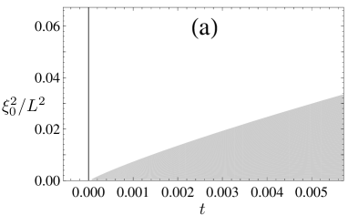
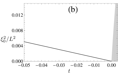
Figure 2: Asymptotic part of the $(\xi_{0}/L)^{1/\nu}$–$t$ plane of the Gaussian model in three dimensions with isotropic short-range interaction in film geometry with NN (a) and DD (b) b.c.. The solid lines indicate the film critical temperatures $T_{\text{c,film}}(L)$ at finite $L$: (a) vertical line at $t=0$ for NN b.c., (b) Eq. (69) for DD b.c.. No low-temperature phases exist for $T<T_{\text{c,film}}(L)$. Finite-size scaling is valid between the film critical lines and the shaded areas. The shaded areas (as defined in the text) are nonscaling regions that depend on $\tilde{a}/\xi_{0}$. Their shapes are shown here for the example $\tilde{a}/\xi_{0}=1$. These shapes start at the origin with infinite slope. The film critical lines in (a) and (b) have the same form as for the cases of periodic and antiperiodic b.c., respectively. In these cases surface terms are absent and only very small nonscaling regions exist due to the nonscaling exponential parts $\sim\exp(-L/\xi_{\text{e}})$ mentioned after Eq. (85).

Because of the dependence of $\ln(\xi/\tilde{a})$ on the nonuniversal lattice spacing $\tilde{a}$, no finite-size scaling functions of $f_{\text{s}}^{\text{(NN)}}(t,L)$ and $f_{\text{s}}^{\text{(DD)}}(t,L)$ can be defined. The nonuniversal surface terms $\sim L^{-1}$ constitute the leading deviations from the bulk critical behavior for large $L$ at fixed $t>0$. One may define “nonscaling regions” in the $(\xi_{0}/L)^{1/\nu}$–$t$ planes (see Figs. 2(a) and (b)) by requiring that these logarithmic terms are comparable to or larger than the scaling terms $L^{-3}\mathcal{G}({\tilde{x}})$. These nonscaling regions depend on $\tilde{a}/\xi_{0}$ and are shown for the example $\tilde{a}/\xi_{0}=1$ as the shaded regions in Figs. 2(a) and (b).

The logarithmic deviations from scaling are not present right at bulk $T_{\text{c}}$, where $f_{\text{s}}(0,L)=L^{-3}\mathcal{G}(0)$ with the universal critical amplitudes $\mathcal{G}^{\text{(NN)}}(0)=\mathcal{G}^{\text{(DD)}}(0)=-\zeta(3)/(16\pi)$, in agreement with Eq. (9.2) for $N=1$ in KrDi92a .

For the remaining part of the discussion we need to distinguish the cases of NN and DD b.c.. For NN b.c., the function $f_{\text{s}}^{\text{(NN)}}(t,L)$ is not regular at $t=0$ as it includes the film critical behavior (76) with (77c) for $t\to 0$ at fixed $L$. To derive this behavior we use the small-${\tilde{x}}$ expansion for ${\tilde{x}}\geq 0$

$$\mathcal{G}^{\text{(NN)}}({\tilde{x}}) =-\frac{\zeta(3)}{16\pi}-\frac{{\tilde{x}}(\ln{\tilde{x}}{+}2\ln 2{-}1)}{16\pi}+\frac{{\tilde{x}}^{3/2}}{12\pi}+O({\tilde{x}}^{2}),$$ (105)

which implies

$$f_{\text{s}}^{\text{(NN)}}(t,L)=f_{\text{s}}^{\text{(NN)}}(0,L)-\frac{1}{L^{3}}\left[\frac{{\tilde{x}}\ln({\tilde{x}}\tilde{a}/L)}{8\pi}+O({\tilde{x}})\right].$$ (106)

The second term yields (77c) because of ${\tilde{x}}=L^{2}/\xi_{\text{film}}^{2}$ for NN b.c..

By contrast, the film critical point for DD b.c. is located at $t_{\text{c,film}}<0$, see (69), thus no singularity exists at $t=0$ for finite $L$ for DD b.c., which implies that $f_{\text{s}}^{\text{(DD)}}(t,L)$ should be regular at $t=0$. This is indeed the case as shown in the following. The first three terms of $f_{\text{s}}^{\text{(DD)}}(t,L)$ from (103) can be rewritten as

$$f_{\text{s}}^{\text{(DD)}}(t,L)$$

$$=\frac{1}{L^{3}}\left[\mathcal{G}^{\text{(DD)}}({\tilde{x}})-\frac{{\tilde{x}}^{3/2}}{12\pi}+\frac{{\tilde{x}}\ln{\tilde{x}}}{16\pi}-\frac{{\tilde{x}}\ln(L/\tilde{a})}{8\pi}\right],$$ (107)

where now the logarithmic deviation from scaling appears in the form of $\ln(L/\tilde{a})$ but the temperature dependence through ${\tilde{x}}\sim t$ is regular at $t=0$ since

$$\mathcal{G}^{\text{(DD)}}({\tilde{x}})-\frac{{\tilde{x}}^{3/2}}{12\pi}+\frac{{\tilde{x}}\ln{\tilde{x}}}{16\pi}$$ (108)

is regular at ${\tilde{x}}=0$ (see Appendix E). It is understood that in (108) for $-\pi^{2}<{\tilde{x}}<0$, the function $\mathcal{G}^{\text{(DD)}}({\tilde{x}})$ means the analytic continuation to ${\tilde{x}}<0$ as given by (IV.3), which is complex; together with the complex terms $-{\tilde{x}}^{3/2}/(12\pi)+{\tilde{x}}\ln{\tilde{x}}/(16\pi)$, however, (108) becomes real and analytic for ${\tilde{x}}>-\pi^{2}$ with a finite real value at ${\tilde{x}}=-\pi^{2}$, see Appendix E. The representation (IV.3) has the advantage that it is valid down to ${\tilde{x}}=-\pi^{2}$ corresponding to the film critical point. For ${\tilde{x}}\to-\pi^{2}$ it includes the film critical behavior (76) with (77d). To derive this behavior we use an expansion around ${\tilde{x}}=-\pi^{2}$ for ${\tilde{x}}>-\pi^{2}$ (see Appendix E),

$$\mathcal{G}^{\text{(DD)}}({\tilde{x}})-\frac{{\tilde{x}}^{3/2}}{12\pi}+\frac{{\tilde{x}}\ln{\tilde{x}}}{16\pi}$$

$$\!=-\frac{\zeta(3)+2\pi^{2}\ln\pi}{16\pi}-\frac{({\tilde{x}}+\pi^{2})[2\ln({\tilde{x}}+\pi^{2})-4\ln\pi-3]}{16\pi}$$

$$\phantom{=}+O(({\tilde{x}}+\pi^{2})^{2}),$$ (109)

which implies

$$f_{\text{s}}^{\text{(DD)}}(t,L)=f_{\text{s}}^{\text{(DD)}}(t_{\text{c,film}},L)$$

$$\phantom{=}+\frac{1}{L^{3}}\left\{-\frac{({\tilde{x}}+\pi^{2})\ln[({\tilde{x}}+\pi^{2})L/\tilde{a})]}{8\pi}+O({\tilde{x}}+\pi^{2})\right\}.$$ (110)

The second term yields (77d) because of ${\tilde{x}}+\pi^{2}=L^{2}/\xi_{\text{film}}^{2}$ for DD b.c..

For ${\tilde{x}}\geq 0$, the $d=3$ scaling functions $\mathcal{G}^{\text{(NN)}}({\tilde{x}})$ and $\mathcal{G}^{\text{(DD)}}({\tilde{x}})$ will be shown in Sec. V together with the corresponding scaling functions $X^{\text{(NN)}}({\tilde{x}})$ and $X^{\text{(DD)}}({\tilde{x}})$ of the Casimir force.

IV.4 ND b.c. in $1<d<4$ dimensions

For ND b.c., the leading terms of the singular parts of the surface free energies, i.e., the $O(\xi^{1-d})$ terms in (90a) and (90b) and the logarithmic terms in (101) and (101), cancel. Then the leading term of the singular part of the total surface free energy density for $t>0$,

$$f_{\text{sf,s}}^{\text{(ND)}}=f_{\text{sf,s}}^{\text{(N)}}(t)+f_{\text{sf,s}}^{\text{(D)}}(t)=-\frac{\Gamma(-\frac{d}{2})}{4(4\pi)^{d/2}}\frac{\tilde{a}}{\xi^{d}}+O(\xi^{-(d+1)}),$$ (111)

does not have the universal scaling form (21), but depends explicitly on $\tilde{a}$. The cancelation of the leading surface terms $\sim\xi^{1-d}$ for ND b.c. was already noted in Appendix C of KrDi92a , where, however, the next-to-leading surface term $\sim\xi^{-d}$, (111), was not taken into account. In contrast to the weak logarithmic deviations from scaling in $d=3$ dimensions according to (101), Eq. (111) constitutes a strong power-law violation of scaling (within the Gaussian model) that has an important impact on the scaling structure of the free energy density in a large part of the $L^{-1/\nu}$–$t$ plane. The resulting singular and nonsingular parts of the free energy density for ND b.c. read for $t\geq 0$

$$f_{\text{s}}^{\text{(ND)}}(t,L)=f_{\text{b,s}}(t)+\frac{1}{L}\left[-\frac{\Gamma(-\frac{d}{2})}{4(4\pi)^{d/2}}\frac{\tilde{a}}{\xi^{d}}\right]+\frac{\mathcal{G}^{\text{(ND)}}({\tilde{x}})}{L^{d}},$$ (112)

$$f_{\text{ns}}^{\text{(ND)}}(t,L)=f_{\text{b,ns}}(t)$$

$$\phantom{=}+\frac{1}{L}\left[f_{\text{sf}}^{\text{(N)}}(0)+f_{\text{sf}}^{\text{(D)}}(0)-\frac{\tilde{b}_{d}^{\text{(N)}}+\tilde{b}_{d}^{\text{(D)}}}{\tilde{a}^{d-1}}\tilde{r}_{0}+O(\tilde{r}_{0}^{2})\right],$$ (113)

where $\tilde{b}_{d}^{\text{(N)}}+\tilde{b}_{d}^{\text{(D)}}<0$ and, for ${\tilde{x}}\geq 0$,

$$\mathcal{G}^{\text{(ND)}}({\tilde{x}})=2^{-d}\mathcal{G}^{\text{(a)}}(4{\tilde{x}}),$$ (114)

with $\mathcal{G}^{\text{(a)}}$ from (83b) (see Appendix B). This result remains valid for $d\to 3$, where $\lim_{d\to 3}(\tilde{b}_{d}^{\text{(N)}}+\tilde{b}_{d}^{\text{(D)}})=\tilde{b}^{\text{(N)}}+\tilde{b}^{\text{(D)}}$ with $\tilde{b}^{\text{(N)}}$ and $\tilde{b}^{\text{(D)}}$ given by (102). For $d\to 2$, the divergent terms of (112) and (IV.4) combine to give a finite result, while $\mathcal{G}^{\text{(ND)}}({\tilde{x}})$ remains finite and continues to provide the scaling function of the finite-size contribution to the free energy.

The representation of our results differs from that of Ref. KrDi92a , where Eqs. (6.8) provide an integral representation of $\mathcal{G}^{\text{(ND)}}$. Both representations have the same expansions in terms of modified Bessel functions, see Appendix C, which suggests that, for ${\tilde{x}}>0$, $\mathcal{G}^{\text{(ND)}}({\tilde{x}})=\Theta_{+\text{O,SB}}^{(1)}(y_{+})$, with the identification $y_{+}=\sqrt{{\tilde{x}}}$. Our representation of $\mathcal{G}^{\text{(ND)}}({\tilde{x}})$ in terms of $\mathcal{G}^{\text{(a)}}({\tilde{x}})$ and thus $\mathcal{I}_{d}^{\text{(p)}}$ has the advantage that it is directly applicable to the bulk critical point at ${\tilde{x}}=0$, whereas the integral representation of $\Theta_{+\text{O,SB}}^{(1)}(y_{+})$ given in Eqs. (6.8) of KrDi92a requires an extra small-$y_{+}$ treatment of the divergent integral so that after multiplication with the prefactor $y_{+}^{d}$ a finite result is obtained. More importantly, the related representation of $\mathcal{F}^{\text{(ND)}}({\tilde{x}})$ in terms of $\mathcal{I}_{d}^{\text{(ND)}}$ provided in Eq. (IV.4) below has the advantage that it is valid also for ${\tilde{x}}\leq 0$ including the film critical point at ${\tilde{x}}=-(\pi/2)^{2}$, whereas the integral representation of $\Theta_{+\text{O,SB}}^{(1)}(y_{+})$ in Eqs. (6.8) of KrDi92a is not suitable for an analytic continuation to the region ${\tilde{x}}<0$.

In (112) the nonscaling structure of the surface term $\sim L^{-1}$ destroys the finite-size scaling form of $f_{\text{s}}^{\text{(ND)}}(t,L)$ above $T_{\text{c}}$ in the regime where the surface term is comparable to or larger than the finite-size term $L^{-d}\mathcal{G}^{\text{(ND)}}({\tilde{x}})$, i.e., in the regime

$$\left(\frac{L}{\xi}\right)^{d-1}\;\frac{\tilde{a}}{\xi}\;\gtrsim\;\left|\frac{4(4\pi)^{d/2}}{\Gamma(-d/2)}\mathcal{G}^{\text{(ND)}}({\tilde{x}})\right|,$$ (115)

with ${\tilde{x}}=(L/\xi)^{1/\nu}$ for ${\tilde{x}}\geq 0$ (this is valid only for $d\neq 2$; for $d=2$ the logarithm in the singular part of the bulk free energy causes deviations from scaling in any case). For $d=3$ this regime is indicated by the shaded area in Fig. 3.

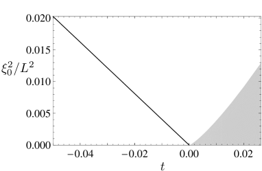
Figure 3: Asymptotic part of the $(\xi_{0}/L)^{1/\nu}$–$t$ plane of the Gaussian model in three dimensions with isotropic short-range interaction in film geometry with ND boundary conditions. The solid line indicates the film critical temperature $T_{\text{c,film}}(L)$ at finite $L$ according to Eq. (70). No low-temperature phase exists for $T<T_{\text{c,film}}$. Finite-size scaling is valid between the film critical line and the shaded area. The shaded area is a nonscaling region that depends on $\tilde{a}/\xi_{0}$. Its shape (shown here for the example $\tilde{a}/\xi_{0}=1$) is determined by Eq. (115). The shape of the shaded area starts at the origin with zero slope.

This violation of finite-size scaling is significantly more important than that due to the exponential correlation length $\xi_{\text{e}}$, (23), which happens only for considerably larger $L\gtrsim 24\xi^{3}/\tilde{a}^{2}$. At fixed $t>0$, the result (112) yields the large–$L$ approach to the bulk critical behavior

$$f_{\text{s}}^{\text{(ND)}}(t,L) -f_{\text{b,s}}(t)=L^{-1}\left[-\frac{\Gamma(-\frac{d}{2})}{4(4\pi)^{d/2}}\frac{\tilde{a}}{\xi^{d}}\right]$$

$$+L^{-d}\frac{{\tilde{x}}^{(d-1)/4}}{2(4\pi)^{(d-1)/2}}e^{-2\sqrt{{\tilde{x}}}}, {\tilde{x}} \gg 1,$$ (116)

see the paragraph around (B). Eq. (IV.4) implies that for $\xi/\tilde{a}\gg 1$ the estimate (115) for the nonscaling region in Fig. 3 can be replaced by $L\gtrsim{\textstyle\frac{1}{2}}\xi\ln(\xi/\tilde{a})$.

The cancelation of the leading surface scaling terms in the Gaussian model does not persist in the $\varphi^{4}$ theory at $O(u^{*})$ (two-loop order) as can be seen from Eq. (D11) of KrDi92a . Two-loop terms, however, are typically smaller than one-loop terms, therefore it is expected that the two-loop contributions to the scaling part are less important than ordinary 1-loop scaling contributions. This means that now corrections to scaling are expected to become considerably more important compared to the scaling part. This would imply a shrinking of the asymptotic region for the case of ND b.c.. Thus we expect that a more careful analysis of future experiments or of MC simulations is required for systems with ND b.c. because of unusually large corrections to scaling.

Above the shaded area in Fig. 3 the nonscaling surface term is negligible and the leading $L$ dependence of $f_{\text{s}}^{\text{(ND)}}(t,L)$ is, for $d\neq 2$, described by the scaling form

$$f_{\text{s}}^{\text{(ND)}}(t,L) =L^{-d}\mathcal{F}^{\text{(ND)}}({\tilde{x}}), {\tilde{x}}\geq-(\pi/2)^{2},$$ (117)

where

$$\mathcal{F}^{\text{(ND)}}({\tilde{x}}) =\mathcal{I}_{d}^{\text{(ND)}}({\tilde{x}}+(\pi/2)^{2})+Y_{d}[{\tilde{x}}+(\pi/2)^{2}]^{d/2}$$

$$=2^{-d}\mathcal{F}^{\text{(a)}}(4{\tilde{x}})$$ (118)

and

$$\mathcal{I}_{d}^{\text{(ND)}}(y)\equiv 2^{-d}\mathcal{I}_{d}^{\text{(a)}}(4y),$$ (119)

with $\mathcal{F}^{\text{(a)}}$ and $\mathcal{I}_{d}^{\text{(a)}}$ from (79b) and (80), respectively. This result includes the film critical behavior (74) and (77e) for ${\tilde{x}}\to-(\pi/2)^{2}$ at fixed finite $L$. To derive this behavior we use an expansion around ${\tilde{x}}=-(\pi/2)^{2}$,

$$\mathcal{I}_{d}^{\text{(ND)}}(y)=\mathcal{I}_{d}^{\text{(ND)}}(0)+Y_{d-1}y^{(d-1)/2}+O(y,y^{d/2}),\\ d\neq 3,$$ (120)

while for $d=3$

$$\mathcal{I}_{3}^{\text{(ND)}}(y) =-\frac{\zeta(3)}{16\pi}-\frac{y[\ln(2y/\pi)-1]}{8\pi}+O(y^{3/2}).$$ (121)

The second terms on the right hand sides of (120) and (121), respectively, yield (74) and (77e) because of ${\tilde{x}}+(\pi/2)^{2}=L^{2}/\xi_{\text{film}}^{2}$.

The universal finite-size amplitude at $T_{\text{c}}$ is

$$\mathcal{F}^{\text{(ND)}}(0) =\mathcal{G}^{\text{(ND)}}(0)=(1-2^{1-d})(4\pi)^{-d/2}\Gamma(d/2)\zeta(d),$$ (122)

which agrees with the corresponding $N=1$ amplitude $\Delta_{\text{O,SB}}^{(1)}$ in Eq. (5.7) of KrDi92a .

For $d=3$ we combine (86b) and (IV.4) to obtain

$$\mathcal{F}^{\text{(ND)}}({\tilde{x}}) =\mathcal{G}^{\text{(ND)}}({\tilde{x}})-\frac{1}{12\pi}{\tilde{x}}^{3/2},$$ (123)

$$\mathcal{G}^{\text{(ND)}}({\tilde{x}}) =-\frac{1}{16\pi}\left[\operatorname{Li}_{3}(-e^{-2\sqrt{{\tilde{x}}}})+2\sqrt{{\tilde{x}}}\operatorname{Li}_{2}(-e^{-2\sqrt{{\tilde{x}}}})\right].$$ (124)

With the identification $y_{+}=\sqrt{{\tilde{x}}}$ we find that $\mathcal{G}^{\text{(ND)}}({\tilde{x}})$ agrees with the more elaborate representation of $\Theta_{+\text{O,SB}}(y_{+})$ provided by Eq. (9.3) in Ref. KrDi92a . Because of the relations (114) and (IV.4), the situation is similar to that explained after (86) and (87), thus $\mathcal{F}^{\text{(ND)}}({\tilde{x}})$ is real for ${\tilde{x}}\geq-(\pi/2)^{2}$ and an analytic function for ${\tilde{x}}>-(\pi/2)^{2}$, even though the analytic continuation of $\mathcal{G}^{\text{(ND)}}({\tilde{x}})$ to negative ${\tilde{x}}$ becomes complex. For ${\tilde{x}}\geq 0$, the $d=3$ scaling function $\mathcal{G}^{\text{(ND)}}({\tilde{x}})$ will be shown in Sec. V together with the corresponding scaling function $X^{\text{(ND)}}({\tilde{x}})$ of the Casimir force.

In the region where finite-size scaling is valid (see Fig. 3) there exists a scaling function $\mathcal{F}^{\text{(ND)}}({\tilde{x}})$ of the free energy density for ${\tilde{x}}\geq-(\pi/2)^{2}$. Due to Eqs. (114) and (IV.4), a plot of this function in three dimensions can be obtained from the solid curve in Fig. 1 with appropriately rescaled axes (the same holds for $\mathcal{G}^{\text{(ND)}}({\tilde{x}})$ and the bulk part $Y_{3}{\tilde{x}}^{3/2}$).

V Casimir force

The excess free energy density per component divided by $k_{\text{B}}T$ is defined by

$$f_{\text{ex}}(t,L)=f(t,L)-f_{\text{b}}(t),$$ (125)

where $f_{\text{b}}(t)$, (II.1), is the bulk free energy density. The latter exists only for $t\geq 0$. Thus, as a shortcoming of the Gaussian model, $f_{\text{ex}}(t,L)$ can be defined only for $t\geq 0$ although $f(t,L)$, (II.1), exists for $t<0$ for the cases of antiperiodic, DD, and ND boundary conditions.

The Casimir force $F_{\text{Cas}}$ per component and per unit area divided by $k_{\text{B}}T$ is related to $f_{\text{ex}}$ by

$$F_{\text{Cas}}(t,L)/(k_{\text{B}}T)=-\frac{\partial[Lf_{\text{ex}}(t,L)]}{\partial L}.$$ (126)

For the subclass of isotropic systems, the asymptotic scaling form of its singular contribution is

$$F_{\text{Cas,s}}(t,L)/(k_{\text{B}}T)=L^{-d}X({\tilde{x}}),$$ (127)

where, for ${\tilde{x}}\geq 0$, the universal scaling function $X({\tilde{x}})$ is determined by the universal scaling function $\mathcal{G}({\tilde{x}})$ of the finite-size contribution to the free energy defined by (II.1) according to

$$X({\tilde{x}}) =(d-1)\mathcal{G}({\tilde{x}})-\nu^{-1}{\tilde{x}}\frac{d\mathcal{G}({\tilde{x}})}{d{\tilde{x}}}.$$ (128)

The surface contributions to the free energy density do not contribute to $X({\tilde{x}})$. As an important consequence, finite-size scaling is found to be valid for the Casimir force for all b.c. in $1<d<4$ dimensions, i.e., no scaling violations exist for the Casimir force in the three-dimensional Gaussian model with NN, DD, and ND b.c., in contrast to the free energy density itself.

As a consequence of (II.3), the asymptotic scaling form of the singular part of the Casimir force becomes nonuniversal in the case of the anisotropic couplings (51). Then (127) is replaced by

$$F_{\text{Cas,s}} (t,L)/(k_{\text{B}}T)$$

$$=L^{-d}(J_{\perp}/J_{\parallel})^{(d-1)/2}X(t(L/\xi_{0,\perp})^{1/\nu}),$$ (129)

where $\xi_{0,\perp}$ is the amplitude of the correlation length (56b). Thus the Casimir force depends explicitly on the ratio of the microscopic couplings $J_{\perp}$ and $J_{\parallel}$ for all b.c., in agreement with earlier results for periodic ChDo04 ; Do08a and antiperiodic dan09 b.c.. In the following we primarily discuss the isotropic case.

For ${\tilde{x}}\geq 0$ follow from (128) with (IV.2) and (114)

$$X^{\text{(NN)}}({\tilde{x}})=X^{\text{(DD)}}({\tilde{x}}) =2^{-d}X^{\text{(p)}}(4{\tilde{x}}),$$ (130a)

$$X^{\text{(ND)}}({\tilde{x}}) =2^{-d}X^{\text{(a)}}(4{\tilde{x}}),$$ (130b)

and with (83b)

$$X^{\text{(a)}}({\tilde{x}})=2^{1-d}X^{\text{(p)}}(4{\tilde{x}})-X^{\text{(p)}}({\tilde{x}}).$$ (131)

Thus we only need $X^{\text{(p)}}$, which we obtain in $1<d<4$ dimensions by applying (128) to (83a). In three dimensions we utilize (87a), its derivative

$$\frac{d\mathcal{G}^{\text{(p)}}({\tilde{x}})}{d{\tilde{x}}}=-\frac{1}{4\pi}\ln\left(1-e^{-\sqrt{{\tilde{x}}}}\right),$$ (132)

and (131) to obtain the $d=3$ scaling functions for periodic and antiperiodic b.c. for ${\tilde{x}}\geq 0$,

$$X^{\text{(p)}}({\tilde{x}}) =-\frac{1}{\pi}\left[\operatorname{Li}_{3}(e^{-\sqrt{{\tilde{x}}}})+\sqrt{{\tilde{x}}}\operatorname{Li}_{2}(e^{-\sqrt{{\tilde{x}}}})\right]$$

$$\phantom{=}+\frac{{\tilde{x}}}{2\pi}\ln\left(1-e^{-\sqrt{{\tilde{x}}}}\right)$$

$$=-\frac{\zeta(3)}{\pi}+\frac{{\tilde{x}}}{4\pi}-\frac{{\tilde{x}}^{3/2}}{12\pi}+O({\tilde{x}}^{2}),$$ (133a)

$$X^{\text{(a)}}({\tilde{x}}) =-\frac{1}{\pi}\left[\operatorname{Li}_{3}(-e^{-\sqrt{{\tilde{x}}}})+\sqrt{{\tilde{x}}}\operatorname{Li}_{2}(-e^{-\sqrt{{\tilde{x}}}})\right]$$

$$\phantom{=}+\frac{{\tilde{x}}}{2\pi}\ln\left(1+e^{-\sqrt{{\tilde{x}}}}\right)$$

$$=\frac{3\zeta(3)}{4\pi}-\frac{{\tilde{x}}^{3/2}}{12\pi}+O({\tilde{x}}^{2}).$$ (133b)

The scaling functions for the other b.c. follow by employing (130).

At ${\tilde{x}}=0$ the critical Casimir amplitude Kr94

$$\Delta\equiv(d-1)^{-1}X(0)$$ (134)

is obtained for $1<d<4$ as

$$\Delta^{\text{(p)}}\! =2^{d}\Delta^{\text{(NN)}}\!=2^{d}\Delta^{\text{(DD)}}=-\pi^{-d/2}\Gamma({\textstyle\frac{d}{2}})\zeta(d),$$ (135a)

$$\Delta^{\text{(a)}}\! =2^{d}\Delta^{\text{(ND)}}\!=(2^{1-d}-1)\Delta^{\text{(p)}},$$ (135b)

specializing for $d=3$ to

$$\Delta^{\text{(p)}}\!\! =8\Delta^{\text{(NN)}}\!=8\Delta^{\text{(DD)}}=-\frac{\zeta(3)}{2\pi}\approx-0.191313,$$ (136a)

$$\Delta^{\text{(a)}}\!\! =8\Delta^{\text{(ND)}}\!=\frac{3\zeta(3)}{8\pi}\approx 0.143485.$$ (136b)

The results (135) are identical to the results (5.6) and (5.7) of KrDi92a after setting $N=1$ (there is a misprint concerning the sign of $\Delta_{\text{per}}^{(1)}$ in (5.7) of KrDi92a ). The results for $\Delta^{\text{(p)}}$ are also in agreement with Eq. (3.42) of DaKr04 .

As a consequence of (V), the Casimir amplitude $\Delta_{\text{aniso}}$ of the anisotropic system (with $J_{\perp}\neq J_{\parallel}$) is nonuniversal and is related to $\Delta$ of the isotropic system (with $J=J_{\perp}=J_{\parallel}$) for all b.c. by

$$\Delta_{\text{aniso}}=(J_{\perp}/J_{\parallel})^{(d-1)/2}\Delta=(\xi_{0,\perp}/\xi_{0,\parallel})^{d-1}\Delta,$$ (137)

in agreement with earlier results for periodic ChDo04 and antiperiodic dan09 b.c.. For $d=2$, the right hand side of (5.13) is of the same form as found in Indekeu for the anisotropic Ising model on a two-dimensional strip with free b.c..

VI Casimir force in $d=2$ dimensions

Our exact results for $X_{\text{Gauss}}$ in $d=2$ dimensions are of particular interest in view of results for the exact Casimir force scaling functions $X_{\text{Ising}}$ for an Ising model with isotropic couplings on a two-dimensional strip of infinite length and finite width $L$ for free b.c. Evans and for periodic and antiperiodic b.c. in the recent work by Rudnick et al. RuZaShAb10 . Moreover, there exist earlier results for the Casimir amplitude at $T_{\text{c}}$ of the two-dimensional Ising model with free b.c. and anisotropic couplings by Indekeu et al. Indekeu . This calls for a comparison with the corresponding Gaussian model results $X_{\text{Gauss}}$.

VI.1 Isotropic case

For the isotropic case, the two-dimensional Gaussian model results for periodic, antiperiodic, and DD b.c. are obtained from Eqs. (80), (83a), (128), (130a), and (131) for $d=2$. They read

$$X_{\text{Gauss}}^{\text{(p)}}({\tilde{x}}) =-\frac{1}{2\pi}\int_{0}^{\infty}dz\left(\frac{\pi}{z}\right)^{3/2}\left(1+\frac{z{\tilde{x}}}{2\pi^{2}}\right)\times$$

$$~{}~{}~{}~{}~{}~{}e^{-z{\tilde{x}}/(2\pi)^{2}}\left[K(z)-\sqrt{\frac{\pi}{z}}\right],$$ (138a)

$$X_{\text{Gauss}}^{\text{(a)}}({\tilde{x}}) ={\textstyle\frac{1}{2}}X_{\text{Gauss}}^{\text{(p)}}(4{\tilde{x}})-X_{\text{Gauss}}^{\text{(p)}}({\tilde{x}}),$$ (138b)

$$X_{\text{Gauss}}^{\text{(DD)}}({\tilde{x}}) ={\textstyle\frac{1}{4}}X_{\text{Gauss}}^{\text{(p)}}(4{\tilde{x}}),$$ (138c)

with the scaling variable ${\tilde{x}}=(L/\xi_{0})^{1/\nu}t=(L/\xi)^{2}$, $\nu=1/2$, $t\,{\geq}\,0$. Above $T_{\text{c}}$, the corresponding Ising model results for periodic, antiperiodic, and free b.c. read Evans ; RuZaShAb10

$$X_{\text{Ising}}^{\text{(p)}}(x_{\text{I}}) =\frac{1}{2\pi}\int_{0}^{\infty}\!d\omega\,q\left[\tanh(q/2)-1\right],$$ (139a)

$$X_{\text{Ising}}^{\text{(a)}}(x_{\text{I}}) =\frac{1}{2\pi}\int_{0}^{\infty}\!d\omega\,q\left[\coth(q/2)-1\right],$$ (139b)

$$X_{\text{Ising}}^{\text{(free)}}(x_{\text{I}}) =\frac{1}{2\pi}\int_{0}^{\infty}\!d\omega\,q\left[\frac{\left(q{+}x_{\text{I}}\right)e^{q}-\left(q{-}x_{\text{I}}\right)e^{-q}}{\left(q{+}x_{\text{I}}\right)e^{q}+\left(q{-}x_{\text{I}}\right)e^{-q}}{-}1\right],$$ (139c)

with $q\equiv\sqrt{x_{\text{I}}^{2}+\omega^{2}}$. Here our Ising scaling variable $x_{\text{I}}=(L/\xi_{0,I})^{1/\nu}t=L/\xi$ with $\nu=1$ and $\xi_{0,I}=(8\beta_{c}J)^{-1}$ exp.corr.length is related to the scaling variables $X$ and $x$ used in Evans and RuZaShAb10 , respectively, by $x_{\text{I}}=2X=2x$ (compare, e.g., with the isotropic limit of the correlation-length results in Appendix A 2 of Indekeu ; see also Sec. VI.2 below). As an unexpected result, we find the surprising identities

$$X^{\text{(p)}}_{\text{Gauss}}((L/\xi)^{2}) =-X^{\text{(a)}}_{\text{Ising}}(L/\xi),$$ (140a)

$$X^{\text{(a)}}_{\text{Gauss}}((L/\xi)^{2}) =-X^{\text{(p)}}_{\text{Ising}}(L/\xi),$$ (140b)

whose derivation will be presented elsewhere KaDo10 .

For a comparison of these results see Fig. 4. In Fig. 4(b), we have assumed that (asymptotically close to criticality) free b.c. in the Ising model correspond to DD b.c. in the Gaussian model. We see some similarity on a qualitative level: both the Gaussian and the Ising scaling functions are negative for periodic and for DD (or free) b.c., thus implying an attractive Casimir force whereas for antiperiodic b.c. they are positive implying a repulsive Casimir force. On a quantitative level, however, the Casimir amplitudes at $T_{\text{c}}$ differ significantly, namely by a factor of two according to the exact results $X^{\text{(p)}}_{\text{Gauss}}(0)=2X^{\text{(p)}}_{\text{Ising}}(0)=-\pi/6$, $2X^{\text{(a)}}_{\text{Gauss}}(0)=X^{\text{(a)}}_{\text{Ising}}(0)=\pi/6$, and $X^{\text{(DD)}}_{\text{Gauss}}(0)=2X^{\text{(free)}}_{\text{Ising}}(0)=-\pi/24$, obtained from (134), (135), and (139). Furthermore we note that, according to the dashed line in Fig. 4(a), $X^{\text{(a)}}_{\text{Gauss}}$ has a weak maximum above $T_{\text{c}}$, and correspondingly $X^{\text{(p)}}_{\text{Ising}}$ has a weak minimum above $T_{\text{c}}$, in agreement with Fig. 2 of RuZaShAb10 and Fig. 15 of VaGaMaDi08 .

These results can be interpreted in terms of the two-dimensional $\varphi^{4}$ model which should be in the same universality class as the two-dimensional Ising model. In all cases, the scaling functions at $T_{\text{c}}$ of the Gaussian model differ by a factor of two from the scaling functions at $T_{\text{c}}$ of the two-dimensional $\varphi^{4}$ model. This indicates that a low-order perturbation approach in the two-dimensional $\varphi^{4}$ model (in terms of a perturbation expansion with respect to the four-point coupling) is inappropriate, in contrast to the situation in three dimensions to be discussed in Sec. VII. This is quite plausible since the fixed-point value of the renormalized four-point coupling in two dimensions is quite large, i.e., far from the vanishing Gaussian fixed-point value. This is in line with the known fact that non-Gaussian fluctuations are generally larger in two than in three dimensions, as seen, e.g., from the bulk critical exponents.

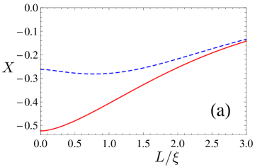
Figure 4: (Color online) Casimir force scaling functions (138) and (139) of the Gaussian and Ising models in $d=2$ dimensions. (a) Scaling functions $X^{\text{(p)}}_{\text{Gauss}}((L/\xi)^{2})=-X^{\text{(a)}}_{\text{Ising}}(L/\xi)$ (solid line) according to (140a) and $X^{\text{(p)}}_{\text{Ising}}((L/\xi)^{2})=-X^{\text{(a)}}_{\text{Gauss}}(L/\xi)$ (dashed line) according to (140b). (b) Scaling functions $X^{\text{(DD)}}_{\text{Gauss}}((L/\xi)^{2})$ (solid line) and $X^{\text{(free)}}_{\text{Ising}}(L/\xi)$ (dashed line).

VI.2 Anisotropic case

We have extended the analysis of the isotropic Ising model by Rudnick et al. RuZaShAb10 for periodic and antiperiodic b.c. to the anisotropic Ising model on a square lattice with nearest-neighbor couplings $J_{\parallel}>0$ and $J_{\perp}>0$. This corresponds to the “rectangular lattice” of Indekeu et al. Indekeu with the identifications of the couplings $K_{1}=2\beta J_{\parallel}$, $K_{2}=2\beta J_{\perp}$, and $K_{3}=0$. The corresponding bulk-correlation-length amplitudes above $T_{\text{c}}$ follow from Appendix A 2 of Indekeu (for $\tilde{a}=1$) as exp.corr.length

$$\xi_{0,\perp} =\frac{1}{4}\left(\beta_{c}J_{\parallel}+\frac{\beta_{c}J_{\perp}}{\sinh(4\beta_{c}J_{\perp})}\right)^{-1},$$ (141a)

$$\xi_{0,\parallel} =\frac{1}{4}\left(\beta_{c}J_{\perp}+\frac{\beta_{c}J_{\parallel}}{\sinh(4\beta_{c}J_{\parallel})}\right)^{-1},$$ (141b)

with the ratio (66), where we have used the condition $\sinh(4\beta_{c}J_{\parallel})\sinh(4\beta_{c}J_{\perp})=1$ for $d=2$ bulk criticality. From Sec. II.3 we obtain the nonuniversal Casimir force scaling function of the anisotropic Gaussian model for $d>2$ above $T_{\text{c}}$

$$X_{\text{aniso}} (t(L/\xi_{0,\perp})^{1/\nu};J_{\parallel},J_{\perp})$$

$$=(\xi_{0,\perp}/\xi_{0,\parallel})^{d-1}X_{\text{iso}}(t(L/\xi_{0,\perp})^{1/\nu}).$$ (142)

We have verified that this relation holds also for $d=2$ dimensions (i) for the Gaussian model with periodic, antiperiodic, DD, NN, and ND b.c. and (ii) for the Isingmodel for periodic and antiperiodic b.c.. There is little doubt that it also holds for the two-dimensional Ising model with corresponding other b.c.. Right at $T_{\text{c}}$ this was established already in Indekeu for the case of free b.c., as noted in Sec. II.C .

VII $\varphi^{4}$ field theory at $d=3$

In this section we present the first (one-loop) step within the framework of the minimally renormalized $\varphi^{4}$ field theory at fixed dimensions $2<d<4$ dohm ; Do08a for the calculation of the Casimir force scaling function in film geometry in the regime $T\geq T_{\text{c}}$ for all five b.c. defined in Sec. II. As noted in Sec. II.3, our Gaussian results for the various scaling functions $\mathcal{G}({\tilde{x}})$ and $X({\tilde{x}})$ can be incorporated in such a theory based on the isotropic $\varphi^{4}$ Hamiltonian (41). We emphasize, however, that we do not set $u_{0}$ equal to zero from the outset and that our one-loop treatment goes beyond the simple Gaussian model in that it includes the effect of the renormalized four-point coupling $u$ via the exact exponent function $\zeta_{r}(u)$ (see Eq. (146) below), whose fixed-point value determines the exact (non-Gaussian) critical exponent $\nu$. The one-loop approximation manifests itself only in neglecting the (two-loop) $O(u^{*})$ contribution to the amplitude function of the free energy density. Such a treatment has recently been presented in Sec. X A of Do08a for the case of cubic geometry with periodic b.c.. For the specific heat in film geometry with Dirichlet b.c. a corresponding treatment was given in sutter . As suggested by the earlier successes sutter ; Do08a ; Do08b , the minimally renormalized $\varphi^{4}$ theory at fixed $d$ is expected to constitute an important alternative in the determination of the Casimir force scaling function in comparison to the earlier $\varepsilon$ expansion approach KrDi92a ; KrDi92b ; GrDi07 . Our quantitative results to be presented in Fig. 5 below will support this expectation. Other fixed-$d$ renormalization schemes are, of course, conceivable which would lead to the same one-loop results at $d=3$ as obtained in our approach. We believe, however, that the fixed-$d$ minimal subtraction scheme has considerable advantages in extending the finite-size theory to two-loop order and to the temperature regime below $T_{\text{c}}$ Do08a ; Do08b .

As a temperature variable we use the shifted parameter $r_{0}-r_{\text{0c}}=a_{0}t$, where $r_{\text{0c}}=-4(n+2)u_{0}\int_{\bm{k}}^{(d)}\bm{k}^{-2}$ is the critical value of $r_{0}$ up to $O(u_{0})$. In the following we sketch the relevant steps of calculating the singular part of the minimally renormalized free energy density in one-loop order for film geometry with periodic or antiperiodic b.c.. After subtracting the regular bulk part up to linear order in $r_{0}-r_{0c}$ and performing the limit $\Lambda\to\infty$ at fixed $r_{0}-r_{0c}$ we obtain the bare one-loop expression of the remaining part $\delta f$ of the free energy density per component divided by $k_{B}T$ in $2<d<4$ dimensions as

$$\delta f(r_{0}-r_{0c}, u_{0},L)=-\frac{A_{d}}{d\varepsilon}\;(r_{0}-r_{0c})^{d/2}$$

$$+L^{-d}\mathcal{G}((r_{0}-r_{0c})L^{2})+O(u_{0})$$ (143)

for periodic and antiperiodic b.c. where $\mathcal{G}^{\text{(p)}}(y)$ and $\mathcal{G}^{\text{(a)}}(y)$ are given by (83a) and (83b). The renormalized parameters $r$ and $u$ are defined in the standard way Do08a as $r=Z_{r}^{-1}(r_{0}-r_{0c})$ and $u=\mu^{-\varepsilon}A_{d}Z_{u}^{-1}Z_{\varphi}^{2}u_{0}$ with an inverse reference length $\mu=\xi_{0}^{-1}$, where $\xi_{0}$ is the correlation-length amplitude above $T_{\text{c}}$. The additively renormalized counterpart $f_{R}$ of $\delta f$ is defined as Do08a

$$f_{R}(r,u,L,\mu) =\delta f(Z_{r}r,\mu^{\varepsilon}Z_{u}Z_{\varphi}^{-2}A_{d}^{-1}u,L)$$

$$\phantom{=}-\frac{1}{8}\mu^{-\varepsilon}n^{-1}r^{2}A_{d}A(u,\varepsilon),$$ (144)

where $A(u,\varepsilon)=-2n/\varepsilon+O(u)$ is the additive renormalization constant of the minimal renormalization scheme. After integration of the renomalization-group equation (see Eqs. (5.6) and (5.7) of Do08a ) and with the choice $\mu^{2}l^{2}=r(l)$ of the flow parameter $l$, the finite-size part of $f_{R}$ is then given by

$$f_{R}(r,u,L,\mu)-f_{R}(r,u,\infty,\mu) =L^{-d}\mathcal{G}(r(l)L^{2})+O(u(l)),$$ (145)

with the effective temperature variable dohm

$$r(l) =r\exp\left(\int_{1}^{l}\zeta_{r}(u(l^{\prime}))\frac{dl^{\prime}}{l^{\prime}}\right).$$ (146)

This variable contains the field-theoretic function $\zeta_{r}(u)=\mu(\partial_{\mu}\ln Z_{r}^{-1})_{0}$ dohm with the fixed point value $\zeta_{r}(u^{*})=2-\nu^{-1}$. Asymptotically ($l\to 0$), this leads to the scaling form of the singular part of the excess free energy per component in one-loop order

$$f_{\text{ex,s}}(t,L) =L^{-d}\mathcal{G}(L^{2}/\xi^{2})+O(u^{*})$$ (147)

for periodic and antiperiodic b.c., with $\mathcal{G}^{\text{(p)}}(y)$ and $\mathcal{G}^{\text{(a)}}(y)$ given by (83a) and (83b) where now $\xi=\xi_{0}t^{-\nu}$ is the correlation length above $T_{\text{c}}$ with the exact critical exponent $\nu$ of the $(d,n)$ universality class.

A complication appears to arise at $d=3$ for NN and DD b.c. because in these cases the limit $\Lambda\to\infty$ at fixed $r_{0}-r_{0c}$ does not exist which in the dimensionally regularized form of the free energy density shows up as pole terms at $d=3$. These divergent contributions, however, are restricted only to the surface part $L^{-1}f_{\text{sf}}$ which does not contribute to the Casimir force. Thus $f_{\text{ex}}(t,L)-L^{-1}f_{\text{sf}}(t)$ is well behaved at $d=3$ in the limit $\Lambda\to\infty$ at fixed $r_{0}-r_{0c}$. Consequently there exists no problem in the calculation of the finite-size part scaling function $\mathcal{G}$ and of the Casimir force scaling function $X$ in the framework of the minimally renormalized theory at fixed $d=3$ for NN and DD b.c.. This holds also for ND b.c.. The resulting asymptotic scaling form in one-loop order is

$$f_{\text{ex,s}}(t,L)-L^{-1}f_{\text{sf,s}}(t) =L^{-d}\mathcal{G}(L^{2}/\xi^{2})+O(u^{*}),$$ (148)

for NN, DD, and ND b.c., where $\mathcal{G}^{\text{(NN)}}(y)$, $\mathcal{G}^{\text{(DD)}}(y)$, and $\mathcal{G}^{\text{(ND)}}(y)$ are given by (IV.2) with (83a), and by (114) with (83b), respectively. Again, the correlation length $\xi$ in (148) contains the exact critical exponent $\nu$ of the $(d,n)$ universality class. The results (147) and (148) can be applied directly to $d=3$ dimensions. The Casimir force scaling functions $X(L^{2}/\xi^{2})$ follow from (128). Thus we are in the position to perform a reasonable comparison both with MC data for the three-dimensional Ising model VaGaMaDi08 and with earlier $\varepsilon=4-d$ expansion results KrDi92a ; GrDi07 of the $\varphi^{4}$ theory evaluated at $\varepsilon=1$ as well as with the very recent result of an improved $d=3$ perturbation theory Do08b (in a ${L_{\parallel}^{2}\times L}$ slab geometry with a finite aspect ratio $\rho=L/L_{\parallel}=1/4$) for periodic b.c.. This comparison is one of the central results of this paper.

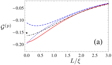
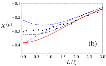
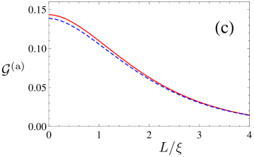
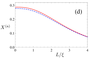
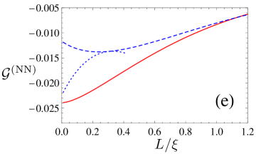
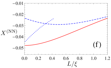
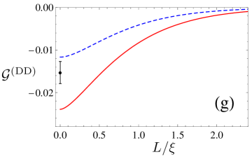
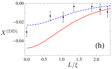
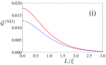
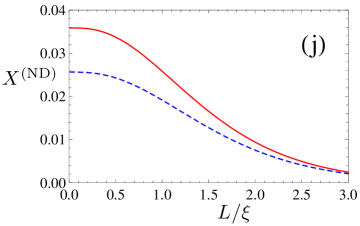
Figure 5: (Color online) Scaling functions $\mathcal{G}$ and $X$ of the finite-size part of the free energy density and of the Casimir force, respectively, for $T\geq T_{\text{c}}$ in a three-dimensional film of thickness $L$ with isotropic interactions for the various b.c. as a function of the scaling argument $L/\xi$. Solid lines: one-loop results of the fixed $d=3$ $\varphi^{4}$ theory according to Eqs. (87), (IV.3), (124), (147), and (148) for $\mathcal{G}((L/\xi)^{2})$ and according to Eqs. (130), (133), and (128) for $X((L/\xi)^{2})$. Dashed lines in left panels: two-loop $\varepsilon$ expansion results $\Theta_{+\text{per}}(L/\xi)$, $\Theta_{+\text{aper}}(L/\xi)$, $\Theta_{+\text{SB,SB}}(L/\xi)$, $\Theta_{+\text{O,O}}(L/\xi)$, and $\Theta_{+\text{O,SB}}(L/\xi)$ at $\varepsilon=1$ for $n=1$ for periodic, antiperiodic, NN, DD, and ND b.c., respectively, according to Eqs. (6.12) and (6.13) in KrDi92a . Dashed lines in right panels: two-loop $\varepsilon$ expansion results $\vartheta_{+\text{per}}(L/\xi)$, $\vartheta_{+\text{aper}}(L/\xi)$, $\vartheta_{+\text{SB,SB}}(L/\xi)$, $\vartheta_{+\text{O,O}}(L/\xi)$, and $\vartheta_{+\text{O,SB}}(L/\xi)$ at $\varepsilon=1$ for $n=1$, obtained through Eq. (3.9) in KrDi92b . Dotted line in (a): improved $\varepsilon$ expansion result $\Theta^{(\text{per})}(L/\xi)$ at $\varepsilon=1$ for $n=1$ according to Eq. (4.57) in GrDi07 , compare Fig. 6 of GrDi07 . Dot-dashed line in (a): $F^{\text{ex}}((L/\xi)^{1/\nu},\rho=1/4)$ in fixed $d=3$ according to Eq. (17) in Do08b . Data point in (a): From MC result $\vartheta_{\text{P}}(0)=-0.3040(4)$ in VaGaMaDi08 . Dotted line in (b): improved $\varepsilon$ expansion results $\Xi^{(\text{per})}(L/\xi)$ for $n=1$, obtained through Eq. (1.7) in GrDi07 . Dot-dashed line in (b): $X((L/\xi)^{1/\nu},\rho=1/4)$ in fixed $d=3$ according to Eq. (19) in Do08b . The $L/\xi=0$ data point in (b) is twice the $L/\xi=0$ data point displayed in (a). Other data points in (b): MC results from Fig. 15 in VaGaMaDi08 for $L=20$ and $\rho=1/6$. Dotted line in (e): improved $\varepsilon$ expansion result $\Theta^{(\text{sp,sp})}(L/\xi)$ at $\varepsilon=1$ for $n=1$ according to Eqs. (4.47), (4.50), (4.53), and (4.56) in GrDi07 , compare Fig. 8 of GrDi07 (where the variable on the abscissa should read $\sqrt{L/\xi_{\infty}}=\sqrt{\sf L}$). Dotted line in (f): improved $\varepsilon$ expansion results $\Xi^{(\text{sp,sp})}(L/\xi)$ at $\varepsilon=1$ for $n=1$, obtained through Eq. (1.7) in GrDi07 . Data point in (g): MC result for $L=20$ and $\rho=1/6$ by dividing the $L/\xi=0$–result displayed in (h) by $2$. Data points in (h): MC results for $L=20$ and $\rho=1/6$ from the inset of Fig. 13 in VaGaMaDi08 (where the $\varepsilon$ expansion line is misrepresented).

The comparison is shown in Figs. 5(a)–(j) as a function of the variable $L/\xi$. The solid lines represent our one-loop results. The $\varepsilon$ expansion results are represented by the dashed lines (two-loop $\varepsilon$ expansion KrDi92a ) and by the dotted lines (improved $\varepsilon$ expansion GrDi07 ), respectively, and the result of the improved $d=3$ perturbation theory Do08b is represented by dot-dashed lines in Figs. 5(a),(b). In the large–$L/\xi$ regime (not shown in Fig. 5), the solid and dashed lines have an exponential approach to zero and differ very little from each other in all cases. This statement holds also for the dotted and dot-dashed lines for the case of periodic b.c. (Figs. 5 (a),(b)) but not for the dotted lines for the case of NN b.c. (Figs. 5 (e),(f)), where the $\varepsilon$ expansion result of GrDi07 breaks down in the large–$L/\xi$ regime. Also shown are recent MC data VaGaMaDi08 for the three-dimensional Ising model (in a ${L_{\parallel}^{2}\times L}$ slab geometry with the aspect ratio $\rho=L/L_{\parallel}=1/6$ and with $L=20$) for the cases of periodic and DD b.c. in Figs. 5 (a),(b),(g),(h), respectively.

For periodic b.c., our one-loop result for $\mathcal{G}^{\text{(p)}}(L^{2}/\xi^{2})$ and $X^{\text{(p)}}(L^{2}/\xi^{2})$ (solid lines in Figs. 5(a) and (b)) is in remarkable agreement with the improved $\varepsilon$ expansion result of GrDi07 (dotted lines in Figs. 5(a) and (b)) at $T_{\text{c}}$ (i.e., $L/\xi=0$) and in the large–$L/\xi$ regime. The slope of our one-loop result at $T_{\text{c}}$ is in better agreement with the slope of the MC data than the slopes of the $\varepsilon$ expansion results at $T_{\text{c}}$. In particular, there is no artifact of the one-loop result of the fixed $d=3$ theory such as the minimum of the two-loop $\varepsilon$ expansion result above $T_{\text{c}}$ shown by the dashed line in Figs. 5(a) and (b). This suggests that, for periodic b.c., the $d=3$ approach is a better starting point of perturbation theory than the $\varepsilon$ expansion around $d=4$ dimensions. This is consistent with recent findings of finite-size effects in cubic geometry (Fig. 5 in Do08a ) and in finite-slab geometry (Fig. 4 in Do08b ). For antiperiodic b.c. (see Figs. 5(c) and (d)), there is surprisingly good agreement between our one-loop $d=3$ result for $\mathcal{G}^{\text{(a)}}(L^{2}/\xi^{2})$ and $X^{\text{(a)}}(L^{2}/\xi^{2})$ and the two-loop $\varepsilon$ expansion result KrDi92a . This is quite remarkable in view of the fact that the computational effort in obtaining $d=3$ one-loop RG results is considerably smaller than that for deriving two-loop $\varepsilon$ expansion results.

For NN, DD, and ND b.c., there are considerable differences between our one-loop results of the fixed $d=3$ $\varphi^{4}$ theory and the two-loop $\varepsilon$ expansion results as shown in Figs. 5(e)–(j). For NN b.c., however, the improved $\varepsilon$ expansion result of GrDi07 at $T_{\text{c}}$ is not far from our one-loop result, but for $L/\xi>0$ our $d=3$ result does not agree with the strong increase of the $\varepsilon$ expansion result of GrDi07 .

In summary, the fixed $d=3$ theory yields reasonable results already in one-loop order. It would be a rewarding task to perform a two-loop calculation of the fixed $d$ theory for all b.c. as well as to proceed to higher-orders of the $\varepsilon$ expansion for DD and ND b.c.. Also MC data for the cases of antiperiodic, NN, and ND b.c. are highly desirable for a comparison with the predictions shown in Fig. 5 in order to clarify the reliability of the different perturbative approaches.

VIII Dimensional crossover: Specific heat

In the following, we present an explicit study of the dimensional crossover in the Gaussian model from the finite-size critical behavior near the $d$-dimensional bulk transition at $T_{\text{c}}$ to the $(d{-}1)$-dimensional critical behavior near the film transition at the critical temperature $T_{\text{c,film}}(L)\leq T_{\text{c}}$ of the film of finite thickness $L$. (The equality sign holds only for periodic and NN b.c., whereas $T_{\text{c,film}}(L)<T_{\text{c}}$ for antiperiodic, DD, and ND b.c..) The most interesting candidate for this study is the divergent specific heat $C(t,L)$, whose $d$-dependent critical exponent $\alpha$ changes from $\alpha_{\text{bulk}}=(4-d)/2$ near bulk $T_{\text{c}}$ (see Eq. (28)) to $\alpha_{\text{film}}=[4-(d-1)]/2$ near $T_{\text{c,film}}(L)$ in $d<4$ dimensions. We shall verify that the film critical behavior of a $d$-dimensional system corresponds to that of a bulk system in $d-1$ dimensions for all b.c. except for antiperiodic b.c., where an unexpected factor of two appears due to a two-fold degeneracy of the lowest mode as noted already in Sec. II.1 above. It remains to be seen which effect this feature may have in non-Gaussian models and in the $\varphi^{4}$ theory.

The dimensional crossover behavior is particularly simple in the Gaussian model because the correlation-length exponent $\nu=1/2$ is independent of the dimension $d$ and the correlation-length amplitude is the same both for the bulk and the film critical point. To the best of our knowledge, this crossover behavior has not been presented in the literature so far. Nevertheless it is worthwhile to study the exact Gaussian crossover behavior for various b.c. as it provides part of the mathematical basis also for the crossover behavior in the more complicated mean spherical model in film geometry in $3<d<4$ dimensions that we shall study in a separate paper KaDo10 .

According to (II.1) and (25), the expression for the specific heat reads

$$C(t,L) =\frac{T^{2}a^{2}_{0}}{2T_{\text{c}}^{2}L}\sum_{q}\int_{\bm{p}}^{(d-1)}\frac{1}{(r_{0}+J_{\bm{p},d-1}+J_{q})^{2}}$$

$$\phantom{=}-\frac{Ta_{0}}{T_{\text{c}}L}\sum_{q}\int_{\bm{p}}^{(d-1)}\frac{1}{r_{0}+J_{\bm{p},d-1}+J_{q}}.$$ (149)

For small $t$ and large $L/\tilde{a}$, the specific heat can be decomposed into singular and nonsingular parts as

$$C(t,L)=C_{\text{s}}(t,L)+C_{\text{ns}}(t,L).$$ (150)

The first term on the right hand side of (VIII) provides the leading singular contribution to $C_{\text{s}}$, whereas the second term yields only subleading corrections. The non-scaling structures of the type discussed in the preceding sections (for NN, DD, and ND b.c. in $d=3$ dimensions) appear only in the subleading corrections, whereas the leading part of the first term of (VIII) is in full agreement with the finite-size scaling form (for the subclass of isotropic systems)

$$C_{\text{s}}(t,L)=\xi_{0}^{-2/\nu}L^{\alpha/\nu}\mathcal{C}({\tilde{x}}),\rule[-5.0pt]{0.0pt}{0.0pt}$$ (151)

as noted already in ChDo03 for the case of free (DD) b.c.. For the Gaussian model, the scaling structure (151), together with the critical exponents (12) and (28), holds in $1<d<4$ dimensions for all boundary conditions. If the finite-size scaling function $\mathcal{F}({\tilde{x}})$ of the free energy density, (18), exists, the universal scaling function $\mathcal{C}({\tilde{x}})$ is related to it by

$$\mathcal{C}({\tilde{x}})=-\frac{d^{2}\mathcal{F}({\tilde{x}})}{d{\tilde{x}}^{2}}.$$ (152)

For the simplest anisotropic case, discussed at the end of Sec. II.3, the corresponding nonuniversal result can be derived from (II.3). $\mathcal{C}({\tilde{x}})$ exists also in $d=3$ dimensions for the cases of NN, DD, and ND b.c., where $\mathcal{F}({\tilde{x}})$ does not exist for all ${\tilde{x}}$.

From (20) follows the bulk singular part

$$C_{\text{b,s}}(t) =Y_{C,d}\xi_{0}^{-d}t^{-\alpha}=Y_{C,d}\xi_{0}^{-2/\nu}\xi^{\alpha/\nu},$$ (153)

with the universal bulk amplitude

$$Y_{C,d}=-\frac{d(d-2)}{4}Y_{d}=\frac{\Gamma({\textstyle\frac{4-d}{2}})}{2(4\pi)^{d/2}},$$ (154)

which is valid for $d>0$, $d\neq 4,6,8,\ldots$ dimensions, even though (20) does not hold for $d=2$. This implies in two and three dimensions

$$C_{\text{b,s}}(t)= \frac{1}{8\pi}\xi_{0}^{-2}t^{-1}=\frac{1}{8\pi}\xi_{0}^{-4}\xi^{2}, d=2$$ , (155a)

$$C_{\text{b,s}}(t)= \frac{1}{16\pi}\xi_{0}^{-3}t^{-1/2}=\frac{1}{16\pi}\xi_{0}^{-4}\xi, d=3$$ . (155b)

The finite-size scaling functions read

$$\mathcal{C}^{\text{(p)}}({\tilde{x}}) =-\mathcal{K}_{d}^{\text{(p)}}({\tilde{x}})+Y_{C,d}{\tilde{x}}^{(d-4)/2}, {\tilde{x}} >0,$$ (156a)

$$\mathcal{C}^{\text{(a)}}({\tilde{x}}) =-\mathcal{K}_{d}^{\text{(a)}}({\tilde{x}}+\pi^{2})+Y_{C,d}({\tilde{x}}+\pi^{2})^{(d-4)/2}, {\tilde{x}} >-\pi^{2},$$ (156b)

$$\mathcal{C}^{\text{(NN)}}({\tilde{x}}) =-\mathcal{K}_{d}^{\text{(NN)}}({\tilde{x}})+Y_{C,d}{\tilde{x}}^{(d-4)/2}+2A_{\text{$C$,sf}}^{\text{(N)}}{\tilde{x}}^{(d-5)/2}, {\tilde{x}} >0,$$ (156c)

$$\mathcal{C}^{\text{(DD)}}({\tilde{x}}) =-\mathcal{K}_{d}^{\text{(DD)}}({\tilde{x}}+\pi^{2})+Y_{C,d}({\tilde{x}}+\pi^{2})^{(d-4)/2}+2A_{\text{$C$,sf}}^{\text{(D)}}({\tilde{x}}+\pi^{2})^{(d-5)/2}, {\tilde{x}} >-\pi^{2},$$ (156d)

$$\mathcal{C}^{\text{(ND)}}({\tilde{x}}) =-\mathcal{K}_{d}^{\text{(ND)}}({\tilde{x}}+(\pi/2)^{2})+Y_{C,d}[{\tilde{x}}+(\pi/2)^{2}]^{(d-4)/2}, {\tilde{x}} >-(\pi/2)^{2},$$ (156e)

with

$$A_{\text{$C$,sf}}^{\text{(N)}} =-A_{\text{$C$,sf}}^{\text{(D)}}=-\frac{(d-1)(d-3)}{4}A_{\text{sf}}^{\text{(N)}}=\frac{\Gamma(\frac{5-d}{2})}{8(4\pi)^{(d-1)/2}},$$ (157)

as follows from (152),(79), (IV.2), and (IV.4). The functions $\mathcal{K}_{d}(y)$ are listed in Appendix D. They are given by the second derivatives of the functions $\mathcal{I}_{d}$ defined in Sec. IV, i.e., $\mathcal{K}_{d}(y)=\mathcal{I}_{d}^{\prime\prime}(y)$. Eqs. (156) are valid in $1<d<4$ dimensions. Eq. (157) agrees with Eqs. (125) and (126) of ChDo03 for the case of DD b.c. (apart from a factor two due to a different definition of $A_{\text{$C$,sf}}$).

The scaling functions (156) are valid not only near ${\tilde{x}}=0$, but also near the film transition at $T_{\text{c,film}}(L)<T_{\text{c}}$ for antiperiodic, DD, and ND b.c., i.e., near ${\tilde{x}}=-\pi^{2}$ or ${\tilde{x}}=-\pi^{2}/4$, respectively. This means that they provide an exact description of the crossover from the $d$-dimensional to the $(d{-}1)$-dimensional critical behavior of the specific heat. The result (156d) for $\mathcal{C}^{\text{(DD)}}({\tilde{x}})$ agrees with the result for $\mathcal{C}(y,0)$ of Eqs. (124)–(126) in ChDo03 with the identification ${\tilde{x}}=y^{2}$.

Similar to (73), at finite $L$, we define the film specific heat $C_{\text{film}}$ (heat capacity per unit area divided by $k_{\text{B}}$) as

$$C_{\text{film}}(r_{0},L)=LC(t,L).$$ (158)

One expects that, asymptotically ($\xi_{\text{film}}\gg L$), the film critical behavior of a $d$-dimensional system corresponds to that of a bulk system in $d-1$ dimensions. We indeed obtain from (156) and (151) for small $[r_{0}-r_{\text{0c,film}}(L)]/J\ll L^{-2}$ the singular part of the film specific heat for finite $L$ for all b.c.

$$C_{\text{film,s}}(t_{\text{film}},L) =$$

$$\frac{Y_{C,d-1}}{\xi_{0}^{d-1}}t_{\text{film}}^{(d-5)/2}=\frac{Y_{C,d-1}}{\xi_{0}^{4}}\xi_{\text{film}}^{5-d}, \begin{smallmatrix}\text{\normalsize periodic, NN,}\\ \text{\normalsize DD, ND b.c.,}\end{smallmatrix}$$

(159a)

$$\frac{2Y_{C,d-1}}{\xi_{0}^{d-1}}t_{\text{film}}^{(d-5)/2}=\frac{2Y_{C,d-1}}{\xi_{0}^{4}}\xi_{\text{film}}^{5-d},$$ antiperiodic b.c.,

with $t_{\text{film}}\equiv t-t_{\text{c,film}}(L)$, in agreement with the bulk critical behavior in $d{-}1$ dimensions (compare (153) and (155), as expected on the basis of universality. An exception is the additional factor of $2$ for antiperiodic b.c. which is a consequence of the two-fold degeneracy of the lowest mode, as already noted in Sec. III (see Eq. (75)).

Since the crossover behavior is qualitatively similar in all dimensions $1<d<4$ we confine ourselves to illustrating only the example of DD b.c. in $d=3$ dimensions which is obtained from (156d) as

$$\mathcal{C}^{\text{(DD)}}({\tilde{x}}) =\frac{1}{16\pi}\left(\frac{\coth\sqrt{{\tilde{x}}}}{\sqrt{{\tilde{x}}}}-\frac{1}{{\tilde{x}}}\right), {\tilde{x}} >-\pi^{2}.$$ (160)

(Eq. (160) follows also from (VIII) together with (IV.3) and (IV.3) or (E).) Its asymptotic behavior is

$$\mathcal{C}^{\text{(DD)}}({\tilde{x}}) =$$

$$\frac{1}{8\pi({\tilde{x}}+\pi^{2})}+O(({\tilde{x}}+\pi^{2})^{0}), 0<{\tilde{x}}+\pi^{2}\ll 1$$ ,

(161a)

$$\frac{1}{48\pi}-\frac{{\tilde{x}}}{720\pi}+O({\tilde{x}}^{2}), |{\tilde{x}}|\ll 1$$ , (161b)

$$\frac{1}{16\pi\sqrt{{\tilde{x}}}}-\frac{1}{16\pi{\tilde{x}}}+O(e^{-\sqrt{{\tilde{x}}}}/\sqrt{{\tilde{x}}}), {\tilde{x}}\gg 1$$ , (161c)

which implies the corresponding asymptotic behavior

$$C_{\text{s}}^{\text{(DD)}}(t,L) =$$

$$\frac{1}{8\pi}\xi_{0}^{-2}L^{-1}t_{\text{film}}^{-1}, 0<L/\xi_{\text{film}}\ll 1$$ , (162a)

$$\frac{1}{48\pi}\xi_{0}^{-4}L, T=T_{\text{c}} L/\tilde{a}\gg 1$$ , , (162b)

$$\frac{1}{16\pi}\xi_{0}^{-3}t^{-1/2}, L/\xi\gg 1$$ . (162c)

This indeed represents a two-dimensional critical behavior near $T_{\text{c,film}}$ with the exponent $\alpha=1$ (compare (155a)), a three-dimensional finite-size critical behavior at $T_{\text{c}}$ with $\nu=1/2$, $\alpha=1/2$ (compare Eq. (151)), and a three-dimensional bulk critical behavior above $T_{\text{c}}$ with the exponent $\alpha=1/2$ (compare Eq. (155b)), respectively. The crossover is illustrated in Fig. 6. Similar illustrations can be given for the other b.c..

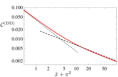
Figure 6: (Color online) Solid line: Double-logarithmic plot of the specific-heat scaling function $\mathcal{C}^{\text{(DD)}}({\tilde{x}})$, (160), of the Gaussian model with DD b.c. in three dimensions as a function of ${\tilde{x}}+\pi^{2}$, with ${\tilde{x}}=t(L/\xi_{0})^{2}$, $t=(T-T_{\text{c}})/T_{\text{c}}$. Dotted: asymptotic behavior at small ${\tilde{x}}+\pi^{2}>0$ according to (161) and (162a), displaying the divergent critical behavior near $T_{\text{c,film}}(L)<T_{\text{c}}$ with an exponent $\alpha=1$. Dashed: asymptotic behavior at large ${\tilde{x}}$ according to (161c) and (162c), displaying the three-dimensional bulk critical behavior above bulk $T_{\text{c}}$ with an exponent $\alpha=1/2$. Near ${\tilde{x}}=0$ corresponding to bulk $T_{\text{c}}$, $\mathcal{C}^{\text{(DD)}}({\tilde{x}})$ is an analytic function with the finite amplitude $\mathcal{C}^{\text{(DD)}}(0)=1/(48\pi)$.

Appendix A Film Thickness

Here we derive the expression (48) for the thickness $\bar{L}$ of the transformed isotropic film. This thickness is given by $L$ times the height of the $d$-dimensional parallelepiped spanned by the transforms $\bm{\hat{x}}_{i}^{\prime}\equiv\bm{\lambda}^{-1/2}\bm{U}\bm{\hat{x}}_{i}$ of the orthogonal unit vectors $\bm{\hat{x}}_{i}$, $i=1,\ldots,d$ over the surface given by the $(d{-}1)$-dimensional parallelepiped spanned by $\bm{\hat{x}}_{i}^{\prime}$, $i=1,\ldots,d{-}1$. Since the volume of a parallelepiped is given by the product of one of its surface areas and the corresponding height, we may write

$$\bar{L}=(V_{d}/V_{d-1})L,$$ (163)

where the volume of the $d$-dimensional parallelepiped has been denoted by $V_{d}$ and the surface area is given by the volume $V_{d-1}$ of the $(d{-}1)$-dimensional parallelepiped. The $m$-dimensional volume $V_{m}$ of a parallelepiped spanned by the $m$ vectors $\vec{v}_{1}$,…,$\vec{v}_{m}$ in an $n$-dimensional space with $n\geq m$ is given by $V_{m}=\left(\det\bm{V}^{T}\bm{V}\right)^{1/2}$, where $\bm{V}$ is the $n\times m$ matrix whose columns are the vectors $\vec{v}_{1}$,…,$\vec{v}_{m}$. Thus we obtain

$$V_{d} =\left[\det(\bm{\lambda}^{-1/2}\bm{U})^{T}(\bm{\lambda}^{-1/2}\bm{U})\right]^{1/2}=\left(\det{\bm{\lambda}}^{-1}\right)^{1/2}$$

$$=\prod_{i=1}^{d}\lambda_{i}^{-1/2}=\left(\det{\bm{A}}^{-1}\right)^{1/2},$$ (164)

where ${\bm{A}}^{-1}$ may also be written as

$${\bm{A}}^{-1}=\left(\begin{array}[]{ccc}\bm{\hat{x}}_{1}^{\prime}\cdot\bm{\hat{x}}_{1}^{\prime}&\cdots&\bm{\hat{x}}_{1}^{\prime}\cdot\bm{\hat{x}}_{d}^{\prime}\\ \vdots&\ddots&\vdots\\ \bm{\hat{x}}_{d}^{\prime}\cdot\bm{\hat{x}}_{1}^{\prime}&\cdots&\bm{\hat{x}}_{d}^{\prime}\cdot\bm{\hat{x}}_{d}^{\prime}\end{array}\right),$$ (168)

and

$$V_{d-1}=\left(\det[\bm{\lambda}^{-1/2}\bm{U}]^{T}[\bm{\lambda}^{-1/2}\bm{U}]\right)^{1/2}$$

$$~{}=\left(\det[\bm{A}^{-1/2}]^{T}[\bm{A}^{-1/2}]\right)^{1/2}=\left(\det[[\bm{A}^{-1}]]\right)^{1/2},$$ (169)

where $[\bm{\lambda}^{-1/2}\bm{U}]$ and $[\bm{A}^{-1/2}]$ are the $d\times(d{-}1)$ matrices that result from removing the last column from the matrices $\bm{\lambda}^{-1/2}\bm{U}$ and $\bm{A}^{-1/2}$, respectively, and where $[[\bm{A}^{-1}]]$ is the $(d{-}1)\times(d{-}1)$ left upper part of ${\bm{A}}^{-1}$. Combining (163), (A), and (A) gives (48).

For the special case where $\bm{A}$ is diagonal, we obtain $V_{d}=\prod_{i=1}^{d}A_{ii}^{-1/2}$ and $V_{d-1}=\prod_{i=1}^{d-1}A_{ii}^{-1/2}$ and thus $V_{d}/V_{d-1}=A_{dd}^{-1/2}$.

Appendix B Free energy

Here we derive $f_{s}(t,L)$ of the Gaussian lattice model in $1<d<4$ dimensions for film geometry with the various b.c. for both the isotropic case and the anisotropic case.

While we follow in spirit the derivation given for DD b.c. in ChDo03 , two simplifications arise: (i) In ChDo03 a slab geometry was investigated, of which the film geometry is only a limiting case; (ii) we perform an exact separation of the surface contributions at an early stage of the calculation and reduce the remaining computations for all b.c. to the case of periodic b.c..

First we consider the isotropic case. We start from (II.1) and (II.1) and use $\ln z=\int_{0}^{\infty}dyy^{-1}\left(e^{-y}-e^{-yz}\right)$ to write the excess free energy as

$$f_{\text{ex}}(t,L) =\frac{1}{2\tilde{a}^{d}}\int_{0}^{\infty}\frac{dy}{y}e^{-y\tilde{r}_{0}/2}B(y)^{d-1}\Delta B_{N}(y),$$ (170)

with $\tilde{r}_{0}$ defined after Eq. (31),

$$\Delta B_{N}(y)\equiv B(y)-B_{N}(y),$$ (171)

$$B(y) =\frac{1}{2\pi}\int_{0}^{2\pi}d\varphi\,\exp[-y(1-\cos\varphi)],$$ (172)

$$B_{N}(y) =\frac{1}{N}\sum_{q_{m}}\exp[-y(1-\cos q_{m}\tilde{a})],$$ (173)

where the sum $\sum_{q_{m}}$ runs over the wave numbers given in (4). The quantity $B(y)\equiv\lim_{N\to\infty}B_{N}(y)$ in (172) is identical to $B(y)$ from (33). By rearranging the sums it is possible to express $B_{N}^{\text{(a)}}(y)$, $B_{N}^{\text{(NN)}}(y)$, $B_{N}^{\text{(DD)}}(y)$, and $B_{N}^{\text{(ND)}}(y)$ in terms of $B_{N}^{\text{(p)}}(y)$. For example, for DD b.c.

$$B_{N}^{\text{(DD)}}(y)$$

$$=\frac{1}{2N}\left(\sum_{m=0}^{N-1}{+}\sum_{m=N+1}^{2N}\right)\exp\left[-y\left(1{-}\cos\frac{\pi(m{+}1)}{N{+}1}\right)\right]$$

$$=-\frac{1+e^{-2y}}{2N}+\frac{N+1}{N}B_{2(N+1)}^{\text{(p)}}(y),$$ (174)

where in the first step we have exploited the symmetry of the cosine about $\pi$, while in the second step $m=-1$ and $m=N$ terms have been added to and subtracted from the sum and subsequently $m$ has been renamed $m-1$. Similar rearrangements can be performed for the other nonperiodic b.c. and we obtain the exact relations

$$\Delta B_{N}^{\text{(a)}}(y) =2\Delta B_{2N}^{\text{(p)}}(y)-\Delta B_{N}^{\text{(p)}}(y),$$ (175a)

$$\Delta B_{N}^{\text{(NN)}}(y) =\frac{e^{-2y}-1}{2N}+\Delta B_{2N}^{\text{(p)}}(y),$$ (175b)

$$\Delta B_{N}^{\text{(DD)}}(y) =\frac{1{+}e^{-2y}{-}2B(y)}{2N}+\left(1{+}\frac{1}{N}\right)\Delta B_{2(N+1)}^{\text{(p)}}(y),$$ (175c)

$$\Delta B_{N}^{\text{(ND)}}(y) =\frac{e^{-2y}-B(y)}{2N}+\left(1+\frac{1}{2N}\right)\Delta B_{2N+1}^{\text{(a)}}(y).$$ (175d)

This leads to the exact representation

$$f_{\text{ex}}(t,L) =\frac{2f_{\text{sf}}(t)}{L}+\frac{1}{2\tilde{a}^{d}}\int_{0}^{\infty}\frac{dy}{y}e^{-y\tilde{r}_{0}/2}B(y)^{d-1}\times$$

$$\Delta B_{N}^{\text{(p)}}(y),$$ periodic b.c., (176a)

$$\Delta B_{N}^{\text{(a)}}(y),$$ antiperiodic b.c., (176b)

$$\Delta B_{2N}^{\text{(p)}}(y),$$ NN b.c., (176c)

$$\left(1+{\textstyle\frac{1}{N}}\right)\Delta B_{2(N+1)}^{\text{(p)}}(y),$$ DD b.c., (176d)

$$\left(1+{\textstyle\frac{1}{2N}}\right)\Delta B_{2N+1}^{\text{(a)}}(y),$$ ND b.c., (176e)

for arbitrary $L=N\tilde{a}$ with $\Delta B_{N}^{\text{(a)}}$ from (175a). For NN, DD, and ND b.c., the surface contribution $2f_{\text{sf}}(t)/L$ originates from the first term on the right hand sides of (175b), (175c), and (175d), respectively. It is given by $f_{\text{sf}}^{\text{(N)}}(t)$, $f_{\text{sf}}^{\text{(D)}}(t)$, and $f_{\text{sf}}^{\text{(ND)}}(t)$ provided in (89) and (14).

The remaining tasks are (i) to determine the large-$N$ behavior of $B_{N}^{\text{(p)}}(y)$ for periodic b.c. and (ii) to translate the result to the other b.c.. For the first task it is useful to distinguish the regimes $0\leq y\lesssim y_{0}$ and $y\gtrsim y_{0}$ in the integral (170), with $y_{0}$ chosen such that $1\ll y_{0}\ll N^{2}$. Thus, for periodic b.c., we separate

$$f_{\text{ex}}(t,L)=\frac{1}{2\tilde{a}^{d}}(f_{1}+f_{2}),$$ (177)

$$f_{1,2}=\int_{1,2}\frac{dy}{y}e^{-y\tilde{r}_{0}/2}B(y)^{d-1}\Delta B_{N}^{\text{(p)}}(y),$$ (178)

with $\int_{1}\equiv\int_{0}^{y_{0}}$ and $\int_{2}\equiv\int_{y_{0}}^{\infty}$, corresponding to (A10) and (A11) of ChDo03 . As shown in (A12)–(A17) of ChDo03 , the large-$N$ dependence of $\Delta B_{N}^{\text{(p)}}(y)$ in the regime $0\leq y\lesssim y_{0}$ is of $O(e^{-N})$, thus $f_{1}$ yields only exponentially small contributions.

Now consider $y\gtrsim y_{0}$ with $y_{0}\gg 1$. Rewrite the sum over $q_{m}$ in (173) for periodic b.c. by letting $m$ run over $m=-N/2,\ldots,N/2-1$ for even $N$ and $m=-(N-1)/2,\ldots,(N-1)/2$ for odd $N$. Then only $|q_{m}\tilde{a}|\ll 1$ can lead to contributions to $B_{N}^{\text{(p)}}(y)$ in (173) that are not exponentially small and we may expand

$$\exp [-y(1-\cos q_{m}\tilde{a})]$$

$$=\exp\left\{-{\textstyle\frac{1}{2}}y(q_{m}\tilde{a})^{2}\left[1+O((q_{m}\tilde{a})^{2})\right]\right\}.$$ (179)

Correspondingly, we obtain in the regime $y\gtrsim y_{0}$ , apart from exponentially small corrections,

$$B_{N}^{\text{(p)}}(y) \approx\frac{1}{N}\sum_{m=-\infty}^{+\infty}\exp\left[-2y\left({\textstyle\frac{\pi m}{N}}\right)^{2}\right]=\frac{1}{N}K\left(2y({\textstyle\frac{\pi}{N}})^{2}\right).$$ (180)

For the evaluation of $f_{2}$, we use (180) and keep only the first term of

$$B(y)=\frac{1}{\sqrt{2\pi y}}\left[1+O(y^{-1})\right].$$ (181)

Extending the lower integration limit in $f_{2}$ to $0$ leads only to exponentially small corrections. Changing the integration variable according to $z=2y(\pi/N)^{2}$ gives for periodic b.c. the result (II.1) with $\mathcal{G}^{\text{(p)}}({\tilde{x}})$ in (83a). Due to (176b)–(176e), we confirm (II.1) also for the other b.c. under consideration here (the surface terms are absent also for antiperiodic b.c.), with the $\mathcal{G}({\tilde{x}})$ provided in (83b), (IV.2), and (114), with specializations to $d=3$ in (87), (IV.3), and (124).

Now add to $L^{-d}\mathcal{G}({\tilde{x}})$ the bulk singular part of the free energy $f_{\text{b,s}}$ from (20) and, for NN or DD b.c. and $d\neq 3$, the surface singular part from (90) (the corresponding part for ND b.c. vanishes, see Sec. IV.4). Observing (18) with $C_{1}$ given after (19) leads to the scaling functions (79), (IV.2), and (IV.4).

For $d=3$ and NN or DD b.c., we add to $L^{-3}\mathcal{G}({\tilde{x}})$ with $\mathcal{G}({\tilde{x}})$ from (IV.3) the bulk singular part of the free energy $f_{\text{b,s}}$ from (20) with $Y_{3}$ from after (34) and the surface singular part from (101) to obtain the results (103).

Inserting the small-$z$ expansion of $K(z)$ into (83a) with (80) gives

$$\mathcal{G}^{\text{(p)}}({\tilde{x}})$$

$$=-\int_{0}^{\infty}\frac{dz}{\pi}\left(\frac{\pi}{z}\right)^{(d+2)/2}e^{-z{\tilde{x}}/(2\pi)^{2}}\sum_{n=1}^{\infty}e^{-n^{2}\pi^{2}/z}.$$ (182)

For large ${\tilde{x}}$, the right hand side is dominated by the first term of the sum. The remaining integral may be evaluated in a saddle point approximation. This yields, together with (83b), (IV.2), and (114), the exponential decay of the non-surface terms in (85), (IV.2), and (IV.4).

For the anisotropic case, we consider two different couplings $J_{\perp}$ and $J_{\parallel}$, see (51). Then (170) is replaced by

$$f_{\text{ex}}(t,L)$$

$$=\frac{1}{2\tilde{a}^{d}}\int_{0}^{\infty}\frac{dy}{y}e^{-y\tilde{r}_{0,\perp}/2}B((J_{\parallel}/J_{\perp})y)^{d-1}\Delta B_{N}(y),$$ (183)

with $\tilde{r}_{0,\perp}\equiv r_{0}\tilde{a}^{2}/(2J_{\perp})$. For the leading singular finite-size terms only the leading large-$y$ behavior of $B(y)$ given in (181) matters, see the derivation of (83a) for periodic b.c. above and its translation through (176b)–(176e) to the other b.c., manifested in (83b), (IV.2), and (114). The same is true for the leading singular surface terms as may be inferred from the derivation of (90) for $d\neq 3$. Thus the factor $J_{\parallel}/J_{\perp}$ in the argument of $B$ in (B) leads to an additional factor $(J_{\perp}/J_{\parallel})^{(d-1)/2}$ in front of the leading singular contributions to the excess free energy $f_{\text{ex}}(t,L)$. Eqs. (31)–(32) are replaced by

$$f_{\text{b}}(t)=\frac{1}{2\tilde{a}^{d}}\left[\ln\frac{J_{\perp}}{\pi}+\widetilde{W}_{d}(\tilde{r}_{0,\perp},J_{\parallel}/J_{\perp})\right],$$ (184)

$$\widetilde{W}_{d}(z,w)\equiv\int_{0}^{\infty}\frac{dy}{y}\left[e^{-y/2}-e^{-zy/2}B(y)B(wy)^{d-1}\right].$$ (185)

Thus, because of the argument $(J_{\parallel}/J_{\perp})y$ of $B$, the same factor $(J_{\perp}/J_{\parallel})^{(d-1)/2}$ appears in front of the leading singular bulk part. Since the temperature dependence enters only through the parameter $\tilde{r}_{0,\perp}=\tilde{a}^{2}/\xi_{\perp}^{2}$, where $\xi_{\perp}$ is the correlation length (56b), it is straightforward to confirm (II.3) for all b.c. on the basis of these properties.

Appendix C Comparison with Ref. KrDi92a

In Sec. IV we stated the identity of $\mathcal{G}({\tilde{x}})$ with the functions $\Theta_{+}^{(1)}(y_{+})$ used in KrDi92a (as noted for periodic and antiperiodic b.c. after Eq. (83), for NN and DD b.c. after Eq. (IV.2), and for ND b.c. after Eq. (114)). For periodic b.c., this equivalence follows from using the expansion (3.38) in DaKr04 in terms of Bessel functions, which provides another representation of $\mathcal{G}^{\text{(p)}}$. With ${\tilde{x}}=y_{+}^{2}$, we obtain

$$\mathcal{G}^{\text{(p)}}(y_{+}^{2})$$

$$\equiv-\frac{1}{2\pi}\int_{0}^{\infty}dz\,(\pi/z)^{(d+1)/2}e^{-zy_{+}^{2}/(2\pi)^{2}}\left[K(z)-\sqrt{\pi/z}\right]$$

$$=-\frac{1}{\pi}\sum_{n=1}^{\infty}\int_{0}^{\infty}dz(\pi/z)^{d/2+1}e^{-zy_{+}^{2}/(2\pi)^{2}}e^{-n^{2}\pi^{2}/z}$$

$$=-2y_{+}^{d/2}\sum_{n=1}^{\infty}\frac{K_{d/2}(ny_{+})}{(2\pi n)^{d/2}}$$

$$=-\frac{y_{+}^{d}}{(4\pi)^{(d-1)/2}\Gamma(\frac{d+1}{2})}\sum_{n=1}^{\infty}\int_{1}^{\infty}dz(z^{2}-1)^{(d-1)/2}e^{-nzy_{+}}$$

$$=-\frac{y_{+}^{d}}{(4\pi)^{(d-1)/2}\Gamma(\frac{d+1}{2})}\int_{1}^{\infty}dz\frac{(z^{2}-1)^{(d-1)/2}}{e^{zy_{+}}-1}$$

$$\equiv\Theta_{+\text{per}}^{(1)}(y_{+}),$$ (186)

valid for $y_{+}>0$. The other identities between $\mathcal{G}({\tilde{x}})$ and $\Theta_{+}^{(1)}(y_{+})$ follow similarly. They may also be derived by showing the identities (83b), (IV.2), and (114) for the functions $\Theta_{+}^{(1)}$ as represented in KrDi92a .

Appendix D Functions

For $|z|<1$, the polylogarithms are defined by $\operatorname{Li}_{\nu}(z)=\sum_{k=1}^{\infty}z^{k}/k^{\nu}$ and for $|z|\geq 1$ by their analytic continuation. They are analytic in the complex plane except at $z=1$ and except for a branch cut that we take along $z\in]1,\infty[$. We need $\operatorname{Li}_{\nu}(z)$ for $\nu=1,2,3$. Well known relations are $\operatorname{Li}_{\nu}(1)=\zeta(\nu)$ for $\operatorname{Re}\nu>1$, $\operatorname{Li}_{\nu}(-1)=(2^{1-\nu}-1)\zeta(\nu)$, $\operatorname{Li}_{1}(z)=-\ln(1-z)$, and $\operatorname{Li}_{\nu}^{\prime}(z)=\operatorname{Li}_{\nu-1}(z)/z$ for $z\notin[1,\infty[$, where $\zeta(\nu)\equiv\sum_{k=1}^{\infty}k^{-\nu}$ is Riemann’s zeta function. Combining them we may write for $z\geq 0$

$$\operatorname{Li}_{3}(\pm e^{-z}) +z\operatorname{Li}_{2}(\pm e^{-z})$$

$$=\frac{1}{8}(1\pm 7)\zeta(3)+\int_{0}^{z}dx\,x\ln(1\mp e^{-x}),$$ (187)

which is needed for App. E.

The various functions $\mathcal{K}_{d}^{\text{($\tau$)}}$ appearing in (156) read

$$\mathcal{K}_{d}^{\text{(p)}}(y) =-\frac{1}{32\pi^{3}}\int_{0}^{\infty}dz\left(\pi/z\right)^{(d-3)/2}e^{-zy/(2\pi)^{2}}\times$$

$$\phantom{=}\left[K(z)-\sqrt{\pi/z}\right],$$ (188a)

$$\mathcal{K}_{d}^{\text{(a)}}(y) =-\frac{1}{32\pi^{3}}\int_{0}^{\infty}dz\left(\pi/z\right)^{(d-3)/2}e^{-zy/(2\pi)^{2}}\times$$

$$\phantom{=}\left\{e^{z/4}\left[K(z/4)-K(z)\right]-\sqrt{\pi/z}\right\},$$ (188b)

$$\mathcal{K}_{d}^{\text{(DD)}}(y) =-\frac{1}{2^{d+1}\pi^{3}}\int_{0}^{\infty}dz\left(\pi/z\right)^{(d-3)/2}e^{-zy/\pi^{2}}\times$$

$$\phantom{=}\left\{e^{z}[K(z)-1]-\sqrt{\pi/z}+1\right\}.$$ (188c)

and $\mathcal{K}_{d}^{\text{(NN)}}(y)=2^{4-d}\mathcal{K}_{d}^{\text{(p)}}(4y)$, $\mathcal{K}_{d}^{\text{(ND)}}(y)=2^{4-d}\mathcal{K}_{d}^{\text{(a)}}(4y)$.

Appendix E Analyticity properties

Here we show that the $d=3$ expressions (86b) for $\mathcal{F}^{\text{(a)}}({\tilde{x}})$ and (108) for $L^{3}f_{\text{s}}^{\text{(DD)}}(t,L)+(8\pi)^{-1}{\tilde{x}}\ln(L/\tilde{a})$ are analytic for ${\tilde{x}}>-\pi^{2}$ and are finite and real at ${\tilde{x}}=-\pi^{2}$. Combining (87b) and (D), we obtain for ${\tilde{x}}\geq 0$

$$\mathcal{G}^{\text{(a)}}({\tilde{x}})=-\frac{1}{2\pi}\left[-\frac{3}{4}\zeta(3)+\int_{0}^{\sqrt{{\tilde{x}}}}dzz\ln(1+e^{-z})\right]$$

$$=\frac{1}{4\pi}\left\{\frac{3}{2}\zeta(3)+\frac{1}{3}{\tilde{x}}^{3/2}-\int_{0}^{\tilde{x}}d{\tilde{x}}^{\prime}\ln\left[2\cosh(\sqrt{{\tilde{x}}^{\prime}}/2)\right]\right\}.$$ (189)

Since $\cosh(\sqrt{{\tilde{x}}^{\prime}})$ is analytic and positive at ${\tilde{x}}^{\prime}=0$, the analytic continuation of $\mathcal{F}^{\text{(a)}}({\tilde{x}})$ in (86b) from positive ${\tilde{x}}$ to other ${\tilde{x}}$ is analytic at ${\tilde{x}}=0$. Inspection of (E) shows that the integral there is also analytic for all other ${\tilde{x}}>-\pi^{2}$. Thus (86b) is analytic in ${\tilde{x}}$ for all ${\tilde{x}}>-\pi^{2}$. Computing the integral in (E) for ${\tilde{x}}=-\pi^{2}$ and combining the result with (86b) gives the result (88). Combining (IV.3) and (D), we obtain for ${\tilde{x}}\geq 0$

$$\mathcal{G}^{\text{(DD)}}({\tilde{x}}) =-\frac{1}{16\pi}\left[\zeta(3)+\int_{0}^{2\sqrt{{\tilde{x}}}}dzz\ln(1-e^{-z})\right]$$

$$=-\frac{1}{16\pi}\Bigg{[}\zeta(3)-\frac{4}{3}{\tilde{x}}^{3/2}+{\tilde{x}}(\ln{\tilde{x}}-1)$$

$$\hskip 40.0pt+2\int_{0}^{\tilde{x}}d{\tilde{x}}^{\prime}\ln\frac{2\sinh(\sqrt{{\tilde{x}}^{\prime}})}{\sqrt{{\tilde{x}}^{\prime}}}\Bigg{]}.$$ (190)

Since $\sinh(\sqrt{{\tilde{x}}^{\prime}})/\sqrt{{\tilde{x}}^{\prime}}$ is analytic and positive at ${\tilde{x}}^{\prime}=0$, the analytic continuation of (108) is analytic at ${\tilde{x}}=0$. The integral in (E) is also analytic for all other ${\tilde{x}}>-\pi^{2}$. Thus (108) is analytic in ${\tilde{x}}$ for all ${\tilde{x}}>-\pi^{2}$. Using (E) to expand (108) around ${\tilde{x}}=-\pi^{2}$ for ${\tilde{x}}\geq-\pi^{2}$ gives (IV.3), with a finite value of (108) at ${\tilde{x}}=-\pi^{2}$.

References

- (1) F.M. Gasparini, M.O. Kimball, K.P. Mooney, and M. Diaz-Avila, Rev. Mod. Phys. 80, 1009 (2008).
- (2) R. Garcia and M.H.W. Chan, Phys. Rev. Lett. 83, 1187 (1999); A. Ganshin, S. Scheidemantel, R. Garcia, and M.H.W. Chan, Phys. Rev. Lett. 97, 075301 (2006).
- (3) M. Fukuto, Y.F. Yano, and P.S. Pershan, Phys. Rev. Lett. 94, 135702 (2005).
- (4) N. Schultka and E. Manousakis, J. Low Temp. Phys. 111, 783 (1998); M. Hasenbusch, arXiv:0904.1535v1; arXiv:0905.2096v1; arXiv:0907.2847v1.
- (5) A. Hucht, Phys. Rev. Lett. 99, 185301 (2007); O. Vasilyev, A. Gambassi, A. Maciołek, and S. Dietrich, Europhys. Lett. 80, 60009 (2007).
- (6) O. Vasilyev, A. Gambassi, A. Maciołek, and S. Dietrich, Phys. Rev. E 79, 041142 (2009); 80, 039902(E) (2009).
- (7) W. Huhn and V. Dohm, Phys. Rev. Lett. 61, 1368 (1988); R. Schmolke, A. Wacker, V. Dohm, and D. Frank, Physica B 165&166, 575 (1990).
- (8) M. Krech and S. Dietrich, Phys. Rev. A 46, 1886 (1992).
- (9) M. Krech and S. Dietrich, Phys. Rev. A 46, 1922 (1992).
- (10) For reviews see M. Krech, The Casimir Effect in Critical Systems (World Scientific, Singapore, 1994); J. Phys.: Condens. Matter 11, R391, (1999).
- (11) V. Dohm, Phys. Scr. T 49, 46 (1993); U. Mohr and V. Dohm, Physica B 284-288, 43 (2000).
- (12) P. Sutter and V. Dohm, Physica B 194-196, 613 (1994).
- (13) M. Töpler and V. Dohm, Physica B 329-333, 200 (2003).
- (14) H.W. Diehl, D. Grüneberg, and M.A. Shpot, Europhys. Lett. 75, 241 (2006).
- (15) D. Grüneberg and H.W. Diehl, Phys. Rev. B 77, 115409 (2008).
- (16) Z. Borjan and P.J. Upton, Phys. Rev. Lett. 81, 4911 (1998); 101, 125702 (2008).
- (17) V. Dohm, Europhys. Lett. 86, 20001 (2009).
- (18) R. Zandi, J. Rudnick, and M. Kardar, Phys. Rev. Lett. 93, 155302 (2004); R. Zandi, A. Shackell, J. Rudnick, M. Kardar, and L.P. Chayes, Phys. Rev. E 76, 030601(R) (2007); A. Maciołek, A. Gambassi, and S. Dietrich, Phys. Rev. E 76, 031124 (2007).
- (19) D. Frank and V. Dohm, Phys. Rev. Lett. 62, 1864 (1989); Physica B 165&166, 543 (1990); Z. Phys. B: Condens. Matter 84, 443 (1991).
- (20) J.O. Indekeu, M.P. Nightingale, and W.V. Wang, Phys. Rev. B 34, 330 (1986).
- (21) V. Privman, in Finite Size Scaling and Numerical Simulation of Statistical Systems, edited by V. Privman (World Scientific, Singapore, 1990), p. 1.
- (22) V. Privman, A. Aharony, and P.C. Hohenberg, in Phase Transitions and Critical Phenomena, edited by C. Domb and J.L. Lebowitz (Academic, N.Y., 1991), Vol. 14, p. 1.
- (23) R. Evans and J. Stecki, Phys. Rev. B 49, 8842 (1994).
- (24) J. Rudnick, R. Zandi, A. Shackell, and D. Abraham, arXiv:1001.0994v1.
- (25) M.N. Barber and M.E. Fisher, Ann. Phys. (N.Y.) 77, 1 (1973).
- (26) J.G. Brankov, D.M. Dantchev, and N.S. Tonchev, Theory of Critical Phenomena in Finite-Size Sytems - Scaling and Quantum Effects (World Scientific, Singapore, 2000).
- (27) B. Kastening and V. Dohm, in Path Integrals, New Trends and Perspectives, Proc. Int. Conf., edited by W. Janke and A. Pelster (World Scientific, Singapore, 2008), p. 283.
- (28) E. Brézin, Ann. N.Y. Acad. Sci. 410, 339 (1983).
- (29) H. Chamati, J. Phys. A 41, 375002 (2008).
- (30) J.L. Cardy, in Finite-Size Scaling, edited by J.L. Cardy (North Holland, Amsterdam, 1988), p. 1.
- (31) X.S. Chen and V. Dohm, Phys. Rev. E 67, 056127 (2003).
- (32) H.J. Krause, R. Schloms, and V. Dohm, Z. Phys. B: Condens. Matter 79, 287 (1990); S.A. Larin, M. Mönnigmann, M. Strösser, and V. Dohm, Phys. Rev. B 58, 3394 (1998).
- (33) V. Dohm, Z. Phys. B: Condens. Matter 60, 61 (1985); 61, 193 (1985); R. Schloms and V. Dohm, Nucl. Phys. B 328, 639 (1989); Phys. Rev. B 42, 6142 (1990).
- (34) J.A. Nissen, T.C.P. Chui, and J.A. Lipa, J. Low Temp. Phys. 92, 353 (1993).
- (35) D.M. Dantchev and M. Krech, Phys. Rev. E 69, 046119 (2004).
- (36) V. Dohm, Phys. Rev. E 77, 061128 (2008); 79, 049902(E) (2009).
- (37) D. Dantchev, M. Krech, and S. Dietrich, Phys. Rev. E 67, 066120 (2003).
- (38) X.S. Chen and V. Dohm, Phys. Rev. E 70, 056136 (2004).
- (39) V. Dohm, J. Phys. A 39, L259 (2006).
- (40) V. Dohm, Physik Journal 8, 37 (2009).
- (41) D. Dantchev and D. Grüneberg , Phys. Rev. E 79, 041103 (2009).
- (42) W. Selke and L.N. Shchur, J. Phys. A 38, L739 (2005); Phys. Rev. E 80, 042104 (2009).
- (43) D.M. Danchev, J.G. Brankov, and M.E. Amin, J. Phys. A: Math. Gen. 30, 1387 (1997); D.M. Dantchev and J.G. Brankov, J. Phys. A: Math. Gen. 36, 8915 (2003).
- (44) B. Kastening and V. Dohm, in preparation.
- (45) V. Privman, Phys. Rev. B 38, 9261 (1988).
- (46) V. Privman and M.E. Fisher, Phys. Rev. B 30, 322 (1984).
- (47) X.S. Chen and V. Dohm, Eur. Phys. J. B 10, 687 (1999).
- (48) D. Dantchev and J. Rudnick,, Eur. Phys. J. B 21, 251 (2001).
- (49) V. Privman and J. Rudnick, J. Phys. A: Math. Gen. 19, L 1215 (1986).
- (50) H.W. Diehl and H. Chamati, Phys. Rev. B 79, 104301 (2009).
- (51) I.S. Gradshteyn and I.M. Ryzhik, Table of Integrals, Series, and Products, Fifth Edition (Academic, N.Y., 1994).
- (52) In our Sec. VI, the quantities , , and denote the asymptotic amplitudes of the exponential (“true”) bulk correlation lengths above of the two-dimensional Ising model as employed in Ref. [20] and in H. Au-Yang and M.E. Fisher, Phys. Rev. B 11, 3469 (1975). For the relation between exponential and second-moment bulk correlation lengths see M.E. Fisher and R.J. Burford, Phys. Rev. 156, 583 (1967), H.B. Tarko and M.E. Fisher, Phys. Rev. Lett. 31, 926 (1975), G. Flöter and S. Dietrich, Z. Phys. B: Condens. Matter 97, 213 (1995), G. Delfino, Phys. Lett. B 419, 291 (1998), and X.S. Chen and V. Dohm, Eur. Phys. J. B 15, 283 (2000). Also in the comment after Eq. (40) in our Sec. II, the quantity denotes the asymptotic amplitude of the exponential bulk correlation length above of the two-dimensional Ising model.