Coagulation reactions in low dimensions: Revisiting subdiffusive $A+A$ reactions in one dimension

Abstract

We present a theory for the coagulation reaction $A+A\to A$ for particles moving subdiffusively in one dimension. Our theory is tested against numerical simulations of the concentration of $A$ particles as a function of time (“anomalous kinetics”) and of the interparticle distribution function as a function of interparticle distance and time. We find that the theory captures the correct behavior asymptotically and also at early times, and that it does so whether the particles are nearly diffusive or very subdiffusive. We find that, as in the normal diffusion problem, an interparticle gap responsible for the anomalous kinetics develops and grows with time. This corrects an earlier claim to the contrary on our part.

I Introduction

The traditional laws of mass action that describe the time evolution of the macroscopic global concentrations of reactants and products in chemical reactions assume that the system is well stirred and therefore spatially homogeneous. However, there are many situations when a reactive system is not well mixed; in that case one must deal with local concentrations and account for the effects of spatial inhomogeneities on local reaction rates. Spatial variations in concentrations of reactants lead to changes (often called “anomalies”) in the time dependences of the spatially averaged macroscopic concentrations. One often encounters this situation when diffusion is the only mixing mechanism, particularly when diffusion is the rate limiting step for a reaction to occur. The inefficiency of diffusion as a mixing mechanism becomes more pronounced with decreasing dimensionality of the system, and it is therefore commonly accepted that diffusion-limited reactions in constrained geometries exhibit kinetic “anomalies” Kotomin . An exact description of diffusion-limited reactions in the face of nonuniform spatial distributions of reactants typically requires an infinite hierarchy of correlation functions to properly incorporate spatial correlations. In practice, such hierarchies are often truncated at the first or second level, giving rise to well-known reaction-diffusion equations whose solutions are sometimes fairly satisfactory (and sometimes not) in capturing the principal deviations form the laws of mass action Something1 ; Something2 .

The judgment as to the success or failure of approximate reaction-diffusion models has mostly relied on comparisons with numerical simulations. There has always been a quest for exact analytic solutions against which approximate reaction-diffusion theories could be tested, but there have been very few successes, among them the coagulation ($A+A\to A$ and $A+A\rightleftharpoons A$) and annihilation ($A+A\to 0$) reactions Something2 ; Something3 . Exact solutions in these cases have been possible because, if instead of focusing on the concentration of reactants, one focuses on the evolution of empty intervals (coagulation reactions) or on the number parity (even or odd) of particles in an interval (annihilation reactions), one arrives at exactly linear diffusion equations. These solutions have provided a wealth of information against which to measure the approximate solutions obtained from more standard approaches for these particular reactions. Unfortunately, the interval approaches are not generalizable to other reactions.

In the past few years there have also been attempts to understand chemical reactions in low dimensions when the reactants move subdiffusively. This has been a particularly interesting subject in view of the many systems, mainly biological, in which such reactions occur in a complex or constrained environment that does not even permit ordinary diffusive motion of chemical species. All the difficulties encountered in diffusive systems are exacerbated in this case because motions are even slower, a fact that turns out to have profound consequences on spatial as well as temporal correlations ourlatest and to cause much greater difficulties in both numerical simulations and analytic attempts. One approach to this problem has been to essentially adapt the existing reaction-diffusion models by modifying the diffusive description to a subdiffusive one involving fractional diffusion operators. These descriptions are phenomenological in nature, and much work remains to be done to understand how one might arrive at a mesoscopic description from microscopic considerations. In particular, there are many questions about how to describe the reaction terms in subdiffusive systems, and there is clear evidence that the problem is usually not even separable into a simple sum of a term describing the motion of the particles and one describing the reaction.

The subdiffusive coagulation and annihilation problems seemed to offer a parallel opportunity for exact solution if one again concentrated on the properties of intervals. We followed this route in our earlier work ourold , and formulated what we thought to be exact subdiffusive equations for the intervals from whose solution one could calculate the particle concentrations and interparticle separations, as had been done in the diffusive problem. These solutions led us to the conclusion that interparticle gaps do not occur in the subiffusive problem, a result that seemed reasonable for particles that move sufficiently slowly. However, subsequent numerical simulations indicated that a gap does develop no matter how subdiffusive the particles, and this led to a reassessment of the assumptions of our original theory. In this paper we present this numerical evidence, a description of the difficulty with the original theory, and a new theory which, albeit still approximate, seems to capture the correct behavior to a very high degree of accuracy. Also, we recently developed a mean field theory for this problem ourlatest but it is only valid for dimension 3 and higher. We concentrate on the coagulation problem, although a similar approach may be helpful for the annihilation reaction.

In Sec. II we describe the difficulties with our previous 1D theory ourold . Section III presents our new theory. Section IV discusses some special interesting issues that arise in this problem, and in Sec. V we present the numerical evidence to support our theory. We conclude with a summary in Sec. VI.

II Traditional Theory

The interparticle distribution function method focuses on the “empty interval” function $E(x,t)$, defined as the probability that an interval of length $x$ is empty of particles at time $t$. From $E(x,t)$ one obtains the concentration of particles,

$$c(t)=-\left.\frac{\partial E(x,t)}{\partial x}\right|_{x=0},$$ (1)

and the interparticle distribution function,

$$p(x,t)=\frac{1}{c(t)}\frac{\partial^{2}E(x,t)}{\partial x^{2}},$$ (2)

which is the probability density that the first $A$ to be found to one side of a given $A$ at time $t$ is a distance $x$ away. The question of interest is how to determine the empty interval function.

If the particles undergo normal diffusion, the probability density for finding a particle $A$ at $y$ at time $t$ in the absence of reactions obeys the diffusion equation

$$\frac{\partial}{\partial t}P(y,t)=D\frac{\partial^{2}}{\partial y^{2}}P(y,t).$$ (3)

In the presence of the coagulation reaction, the empty interval function focuses on the diffusive motion of the particles at each end of an empty interval and one readily arrives at the exact equation

$$\frac{\partial}{\partial t}E(x,t)=2D\frac{\partial^{2}}{\partial x^{2}}E(x,t).$$ (4)

The equation is easily understood from the fact that the empty interval dynamics is the same as that of the individual particles but with double the diffusion coefficient to reflect the relative motion of two diffusive particles. This readily tractable equation, together with appropriate boundary conditions, exactly solves the diffusive $A+A\to A$ problem in one dimension.

A standard approach for the description of subiffusive processes starts from the continuous time random walk (CTRW) formalism, in which a walker jumps from one site on a lattice to another in consecutive steps as time proceeds MetKlaPhysRep ; Hughes1 . Both the jump distances $n$ and times $t$ between jumps are random variables drawn from a probability distribution function $\phi(n,t)$. If the jump distances and jump times are independent random variables, then this distribution function is simply a product, $\phi(n,t)=w(n)\psi(t)$. ”Normal“ CTRWs are associated with distributions $w(n)$ and $\psi(t)$ that have finite first moments, and the scaling limit that leads from the random walk to the diffusion equation is well known. One way to obtain a subdiffusive process is for the waiting time distribution $\psi(t)$ to be heavy-tailed, i.e., $\psi(t)\sim t^{-1-\gamma}$ with $0<\gamma<1$ for long times, so that the mean waiting time between jumps diverges. In this case a number of scaling approaches can be found in the literature, with a particularly helpful discussion in Scalas . In the absence of reactions, in the continuum limit with a particular scaling one arrives at a “fractional diffusion equation” for the evolution of the probability density $P(y,t)$ of a subdiffusive particle,

$$\frac{\partial}{\partial t}P(y,t)=~{}_{0}D_{t}^{1-\alpha}K_{\alpha}\frac{\partial^{2}}{\partial y^{2}}P(y,t),$$ (5)

where $~{}_{0}D_{t}^{1-\alpha}$ is the Riemann-Liouville operator,

$$~{}_{0}D_{t}^{1-\alpha}P(y,t)=\frac{1}{\Gamma(\alpha)}\frac{\partial}{\partial t}\int_{0}^{t}d\tau\frac{P(y,\tau)}{(t-\tau)^{1-\alpha}},$$ (6)

and $K_{\alpha}$ is the generalized diffusion coefficient. The mean square displacement of the $A$ particle for large $t$ that follows from this evolution equation is

$$\langle y^{2}(t)\rangle\sim\frac{2K_{\alpha}}{\Gamma(1+\alpha)}t^{\alpha},$$ (7)

which reduces to the ordinary diffusion result when $\alpha=1$ ($K_{1}=D$). In our earlier work we argued that the same reasoning that led from Eq. (3) to Eq. (4) would also lead from Eq. (5) to the interval equation

$$\frac{\partial}{\partial t}E(x,t)=~{}_{0}D_{t}^{1-\alpha}2K_{\alpha}\frac{\partial^{2}}{\partial x^{2}}E(x,t),$$ (8)

and then calculated the particle concentration and interparticle distribution function from the solution of this equation with appropriate boundary conditions.

The difficulty with this reasoning is the fact that in the subdiffusive problem we must face the issue of aging Barkai , which we have not done above. To describe the issue, we again turn to a CTRW point of view of the problem. Consider first the diffusion problem, where the continuum limit leads to a diffusion equation. In this limit, in which the mean time between steps and the step length go to zero in an appropriate way, one arrives at the diffusion equation. In particular, in the diffusive problem the steps are sufficiently frequent that one need not keep track of extremely long sojourns of a particle at any one site, and what transpired in the past is quickly forgotten. A similar formulation of the subdiffusive problem involves waiting time distributions with an infinite mean time between steps. Even worse, because of aging, the waiting time distribution for a particle to take its next step at time $t$ having arrived at its current location at time $t^{\prime}$ is no longer simply a function of the difference $t-t^{\prime}$ but of each time separately. To understand the effects of these complications, suppose that an observer looks at the system at time $t$ and sees an empty interval of size $x$ at that instant. For normally diffusive particles, the evolution of the size of this interval does not depend on the time at which the interval was first created. However, in order to predict the evolution of this gap for subdiffusive particles the observer must know how long each of the two particles at the ends of this interval have been at that location. Due to aging, the evolution depends on the times $t-t_{l}$ and $t-t_{r}$, where $t_{l}$ and $t_{r}$ are the times at which the left and right particles jumped to the locations seen by the observer at time $t$. Moreover, even if the two particles arrived at this location at the same time, i.e., $t_{l}=t_{r}$, the shortening and lengthening of this gap is not correctly described by Eq. (8),as we will show in Sec. III [cf. Eqs. (9)-(17)].

III Theory Revisited

To find a more appropriate description for the evolution of the empty interval, we introduce two hypotheses. As we state each hypothesis, we provide an argument as to its approximate nature.

We start by forgetting the reaction for a moment, and simply consider the motion of (mutually transparent) $A$ particles on an infinite line. We define ${\mathcal{P}}_{\alpha}(x,t)$ as the probability density for $x$ to be the distance between two subdiffusive particles at time $t$ with the initial condition ${\mathcal{P}}_{\alpha}(x,0)=\delta(x)$, i.e.,

$$\mathcal{P}_{\alpha}(x,t)=\int_{-\infty}^{\infty}dyP_{\alpha}(x-y,t)P_{\alpha}(y,t).$$ (9)

Here $P_{\alpha}(y,t)$ is the propagator of the subdiffusion equation, i.e., the solution of Eq. (5) with the initial condition $P_{\alpha}(y,0)=\delta(y)$. In Fourier space the solution in closed form is the Mittag-Leffler function,

$$\tilde{P}_{\alpha}(q,t)=E_{\alpha}(-K_{\alpha}q^{2}t^{\alpha}).$$ (10)

The Fourier transform of Eq. (9) then tells us that

$$\mathcal{\tilde{P}}_{\alpha}(q,t)=\left(\tilde{P}_{\alpha}(q,t)\right)^{2}=\left[E_{\alpha}(-K_{\alpha}q^{2}t^{\alpha})\right]^{2},$$ (11)

and correspondingly,

$$\mathcal{P}_{\alpha}(y,t) = \frac{1}{2\pi}\int_{-\infty}^{\infty}dqe^{-iqy}\left[E_{\alpha}(-K_{\alpha}q^{2}t^{\alpha})\right]^{2}$$ (12)

$$= \frac{1}{\pi}\int_{0}^{\infty}dq\cos(qy)\left[E_{\alpha}(-K_{\alpha}q^{2}t^{\alpha})\right]^{2}.$$

We do not know the evolution equation for ${\mathcal{P}}_{\alpha}(x,t)$, i.e., we do not know the operator $\mathfrak{F}_{\alpha}$ such that $\mathfrak{F}_{\alpha}{\mathcal{P}}_{\alpha}(x,t)=0$, except for $\alpha=1$. In this case the Mittag-Leffler function reduces to an exponential, $E_{1}(-z)=\exp(-z)$, so that $\mathcal{\tilde{P}}_{1}(q,t)=\exp(-2K_{1}q^{2}t)$ and the corresponding function $\mathcal{P}_{1}(x,t)$ is the solution of the diffusion equation (3) but with double the diffusion coefficient,

$$\frac{\partial}{\partial t}\mathcal{P}_{1}(x,t)=2D\frac{\partial^{2}}{\partial x^{2}}\mathcal{P}_{1}(x,t),$$ (13)

with $K_{1}\equiv D$. However, for $\alpha<1$ the Fourier transform of the solution of the subdiffusion equation with double the subdiffusion coefficient,

$$\frac{\partial}{\partial t}\mathcal{Q}_{\alpha}(x,t)\;=\;_{0}D_{t}^{1-\alpha}\;2K_{\alpha}\frac{\partial^{2}}{\partial x^{2}}\mathcal{Q}_{\alpha}(x,t),$$ (14)

is the Mittag-Leffler function of twice the argument in Eq. (10),

$$\tilde{\mathcal{Q}}_{\alpha}(q,t)=E_{\alpha}(-2K_{\alpha}q^{2}t^{\alpha}).$$ (15)

Clearly, except for $\alpha=1$,

$$\left[E_{\alpha}(-K_{\alpha}q^{2}t^{\alpha})\right]^{2}\neq E_{\alpha}(-2K_{\alpha}q^{2}t^{\alpha}),$$ (16)

so that $\mathcal{P}_{\alpha}\neq\mathcal{Q}_{\alpha}$, and the operator $\mathfrak{F}_{\alpha}$ is not straightforwardly obtained from the subdiffusion equation,

$$\mathfrak{F}_{\alpha}\neq\frac{\partial}{\partial t}\;-\;_{0}D_{t}^{1-\alpha}\;2K_{\alpha}\frac{\partial^{2}}{\partial x^{2}}.$$ (17)

III.1 Hypothesis 1

The central hypothesis of our new theory is that the (unknown) equation that describes the evolution of ${\mathcal{P}}_{\alpha}(x,t)$ is the same as the equation that describes the evolution of the empty interval function $E(x,t)$, i.e., that

$$\mathfrak{F}_{\alpha}E(x,t)=0,\qquad 0\leq x<\infty$$ (18)

This hypothesis is in general an approximation because the distribution of particles is not expected to be the same in the presence and absence of the reaction (although in higher dimensions it is ourlatest ). While there is no memory of prior reaction events in the diffusive problem, in the subdiffusive case this memory persists and may lead to a distortion of the distribution relative to that of the particles when there is no reaction. We only know how to assess the severity of this approximation via comparison of results with numerical simulations ourlatest (see Sec. V).

How does this hypothesis help us find the empty interval distribution when in fact we do not know the operator $\mathfrak{F}_{\alpha}$? It helps us because we know the solution ${\mathcal{P}}_{\alpha}(x,t)$, which is then the Green function or propagator for the empty interval distribution. In other words, while we do not know the equation of evolution for $E(x,t)$, we have sufficient information to construct the function $E(x,t)$ itself explicitly. The interval function is subject to the additional conditions

$$E(0,t) =1,$$ (19)

$$E(\infty,t) =0$$

$$E(x,0) =f(x).$$

The first boundary condition is the probability that an interval of vanishing width is empty. As in the diffusive problem, this probability must be unity. The second simply recognizes the existence of particles at any time $t$, and the third is determined by the initial distribution of empty intervals.

In order to construct the solution $E(x,t)$ from our knowledge of the propagator $\mathcal{P}_{\alpha}(x,t)$, we introduce our second hypothesis.

III.2 Hypothesis 2

The second hypothesis of our theory is that the operator $\mathfrak{F}_{\alpha}$ is linear. We know this operator to be linear when $\alpha=1$, but it is most likely an approximation when $\alpha<1$, although our lack of information about $\mathfrak{F}_{\alpha}$ makes it difficult to assess. While evolution equations describing various quantities in some other reaction-subdiffusion problems are in fact not linear, the connection between those systems and the one considered here is not clear.

In any case, under this hypothesis we can split $E(x,t)$ into two parts, each of which satisfies conditions whose symmetry properties allow for the advantageous use of our knowledge of the propagator. In particular, we write

$$E(x,t)=E^{\mathcal{T}}(x,t)+E^{\mathcal{A}}(x,t),$$ (20)

where the individual pieces satisfy the following:

$$\mathfrak{F}_{\alpha}E^{\mathcal{T}}(x,t) =0,\qquad 0\leq x<\infty$$ (21)

$$E^{\mathcal{T}}(0,t) =0,$$

$$E^{\mathcal{T}}(\infty,t) =0$$

$$E^{\mathcal{T}}(x,0) =f(x)$$

and

$$\mathfrak{F}_{\alpha}E^{\mathcal{A}}(x,t) =0,\qquad 0\leq x<\infty$$ (22)

$$E^{\mathcal{A}}(0,t) =1,$$

$$E^{\mathcal{A}}(\infty,t) =0$$

$$E^{\mathcal{A}}(x,0) =0.$$

The superscripts ${\mathcal{T}}$ and ${\mathcal{A}}$ denote “transient” and “asymptotic,” respectively, for reasons that become evident below.

III.3 Asymptotic (Long Time) Results

In general, the solution $E(x,t)$ and its derivative observables depend on the initial distribution $f(x)$. However, since the evolution of the interval function is in some sense necessarily subdiffusion-like, we expect that the given boundary conditions lead to a decay of $E^{\mathcal{T}}(x,t)$, i.e., $E^{\mathcal{T}}(x,t)\to 0$ as $t\to\infty$, while $E^{\mathcal{A}}(x,t)$ can not decay. Thus at sufficiently long times the behavior of the interval function will be dominated by that of $E^{\mathcal{A}}$. One must keep in mind that the decay of $E^{\mathcal{T}}$ may be slow (especially when comparing with numerical simulations). In particular, whereas diffusive modes decay exponentially, subdiffusive modes typically decay only as $t^{-\alpha}$ for $\alpha<1$. Nevertheless, this provides a helpful element if one is interested in the asymptotic behavior because $E^{\mathcal{A}}(x,t)$ does not depend on the initial distribution and can therefore be pursued once and for all. We therefore focus on it first.

The solution for $E^{\mathcal{A}}(x,t)$ can be obtained by the method of images. For this purpose, we consider the related problem

$$\mathfrak{F}_{\alpha}\mathcal{E}^{\mathcal{A}}(x,t) =0,\qquad-\infty<x<\infty$$ (23)

$$\mathcal{E}^{\mathcal{A}}(-\infty,t) =2,$$

$$\mathcal{E}^{\mathcal{A}}(\infty,t) =0$$

$$\mathcal{E}^{\mathcal{A}}(x,0) =2-2\theta(x),$$

where $\theta(x)$ is the Heaviside step function. The symmetry of the problem immediately leads to the conclusion that $\mathcal{E}^{\mathcal{A}}(0,t)=1$. Therefore the solution of this problem for $x\geq 0$ is just the solution $E^{\mathcal{A}}(x,t)$ of Eq. (22), that is, $\mathcal{E}^{\mathcal{A}}(x,t)=E^{\mathcal{A}}(x,t)$ for $x\geq 0$. On the other hand, we can write

$$\mathcal{E}^{\mathcal{A}}(x,0)=2-2\theta(x)=2\int_{-\infty}^{0}dy\delta(x-y).$$ (24)

Since we know that the Green function of $\mathfrak{F}_{\alpha}$ is $\mathcal{P}_{\alpha}(x,t)$, and since we assume that $\mathfrak{F}_{\alpha}$ is linear, the solution of Eq. (23) is

$$\mathcal{E}^{\mathcal{A}}(x,t)=2\int_{-\infty}^{0}dy\mathcal{P}_{\alpha}(x-y,t)$$ (25)

or, equivalently,

$$\mathcal{E}^{\mathcal{A}}(x,t)=2\int_{x}^{\infty}dy\mathcal{P}_{\alpha}(y,t).$$ (26)

Therefore

$$E^{\mathcal{A}}(x,t)=2\int_{x}^{\infty}dy\mathcal{P}_{\alpha}(y,t)\qquad\text{for}\quad x\geq 0,$$ (27)

with $\mathcal{P}_{\alpha}(y,t)$ given in Eq. (12). It is noteworthy that $E^{\mathcal{A}}(x,t)$ depends on $x$ and $t$ only via the variable

$$z=\frac{c_{\alpha}}{\sqrt{K_{\alpha}t^{\alpha}}}x,$$ (28)

where

$$c_{\alpha}\equiv\frac{2}{\pi}\int_{0}^{\infty}dy\left[E_{\alpha}(-y^{2})\right]^{2}.$$ (29)

The changes of variables $w\equiv\sqrt{K_{\alpha}t^{\alpha}}q$ and $u\equiv(c_{\alpha}/\sqrt{K_{\alpha}t^{\alpha}})y$ immediately lead to

$$E^{\mathcal{A}}(x,t) = E(z)$$

$$= \frac{2}{\pi c_{\alpha}}\int_{z}^{\infty}du\int_{0}^{\infty}dw\;\cos\left(\frac{wu}{c_{\alpha}}\right)\left[E_{\alpha}(-w^{2})\right]^{2}.$$

The particle density as a function of time is obtained from the interval distribution function via Eq. (1). The asymptotic density $\lim_{t\to\infty}c(t)$ then is

$$c(t) = -\left.\frac{\partial E^{\mathcal{A}}(x,t)}{\partial x}\right|_{x=0}=2\mathcal{P}_{\alpha}(0,t)$$ (31)

$$= \frac{c_{\alpha}}{\sqrt{K_{\alpha}t^{\alpha}}}=\frac{z}{x}.$$

When $\alpha=1$ this reduces to the familiar result $c(t)=(2\pi Dt)^{-1/2}$.

At these long times, using the asymptotic portion $E^{\mathcal{A}}(x,t)$ of the solution $E(x,t)$ in Eq. (2) we obtain

$$c(t)p(x,t) = \frac{\partial^{2}E^{\mathcal{A}}(x,t)}{\partial x^{2}}=-2\frac{\partial\mathcal{P}_{\alpha}(x,t)}{\partial x}$$

$$= \frac{2}{\pi}\int_{0}^{\infty}dq\;q\;\sin(qx)\left[E_{\alpha}(-K_{\alpha}q^{2}t^{\alpha})\right]^{2}$$

$$= \frac{2}{\pi K_{\alpha}t^{\alpha}}\int_{0}^{\infty}dy\;y\;\sin\left(\frac{y\,x}{\sqrt{Kt^{\alpha}}}\right)\left[E_{\alpha}(-y^{2})\right]^{2}.$$

Defining $p(z)dz=p(x,t)dx$ where $z$ is defined as above, we find that for long times

$$p(z)=\frac{2}{\pi c_{\alpha}^{2}}\int_{0}^{\infty}dy\;y\;\sin\left(\frac{z\,y}{c_{\alpha}}\right)\left[E_{\alpha}(-y^{2})\right]^{2}.$$ (33)

III.4 Results Valid for All Times for Initial Poisson Distribution

To find the particle density and interparticle distribution function for all time requires the solution of the system (21), which in turn requires specification of an initial distribution. We choose an initial Poisson distribution for this analysis,

$$E^{\mathcal{T}}(x,0)=f(x)=E(x,0)=e^{-c_{0}x},$$ (34)

where $c_{0}\equiv c(0)$ is the initial concentration of particles. As before, we formulate a related problem,

$$\mathfrak{F}_{\alpha}\mathcal{E}^{\mathcal{T}}(x,t) =0,\qquad-\infty<x<\infty$$ (35)

$$\mathcal{E}^{\mathcal{T}}(-\infty,t) =0,$$

$$\mathcal{E}^{\mathcal{T}}(\infty,t) =0$$

$$\mathcal{E}^{\mathcal{T}}(x,0) =f(x)=\begin{cases}e^{-c_{0}x},&x>0\\ -e^{c_{0}x},&x<0.\end{cases}$$

By symmetry we deduce that $\mathcal{E}^{\mathcal{T}}(0,t)=0$, so that the solution of this problem for $x\geq 0$ is just the solution $E^{\mathcal{T}}(x,t)$ of Eq. (35), that is, $\mathcal{E}^{\mathcal{T}}(x,t)=E^{\mathcal{T}}(x,t)$ for $x\geq 0$. We can write

$$\mathcal{E}^{\mathcal{T}}(x,0)=\int_{-\infty}^{\infty}dy\mathcal{E}(y,0)\delta(x-y).$$ (36)

Then our knowledge of the Green function for $\mathfrak{F}_{\alpha}$ and our hypothesis that this operator is linear immediately leads to the solution

$$\mathcal{E}^{\mathcal{T}}(x,t)= \int_{-\infty}^{\infty}dy\mathcal{E}(y,0)\mathcal{P}_{\alpha}(x-y)$$ (37)

$$= -\int_{-\infty}^{0}dye^{c_{0}y}\mathcal{P}_{\alpha}(x-y)$$

$$+\int_{0}^{\infty}dye^{-c_{0}y}\mathcal{P}_{\alpha}(x-y)$$

$$= E^{\mathcal{T}}(x,t)\qquad\text{for}\quad x\geq 0.$$

With a bit of manipulation and explicit insertion of Eq. (12) we finally obtain for $x\geq 0$,

$$E^{\mathcal{T}}(x,t)= -2\sinh(c_{0}x)\int_{x}^{\infty}dye^{-c_{0}y}\mathcal{P}_{\alpha}(y)$$ (38)

$$+2e^{-c_{0}x}\int_{0}^{x}dy\cosh(c_{0}y)\mathcal{P}_{\alpha}(y).$$

The full interval distribution is then the sum of (27) (valid for any initial condition and determinative of the asymptotic behavior) and (38) (explicitly calculated here for a Poisson initial distribution and going to zero asymptotically).

As before, the particle density as a function of time is obtained from the interval distribution function via Eq. (1). From Eq. (38) we calculate

$$-\left.\frac{\partial E^{\mathcal{T}}(x,t)}{\partial x}\right|_{x=0}=-2\mathcal{P}_{\alpha}(0,t)+2c_{0}\int_{0}^{\infty}dye^{-c_{0}y}\mathcal{P}_{\alpha}(y,t),$$ (39)

from which upon addition of Eqs. (31) and (39) and use of Eq. (12) it follows that

$$c(t)=-\frac{2}{\pi\sqrt{K_{\alpha}t^{\alpha}}}\int_{0}^{\infty}dy\frac{1}{1+(y^{2}/c_{0}^{2}K_{\alpha}t^{\alpha})}\left[E_{\alpha}(-y^{2})\right]^{2}.$$ (40)

Note that this result, valid for all times, reduces to (31) when $t\to\infty$.

The interparticle distribution function follows from Eq. (2). To add to our previous asymptotic result, we note that

$$\frac{\partial^{2}E^{\mathcal{T}}(x,t)}{\partial x^{2}} = 2\frac{\partial\mathcal{P}_{\alpha}}{\partial x}-2c_{0}^{2}\sinh(c_{0}x)\int_{x}^{\infty}dye^{-c_{0}y}\mathcal{P}_{\alpha}(y,t)$$ (41)

$$+2c_{0}^{2}e^{-c_{0}x}\int_{0}^{x}dy\cosh(c_{0}y)\mathcal{P}_{\alpha}(y,t).$$

Introducing Eq. (12) into (41), one finds, after some manipulations,

$$\frac{\partial^{2}E^{\mathcal{T}}(x,t)}{\partial x^{2}}= 2\frac{\partial\mathcal{P}_{\alpha}}{\partial x}+\frac{2}{\pi K_{\alpha}t^{\alpha}}\int_{0}^{\infty}\frac{dy}{1+y^{2}/c_{0}^{2}K_{\alpha}t^{\alpha}}$$ (42)

$$\times y\sin\left(\frac{xy}{\sqrt{K_{\alpha}t^{\alpha}}}\right)\;\left[E_{\alpha}(-y^{2})\right]^{2}.$$

Upon addition of this contribution and the asymptotic one obtained earlier, we finally have

$$c(t)p(x,t)= \frac{2}{\pi K_{\alpha}t^{\alpha}}\int_{0}^{\infty}\frac{dy}{1+y^{2}/c_{0}^{2}K_{\alpha}t^{\alpha}}$$ (43)

$$\times y\sin\left(\frac{xy}{\sqrt{K_{\alpha}t^{\alpha}}}\right)\;\left[E_{\alpha}(-y^{2})\right]^{2}$$

This expression reduces to Eq. (LABEL:ctpxt) when $t\to\infty$. Only in the asymptotic limit is it possible to write $p(x,t)/c(t)$ as a function of the single combined variable $z=c(t)x$.

IV A conundrum and some choices

In the next section we compare our theory to numerical simulation results and, as we shall see, the comparison is on the whole very successful. And yet we know that the theory is approximate – indeed, we introduced two hypotheses that are surely not exact. We note here an additional related conundrum which exhibits itself (albeit only weakly even when $\alpha$ is small) in the numerical simulations of the $A+A\to A$ reaction (but not in the $A+A\to 0$ problem). In the discrete version of the problem used for the simulations, a reaction $A+A\to A$ occurs when an $A$ particle steps onto a site already occupied by another $A$ particle. One then has to decide which of the two particles is the one that is removed from the system, the one that was there (“kill” rule) or the one that just stepped onto the site (“no-kill” rule). The choice could vary with each reaction event. In the diffusive problem ($\alpha=1$) the choice does not matter. In a subdiffusive situation, however, the choice does matter since the properties of the subsequent random walk of the survivor, including the probability that the walker continues to remain at that site, depend on its age. In particular, if the survivor is the one that arrived at the site first then the probability that it will remain at that site is greater than if the survivor is the new arrival. The implication is that the mesoscopic results such as the interparticle distribution function depend on the microscopic reaction rule. On the other hand, we will show that the differences in the observable quantities are small even for $\alpha$ considerably smaller than $1$, but the agreement with simulations is a bit better using the “kill” rule. This is as expected since this rule resets, so to speak, the “clock” of the surviving particle following a reaction event and is thus in some sense closer to the assumptions inherent in Hypothesis 1. In most of our simulations we use the “kill” rule.

The second choice we must make in our simulations is the form of the distribution of waiting times between steps. In most cases we use a Pareto-type waiting time distribution,

$$\psi_{P}(t)=\frac{\alpha}{t_{0}(1+t/t_{0})^{1+\alpha}},$$ (44)

while in some we use a Mittag-Leffler-based distribution,

$$\psi_{ML}(t)=-\frac{d}{dt}E_{\alpha}[-(t/t_{0})^{\alpha}]$$ (45)

(in our simulations we set $t_{0}\equiv 1$). They can both be used to describe the asymptotic behavior of subdiffusive random walkers. While either form is mathematically acceptable, $\psi_{ML}$ is preferable at short times specially as $\alpha\to 1$ Masguerra . In most of our simulations, times are long and $\alpha$ is not close to unity, so the choice is not a central issue. Nevertheless, we address this issue here even before presenting our simulation methodology and results because while both of these waiting times do lead to a fractional diffusion equation at long times, the choice of the waiting time distribution determines the value of the generalized diffusion coefficient $K_{\alpha}$. For the Pareto case $K_{\alpha,P}=1/2\Gamma(1-\alpha)$, while the Mittag-Leffler form (in our simulation units) leads to $K_{\alpha,ML}=1/2$. In the discussion of our results this is the only difference between theoretical results labeled by $P$ and those labeled by $ML$. The Pareto generalized diffusion coefficient diverges as $\alpha\to 1$. This behavior is symptomatic of other problems associated with this waiting time distribution in this limit for the calculation of quantities that explicitly depend on $K_{\alpha}$, and is a strong motivator for the introduction of the Mittag-Leffler form. We will only use the Pareto distribution in unproblematic regimes of $\alpha$, where these difficulties are not an issue.

V Numerical Evidence

In this section we present numerical simulation results to test the adequacy of our theory. Specifically, we present simulation results for the particle density and for the interparticle distribution function. We begin by briefly describing our numerical simulation methodology.

We proceed via the following steps in our numerical algorithm. First we generate a $1d$ lattice. We then generate an escape time for each particle chosen from the given waiting time distribution. We choose the particle with the smallest waiting time. This particle jumps to one of its two nearest neighbors. If the destination site is empty, we update the waiting time for the arriving particle. If the destination site is occupied, the particles coagulate into a single particle. This is where we have to specify whether the event is of the “kill” variety or of the “no-kill” variety, as described earlier. Next, we look again for the particle with the smallest waiting time. The other particles that have not yet moved simply continue evolving according to their own internal clocks. The particle that emerges from the coagulation either starts its waiting time at the moment of the reaction (“kill”) or continues evolving according to its prior setting, which is unchanged by the reaction (“no-kill”). The simulation then continues until it reaches the time $t$ of interest or the concentration $c(t)$ of interest. The experiment is then repeated over and over again for an ensemble of such chains.

As mentioned earlier, there are issues related to the choice of the waiting time distribution, specifically whether to use the Pareto form Eq. (44) or the Mittag-Leffler form Eq. (45). Masguerra ; Hanggi . For $\alpha<1$ they both give the same asymptotic results. At short times for $\alpha<1$ and for all times when $\alpha=1$ the Mittag-Leffler distribution is the appropriate one to use. Most of the results presented below are asymptotic and for $\alpha<1$, and we mostly use the Pareto distribution, having ascertained to our satisfaction that both lead to the same outcome. For short-time results we use the Mittag-Leffler distribution. Note that when looking at short-time behavior we need to specify the initial distribution of particles over the line. We have consistently chosen a random Poisson initial distribution.

V.1 Results

We will now test our theory against simulation results, and anticipate that the agreement is gratifyingly good. Figure 1 contains a variety of results for the concentration $c(t)$

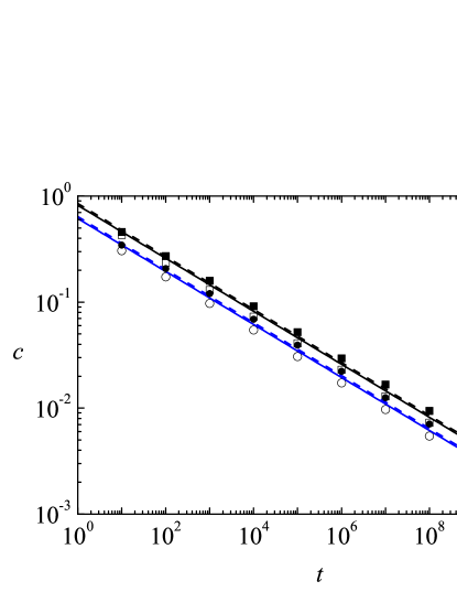
Figure 1: Reactant concentration vs time on a lattice of $10^{4}$ sites with periodic boundary conditions. $c(0)=1$, $\alpha=0.5$. Symbols give results of numerical simulations with kill (open symbols) and no-kill (black symbols) protocols. Circles: Mittag-Leffler-based waiting time distribution. Squares: Pareto waiting time distribution. Solid lines: our theory, Eq. (40), with $K_{alpha,P}$ (upper line) and with $K_{\alpha,ML}$ (lower line). Broken lines: approximations $c(t)\sim 1/S_{P}(t)$ (upper) and $c(t)\sim 1/S_{ML}(t)$ (lower). For a definition of symbols and for quantitative fits to the various lines see text. In addition, in all the figures of this paper the error bars are smaller than the symbol sizes.

of surviving $A$ particles as a function of time for $\alpha=0.5$ and an initial concentration $c(0)=1$. The initial concentration is sufficiently high for there to be essentially no transient behavior before the asymptotic power law dependence of $c(t)$ takes over, as evidenced by the straight lines. First, note the comparison between the simulation (sim) results with a Pareto-like waiting time distribution (squares) and those of a Mittag-Leffler form (circles). Both are essentially linear, as expected. The slopes are the same, but the Pareto results are a little higher. A best fit leads to $c_{P,sim}\sim 0.751~{}t^{-0.252}$ and $c_{M,sim}\sim 0.541~{}t^{-0.250}$. The open symbols are “kill” simulations (and the fits just given are for this case), while the solid symbols are for “no-kill.” The “no-kill” rule leads to consistently higher concentrations. This makes sense since the survivor at each reaction event is the $A$ that arrived first at the reaction site, and it remains there longer (due to aging) than would the other reaction partner. This leads to its longer survival.

While these results and comparisons are interesting, our most important task is to compare these results with those of our theory, which is shown by the upper solid line for the Pareto case and the lower solid line for the Mittag-Leffler case. The slopes are in excellent agreement with those of the simulations. The coefficients fall precisely between the “kill” and “no-kill” results. Specifically, we find that $c_{P,theory}\sim 0.819~{}t^{-0.25}$ and $c_{ML,theory}\sim 0.615~{}t^{-0.25}$. One might be tempted to conjecture that the theoretical model in some sense lies between the “kill” and “no-kill” scenarios. For example, perhaps the model is most germane if “kill” or “no-kill” are randomly selected according to some appropriate distribution. For now, this remains a matter of conjecture.

Finally, one additional result is shown in Fig. 1, namely, the validity of the relation between the concentration of surviving reactant and the distinct number of sites visited by a random walker, $c(t)\sim 1/S(t)$ MetKlaPhysRep ; Yustebook . The dashed lines show $1/S(t)$, with the upper dashed line corresponding to the Pareto case, $1/S_{P}(t)\sim 0.853~{}t^{-0.25}$, and the lower dashed line associated with the Mittag-Leffler choice, $1/S_{ML}(t)\sim 0.641~{}t^{-0.25}$.

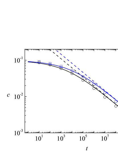
Figure 2: Reactant concentration vs time on a lattice of $10^{4}$ sites with periodic boundary conditions. $c(0)=0.1$, $\alpha=0.5$, showing transient behavior. Symbols give results of Numerical simulations with “kill” protocol for Pareto (squares) and Mittag-Leffler-based (circles) waiting time distribution. Solid lines: our theory, Eq. (40), with $K_{\alpha,P}$ (upper line) and $K_{\alpha,ML}$ (lower line). Broken lines: asymptotic approximation for $c(t)$ as given in Eq. (31) for both cases.

Figure 2 again shows the concentration of surviving reactant as a function of time for $\alpha=0.5$ on a lattice of $10^{4}$ sites, but now we explore whether our full theory, Eq. (40), in fact also captures the transient behavior. We explore this behavior by starting with a lower initial concentration, $c(0)=0.1$. Clearly, the theory again works extremely well for all times. Here the simulations are carried out in the “kill” scenario only, and we have presented both the Pareto (squares) and Mittag-Leffler (circles) results. The solid curves are the theoretical results for the Pareto (upper) and Mittag-Leffler (lower) cases. The dashed lines are the asymptotic results Eq. (31) for the two cases.

We stress that the asymptotic exponent of time as predicted by all theories (including our earlier theory that suffers from other difficulties) is correct and agrees with simulation results, which also agree with each other. The different theories and simulations (Pareto vs Mittag-Leffler, “kill” vs “no-kill,” our earlier theory vs our current theory, distinct number of sites visited predictions) lead to different (but not wildly different) prefactors. A more stringent test is provided by the interparticle distribution function, for which we now present a series of figures.

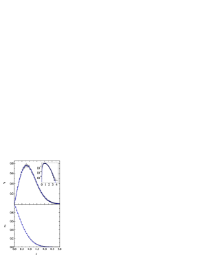
Figure 3: Asymptotic interparticle distribution function and empty interval function vs the scaled variable $z=c(t)x$ for the classic reaction-diffusion problem. The simulation results (symbols) are obtained with an exponential waiting time distribution on a lattice of 40,000 sites at time $t=6000$. The solid curves from the traditional exact theories are given in Eqs. (46) and (47). The upper panel shows the interparticle distribution function and the inset shows it on a logarithmic scale that exhibits the simulation scatter at extremely low densities. The lower panel shows the empty interval function.

In the (“normal”) reaction-diffusion problem the interparticle distribution function develops a growing gap at small distances. This gap arises as spatially close pairs react and are not replenished because diffusion is slow in one dimension. The gap explains the “anomalous” decay law $c(t)\sim t^{-1/2}$, called anomalous because it differs from the law of mass action behavior $c(t)\sim t^{-1}$ predicted for a Poissonian distribution of well-mixed reactants. Figure 3 shows these results as obtained from theory and simulations. They agree extremely well, which is a confirmation that we are in the asymptotic regime at time $t=6000$. The exact theoretical expressions are well known Torney ; Spouge ,

$$p(z)=\frac{\pi}{2}ze^{-\pi z^{2}/4}$$ (46)

and

$$E(z)={\rm erfc}(\sqrt{\pi}z/2).$$ (47)

This figure serves as a basis of comparison for subsequent subdiffusive results.

Figure 4 shows the same three panels for the subdiffusive case $\alpha=0.7$, but it is necessary to go to longer times, $t=10^{6}$, to arrive at the asymptotic behavior. The theoretical curves are obtained from Eqs. (33) and (III.3) and the simulations are carried out using a Pareto waiting time distribution with a “kill” rule. The agreement between theory and simulations is still excellent, with very small differences apparent near the maximum of the interparticle distance distribution. We have ascertained that we are in the asymptotic regime, so these differences are an indication of the approximate nature of the theory rather than of uncertainties pre-asymptotic transient effects.

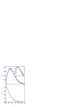
Figure 4: Asymptotic interparticle distribution function and empty interval function as a function of the scaled variable $z=c(t)x$ for $\alpha=0.7$. The simulation results (symbols) are obtained with a Pareto waiting time distribution and a “kill” rule on a lattice of 40,000 sites at time $t=10^{6}$. The solid theoretical curves are obtained from Eqs. (33) and (III.3). The upper panel shows the interparticle distribution function and the inset shows it on a logarithmic scale that exhibits the simulation scatter at extremely low densities. The lower panel shows the empty interval function.

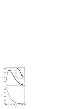
Figure 5: Asymptotic interparticle distribution function and empty interval function as a function of the scaled variable $z=c(t)x$ for $\alpha=0.2$. The simulation results (symbols) are obtained with a Pareto waiting time distribution and a “kill” rule on a lattice of 40,000 sites at time $t=10^{19}$. The solid theoretical curves are obtained from Eqs. (33) and (III.3). The upper panel shows the interparticle distribution function and the inset shows it on a logarithmic scale that exhibits the simulation scatter at extremely low densities. The lower panel shows the empty interval function.

Figure 5 shows the three panels once again, now for the extremely subdiffusive case $\alpha=0.2$. The particles spend a great deal of time simply waiting between jumps, and so it is necessary to go to much longer times, here $t=10^{19}$, to reach asymptotic behavior. The differences between theory and simulation are still small but certainly more noticeable. It is of course not clear whether the differences arise from the fact that the distribution of particles is affected by the reaction, or from the assumption of linearity of the evolution operator of the empty interval function, or both. In any case, it does not seem an exaggeration to assert that the theory is very good. It is also clear that a gap in the interparticle distance distribution develops no matter how subdiffusive the system, contrary to our earlier thinking ourold .

Two further issues are addressed in the following figures. In most of our simulation results we have used the “kill” rule whereby the walker that arrives at an already occupied site eliminates the particle that was there, and we have stated that agreement with our theory is better with this rule than with the “no-kill” rule whereby the newcomer is eliminated. Figure 6 shows three panels where this is illustrated for $\alpha=0.2$, $0.5$, and $0.8$ (the rule choice does not matter when $\alpha=1$). We see that as $\alpha$ decreases the differences in the simulation results for these two cases increase, and that the theory is closer to the “kill” results. Note that in these figures instead of a final simulation time we report a final simulation concentration to take advantage of the fact that $z$ depends on time only through the concentration and hence we avoid additional uncertanities. These differences point to the approximation inherent in the hypothesis that the reaction does not alter the spatial distribution of reactants. It does, although not by very much, especially if $\alpha$ is not extremely small.

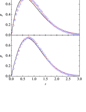
Figure 6: Interparticle distribution function $p(z)$. Symbols: simulation results with a Pareto waiting time distribution. Upside down triangles (red in color): “kill” rule. Right side up triangles (blue in color): “no-kill” rule. Lattice size $L=10000,c(0)=1,c(t_{final})=0.0025$. Upper panel: $\alpha=0.2$. Middle panel: $\alpha=0.5$. Lower panel: $\alpha=0.8$. The solid curves are calculated from Eq. (33).

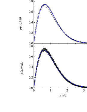
Figure 7: Interparticle distribution function for $\alpha=0.5$. Symbols: simulation results with a Mittag-Leffler waiting time distribution with $C(0)=0.1$. Upper panel: $t=10^{2}$. Middle panel: $t=10^{5}$. Lower panel: $t=10^{8}$. The solid curves are asymptotic, calculated from Eq. (33).

Finally, we briefly examine the approach of the interparticle distribution to its asymptotic behavior by plotting $p(x,t)/c(t)$ as a function of $xc(t)$, the scaling variable. Figure 7 shows the time progression of the distribution for $\alpha=0.5$ until its arrival at asymptotic behavior in the lower panel. It is preferable to use the Mittag-Leffler waiting time distribution for this progression as we have done in these simulations because of its advantages at early times compared to the Pareto distribution. The figure illustrates that the growth of the interparticle gap at early times is faster than at later times when it is determined by the scaling form, but that the system settles into its asymptotic form rather quickly.

VI Conclusions

We have presented a new theory for the coagulation reaction $A+A\to A$ on a lattice where the $A$’s perform a subdiffusive continuous time random walk characterized by the subdiffusive exponent $\alpha$. Our theory relies on the connection between continuous time random walks and fractional diffusion equations, and is based on two assumptions. The first hypothesis is that the evolution of the probability density for an empty interval of length $x$ at time $t$ in the presence of reactions is the same as the probability density that, in the absence of reactions, the distance between two subdiffusive particles that start at the same location at $t=0$ is $x$ at time $t$. The two probability densities are not equal because they obey different initial and boundary conditions. Only the evolution equations are assumed to be the same. The second hypothesis is that the (unknown) common equation of evolution for these two probability densities is linear. We have no analytic way of checking the validity of these assumptions, but the results of the theory are extremely close to those of numerical simulations in all cases tested. Some of the small differences are more likely ascribed to the second hypothesis, the assumption of linearity of the evolution operator, than the first, as explained in the earlier analysis.

We explicitly calculated the global reactant concentrations as a function of time. This is not a very discriminating measure of the quality of different theories; all the theories and implementations tested in this work lead to the same correct decay exponent of time, $c(t)\sim t^{-\alpha/2}$, and only the prefactors vary, albeit not dramatically. The well known association of $c(t)$ with the inverse of the distinct number of sites visited by a subdiffusive walker also gives the correct exponent and a prefactor within the range of our theory and simulation results. We also tested the early time transient behavior of $c(t)$ predicted by our theory and find that agreement with simulation results is also excellent.

A more stringent test of the theory is the interparticle distribution function, that is, the more “local” function $p(x,t)$. Again, we find our comparisons to show that the theory captures the simulation results very well, even for extremely subdiffusive systems. Most of the results that we present are asymptotic, but we also tested the validity of our theory in the transient regime, and found again that it works equally well.

An issue that we discussed at some length concerns a choice that must be made at the microscopic (continuous time random walk) level used in the simulations but not at level of the mesoscopic fractional diffusion equation used in the theory. The choice concerns the particle that vanishes when two $A$ particles land at the same location, the one that was there already or the one that just arrived. The results of simulations show the differences to be small but discernible in one dimension, which is evidence of aging Barkai ; we find that the agreement with our theory is slightly better with the first choice and perhaps would be even better with a combination of choices that allows for both possibilities with some probability distribution. We also discussed the choice of the waiting time distribution, an issue that becomes particularly important at early times and when $\alpha$ approaches unity.

Finally, we point to our work in higher dimensions ourlatest . In that work we considered the same reaction as well as the annihilation reaction but on a lattice with traps of random depths. The depths of the traps are associated with mean sojourn times that are finite and distributed according to a power law. Using a mean field formulation, we approximated this system by one that has identical fat-tailed waiting time distributions for each site, and show that in dimension $d=3$ the mean field model already captures the reaction dynamics and distribution functions of the original random trap system. In the mean field model, the “kill” and “no-kill” scenarios give the same results. A particularly important result in that work is that the waiting time distribution is unaffected by the reaction. In our one-dimensional model we start with the translationally invariant system, but also postulate, and show to lead to excellent results, an equivalence between evolution operators in the systems with and without reactions. We also point to the fact that the distribution develops a growing gap between particles ourold . The growth of the interparticle gap at early times is faster than at later times when it is determined by a scaling form, but in any case there is a gap. This “anomalous” distribution leads to the “anomalous” decay kinetics of the concentrarion, as in the case of normal diffusion in one dimension.

The analysis presented here can be adapted to the $A+A\to 0$ reaction, but the quantities to be calculated there are different because gap lengths don’t change continuously. One concentrates instead on the parity of the number of particles in a given interval Something2 ; Something3 , from which the desired quantities can in turn be derived. This will be a subject for future work.

- (1) E. Kotomin and V. Kazovkov, Modern Aspects of Diffusion-Controlled Reactions: Cooperative phenomena in Biomolecular Processes (Elsevier, Amsterdam, 1996).
- (2) J-C. Lin, C. R. Doering, and D. ben-Avraham, Chem. Phys. 146, 355 (1990); J-C. Lin, Phys Rev. A 44, 6706 (1991).
- (3) S. Habib, K. Lindenberg, G. Lythe, and C. Molina-París, J. Chem. Phys. 115, 73 (2001).
- (4) T. O. Masser and D. Ben-Avraham, Phys. Rev. E 066108 (2001).
- (5) S. B. Yuste and K. Lindenberg, Phys. Rev. Lett. 87, 118301 (2001); Chem. Phys. 284, 169 (2002).
- (6) I. M. Sokolov, S. B. Yuste, J. J. Ruiz-Lorenzo, and K. Lindenberg, Phys. Rev. E 79, 051113 (2009).
- (7) R. Metzler and J. Klafter, Phys. Rep. 339, 1 (2000).
- (8) B. H. Hughes, Random Walks and Random Environments, Volume 1: Random Walks, Clarendon Press, Oxford, 1995.
- (9) E. Scalas, R. Gorenflo, and F. Mainardi, Phys. Rev. E 69, 011107 (2004).
- (10) E. Barkai and Y-C. Cheng, J. Chem. Phys. 118, 6167 (2003).
- (11) M. Maseguerra and A. Zoia, Annals of Nuclear Energy 33, 223 (2006); ibid, Physica A 387, 2668 (2008).
- (12) D. C. Torney and H. McConnell, J. Phys. Chem.87, 1941 (1983).
- (13) J. L. Spouge, Phys. Rev. Lett.60, 871 (1988).
- (14) E Heinsalu, M Patriarca1, I Goychuk, and P Hänggi, J. Phys. Condens. Matter 19, 065114 (2007).
- (15) A. Blumen, J. Klafter, and G. Zumofen, “Models for reaction dynamics in glasses,” in Optical Spectroscopy of Glasses, edited by I. Zschokke, (Reidel, Dordrecht, 1986).
- (16) S. B. Yuste, K. Lindenberg, and J. J. Ruiz-Lorenzo, in Anomalous Transport: Foundations and Applications, edited by R. Klages, G. Radons, and I. M. Sokolov (Wiley-VCH, Berlin, 2008).