Observational Window Functions in Planet Transit Surveys

Abstract

The probability that an existing planetary transit is detectable in one’s data is sensitively dependent upon the window function of the observations. We quantitatively characterize and provide visualizations of the dependence of this probability as a function of orbital period upon several observing strategy and astrophysical parameters, such as length of observing run, observing cadence, length of night, transit duration and depth, and the minimum number of sampled transits. The ability to detect a transit is directly related to the intrinsic noise of the observations. In our simulations of observational window functions, we explicitly address non-correlated (gaussian or white) noise and correlated (red) noise and discuss how these two noise components affect transit detectability in fundamentally different manners, especially for long periods and/or small transit depths. We furthermore discuss the consequence of competing effects on transit detectability, elaborate on measures of observing strategies, and examine the projected efficiency of different transit survey scenarios with respect to certain regions of parameter space.

1. Introduction

The signal-to-noise ratio (SNR) of a planetary transit detection in photometric time series data can, in the simplest case, be approximated by:

$$SNR_{transit}=\frac{depth}{\sigma}\sqrt{n}.$$ (1)

In this equation, $depth$ is the transit depth in magnitudes, $\sigma$ represents the photometric measurement uncertainty in magnitudes per data point (assumed here to be the same for all data points), and $n$ equals the total number of data points observed during transit (Pont, 2006). One essential assumption in this equation is the absence of any statistically correlated (red) noise, i.e., only random (white) noise is present. White noise is defined as noise that is uncorrelated from data point to data point; typical sources are photon noise and sky background noise. The relative contribution of white noise to the total noise decreases with increasing brightness of the observed target and number of data points.

Pont (2006) and Pont et al. (2006) showed that calculations of transit SNRs with only white noise, as in Equation 1, is often insufficient and overly optimistic. Instead, one needs to account for the presence of red noise in calculations of SNRs and the corresponding yield projections for transit surveys. Red noise is defined as noise that is correlated from data point to data point; it is not necessarily removed through standard differential or ensemble photometry techniques. Typical sources of red noise may be weather, seeing changes, tracking/guiding errors, flatfielding errors, changes in airmass, or intrinsic astrophysical changes in target brightness. It does not change as a function of target magnitude, and is generally independent of the number of observational data points (see equation 9 in Pont et al., 2006). Thus, planetary transit searches are particularly sensitive to red noise, due to their focus on bright targets and high number of observational epochs: both are aimed to reduce white noise, and therefore make red noise the dominant component.

A detailed description of the transit detection SNR which includes both white and red noise components is given by Pont et al. (2006):

$$SNR_{transit} = \frac{depth}{\sqrt{\frac{1}{n^{2}}\sum_{i,j}cov[i;j]}}$$ (2)

$$= \frac{depth}{\sqrt{\frac{\sigma^{2}}{n}+\frac{1}{n^{2}}\sum_{i\neq j}cov[i;j]}},$$

where $cov[i;j]$ is the covariance matrix with elements $C_{ij}$ representing the correlation coefficents between the $i$-th and $j$-th measurements obtained during transit. All diagonal elements $C_{ii}=\sigma^{2}_{i}$ are not correlated with other measurements and thus represent the uncorrelated or white noise uncertainties in the $i$-th measurement. These diagonal elements are assumed to be the same, i.e., $\sigma_{i}=\sigma$ for all values of $i$.

In order to make the above equation more practically calculable, Pont et al. (2006) assume that statistical correlation among data points from different transits will be much weaker than among data points observed during the same transit. They furthermore separate the total noise into a purely uncorrelated (white) component $\sigma_{w}$ and a purely correlated (red) component $\sigma_{r}$ and derive an approximation of Equation 2:

$$SNR_{transit}=\sqrt{\frac{\left(depth\cdot n\right)^{2}}{\sum^{N_{tr}}_{k=1}\left[n^{2}_{k}\left(\frac{\sigma^{2}_{w}}{n_{k}}+\sigma^{2}_{r}\right)\right]}},$$ (3)

where $n$ is the total number of data points observed during all transits, $N_{tr}$ is the total number of transits observed, $n_{k}$ is the number of data points observed during the $k$-th transit, and $\sigma_{w}$ and $\sigma_{r}$ are the white and red noise components, respectively.

By means of Equations 1 and 3, it is clear that a planet transit SNR can be regarded as a function of transit survey strategy and astrophysical parameters (see §2). If this SNR exceeds a certain threshold value, then an existing transiting planet is, for the purposes of this paper, defined to be detectable in the data.

The window function determines the probability, as a function of planetary orbital period, that SNR_transit exceeds this threshold. In this paper, we examine the dependence of the detection probability upon several astrophysical and transit survey strategy parameters for a number of white noise and red noise assumptions as well as criteria based on a minimum number of transits sampled.

Since our calculations are based on existing transits, we note that the following aspects are not taken into account: the estimated frequency of transiting exoplanets, any non-circular orbits, multi planet systems, and detection of secondary transits. We also do not address the problem of false positives and how to weed them out. For more detailed studies of the above, we refer the reader to the following studies: frequency of (transiting) exoplanets: Gould et al. (2006) and Cumming et al. (2008); transit probability as a function of orbital elements: Barnes (2007), Burke (2008), and Kane & von Braun (2008); plus see Gaudi (2007) and Beatty & Gaudi (2008) and references therein for a comprehensive study of all factors influencing planet detections in transit surveys.

We briefly outline our methods in §2, which describes our algorithm in §2.1, along with a justification for the threshold SNR selection, and addresses the respective influences of varying white and red noise components (§2.2), as well as the consideration of sampling at least $N_{tr}$ transits with one’s data to constitute a detection (§2.3). We examine the effects of various survey strategy and astrophysical parameters in §3. Section 4 contains the application of window functions for selected scenarios and types of survey. We summarize and conclude in §5.

2. Algorithm and Parameters

In this Section, we provide a brief description of our algorithm and explain our choices of the globally used values of input parameters in our calculations in §3.

2.1. Description of the Algorithm

The window function algorithm used in this paper is based on counting data points observed during transit whose contribution to a virtual detection is dependent on the values of $\sigma_{w}$ and $\sigma_{r}$ as defined in Equations 2 and 3, typically measurable or calculable quantities in photometric time series surveys.

User-provided observing cadence, number of nights, and typical length of night are used to generate an observing time line. From the input stellar and planetary radii, we calculate transit depth and duration according to the equations in Seager & Mallén-Ornelas (2003) (except in §3.6 where we explicitly set transit depth and duration), thereby assuming a central transit (i.e., impact parameter $b=0$) and zero-length ingress and egress. For each orbital period, a family of light curves is generated for a range of starting phase angles; each with transits of user-defined photometric depths at the appropriate intervals.

In the simulations, the number of data points per transit ($n_{k}$), number of transits ($N_{tr}$) and total number of data points within all transits ($n$) are tracked. It should be noted that an observation has to fit fully within a transit to be counted toward $n$ and $n_{k}$ (that is, it needs to start after the beginning of the transit and terminate before the end of the transit), resulting in shorter exposure times’ being more favorable for transit detection in this algorithm. For every light curve, the SNR (Equations 1 and 3) is calculated. If, for a given phase angle, the SNR exceeds SNR_threshold, a transit is considered “detected”. The probability of detection (P_detection) for a given orbital period is simply the ratio of phase angles for which a transit was detected to the total number of phase angles.

Typical observational parameter values assumed in this paper (unless specifically noted) are: minutes for the observing cadence, one minute for the exposure time, tens of nights for observing run length, and few to ten hours for the typical time of observation spent during one night on the monitored target. Astrophysical parameter values are assumed to be around 1.0 and 0.1 solar radii for the parent star and orbiting planet, respectively, resulting in a transit depth of 0.01 mag. Transit duration depends on period, but typical duty cycles are in the 1% to few % range. Additionally, we set $\sigma_{w}$ and $\sigma_{r}$ to a few millimagnitudes (mmag). The threshold SNR is set to 7.0, based on the arguments in Jenkins et al. (2002) and specifically Pont et al. (2006, 2007), which each use thresholds of 7–9 as acceptable values for reducing false-alarms whilst maximizing real detections given a typical transit survey configuration.

We note that, in contrast to other some window function calculations in the astronomical literature, we only use the SNR criterion to quantify detections, along with an assumed minimum number of sampled transits, and we do not require that, e.g., a full transit be contained in the data (as in, e.g., Mallén-Ornelas et al., 2003; von Braun et al., 2005). We do not account for holes in the observing due to weather, telescope outages, or technical problems. Furthermore, as mentioned in §1, we only calculate the probability of detecting existiting primary transits in circular orbits. Finally, we assume that the number of out-of-transit data points sampled is much higher than the number of in-transit data points.

2.2. Red Noise and White Noise

As outlined in Pepper & Gaudi (2005); Pont et al. (2006); Aigrain & Pont (2007); von Braun & Ciardi (2008), red noise is the dominant source of noise in the regimes of brightness and number of observational epochs where transit surveys typically operate since red noise is independent of target brightness. We show this effect in §3.1. See Aigrain & Pont (2007) and Irwin et al. (2007) for an in-depth discussion of different noise properties and their calculations.

Typical ground-based survey estimates of $\sigma_{r}$, as defined in §1, are on the order of 2–6 millimagnitudes (mmag) (e.g., Pont et al., 2006; Irwin et al., 2007; Kane et al., 2008; Nutzman & Charbonneau, 2008). When subjected to detrending algorithms such as TFA (Kovács et al., 2005; Kovács & Bakos, 2007) or SYSREM (Tamuz et al., 2005), $\sigma_{r}$ can be reduced to 1–2 mmag.

It is worth pointing out that the influence of red noise is much less of a problem for targeted observations such as characterization of known planetary transits (see Gillon et al., 2008, for example).

Studies to date (e.g., Aigrain et al., 2008) have shown that the red noise in the space-based CoRoT mission (Baglin et al., 2006) is significantly lower than in ground-based counterparts, due in large part to the “removal of the atmosphere” (Pont et al., 2006; Beatty & Gaudi, 2008). Thus, the cause of any space based red noise not due to stellar variations is most likely caused by variations in the thermal environment of the spacecraft and detectors. Typical values for $\sigma_{r}$ in CoRoT light curves are on the order of 0.5 mmag (R. Alonso 2008, private communication; see also Aigrain et al., 2009).

2.3. Number of Sampled Transits

One criterion often used to calculate detection efficiency and related survey yield is the minimum number of sampled transits (i.e., the minimum number of transits during which any data were obtained). An important factor in the success of the widely used BLS algorithm (Kovács et al., 2002) is the initial folding of the data by a test period and subsequent search for transit-like features in the phased data. Thus, its power is really only realized for data that contain more than one sampled transit. We assume in this publication that the BLS algorithm has become an “industry standard” in the search for planetary transits, and we thus require the existence of at least two transits in the data for a transit detection, except for where we explicitly change this criterion (§3.5). It is worth noting that different simulations in the literature require different minimum numbers of transits sampled, such as three for Pont et al. (2006).

3. The Influence of Observational Window Functions and Astrophysical Parameters on Transit Detection Probability

Careful consideration of the various strategy aspects involved in planetary transit surveys and a number of astrophysical parameters will have significant effects on the detection efficiency of existing transits (Mallén-Ornelas et al., 2003; von Braun et al., 2005; Pepper & Gaudi, 2005; Beatty & Gaudi, 2008; von Braun & Ciardi, 2008; Beatty, 2009). This Section quantitatively illustrates these effects under consideration of the assumptions described in §2. For the sake of clarity, we vary one parameter at a time, leaving all others fixed to values justified in §1 and §2. In particular, §3.1 examines different values for red and white noise, §3.2 looks at various observing run lengths (with a given number of hours of observing per night), whereas §3.3 assumes a number of consecutive observing nights but varies their lengths. §3.4 investigates different observing cadences. In §3.5, we explicitly change the criterion of a minimum of two transits sampled for a detection that we mention in §2.3 to see how requiring a larger number decreases detection efficiency. §3.6 deals with different transit depths and durations.

The values of the parameters held constant in the respective calculation are given in the caption of the appropriate figure. The solid (blue) line shows the detection efficiency in the hypothetical case of zero red noise, and the dashed (red) line shows the same for a given $\sigma_{r}\neq 0$. The corresponding table shows the mean values of $P_{detection}$ for the ranges of orbital periods given in the first column under assumptions of the indicated magnitudes of $\sigma_{w}$ and $\sigma_{r}$.

3.1. Amount of Red Noise and White Noise

The contribution of red noise is independent of target brightness (unlike white noise, which is mostly due to photon noise for the brightest targets). Since planet transits are typically detected around the brightest sources in a given data set, red noise will be the dominant source of noise (Pepper & Gaudi, 2005; Pont et al., 2006; Aigrain & Pont, 2007; Beatty & Gaudi, 2008). Figures 1 and 2 along with Tables 1 and 2 quantitatively substantiate this statement, illustrating the influences of different amounts of red and white noises for different period ranges. As we mention in §2.2, typical values for the wide-field ground-based transit surveys before detrending are $\sigma_{w}\sim$ 5 mmag and $\sigma_{r}\sim$ 2–6 mmag, which reduces to $\sigma_{r}\sim$ 1–2 mmag after detrending.

The difference in $P_{detection}$ in Fig. 1 and Table 1 between $\sigma_{r}=1$ mmag and $\sigma_{r}=4$ mmag is very significant for longer periods. In addition, Fig. 2 and Table 2 show how small the influence of $\sigma_{w}$ upon $P_{detection}$ is for no or very little red noise. Thus, the value of minimizing the influences of red noise during observing (even at the expense of increasing $\sigma_{w}$ if necessary), and of applying detrending algorithms such as SYSREM (Tamuz et al., 2005) or TFA (Kovács et al., 2005; Kovács & Bakos, 2007) to one’s data as part of their reduction can hardly be overstated.

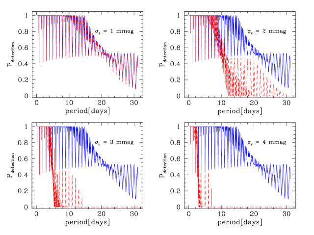
Figure 1.— Variable red noise and constant white noise ($\sigma_{w}=5$ mmag). The (blue) solid line indicates the detection efficiency for no red noise ($\sigma_{r}=0$) and is shown in all four panels. The (red) dashed line indicates detection efficiency for varying levels of $\sigma_{r}$ as indicated in the respective panel. Additional parameters are: SNR_threshold = 7.0, 60 consecutive observing nights with 8 hours of observing every night, an observing cadence of 5 minutes, $R_{star}=R_{\odot}$, $R_{planet}=0.1R_{\odot}$, $M_{star}=M_{\odot}$, $M_{planet}\ll M_{\odot}$. See Table 1 for mean values of $P_{detection}$ over various period ranges, and §3.1 for details.

Table 1Mean $P_{detection}$ Values for Different Magnitudes of $\sigma_{r}$

	$\sigma_{r}=0$	1 mmag	2 mmag	3 mmag	4 mmag
0–5 days	0.983	0.982	0.978	0.906	0.540
5–10 days	0.945	0.942	0.819	0.102	0.010
10–20 days	0.753	0.747	0.235	0.012	0.000
20–30 days	0.425	0.421	0.051	0.000	0.000

Note. — Mean values for $P_{detection}$ for various period ranges (column 1) as a function of different values of $\sigma_{r}$ (Fig. 1). Assumed parameters are given in the caption of Fig. 1. For discussion, see §3.1.

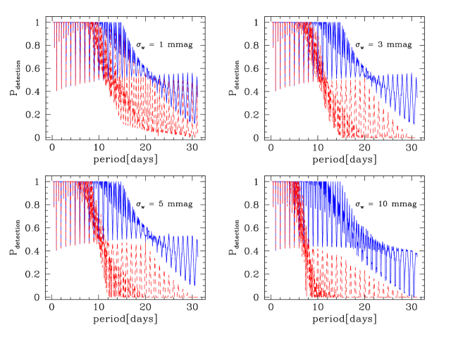
Figure 2.— Variable white noise and constant red noise. The value for $\sigma_{w}$ is given in the top right of every respective panel. The (blue) solid line indicates the detection efficiency $\sigma_{r}=0$, and the (red) dashed for $\sigma_{r}=2$ mmag. Additional parameters are: SNR_threshold = 7.0, 60 consecutive observing nights with 8 hours of observing every night, an observing cadence of 5 minutes, $R_{star}=R_{\odot}$, $R_{planet}=0.1R_{\odot}$, $M_{star}=M_{\odot}$, $M_{planet}\ll M_{\odot}$. See Table 2 for mean values of $P_{detection}$ over various period ranges, and §3.1 for discussion.

Table 2Mean $P_{detection}$ Values for Different Magnitudes of $\sigma_{w}$

$\sigma_{w}$	1 mmag	3 mmag	5 mmag	10 mmag
($\sigma_{r}=0$)
0–5 days	0.984	0.983	0.983	0.977
5–10 days	0.947	0.947	0.945	0.916
10–20 days	0.755	0.755	0.753	0.677
20–30 days	0.428	0.428	0.425	0.355
($\sigma_{r}=2$mmag)
0–5 days	0.981	0.980	0.978	0.967
5–10 days	0.897	0.857	0.819	0.444
10–20 days	0.412	0.281	0.235	0.072
20–30 days	0.131	0.058	0.051	0.017

Note. — Mean values for $P_{detection}$ for various period ranges (column 1) as function of $\sigma_{w}$ (Fig. 2). Assumed parameters are given in the caption of Fig. 2. For discussion, see §3.1.

3.2. Observing Run Length

For any kind of transit survey that has limited access to telescope time, the question of how long to spend on one field will occur at some point during the design of the observing strategy. At what point is it worth switching to a different field to increase the number of targets without overly reducing the probability of detecting existing transits in the data? We provide insight into the answer to this question in Fig. 3 and Table 3.

To first order, observing a field for few nights will yield an almost negligible probability of detection, potentially leading to a waste of telescope time. Alternatively, it may be wise not to stay on a single field for too long but rather to double the chances of detecting any planetary transits by switching fields and thus increasing the number of monitored stars. It is ultimately a question of the period range one is sampling in a given survey. As Fig. 3 shows for a typical set of parameters, “very hot Jupiters”, i.e., planets with periods up to $\sim$3 days per the definition in Gaudi et al. (2005), can be detected even with a residual presence of red noise and “only” 15 nights (eight hours per night) of monitoring. However, longer period planets ($\sim$6 days and longer) remain elusive (for $\sigma_{r}\geq$ 2mmag) until the length of the observing run exceeds 30 nights.

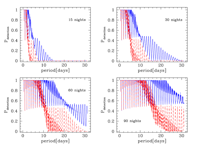
Figure 3.— The influence of length of observing run on the detection efficiency, shown for 15, 30, 60, and 90 nights (indicated in the respective panel). $\sigma_{w}$ is assumed to be 5 mmag. The (blue) solid line indicates the detection efficiency $\sigma_{r}=0$, and the (red) dashed for $\sigma_{r}=2$ mmag. Additional parameters are: SNR_threshold = 7.0, 8 hours of observing every night, an observing cadence of 5 minutes, $R_{star}=R_{\odot}$, $R_{planet}=0.1R_{\odot}$, $M_{star}=M_{\odot}$, $M_{planet}\ll M_{\odot}$. See Table 3 for mean values of $P_{detection}$ over various period ranges, and §3.2 for details.

Table 3Mean $P_{detection}$ Values for Different Observing Run Lengths

Nights	15	30	60	90
($\sigma_{r}=0$)
0–5 days	0.792	0.957	0.983	0.988
5–10 days	0.238	0.696	0.945	0.969
10–20 days	0.027	0.279	0.753	0.918
20–30 days	0.000	0.064	0.425	0.736
($\sigma_{r}=2$mmag)
0–5 days	0.482	0.865	0.978	0.987
5–10 days	0.020	0.189	0.819	0.954
10–20 days	0.000	0.022	0.235	0.618
20–30 days	0.000	0.000	0.051	0.188

Note. — Mean values for $P_{detection}$ for various period ranges (column 1) as function of observing run length (Fig. 3). Assumed parameters are given in the caption of Fig. 3. For discussion, see §3.2.

3.3. Length of Night

The amount of time for which a given target field can be observed from the ground during one night depends on its celestial coordinates, the location of the telescope, the time of year, and, of course, outages due to weather, or technical or other problems. Special cases are discussed below, such as space-based observing (§4.1) or synoptic surveys (§4.2).

The length of night can also depend on observing strategy. As an alternative to decreasing the number of nights spent on a single target field to increase the number of monitored stars (§3.2), one may instead choose to split the night up between two or more fields, thereby decreasing the number of hours spent on each one of them. We illustrate the effect of such strategies in Fig. 4 and Table 4 in which we assume basically the same parameters as for Figures 3 and 5 (see §3.4) for purposes of comparison. The situation shown in the bottom right panel can obviously only be achieved at numerically high latitudes on Earth during the respective winter season, or from space, but serves as a comparison to the scenarios encountered in transit surveys conducted from moderate latitudes. As in §3.2, the choice of strategy depends on the range of periods that is probed.

One expected and visible effect in Fig. 4 is the decreasing depth of spikes in $P_{detection}$ with longer lengths of night as the diurnal cycle becomes less of a factor in transit detection. As evidenced in Figures 7 and 10, the spikes eventually disappear altogether when observing becomes uninterrupted, as, e.g., from space.

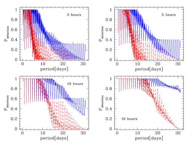
Figure 4.— The influence of the length of night on the detection efficiency, shown for 3, 5, 10, and 16 hours (indicated in the respective panel). $\sigma_{w}$ is assumed to be 5 mmag. The (blue) solid line indicates the detection efficiency $\sigma_{r}=0$, and the (red) dashed for $\sigma_{r}=2$ mmag. Additional parameters are: SNR_threshold = 7.0, a 5-minute observing cadence, 60 consecutive nights, $R_{star}=R_{\odot}$, $R_{planet}=0.1R_{\odot}$, $M_{star}=M_{\odot}$, $M_{planet}\ll M_{\odot}$. See Table 4 for mean values of $P_{detection}$ over various period ranges, and §3.3 for details.

Table 4Mean $P_{detection}$ Values for Different Night Lengths

Hours/Night	3	5	10	16
($\sigma_{r}=0$)
0–5 days	0.949	0.970	0.989	0.997
5–10 days	0.764	0.886	0.962	0.992
10–20 days	0.358	0.543	0.846	0.979
20–30 days	0.162	0.253	0.541	0.865
($\sigma_{r}=2$mmag)
0–5 days	0.839	0.954	0.986	0.996
5–10 days	0.182	0.462	0.912	0.985
10–20 days	0.049	0.092	0.402	0.801
20–30 days	0.017	0.028	0.075	0.237

Note. — Mean values for $P_{detection}$ for various period ranges (column 1) as function of length of night (Fig. 4). Assumed parameters are given in the caption of Fig. 4. For discussion, see §3.3.

3.4. Observing Cadence

Observing cadence is primarily dependent on telescope and detector characteristics as well as target brightness, with the goals that $\sigma_{w}$ is minimized, the target remains in the linearity regime of the detector, and the exposure time is not so long as to smear out phase information on any detectable planetary transit.

Similar to §3.2 and §3.3, however, the choice of cadence can also be used as a observing strategy parameter to increase the number of monitored stars at the expense of a lower sampling rate per field (by moving back and forth between fields between exposures, for instance). This effect is simulated in Fig. 5, and values for $P_{detection}$ for different period ranges are given in Table 5, which shows that the effect of changing from a cadence of one to several minutes does not greatly affect the calculated detection probability, especially for very small values of $\sigma_{r}$. It may therefore be worth considering changing between fields every one or few exposures to increase target number. The effects of red noise produced for such an observing strategy, however, such as flatfielding errors due to the fact that the stars may not be located in exactly the same position in the field as before, are dependent on aspects such as the pointing stability of the telescope used and would need to be explored for the respective observing setup.

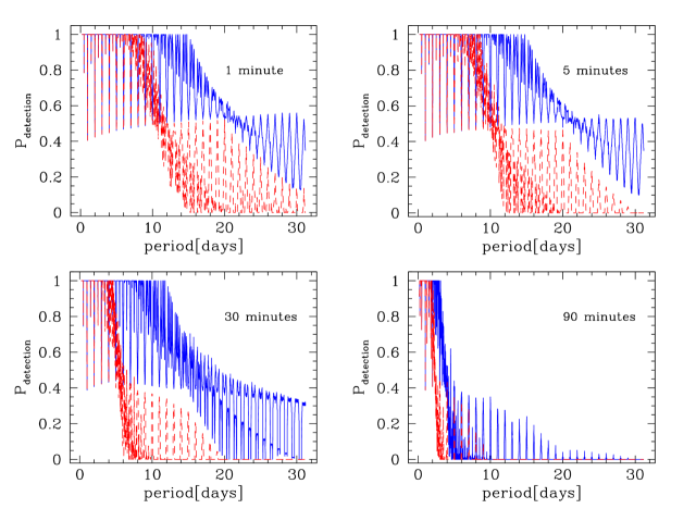
Figure 5.— The influence of observing cadence on the detection efficiency, shown for 1, 5, 60, and 90 minutes (indicated in the respective panel). $\sigma_{w}$ is assumed to be 5 mmag. The (blue) solid line indicates the detection efficiency $\sigma_{r}=0$, and the (red) dashed for $\sigma_{r}=2$ mmag. Additional parameters are: SNR_threshold = 7.0, 8 hours of observing every night, 60 consecutive nights, $R_{star}=R_{\odot}$, $R_{planet}=0.1R_{\odot}$, $M_{star}=M_{\odot}$, $M_{planet}\ll M_{\odot}$. See Table 5 for mean values of $P_{detection}$ over various period ranges, and §3.4 for details.

Table 5Mean $P_{detection}$ Values for Different Observing Cadences

Minutes	1	5	30	90
($\sigma_{r}=0$)
0–5 days	0.984	0.983	0.974	0.725
5–10 days	0.947	0.945	0.883	0.057
10–20 days	0.758	0.753	0.535	0.021
20–30 days	0.431	0.425	0.264	0.001
($\sigma_{r}=2$mmag)
0–5 days	0.980	0.978	0.936	0.457
5–10 days	0.864	0.819	0.214	0.015
10–20 days	0.293	0.235	0.037	0.000
20–30 days	0.071	0.051	0.000	0.000

Note. — Mean values for $P_{detection}$ for various period ranges (column 1) as function of observing cadence (Fig. 5). Assumed parameters are given in the caption of Fig. 5. For discussion, see §3.4.

3.5. Minimum Number of Sampled Transits

3.5.1 Two or more Transits

Transit duration is dependent on period (equation 3 in Seager & Mallén-Ornelas, 2003). Observational cadence determines the number of expected data points in a single transit. The combination of number of nights in the observing run and length of a given night sets the expected number of transits sampled during the monitoring campaign.

As explained in §2.3, we require a minimum of two transits sampled to constitute a detection. Note, however, that other predictions of survey yields in the literature use different numbers for different reasons, e.g., to be able to constrain period, which, with only two transits detected, would be subject to significant aliasing uncertainties, depending on the time elapsed between the two sampled transit events (see §7.4 in von Braun et al., 2005).

Fig. 6 and Table 6 show how the detection probability varies as a function of different minimum number of sampled transits. We note that, in this work, only one observation taken during a transit is enough to count this transit as sampled, but the detection is still a function of the transit SNR, as explained in §2, as well as the number of sampled transits.

It is interesting to observe that the detection probability of $\sigma_{r}=2$ mmag approaches the $\sigma_{r}=0$ case for higher minimum number of sampled transits, showing how the ”white noise only” case thus becomes increasingly equivalent to the realistic case with red noise present (Fig. 6 and Table 6 produce identical results for $\sigma_{r}=0$ and $\sigma_{r}=2$ mmag for more than five or more transits sampled). In the absence of knowledge of $\sigma_{r}$, requiring at least three or four detected transits in the data could therefore serve as a alternative for calculating a conservative estimate of survey yield.

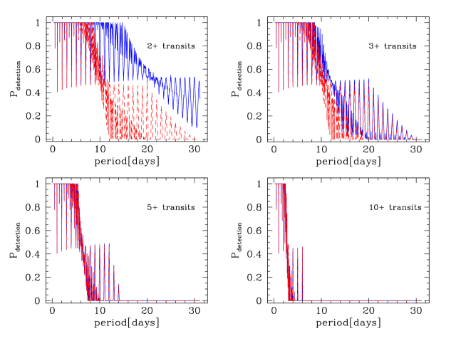
Figure 6.— The influence of the minimum number of transits sampled on the detection efficiency. Shown is the requirement that (at least) 2, 3, 5, and 10 transits (indicated in the respective panel) be sampled. $\sigma_{w}$ is assumed to be 5 mmag. The (blue) solid line indicates the detection efficiency $\sigma_{r}=0$, and the (red) dashed for $\sigma_{r}=2$ mmag. Additional parameters are: SNR_threshold = 7.0, a 5-minute observing cadence, 8 hours observing per night, 60 consecutive nights, $R_{star}=R_{\odot}$, $R_{planet}=0.1R_{\odot}$, $M_{star}=M_{\odot}$, $M_{planet}\ll M_{\odot}$. See Table 6 for mean values of $P_{detection}$ over various period ranges, and §3.5.1 for details.

Table 6Mean $P_{detection}$ Values for Different Minimum Number of Sampled Transits

Min. Number	2	3	5	10
($\sigma_{r}=0$)
0–5 days	0.983	0.981	0.965	0.549
5–10 days	0.945	0.878	0.313	0.008
10–20 days	0.753	0.339	0.023	0.000
20–30 days	0.425	0.066	0.000	0.000
($\sigma_{r}=2$mmag)
0–5 days	0.978	0.978	0.965	0.549
5–10 days	0.819	0.819	0.313	0.008
10–20 days	0.235	0.235	0.023	0.000
20–30 days	0.051	0.051	0.000	0.000

Note. — Mean values for $P_{detection}$ for various period ranges (column 1) as function of observing cadence (Fig. 6). Assumed parameters are given in the caption of Fig. 6. For discussion, see §3.5.1.

3.5.2 Detections Based on Single Transits

We now examine the case where it is deemed possible to detect a transit based on a minimum of one sampled transit. For this scenario, the detection probability may exhibit a non-intuitive behavior for very short and very long periods. To illustrate these points, we assume 5 “nights” of uninterrupted 24-hour (e.g., space-based or polar ground-based) observing (see Fig.7).

Short periods imply short transit durations. For a given cadence, there are few points per sampled transit. At the same time, short periods imply many transits sampled for a given observing run length. With increasing orbital period, the number of sampled transits decreases as the number of data points per transit increases, though not at the same rate. This effect can be seen for the short period range in Fig. 7, and it is most intuitively understood by considering the case for $\sigma_{r}=0$. Since $\sigma_{w}=$ transit depth = 10 mmag (Fig. 7), a detection simply requires $SNR_{threshold}^{2}=49$ data points observed during transit (Eq. 1), even if they are all located in a single transit. $P_{detection}$ goes to zero at a period of 2.5 days, which, for the stellar and planetary masses and radii given in the caption of Fig. 7, implies a transit length of around 161 minutes. For a 7-minute observing cadence, 23 data points can thus be collected during a single transit. For a 2.5 day period, one would expect to have two transits present in a 5-day observing run (24 hours of observing per “night”), but two transits would only contain 46 data points, and not the 49 required for $SNR_{transit}>SNR_{threshold}$. $P_{detection}$ in Fig. 7 therefore goes to zero at that point.

For periods longer than 3 days, however, the expected number of data points per transit is 24.5, and thus, sampling two transits somewhere in one’s data is sufficient for a detection, resulting in an increase of $P_{detection}$ with period as it approaches 3 days.

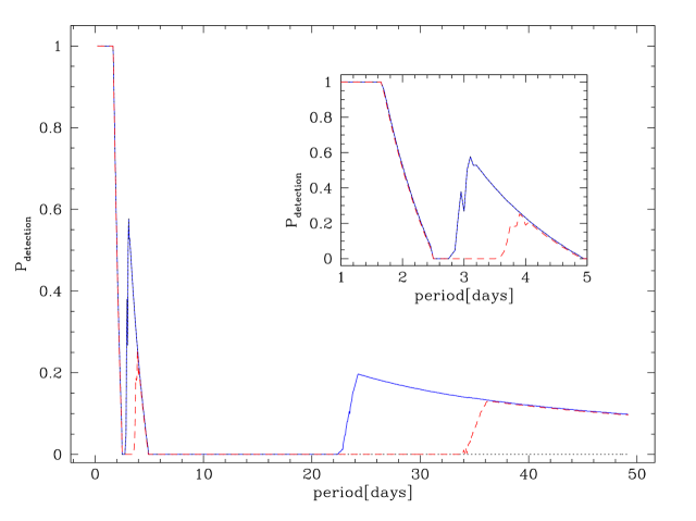
Figure 7.— The behavior of the detection probability as a function of period for a short, white-noise dominated monitoring campaign. $\sigma_{w}$ is assumed to be 10 mmag. $\sigma_{r}=0$ for the solid (blue) and dotted (black) lines; $\sigma_{r}=0.5$ mmag for the dashed (red) line. The solid (blue) and dashed (red) lines no longer assume a minimum number of sampled transits, whereas the dotted (black) line requires a minimum of two transits to be present in the data. Additional parameters are: SNR_threshold = 7.0, a 7-minute observing cadence, continuous observing (i.e., 24 hours observing per “night”), 5 consecutive nights, $R_{star}=R_{\odot}$, $R_{planet}=0.1R_{\odot}$, $M_{star}=M_{\odot}$, $M_{planet}=M_{Jupiter}$. The inset is a zoomed display of the behavior of $P_{detection}$ for periods between 1 and 5 days. See §3.5.2 for discussion.

An inverse effect can be observed at periods longer than the duration of the observing run and is again most easily explained by considering the $\sigma_{r}=0$ case. As expected, $P_{detection}$ drops to zero for periods longer than the observing run, since, although it is possible to sample one transit during the observing run, the length of this one transit is too short for enough data points (49) to be sampled during its duration (and it is obviously impossible to sample more than one transit, as indicated by the dotted line). This situation, however, changes as the period approaches 24 days (transit duration = 343 minutes). From that point on, the transit duration will be long enough to fit 49 data points at a 7-minute cadence. Therefore, if a single transit is observed, it is long enough to gather enough data to fulfill the threshold SNR criterion. Ultimately, the probability that any transit occurs at all during the observing run, and thus the detection efficiency, approaches zero.

3.6. Transit Depth and Duration

Throughout the paper, we calculate the transit depth and duration according to equations in Seager & Mallén-Ornelas (2003), thereby assuming a central transit, i.e., $i=90^{\circ}$ and $b=0$, as well as solar and Jupiter values for stellar and planetary radii and masses. In this subsection, we set those parameters to certain values that may not be consistent with physical laws, but are meant to illustrate the behavior of the detection probability as a function of transit duration and depth.

Transit depth is primarily a function of stellar and planetary radius, which we set to solar and Jupiter values before, resulting in a transit depth of 0.01 mag or 1% of the relative flux. In order to show how much more challenging the detection of smaller planets is, or conversely, how much easier the detection of larger planets is for given observing parameters, we vary transit depth in Fig. 8 and show mean $P_{detection}$ values in Table 7.

For a parent star with $R=R_{\odot}$, the panels represent planets of 0.3 $R_{Jupiter}$ (top left), 0.7 $R_{Jupiter}$ (top right), 1.0 $R_{Jupiter}$ (bottom left), and 1.4 $R_{Jupiter}$ (bottom right). Note that an Earth-sized planet would have a radius of around 0.1 $R_{Jupiter}$ and produce an eclipse around a solar-sized star with depth of 10% of that assumed in the top left panel, i.e., 0.0001 mag. It is worth pointing out how significant the difference in detection probability is for shallow transits between $\sigma_{r}=0$ and $\sigma_{r}\neq 0$, substantiating the claim that space-based observing is necessary to find very small planets (see also §4.1), as recently evidenced by the discovery of CoRoT-7b (Léger et al. in preparation; Rouan et al. in preparation; Bouchy et al. in preparation).

Transit duration is a function of orbital period, $i$, and stellar and planetary masses and radii. Rather than following the physical dependence on period, we set transit duration to fixed values of 1, 2, 5, and 10 hours in the four panels of Fig. 9 (see also Table 8), thereby still assuming values for the parameters mentioned in the figure caption, including a transit depth of 0.01 mag. While longer transits are obviously easier to detect, the increase of detectability with transit duration is slow but sensitively dependent on $\sigma_{r}$.

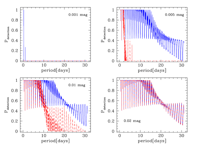
Figure 8.— The influence of the depth of transit on the detection efficiency, shown for 1, 5, 10, and 20 mmag (indicated in the respective panel). $\sigma_{w}$ is assumed to be 5 mmag. The (blue) solid line indicates the detection efficiency $\sigma_{r}=0$, and the (red) dashed for $\sigma_{r}=2$ mmag. Additional parameters are: SNR_threshold = 7.0, a 5-minute observing cadence, 8 hours observing per night, 60 consecutive nights, transit duration calculated using solar radius and mass for the star and Jupiter values for planetary mass and radius. See Table 7 for mean values of $P_{detection}$ over various period ranges, and §3.6 for details.

Table 7Mean $P_{detection}$ Values for Different Transit Depths

Transit Depth	1 mmag	5 mmag	10 mmag	20 mmag
($\sigma_{r}=0$)
0–5 days	0.009	0.977	0.983	0.984
5–10 days	0.000	0.916	0.945	0.947
10–20 days	0.000	0.677	0.753	0.755
20–30 days	0.000	0.355	0.425	0.428
($\sigma_{r}=2$mmag)
0–5 days	0.000	0.435	0.978	0.983
5–10 days	0.000	0.005	0.819	0.947
10–20 days	0.000	0.000	0.235	0.755
20–30 days	0.000	0.000	0.051	0.428

Note. — Mean values for $P_{detection}$ for various period ranges (column 1) as function of transit depth (Fig. 8). Assumed parameters are given in the caption of Fig. 8. For discussion, see §3.6.

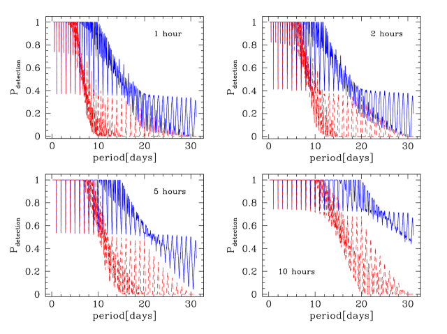
Figure 9.— The influence of transit duration on the detection efficiency, shown for 1, 2, 5, and 10 hours (indicated in the respective panel). $\sigma_{w}$ is assumed to be 5 mmag. The (blue) solid line indicates the detection efficiency $\sigma_{r}=0$, and the (red) dashed for $\sigma_{r}=2$ mmag. Additional parameters are: SNR_threshold = 7.0, a 5-minute observing cadence, 8 hours observing per night, 60 consecutive nights, transit depth = 0.01 mag. See Table 8 for mean values of $P_{detection}$ over various period ranges, and §3.6 for details.

Table 8Mean $P_{detection}$ Values for Different Transit Durations

Transit Duration	1 hour	2 hours	5 hours	10 hours
($\sigma_{r}=0$)
0–5 days	0.976	0.981	0.989	0.996
5–10 days	0.896	0.920	0.957	0.987
10–20 days	0.506	0.585	0.776	0.938
20–30 days	0.193	0.240	0.409	0.690
($\sigma_{r}=2$mmag)
0–5 days	0.964	0.975	0.986	0.995
5–10 days	0.414	0.676	0.879	0.974
10–20 days	0.058	0.126	0.272	0.609
20–30 days	0.010	0.028	0.050	0.121

Note. — Mean values for $P_{detection}$ for various period ranges (column 1) as function of transit duration (Fig. 9). Assumed parameters are given in the caption of Fig. 9. For discussion, see §3.6.

4. Application and Examples

The examples used in §3 to illustrate the influences of various observing strategy and astrophysical parameters on the transit detection probability resemble observing campaigns typical of the very successful wide-field transit surveys such as HAT, TrES, XO, SWASP, etc (e.g., Bakos et al., 2007; O’Donovan et al., 2006; McCullough et al., 2006; Pollacco et al., 2006). In contrast, this section shows examples and consequences of observational window functions for fundamentally different setups of monitoring projects.

4.1. Space Based Surveys

Compared to ground-based counterparts, space-based transit surveys such as CoRoT (Baglin et al., 2006) have the principal two advantages that (a) they are not subject to interruptions in observing due to the diurnal cycle (see §3.3), and that (b) they do not need to deal with the Earth’s atmosphere (see §3.1). The latter aspect in particular makes them the currently only realistic option of detecting Earth-sized planets around sun-like stars, which is one of the explicit goals of the recently launched Kepler Mission (Borucki et al., 2009).

Fig. 10 shows the detection probability for simulated space-based surveys of various lengths, loosely modeled after the long and short observing runs by the CoRoT satellite, thereby assuming somewhat generic parameters for survey strategy and photometric precision (see caption). The solid and dashed lines respectively indicate the detection probabilities for a Jupiter-sized planet and for the recently discovered exoplanet CoRoT-7b around its parent star, a K0 dwarf (transit depth $\sim$ 0.5 mmag; period $\sim$ 0.9 days). We note that our simulations of an Earth-sized planet around a solar-type star produce a detection probability of zero for all periods.

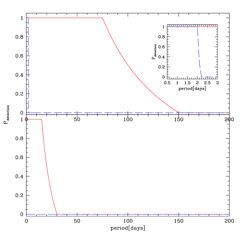
Figure 10.— Simulated space survey loosely based on the CoRoT short runs (bottom panel) and long runs (top panel). The solid (red) line indicates the detection probability of a Jupiter-sized planet around a solar-type star, the dashed (blue) line indicates the detection probability of the recently discovered exoplanet CoRoT-7b around its (K0 dwarf) parent star (transit depth $\sim$ 0.5 mmag; period $\sim$ 0.9 days). The inset in the top panel represents a zoomed display of the 0.5–3.0 day period range. Parameter values assumed in this simulation are: $SNR_{threshold}=7.0,\sigma_{w}=1$ mmag, $\sigma_{r}=0.5$ mmag, continuous observing with a 15-min cadence over 30 days (bottom panel) and 150 days (top panel). See §4.1 for details.

4.2. Synoptic Surveys

Synoptic surveys typically provide high-quality photometric time-series data of very low cadence but over extended periods of time. Thus, they are not primarily designed to find planetary transits but nevertheless present data sets that are worth probing for their existence (see for instance Plavchan et al., 2008). In fact, several transiting planets have been discovered a posteriori in the Hipparcos archives such as HD 209458b (Robichon & Arenou, 2000) and HD 189733b (Hébrard & Lecavelier Des Etangs, 2006).

The panels in Fig. 11 are produced by observational window functions of synoptic surveys loosely based on the (the future, ground-based) Large Synoptic Survey Telescope (LSST; Ivezic et al., 2008) in the top panel and (the space-based) Hipparcos mission (Perryman & ESA, 1997) in the bottom panel. For both panels, we require a $SNR_{threshold}=7.0$, at least two sampled transits, and assume solar and Jupiter values for stellar and planetary mass and radius. The principal differences between the two window functions in Fig. 11 are due to the different assumptions in $\sigma_{w}$ (5 mmag for top panel; 1.5 mmag for bottom panel) and $\sigma_{r}$ (1 mmag for top panel; 0.5 mmag for bottom panel), and the different number of data points obtained over different lengths of time.

For the top panel, we assumed a cadence of a single, 30-second exposure time image every three nights, accumulated over around eight years, such that the total number of images is 1,000. The mean value for $P_{detection}$ over various period ranges are as follows:

• 0–10 days: $<P_{detection}>$ = 0.555;

• 10–50 days: $<P_{detection}>$ = 0.239;

• 50-100 days: $<P_{detection}>$ = 0.025;

• 100–200 days: $<P_{detection}>$ = 0.007;

For the bottom panel, we chose a cadence based on the actual observations of a Hipparcos star with 190 epochs, downloaded from the NASA Star and Exoplanet Database. Basically, the 190 observations were obtained over three years in groups of several images every few tens of days. The mean value for $P_{detection}$ over various period ranges are as follows:

• 0–10 days: $<P_{detection}>$ = 0.746;

• 10–50 days: $<P_{detection}>$ = 0.156;

• 50-100 days: $<P_{detection}>$ = 0.034;

• 100–200 days: $<P_{detection}>$ = 0.012;

Finally, it should be noted that we ran the equivalent simulations to the ones in Fig. 11, but thereby assuming an Earth-sized planet instead of a Jupiter-sized one. Both detection probabilities were identical to zero for all periods.

Figure 11.— Simulated synoptic surveys loosely modeled after LSST (top panel) and Hipparcos (bottom panel). The insets are zoomed regions for the shorter periods. We assume solar-type stars and Jovian planets in these simulations. The 1,000 observations in the top panel are obtained over eight years, whereas the 190 observations in the bottom panel are taken over three years. See §4.2 for details.

5. Discussion and Conclusion

This work quantitatively illustrates the influence of a number of observing strategy and astrophysical parameters on the detection efficiency of existing planetary transits as a function of period under general assumptions listed in §2.1 and parameters given in the various figure captions. The influences of red and white noises upon this detection efficiency are first examined in their own right, and then included in every simulation of the aforementioned parameters. Red noise is confirmed to be the dominant challenge to overcome in the search for planetary transits, as seen in the discussion in §3.1, Figures 1 and 2, and Tables 1 and 2. All parameters being equal, a factor 4 increase in $\sigma_{r}$ produces a much more significant reduction in $P_{detection}$ than a factor 10 increase in $\sigma_{w}$.

In particular, we explicitly address controllable strategy parameters such as the number of nights for which one may choose to monitor a given target field, the number of hours per night one may stay on this field, and the observational cadence with which the field is monitored. We furthermore examine the influence of astrophysical parameters on detection efficiency, such as transit depth and duration. Finally, we look at parameters typically involved in the calculation of the projected yield of a given transit survey such as the minimum number of transits required for detections, and illustrate two non-intuitive effects that occur when the criterion of a minimum number of sampled transits is abandoned and detection is based only on SNR. Along with visualization of the effects caused by the various parameters in the figures, we provide quantitative means of comparison for different period ranges in the accompanying tables.

A consideration that did not factor into the calculation of $P_{detection}$ is the fraction of data points outside of transit (we assumed that this fraction is much higher than the number of points sampled in transit). In order to detect a transit in one’s data, one needs to have both brightness levels well measured such that the difference between them becomes signficant enough to enable a detection. For instance, an observing run that only obtains data during transit would, by the metrics used in this paper, detect the transit, provided the SNR is high enough. In real life, however, the data would appear perfectly flat and no sensible algorithm would flag the signal as a possible planetary transit. Obviously, sparse cadences are more susceptible to this admittedly pathologic pitfall than well sampled ones. One scenario where one may encounter a problem like this would be in the attempt to detect transits among long-period planets discovered by radial velocity work, which would tend to exhibit long transit durations.

More generally, we caution that the detection of an existing transit in “real life” is dependent on a large number of properties of the data reduction and analysis pipeline and transit detection methods, including human experience and human error potential, which cannot possibly be parametrized as an ensemble or included in any code. Therefore, the significance of our results and predictions, although quantitative, are necessarily subject to an unknown fudge or scaling factor. As pointed out by Beatty & Gaudi (2008), the non-uniformity of the definitions of detection criteria cause the largest uncertainty in transit survey yield predictions.

Nevertheless, we specifically allowed for parameters that are typically calculable in transit survey designs to be used as input to the code in order to make it as practically applicable as possible. Consequently, even in the presence of the unknown fudge factor mentioned above, comparisons between different observing strategies is quantitatively possible to optimize survey yield. For instance, under some circumstances it appears much more favorable to increase the observational cadence to add a second monitoring field to one’s project than switching fields in the middle of the night or in the middle of the observing run (see §§3.2, 3.3, and 3.4), provided it is possible to repeatedly achieve very good pointing of the telescope to reduce the additional red noise component that might arise from flatfielding errors otherwise. Thus, it may well be advisable for transit surveys to consider this trade-off between cadence and fields monitored as it can lead to a dramatic change in the predicted planet yield of the survey.

Furthermore, the examination of the effects of red and white noise in §3.1 and throughout the paper give quantitative insight into what size of planet one may expect to realistically detect in one’s data, given observing strategy parameters. In general, the depth of transit one may hope to detect in one’s data needs to be larger than the magnitude of $\sigma_{r}$, as seen in §3.6 and evidenced Figures 8 and 10. This is confirmed very well in Fig. 10, showing that the detection of CoRoT-7b around its parent star, given their sizes and orbital period, are right at the limits of the CoRoT satellite for a single long run (i.e., without combining data from several runs).

The code used for all calculations in this paper is available from KvB upon request.

References

- Aigrain et al. (2008) Aigrain, S., Collier Cameron, A., Ollivier, M., Pont, F., Jorda, L., Almenara, J. M., Alonso, R., Barge, P., Bordé, P., Bouchy, F., Deeg, H., de La Reza, R., Deleuil, M., Dvorak, R., Erikson, A., Fridlund, M., Gondoin, P., Gillon, M., Guillot, T., Hatzes, A., Lammer, H., Lanza, A. F., Léger, A., Llebaria, A., Magain, P., Mazeh, T., Moutou, C., Paetzold, M., Pinte, C., Queloz, D., Rauer, H., Rouan, D., Schneider, J., Wuchter, G., & Zucker, S. 2008, A&A, 488, L43
- Aigrain & Pont (2007) Aigrain, S. & Pont, F. 2007, MNRAS, 378, 741
- Aigrain et al. (2009) Aigrain, S., Pont, F., Fressin, F., Alapini, A., Alonso, R., Auvergne, M., Barbieri, M., Barge, P., Borde, P., Bouchy, F., Deeg, H., de la Reza, R., Deleuil, M., Dvorak, R., Erikson, A., Fridlund, M., Gondoin, P., Guterman, P., Jorda, L., Lammer, H., Leger, A., llebaria, A., Magain, P., Mazeh, T., Moutou, C., Ollivier, M., Paezold, M., Queloz, D., Rauer, H., Rouan, D., Schneider, J., Wuchterl, G., & Zucker, S. 2009, ArXiv e-prints
- Baglin et al. (2006) Baglin, A., Auvergne, M., Barge, P., Deleuil, M., Catala, C., Michel, E., Weiss, W., & The COROT Team. 2006, in ESA Special Publication, Vol. 1306, ESA Special Publication, ed. M. Fridlund, A. Baglin, J. Lochard, & L. Conroy, 33–+
- Bakos et al. (2007) Bakos, G. Á., Noyes, R. W., Kovács, G., Latham, D. W., Sasselov, D. D., Torres, G., Fischer, D. A., Stefanik, R. P., Sato, B., Johnson, J. A., Pál, A., Marcy, G. W., Butler, R. P., Esquerdo, G. A., Stanek, K. Z., Lázár, J., Papp, I., Sári, P., & Sipőcz, B. 2007, ApJ, 656, 552
- Barnes (2007) Barnes, J. W. 2007, PASP, 119, 986
- Beatty (2009) Beatty, T. G. 2009, in IAU Symposium, Vol. 253, IAU Symposium, 63–69
- Beatty & Gaudi (2008) Beatty, T. G. & Gaudi, B. S. 2008, ApJ, 686, 1302
- Borucki et al. (2009) Borucki, W., Koch, D., Batalha, N., Caldwell, D., Christensen-Dalsgaard, J., Cochran, W. D., Dunham, E., Gautier, T. N., Geary, J., Gilliland, R., Jenkins, J., Kjeldsen, H., Lissauer, J. J., & Rowe, J. 2009, in IAU Symposium, Vol. 253, IAU Symposium, 289–299
- Burke (2008) Burke, C. J. 2008, ApJ, 679, 1566
- Cumming et al. (2008) Cumming, A., Butler, R. P., Marcy, G. W., Vogt, S. S., Wright, J. T., & Fischer, D. A. 2008, PASP, 120, 531
- Gaudi et al. (2005) Gaudi, B. S., Seager, S., & Mallén-Ornelas, G. 2005, ApJ, 623, 472
- Gaudi (2007) Gaudi, S. 2007, in Astronomical Society of the Pacific Conference Series, Vol. 366, Transiting Extrasolar Planets Workshop, ed. C. Afonso, D. Weldrake, & T. Henning, 273–+
- Gillon et al. (2008) Gillon, M., Anderson, D. R., Demory, B. ., Wilson, D. M., Hellier, C., Queloz, D., & Waelkens, C. 2008, ArXiv e-prints
- Gould et al. (2006) Gould, A., Dorsher, S., Gaudi, B. S., & Udalski, A. 2006, Acta Astronomica, 56, 1
- Hébrard & Lecavelier Des Etangs (2006) Hébrard, G. & Lecavelier Des Etangs, A. 2006, A&A, 445, 341
- Irwin et al. (2007) Irwin, J., Irwin, M., Aigrain, S., Hodgkin, S., Hebb, L., & Moraux, E. 2007, MNRAS, 375, 1449
- Ivezic et al. (2008) Ivezic, Z., Tyson, J. A., Allsman, R., Andrew, J., Angel, R., & for the LSST Collaboration. 2008, ArXiv e-prints
- Jenkins et al. (2002) Jenkins, J. M., Caldwell, D. A., & Borucki, W. J. 2002, ApJ, 564, 495
- Kane et al. (2008) Kane, S. R., Clarkson, W. I., West, R. G., Wilson, D. M., Christian, D. J., Collier Cameron, A., Enoch, B., Lister, T. A., Street, R. A., Evans, A., Fitzsimmons, A., Haswell, C. A., Hellier, C., Hodgkin, S. T., Horne, K., Irwin, J., Keenan, F. P., Norton, A. J., Osborne, J., Parley, N. R., Pollacco, D. L., Ryans, R., Skillen, I., & Wheatley, P. J. 2008, MNRAS, 384, 1097
- Kane & von Braun (2008) Kane, S. R. & von Braun, K. 2008, ApJ, 689, 492
- Koen & Lombard (1993) Koen, C. & Lombard, F. 1993, MNRAS, 263, 287
- Konig & Timmer (1997) Konig, M. & Timmer, J. 1997, A&AS, 124, 589
- Kovács et al. (2005) Kovács, G., Bakos, G., & Noyes, R. W. 2005, MNRAS, 356, 557
- Kovács & Bakos (2007) Kovács, G. & Bakos, G. Á. 2007, in Astronomical Society of the Pacific Conference Series, Vol. 366, Transiting Extrasolar Planets Workshop, ed. C. Afonso, D. Weldrake, & T. Henning, 133–+
- Kovács et al. (2002) Kovács, G., Zucker, S., & Mazeh, T. 2002, A&A, 391, 369
- Lombard & Koen (1993) Lombard, F. & Koen, C. 1993, MNRAS, 263, 309
- Mallén-Ornelas et al. (2003) Mallén-Ornelas, G., Seager, S., Yee, H. K. C., Minniti, D., Gladders, M. D., Mallén-Fullerton, G. M., & Brown, T. M. 2003, ApJ, 582, 1123
- McCullough et al. (2006) McCullough, P. R., Stys, J. E., Valenti, J. A., Johns-Krull, C. M., Janes, K. A., Heasley, J. N., Bye, B. A., Dodd, C., Fleming, S. W., Pinnick, A., Bissinger, R., Gary, B. L., Howell, P. J., & Vanmunster, T. 2006, ApJ, 648, 1228
- Nutzman & Charbonneau (2008) Nutzman, P. & Charbonneau, D. 2008, PASP, 120, 317
- O’Donovan et al. (2006) O’Donovan, F. T., Charbonneau, D., Mandushev, G., Dunham, E. W., Latham, D. W., Torres, G., Sozzetti, A., Brown, T. M., Trauger, J. T., Belmonte, J. A., Rabus, M., Almenara, J. M., Alonso, R., Deeg, H. J., Esquerdo, G. A., Falco, E. E., Hillenbrand, L. A., Roussanova, A., Stefanik, R. P., & Winn, J. N. 2006, ApJ, 651, L61
- Pepper & Gaudi (2005) Pepper, J. & Gaudi, B. S. 2005, ApJ, 631, 581
- Perryman & ESA (1997) Perryman, M. A. C. & ESA, eds. 1997, ESA Special Publication, Vol. 1200, The HIPPARCOS and TYCHO catalogues. Astrometric and photometric star catalogues derived from the ESA HIPPARCOS Space Astrometry Mission
- Plavchan et al. (2008) Plavchan, P., Jura, M., Kirkpatrick, J. D., Cutri, R. M., & Gallagher, S. C. 2008, ApJS, 175, 191
- Pollacco et al. (2006) Pollacco, D. L., Skillen, I., Cameron, A. C., Christian, D. J., Hellier, C., Irwin, J., Lister, T. A., Street, R. A., West, R. G., Anderson, D., Clarkson, W. I., Deeg, H., Enoch, B., Evans, A., Fitzsimmons, A., Haswell, C. A., Hodgkin, S., Horne, K., Kane, S. R., Keenan, F. P., Maxted, P. F. L., Norton, A. J., Osborne, J., Parley, N. R., Ryans, R. S. I., Smalley, B., Wheatley, P. J., & Wilson, D. M. 2006, PASP, 118, 1407
- Pont (2006) Pont, F. 2006, in Tenth Anniversary of 51 Peg-b: Status of and prospects for hot Jupiter studies, ed. L. Arnold, F. Bouchy, & C. Moutou, 153–164
- Pont et al. (2007) Pont, F., Aigrain, S., Bakos, G., Brown, T., Collier Cameron, A., Deeg, H., Erikson, A., Guillot, T., Horne, K., Lecavalier, A., Moutou, C., Rauer, H., Queloz, D., & Seager, S. 2007, in Astronomical Society of the Pacific Conference Series, Vol. 366, Transiting Extrasolar Planets Workshop, ed. C. Afonso, D. Weldrake, & T. Henning, 3–+
- Pont et al. (2006) Pont, F., Zucker, S., & Queloz, D. 2006, MNRAS, 373, 231
- Robichon & Arenou (2000) Robichon, N. & Arenou, F. 2000, A&A, 355, 295
- Robinson (2005) Robinson, P. M. 2005, ArXiv Mathematics e-prints
- Seager & Mallén-Ornelas (2003) Seager, S. & Mallén-Ornelas, G. 2003, ApJ, 585, 1038
- Tamuz et al. (2005) Tamuz, O., Mazeh, T., & Zucker, S. 2005, MNRAS, 356, 1466
- Timmer (1998) Timmer, J. 1998, Phys. Rev. E, 58, 5153
- von Braun & Ciardi (2008) von Braun, K. & Ciardi, D. R. 2008, in IAU Symposium, Vol. 249, IAU Symposium, 93–100
- von Braun et al. (2005) von Braun, K., Lee, B. L., Seager, S., Yee, H. K. C., Mallén-Ornelas, G., & Gladders, M. D. 2005, PASP, 117, 141