Abstract

The onset of convection in the form of magneto-inertial waves in a rotating fluid sphere permeated by a constant axial electric current is studied through a perturbation analysis. Explicit expressions for the dependence of the Rayleigh number on the azimuthal wavenumber are derived in the limit of high thermal diffusivity. Results for the case of thermally infinitely conducting boundaries and for the case of nearly thermally insulating boundaries are obtained.

xx 1 1 This version: ; Received: date; Accepted: date; Published: date Onset of Inertial Magnetoconvection in Rotating Fluid Spheres Radostin D. Simitev^1,*, Friedrich H. Busse² Radostin Simitev and Friedrich Busse Correspondence: Radostin.Simitev@glasgow.ac.uk

1 Introduction

Buoyancy-driven motions of rotating, electrically conducting fluids in the presence of magnetic fields represent a fundamental aspect of the dynamics of stellar and planetary interiors, e.g. (Jones, 2011; Roberts and King, 2013; Charbonneau, 2014; Ogilvie, 2016). The problem of magnetic field generated and sustained by convection is rather difficult to attack both analytically and numerically because of its essential nonlinearity and scale separation (Glatzmaier, 2002; Miesch et al., 2015). Valuable insights can be gained by studying magnetoconvection, the simpler case of an imposed magnetic field, which has received much attention ever since the early work of Chandrasekhar (1961), see (Zhang and Schubert, 2000; Weiss and Proctor, 2014). For instance, propagation of rotating magnetoconvection modes excited in the deep convective region of the Earth’s core has been proposed as a possible mechanism for explaining features of observed longitudinal geomagnetic drifts (Hide, 1966; Malkus, 1967), see also the recent review of Finlay et al. (2010). A rather detailed classification of magnetoconvection waves in a rotating cylindrical annulus has been recently attempted by Hori et al. (2014) and Hori et al. (2015) who proceeded further to make useful comparisons with nonlinear spherical dynamo simulations and to provide estimates for the strength of the “hidden” azimuthal part of the magnetic field within the core. These authors used the rotating annulus model of Busse Busse (1970, 1986) and only considered values of the Prandtl number of the order unity. However, both spherical geometry as well as small values of the Prandtl number are essential features of a planetary or a stellar interior (Simitev and Busse, 2005). At sufficiently small values of the Prandtl number a different style of convection exists that is sometimes called inertial or equatorially-attached convection or thermo-inertial waves (Zhang and Busse, 1987; Ardes et al., 1997; Simitev and Busse, 2003; Plaut and Busse, 2005). In this limit convection oscillates so fast that the viscous force does not enter the leading-order balance. The latter is then reduced to the Poincaré equation in a rotating spherical system (Zhang, 1994, 1995; Zhang and Liao, 2017). On the longer time scale of the next order of approximation the buoyancy force maintains convection against the weak viscous dissipation. This regime of convection thus represents a transition between thermal convection and wave propagation in rapidly rotating geometries. It is important to understand how this regime of inertial convection is affected by an imposed magnetic field.

With this in mind, we study in the present paper the onset of magneto-inertial-convection. In particular, we consider a rotating fluid sphere permeated by a constant axial electric current as proposed by Malkus (1967) in the limit of low viscosity and high thermal diffusivity (small Prandtl number). A similarly configured problem was also investigated by Zhang and Busse (1995) who derived an explicit dependence of the critical Rayleigh number on the imposed field strength but were not able to obtain an explicit dependence on the azimuthal wavenumber of the modes since this requires the evaluation of a volume integral of the temperature perturbation. For this reason Zhang and Busse (1995) were unable to investigate the competition of modes and determine the actual critical parameters for the onset of convective motion. In an earlier paper we proposed a Green’s function method for the exact solution of the heat equation (Busse and Simitev, 2004) which then allowed the analytical evaluation of the integral quantities needed to find a fully explicit expressions for the critical Rayleigh number and frequency for the onset of convection and to study mode competition. Here we apply the same approach to the case of magneto-inertial convection and we consider both value and flux boundary conditions for the temperature.

In the following we start with the mathematical formulation of the problem in section 2. The special limit of a high ratio of thermal to magnetic diffusivity will be treated in section 3. The general case requires the symbolic evaluation of lengthy analytical expressions and will be presented in section 4. A discussion of the results and an outlook on related problems will be given in the final section 5 of the paper.

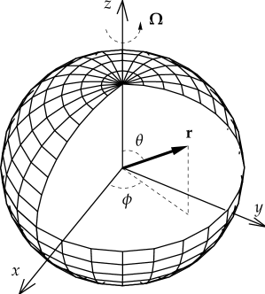
Figure 1: Geometrical configuration of the problem. A part of the outer spherical surface is removed to expose the interior of sphere to which the conducting fluid is confined.

2 Mathematical formulation of the problem

We consider a homogeneously heated and self-gravitating sphere as illustrated in figure 1. The sphere is filled with incompressible and electrically conducting fluid characterized by its magnetic diffusivity $\eta$, kinematic viscosity $\nu$, thermal diffusivity $\kappa$ and density $\varrho$. The sphere is rotating with a constant angular velocity $\Omega\mathbf{k}$ where $\mathbf{k}$ is the axial unit vector. The gravity field is given by $\mathbf{g}=-gr_{0}\mathbf{r}$ where $\mathbf{r}$ is the position vector with respect to the centre of the sphere, $r$ is its length measured in fractions of the radius $r_{0}$ of the sphere and $g$ is the amplitude of the gravitational acceleration. Following Malkus (1967), we assume that the fluid sphere is permeated by a toroidal magnetic field $\mathbf{B}\sim\mathbf{k}\times\mathbf{r}$. Since the Lorentz force like the centrifugal force can be balanced by the pressure gradient a static state of no motion exists with the temperature distribution $T_{S}=T_{0}-\beta r_{0}^{2}r^{2}/2$. We employ the Boussinesq approximation and assume constant material properties $\eta$, $\nu$, $\kappa$, and $\varrho$ everywhere except in the buoyancy term where the density is assumed to have a linear dependence on temperature with a coefficient of thermal expansion $\alpha\equiv(d\varrho/dT)/\varrho=$ const.

In order to study the onset of magnetoconvection in this system we consider the linearized momentum, magnetic induction, heat, continuity, and solenoidality equations,

$$\partial_{t}\tilde{\mathbf{u}}+\tau\mathbf{k}\times\tilde{\mathbf{u}}+\nabla(\pi-\tilde{\mathbf{b}}\cdot\mathbf{j}\times\mathbf{r})+(\mathbf{j}\times\mathbf{r})\cdot\nabla\tilde{\mathbf{b}}-\mathbf{j}\times\tilde{\mathbf{b}}=\tilde{\Theta}\mathbf{r}+P_{m}\nabla^{2}\tilde{\mathbf{u}},$$ (1a)

$$\partial_{t}\tilde{\mathbf{b}}-(\mathbf{j}\times\mathbf{r})\cdot\nabla\tilde{\mathbf{u}}+\mathbf{j}\times\tilde{\mathbf{u}}=\nabla^{2}\tilde{\mathbf{b}},$$ (1b)

$$\hat{R}\,\mathbf{r}\cdot\tilde{\mathbf{u}}+\nabla^{2}\tilde{\Theta}-(P/P_{m})\partial_{t}\tilde{\Theta}=0,$$ (1c)

$$\nabla\cdot\tilde{\mathbf{u}}=0,\quad\nabla\cdot\tilde{\mathbf{b}}=0,$$ (1d)

respectively, that govern the evolution of infinitesimal velocity perturbations $\tilde{\mathbf{u}}$, temperature perturbations $\tilde{\Theta}$, and magnetic field perturbations $\tilde{\mathbf{b}}$ away from the static state. The equations have been non-dimensionalised using the radius $r_{0}$ as a unit of length, $r_{0}^{2}/\eta$ as a unit of time, $\eta^{2}/g\alpha r_{0}^{4}$ as a unit of temperature and $\sqrt{\mu\varrho}\eta/r_{0}$ as a unit of magnetic flux density. The dimensionless magnetic field takes the form $\mathbf{j}\times\mathbf{r}+\tilde{\mathbf{b}}$, where $\mathbf{j}=j\mathbf{k}$ is the vector of the density of the imposed electric current. The problem is then characterised by five dimensionless parameters, namely the Rayleigh number, the Coriolis parameter, the Prandtl number, the magnetic Prandtl number $P_{m}$ and the non-dimensional current density given by

$$\hat{R}=\frac{\alpha g\beta r_{0}^{6}}{\eta\kappa},\enspace\tau=\frac{2\Omega r_{0}^{2}}{\eta},\enspace P=\frac{\nu}{\kappa},\enspace P_{m}=\frac{\nu}{\eta},\enspace j,$$ (2)

respectively. In fact, in the results obtained below the two Prandtl numbers enter only as their ratio $S=P/P_{m}=\eta/\kappa$. To signify that in our definition of the Rayleigh number the magnetic diffusivity replaces the kinematic viscosity we have attached a hat to $\hat{R}$.

3 Perturbation analysis

Without loss of generality we assume that the velocity, the magnetic field and the temperature perturbations have an exponential dependence on time $t$ and on the azimuthal angle $\phi$. Further, since both the velocity field and the magnetic field are solenoidal we use the poloidal-toroidal decomposition

$$\tilde{\mathbf{u}}=\mathbf{u}\exp\big{(}i(\omega\tau t+m\phi)\big{)}=\big{(}\nabla\times(\nabla v\times\mathbf{r})+\nabla w\times\mathbf{r}\big{)}\exp\big{(}i(\omega\tau t+m\phi)\big{)},$$ (3a)

$$\tilde{\mathbf{b}}=\mathbf{b}\exp\big{(}i(\omega\tau t+m\phi)\big{)}=\big{(}\nabla\times(\nabla h\times\mathbf{r})+\nabla g\times\mathbf{r}\big{)}\exp\big{(}i(\omega\tau t+m\phi)\big{)},$$ (3b)

$$\tilde{\Theta}=\Theta\exp\big{(}i(\omega\tau t+m\phi)\big{)}.$$ (3c)

Equation (1b) can now be written in the form

$$\mathbf{b}=\frac{m\gamma}{\omega}\mathbf{u}-\frac{i}{\omega\tau}\nabla^{2}\mathbf{b},$$ (4)

where the parameter $\gamma$ is defined as $\gamma=j/\tau$, and in the $\nabla$-operator the $\phi$-derivative is replaced by its eigenfactor $im$. This allows us to transform equation (1a) in the form,

$$i\omega\left(1-\frac{m^{2}}{\omega^{2}}\gamma^{2}\right)\mathbf{u} +\left(1-\frac{m}{\omega}\gamma^{2}\right)\mathbf{k}\times\mathbf{u}-\nabla\check{\pi}=\frac{1}{\tau}\Theta\mathbf{r}+\frac{P_{m}}{\tau}\nabla^{2}\mathbf{u}+\frac{m^{2}\gamma^{2}}{\omega^{2}\tau}\nabla^{2}\mathbf{u}$$

$$+\frac{2m\gamma^{2}}{i\omega^{2}\tau}\mathbf{k}\times\nabla^{2}\mathbf{u}+\frac{m\gamma}{\omega\tau}\nabla^{2}\mathbf{b}_{b}+\frac{2\gamma}{i\omega\tau}\mathbf{k}\times\nabla^{2}\mathbf{b}_{b}+\frac{P_{m}}{\tau}\nabla^{2}\mathbf{u}_{b},$$ (5)

where $\check{\pi}$ is the effective pressure. In equation (5) the magnetic field $\mathbf{b}$ appears only in the form of the boundary layer correction $\mathbf{b}_{b}$, required since the basic dissipationless solution does not satisfy all boundary conditions (Zhang and Busse, 1995). For the same reason the Ekman layer correction $\mathbf{u}_{b}$ must be introduced (Zhang, 1994).

Following the procedure of earlier papers (Zhang, 1994; Busse and Simitev, 2004) we use a perturbation approach and solve equation (1a) in the limit of large $\tau$, using the ansatz

$$\mathbf{u}=\mathbf{u}_{0}+\tau^{-1}\mathbf{u}_{1}+...,\quad\omega=\omega_{0}+\tau^{-1}\omega_{1}+...,\quad\mathbf{b}=\mathbf{b}_{0}+\tau^{-1}\mathbf{b}_{1}+...,$$ (6)

The heat equation is solved unperturbed.

3.1 Zeroth-order approximation

In the following we shall assume the limit of large $\tau$ such that in zeroth order of approximation the right hand side of equation (5) can be neglected. The left hand side together with the condition $\nabla\cdot\mathbf{u}=0$ is of the same form as the equation for inertial modes (Zhang, 1994; Busse and Simitev, 2004). In the nonmagnetic case the inertial modes corresponding to the sectorial spherical harmonics yield the lowest critical Rayleigh numbers for the onset of convection Busse and Simitev (2004). We shall assume that this property continues to hold as long as the parameter $\gamma$ is sufficiently small so that the nonmagnetic limit is approached in the left-hand side of equation (5). The sectorial inertial modes are given by

$$v_{0}=P_{m}^{m}(\cos\theta)f(r),\quad w_{0}=P_{m+1}^{m}(\cos\theta)\psi(r),$$ (7a)

with

$$f(r)=r^{m}-r^{m+2},\qquad\psi(r)=r^{m+1}\frac{2im(m+2)}{(2m+1)(\lambda_{0}(m^{2}+3m+2)-m)},$$ (7b)

where $$\lambda_{0}$$

$$\lambda_{0}=\frac{1}{m+2}\left(1\pm\sqrt{\frac{m^{2}+4m+3}{2m+3}}\right),$$ (7c)

is the frequency of the inertial modes. The sectorial magneto-inertial modes are then described by the same velocity field (7a) and by a magnetic field $\mathbf{b}_{0}=m\gamma\mathbf{u}_{0}/\omega_{0}$. In the above expressions the subscript $0$ refers to the dissipationless solution of equations (1). The frequency $\omega_{0}$ of the magneto-inertial waves is determined by

$$\lambda_{0}=\frac{\omega_{0}^{2}-m^{2}\gamma^{2}}{\omega_{0}-m\gamma^{2}},$$ (8)

which yields

$$\omega_{0}=\frac{\lambda_{0}}{2}\pm\sqrt{\frac{\lambda_{0}^{2}}{4}+m\gamma^{2}(m-\lambda_{0})}.$$ (9)

With account of (7c), this dispersion relation allows for a total of four different frequencies $\omega_{0}$. For small values of $\gamma^{2}$ these are given by

$$\omega_{01,2}=\frac{1}{m+2}\left(1\pm\sqrt{\frac{m^{2}+4m+3}{2m+3}}\right)+m^{2}\gamma^{2}(m+2)\left(1\pm\sqrt{\frac{m^{2}+4m+3}{2m+3}}\right)^{-1}-m\gamma^{2},$$ (10a)

$$\omega_{03,4}=-m^{2}\gamma^{2}(m+2)\left(1\pm\sqrt{\frac{m^{2}+4m+3}{2m+3}}\right)^{-1}+m\gamma^{2}.$$ (10b)

The upper sign in expression (10a) refers to retrogradely propagating modified inertial waves, while the lower sign corresponds to the progradely traveling variety. The effect of the magnetic field tends to increase the absolute value of the frequency in both cases. Expression (10b) describes the dispersion of the slow magnetic waves. The upper sign refers to the progradely traveling modified Alfven waves and the lower sign corresponds to retrogradely propagating modified Alfven waves.

3.2 First-order approximation

The magneto-inertial waves described by expressions (7a) satisfy the condition that the normal component of the velocity field vanishes at the boundary. This property implies that the normal component of the magnetic field vanishes there as well. Additional boundary conditions must be specified when the full dissipative problem described by (5) is considered. We shall assume a stress-free boundary with either a fixed temperature (case A) or a thermally insulating boundary (case B),

$$\mathbf{r}\cdot\mathbf{u}=\mathbf{r}\cdot\nabla(\mathbf{r}\times\mathbf{u})/r^{2}=0\enspace\mbox{ and }\enspace\left\{\begin{array}[]{ll}\Theta=0&\text{(case A)}\\ \partial_{r}\Theta=0&\text{(case B)}\end{array}\right\}\enspace\mbox{ at }\enspace r=1.$$ (11)

Additionally we shall assume an electrically insulating exterior of the sphere which requires

$$g=0\enspace\mbox{ at }\enspace r=1$$ (12)

and the matching of the poloidal magnetic field to a potential field outside the sphere.

After the ansatz (6) has been inserted into equation (5) such that terms with $\mathbf{u}_{1}$ appear on the left hand side, while those with $\mathbf{u}_{0}$ and $\omega_{0}$ appear on the right hand side, we obtain the solvability condition for the equation for $\mathbf{u}_{1}$ by multiplying it with $\mathbf{u}_{0}^{*}$ and averaging it over the fluid sphere,

$$i\omega_{1}\left\langle|\mathbf{u}_{0}|^{2}\right\rangle\Bigg{(}1+\left(\frac{m^{2}}{\omega_{0}^{2}}-\frac{m(\omega_{0}^{2}-m^{2}\gamma^{2})}{\omega_{0}^{2}(\omega_{0}-m\gamma^{2})}\right)\gamma^{2}\Bigg{)}$$ (13)

$$\hskip 28.45274pt=\langle\Theta\mathbf{r}\cdot\mathbf{u}_{0}^{*}\rangle+\left(\langle\mathbf{u}_{0}^{*}\cdot\nabla^{2}\mathbf{u}_{0}\rangle\frac{m\gamma}{\omega_{0}}+\langle\mathbf{u}_{0}^{*}\cdot\nabla^{2}\mathbf{b}_{0b}\rangle\right)\left(\frac{m}{\omega}-\frac{\omega_{0}^{2}-m^{2}\gamma^{2}}{\omega_{0}^{2}-m\omega_{0}\gamma^{2}}\right)\frac{\gamma}{\tau},$$

where the brackets $\langle...\rangle$ indicate the average over the fluid sphere and the $*$ indicates the complex conjugate. We have neglected all terms connected with viscous dissipation, i.e. we have assumed the vanishing of $P_{m}$, since we wish to focus on the effect of ohmic dissipation. The effects of viscous dissipation have been dealt with in the earlier paper (Busse and Simitev, 2004). Since $\langle\mathbf{u}_{0}^{*}\cdot\nabla^{2}\mathbf{u}_{0}\rangle$ vanishes, as demonstrated in (Zhang et al., 2001), we must consider only the influence of the boundary layer magnetic field $\mathbf{b}_{0b}$. It is determined by the equation

$$i\omega_{0}\tau\mathbf{b}_{0b}=\nabla^{2}\mathbf{b}_{0b}.$$ (14)

Since the solutions of this equation are characterized by gradients of the order $\sqrt{\tau}$, the boundary layer correction needed for the poloidal component is of the order $\sqrt{\tau}$ smaller than the correction needed for the toroidal component. For large $\tau$ we need to take into account only the contribution $g_{0b}$ given by

$$g_{0b} =-g_{0}(r=1)\exp\left(-(1+is)(1-r)\sqrt{|\omega_{0}|\tau/2}\right)$$

$$=-\frac{m\gamma}{\omega_{0}}w_{0}(r=1)\exp\left(-(1+is)(1-r)\sqrt{|\omega_{0}|\tau/2}\right),$$ (15)

where $s$ denotes the sign of $\omega_{0}$. The solvability condition thus becomes reduced to

$$i\omega_{1}\left\langle|\mathbf{u}_{0}|^{2}\right\rangle \Bigg{(}1+\left(\frac{m\gamma^{2}(m-\omega_{0})}{\omega_{0}(\omega_{0}-m\gamma^{2})}\right)\Bigg{)}$$ (16)

$$=\, \frac{1}{\tau}\langle\Theta\mathbf{r}\cdot\mathbf{u}_{0}^{*}\rangle-\frac{3}{2}\frac{m\gamma^{2}(m-\omega_{0})(s+i)}{(\omega_{0}-m\gamma^{2})\sqrt{2|\omega_{0}|\tau}}\int_{-1}^{1}|P_{m}^{m+1}|^{2}\mathrm{d}(\cos\theta)\$$

$$\times(m+1)(m+2)\left|\frac{2m(m+2)}{(2m+1)\left(\frac{\omega_{0}^{2}-m^{2}\gamma^{2}}{\omega_{0}-m\gamma^{2}}(m+1)(m+2)-m\right)}\right|^{2}.$$

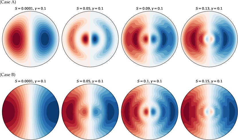
Figure 2: Contour plots of the (normalized) temperature perturbation $\Theta(r)$ of the preferred mode given by equations (17) and (26) in case A (top row) and case B (bottom row) with values of $S$ and $\gamma$ as specified in the panels and $\tau=10^{4}$, $m=1$ and frequency $\omega_{01}$. Expressions (17) and (18) for the limit $\tau S\ll 1$ appear identical to the plots in the first column.

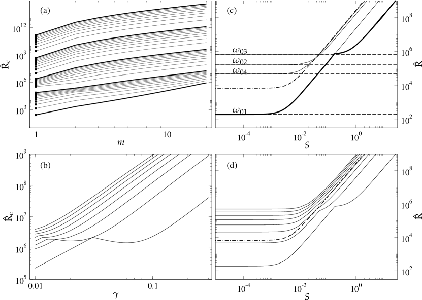
Figure 3: Case A. (a) The critical Rayleigh number $\mathrm{\hat{R}_{c}}$ as a function of the wave number $m$ for $\gamma=0.1$ and $\tau=10^{2}\dots 10^{6}$ increasing from bottom with log-scale decades given by the five thick lines. (b) The critical Rayleigh number $\mathrm{\hat{R}_{c}}$ as a function of $\gamma$ for $S=1$ and $m=1\dots 8$ increasing from bottom. (c) Competition of modes with increasing $S$ for $\gamma=0.1$ and $m=1$. Explicit expressions (20) in the limit $\tau S\ll 1$ are shown by broken lines. (d) The critical Rayleigh number $\mathrm{\hat{R}_{c}}$ as a function of $S$ for $\gamma=0.1$ and $m=1\dots 8$ increasing from bottom. The axisymmetric mode $m=0$ is given for comparison in panels (c,d) by a dot-dashed line. In panels (b) to (d) $\tau=10^{4}$.

3.2.1 Explicit expressions in the limit $\tau S\ll 1$

The equation (1c) for $\Theta$ can most easily be solved in the limit of vanishing $\omega_{0}\tau S$. In this limit we obtain for $\Theta$,

$$\Theta=P_{m}^{m}(\cos\theta)\exp(im\varphi+i\omega\tau t)q(r),$$ (17)

with

$$q(r)=\hat{R}\left(\frac{m(m+1)r^{m+4}}{(m+5)(m+4)-(m+1)m}-\frac{m(m+1)r^{m+2}}{(m+3)(m+2)-(m+1)m}-cr^{m}\right),$$ (18)

where the coefficient $c$ is given by

$$c=\begin{cases}\displaystyle\frac{m(m+1)}{(m+5)(m+4)-(m+1)m}-\displaystyle\frac{m(m+1)}{(m+3)(m+2)-(m+1)m},&\text{case A,}\\[10.0pt] \displaystyle\frac{(m+4)(m+1)}{(m+5)(m+4)-(m+1)m}-\displaystyle\frac{(m+2)(m+1)}{(m+3)(m+2)-(m+1)m},&\text{case B.}\end{cases}$$ (19)

Since $\Theta$ and the left hand side of equation (16) is imaginary, the real parts of the two terms on the right hand side must balance. We thus obtain for $\hat{R}$ the result

$$\hat{R}=s\sqrt{\frac{\tau}{2|\omega_{0}|}}\frac{\gamma^{2}(m-\omega_{0})}{(\omega_{0}-m\gamma^{2})}\left|\frac{m(m+2)}{\frac{\omega_{0}^{2}-m^{2}\gamma^{2}}{\omega_{0}-m\gamma^{2}}(m+1)(m+2)-m}\right|^{2}$$ (20)

$$\hskip 142.26378pt\times(2m+9)(2m+7)(2m+5)^{2}(2m+3)\frac{m+2}{m+1}\,\frac{1}{b},$$

where the coefficient $b$ assumes the values

$$b=\begin{cases}m(10m+27)&\text{case A,}\\[2.0pt] 14m^{2}+59m+63&\text{case B.}\end{cases}$$ (21)

Obviously the lowest value of $\hat{\mathrm{R}}$ is usually reached for $m=1$, but the fact that there are four different possible values of the frequency $\omega_{0}$ complicates the determination of the critical value $\mathrm{\hat{R}_{c}}$. Expression (20) is also of interest, however, in the case of spherical fluid shells when the ($m=1$)-mode is affected most strongly by the presence of the inner boundary. Convection modes corresponding to higher values of $m$ may then become preferred at onset since their $r$-dependence decays more rapidly with distance from the outer boundary according to relationships (7b).

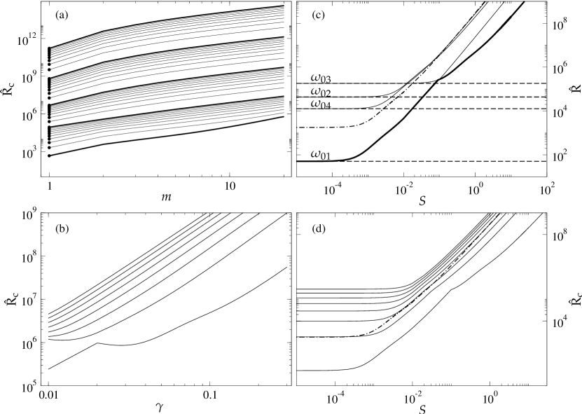
Figure 4: Same as figure 3 but in Case B.

Figure 5: The boundary where the transition from modes characterised by $\omega_{01}$ to modes characterised by $\omega_{03}$ occurs in various sections of the parameter space. The value of the parameters are $m=1$, $S=1$, $\gamma=0.1$, and $\tau=5000$ where they are not varied on the axes. Case A is denoted by a solid lines and Case B by broken lines.

3.2.2 Solution of the heat equation in the general case

For the solution of equation (1c) in the general case it is convenient to use the Green’s function method. The Green’s function $G(r,a)$ is obtained as solution of the equation

$$\left[\partial_{r}r^{2}\partial_{r}+\big{(}-i\omega_{0}\tau S\;r^{2}-m(m+1)\big{)}\right]G(r,a)=\delta(r-a),$$ (22)

which can be solved in terms of the spherical Bessel functions $j_{m}(\mu r)$ and $y_{m}(\mu r)$,

$$G(r,a)=\begin{cases}G_{1}(r,a)=A_{1}j_{m}(\mu r)\qquad&\text{for $0\leq r<a$},\\[2.0pt] G_{2}(r,a)=Aj_{m}(\mu r)+By_{m}(\mu r)\qquad&\text{for $a<r\leq 1$, }\end{cases}$$ (23)

where

$$\mu\equiv\sqrt{-i\omega_{0}\tau S},\quad A_{1}=\mu\left(y_{m}(\mu a)-j_{m}(\mu a)\frac{y_{m}(\mu)}{j_{m}(\mu)}\right),$$

$$A=-\mu j_{m}(\mu a)\frac{y_{m}(\mu)}{j_{m}(\mu)},\quad B=\mu j_{m}(\mu a).$$

A solution of equation (1c) can be obtained in the form

$$q(r)=-m(m+1)\hat{\mathrm{R}}\left(\int_{0}^{r}G_{2}(r,a)\left(a^{m}-a^{m+2}\right)a^{2}\mathrm{d}a+\int_{r}^{1}G_{1}(r,a)\left(a^{m}-a^{m+2}\right)a^{2}\mathrm{d}a\right).$$ (25)

Evaluations of these integrals for $m=1$ yield the expressions

$$q(r)=\begin{cases}\displaystyle\frac{2\hat{\mathrm{R}}}{(\omega_{0}\tau S)^{2}}\left(r(\mu^{2}+10)-\mu^{2}r^{3}-\displaystyle\frac{10\big{(}\mu r\cos(\mu r)-\sin(\mu r)\big{)}}{r^{2}\big{(}\mu\cos\mu-\sin\mu\big{)}}\right)&\text{case A,}\\[15.0pt] \displaystyle\frac{2\hat{\mathrm{R}}}{(\omega_{0}\tau S)^{2}}\left(r(2\mu^{2}+10)-\mu^{2}r^{3}-\displaystyle\frac{(\mu^{2}-10)\big{(}\mu r\cos(\mu r)-\sin(\mu r)\big{)}}{r^{2}\big{(}2\mu\cos\mu-(2-\mu^{2})\sin\mu\big{)}}\right)&\text{case B.}\end{cases}$$ (26)

Lengthier expressions are obtained for $m>1$. This first order approximation of the temperature perturbation is illustrated in Figure 2 for the preferred modes of inertial magnetoconvection. The preferred modes of convection at onset are determined by minimizing the values of the critical Rayleigh number $\hat{R}$ at given values of the other parameters. The critical Rayleigh number $\hat{R}$ and frequency $\omega_{1}$ are calculated on the basis of equation (16) using expressions (26). In the case $m=1$ we obtain

$$\hat{\mathrm{R}}={\frac{189}{20}}\, {\frac{s\sqrt{2\tau}{{\gamma}}^{2}\left(\omega_{0}-1\right)}{\sqrt{\left|\omega_{0}\right|}\left(\omega_{0}-{{\gamma}}^{2}\right)\left(6\,{\lambda_{0}}-1\right)^{2}}}$$ (27)

$$\times\begin{cases}\displaystyle\left(\mu^{-4}-525\mu^{-8}-175\;\text{Re}\left\{\frac{\sin\mu}{\mu^{6}(\mu\,\cos\mu-\sin\mu)}\right\}\right)^{-1}&\text{case A,}\\[10.0pt] \displaystyle\left(\mu^{-4}+231\mu^{-8}+7\;\text{Re}\left\{\frac{(\mu^{5}-8\mu^{3}+9\mu)\cos\mu-9\sin\mu}{\mu^{8}\big{(}(\mu^{2}-2)\sin\mu+2\mu\cos\mu\big{)}}\right\}\right)^{-1}&\text{case B,}\\ \end{cases}$$

where Re$\{\}$ indicates the real part of the term enclosed by $\{\}$. Expressions (27) have been plotted as functions of $S$ in figures 3(c) and 4(c) for the cases A and B, respectively. Four curves appear since there are four possible values of $\omega_{0}$ for each $m$. For values $S$ of the order $10^{-2}$ or less, expressions (20) are well approached. The retrograde mode corresponding to the positive sign in (7c) always yields the lower value of $\hat{R}$ but it looses its preference to the progradely traveling modified Alfven mode corresponding to the upper sign in (10b) as $S$ becomes of the order $10^{-1}$ or larger. This transition can be understood on the basis of the increasing difference in phase between $\Theta$ and $u_{r}$ with increasing $S$. While the mode with the largest absolute value of $\omega$ is preferred as long as $\Theta$ and $u_{r}$ are in phase, the mode with the minimum absolute value of $\omega$ becomes preferred as the phase difference increases since the latter is detrimental to the work done by the buoyancy force. The frequency perturbation $\omega_{1}$ usually makes only a small contribution to $\omega$ which tends to decrease the absolute value of $\omega$. This transition shifts towards smaller values of $S$ and $\gamma$ as $\tau$ is increased as illustrated in figure 5. The magneto-inertial convective modes corresponding to higher values of $m=1\dots 8$ exhibit similar behaviour as figures 3(d) and 4(d) demonstrate for the cases A and B, respectively. The value $m=1$ is always the preferred value of the wavenumber, except possibly in a very narrow range near $\gamma=0.03$ as indicated by figure 3(a,b) in the case A and possibly near $\gamma=0.02$ in the case B and figure 4(a,b). The axisymmetric mode $m=0$, given for comparison in panels (c) and (d) in figures 3 and 4, is never preferred in contrast to the purely non-magnetic case where it becomes the critical one near the transition from retrograde to prograde inertial convection modes as seen in figure 6.

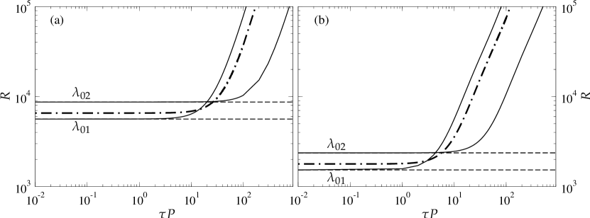
Figure 6: Competition of modes with increasing $\tau P$ in the non-magnetic case discussed in (Busse and Simitev, 2004). The Rayleigh number R as a function of $\tau P$ for $m=0$ (thick dash-dotted lines) and $m=1$ (thin lines). Results based on the explicit expressions (4.6) and (3.4) from (Busse and Simitev, 2004) are shown in solid lines and broken lines respectively in the case $m=1$. (a) Case A, fixed temperature boundary conditions. (b) Case B, insulating thermal boundary conditions.

For very large values of $\tau$ and $S$ the Rayleigh number $\hat{R}$ increases in proportion to $\sqrt{\tau}(\tau S)^{2}$ for fixed $m$. In spite of this strong increase $\Theta$ remains of the order $\tau^{3/2}S$ on the right hand side of equation (1a). The perturbation approach thus continues to be valid for $\tau\longrightarrow\infty$ as long as $S\ll 1$ can be assumed. For any fixed low value of $S$, however, the onset of convection in the form of prograde inertial modes will be replaced with increasing $\tau$ at some point by the onset in the form of columnar magneto-convection because the latter obeys an approximate asymptotic relationship for $R$ of the form $\tau^{4/3}$ (see, for example, Eltayeb et al. (1977)). This second transition depends on the value of $S$ and will occur at higher values of $\tau$ and $R$ for lower values of $S$. There is little chance that magneto-inertial convection occurs in the Earth’s core, for instance, since $S$ is of the order $30000$ while the usual estimate for $\tau$ is $10^{15}$ but it might be relevant for understanding of rapidly rotating stars with strong magnetic fields.

4 Discussion

A main result of the analysis of this paper is that for small values of the magnetic Prandtl number $P_{m}$ and $\gamma$ an azimuthal magnetic field exerts a stabilizing influence on the onset of convection in the form of sectorial magneto-inertial modes. As a consequence magneto-convection with azimuthal wave number $m=1$ is generally preferred at onset for both thermally-infinitely conducting and thermally-insulating boundaries. In contrast, in the absence of a magnetic field inertial modes with azimuthal wave number $m=1$ are preferred but only in the case of thermally-insulating boundaries, while in the case with infinitely conducting thermal boundaries large azimuthal wave numbers are preferred soon after moderately large rotation is reached Busse and Simitev (2004) and magnetic field is absent. Axisymmetric magneto-convection is never the preferred mode at onset while in the non-magnetic case it appears to be realized in a minute region of the parameter space only. These results are also in contrast to previous magnetoconvection results obtained for larger values of $P_{m}$ where a destabilizing role of the azimuthal magnetic field has been found.

The region of the parameter space investigated in the present paper differs considerably from those analysed in previous work. Most authors have emphasized regimes of high magnetic flux density where the magnetic field exerts a destabilizing influence and strongly decreases the critical Rayleigh number for onset of convection (see, for example, Eltayeb et al. (1977); Fearn (1979)). Unfortunately, no explicitly analytical results are possible in that region of the parameter space. Moreover the choice of parameter values has often been motivated by applications to the problem of the geodynamo in which case the parameter $S$ is large, perhaps as large as $10^{5}$, when molecular diffusivities are used. On the other hand, small values of $S$ may be relevant for magneto-convection in stars where a high thermal diffusivity is generated by radiation.

Conceptualization, F.H. and R.S; formal analysis, F.H. and R.S.; data curation, R.S.; writing–original draft preparation, F.B.; writing–review and editing, F.H. and R.S.; visualization, R.S. funding acquisition, R.S. The research of R.S. was funded by the Leverhulme Trust grant number RPG-2012-600. The authors declare no conflict of interest.

References

References

- Jones (2011) Jones, C.A. Planetary Magnetic Fields and Fluid Dynamos. Annual Review of Fluid Mechanics 2011, 43, 583–614. doi:\changeurlcolorblack10.1146/annurev-fluid-122109-160727.
- Roberts and King (2013) Roberts, P.H.; King, E.M. On the genesis of the Earth’s magnetism. Reports on Progress in Physics 2013, 76, 096801. doi:\changeurlcolorblack10.1088/0034-4885/76/9/096801.
- Charbonneau (2014) Charbonneau, P. Solar Dynamo Theory. Annual Review of Astronomy and Astrophysics 2014, 52, 251–290. doi:\changeurlcolorblack10.1146/annurev-astro-081913-040012.
- Ogilvie (2016) Ogilvie, G.I. Astrophysical fluid dynamics. Journal of Plasma Physics 2016, 82, 205820301. doi:\changeurlcolorblack10.1017/S0022377816000489.
- Glatzmaier (2002) Glatzmaier, G.A. Geodynamo Simulations—How Realistic Are They? Annual Review of Earth and Planetary Sciences 2002, 30, 237–257. doi:\changeurlcolorblack10.1146/annurev.earth.30.091201.140817.
- Miesch et al. (2015) Miesch, M.; Matthaeus, W.; Brandenburg, A.; Petrosyan, A.; Pouquet, A.; Cambon, C.; Jenko, F.; Uzdensky, D.; Stone, J.; Tobias, S.; Toomre, J.; Velli, M. Large-Eddy Simulations of Magnetohydrodynamic Turbulence in Heliophysics and Astrophysics. Space Science Reviews 2015, 194, 97–137. doi:\changeurlcolorblack10.1007/s11214-015-0190-7.
- Chandrasekhar (1961) Chandrasekhar, S. Hydrodynamic and hydromagnetic stability; International series of monographs on physics, Clarendon Press, 1961.
- Zhang and Schubert (2000) Zhang, K.; Schubert, G. Magnetohydrodynamics in Rapidly Rotating spherical Systems. Annual Review of Fluid Mechanics 2000, 32, 409–443. doi:\changeurlcolorblack10.1146/annurev.fluid.32.1.409.
- Weiss and Proctor (2014) Weiss, N.O.; Proctor, M.R.E. Magnetoconvection; Cambridge University Press, 2014. doi:\changeurlcolorblack10.1017/cbo9780511667459.
- Hide (1966) Hide, R. Free Hydromagnetic Oscillations of the Earth’s Core and the Theory of the Geomagnetic Secular Variation. Philosophical Transactions of the Royal Society A: Mathematical, Physical and Engineering Sciences 1966, 259, 615–647. doi:\changeurlcolorblack10.1098/rsta.1966.0026.
- Malkus (1967) Malkus, W.V.R. Hydromagnetic planetary waves. Journal of Fluid Mechanics 1967, 28, 793–802. doi:\changeurlcolorblack10.1017/S0022112067002447.
- Finlay et al. (2010) Finlay, C.C.; Dumberry, M.; Chulliat, A.; Pais, M.A. Short Timescale Core Dynamics: Theory and Observations. Space Science Reviews 2010, 155, 177–218. doi:\changeurlcolorblack10.1007/s11214-010-9691-6.
- Hori et al. (2014) Hori, K.; Takehiro, S.; Shimizu, H. Waves and linear stability of magnetoconvection in a rotating cylindrical annulus. Physics of the Earth and Planetary Interiors 2014, 236, 16 – 35. doi:\changeurlcolorblack10.1016/j.pepi.2014.07.010.
- Hori et al. (2015) Hori, K.; Jones, C.A.; Teed, R.J. Slow magnetic Rossby waves in the Earth’s core. Geophysical Research Letters 2015, 42, 6622–6629. doi:\changeurlcolorblack10.1002/2015GL064733.
- Busse (1970) Busse, F.H. Thermal instabilities in rapidly rotating systems. Journal of Fluid Mechanics 1970, 44, 441. doi:\changeurlcolorblack10.1017/s0022112070001921.
- Busse (1986) Busse, F.H. Asymptotic theory of convection in a rotating, cylindrical annulus. Journal of Fluid Mechanics 1986, 173, 545. doi:\changeurlcolorblack10.1017/s002211208600126x.
- Simitev and Busse (2005) Simitev, R.; Busse, F. Prandtl-number dependence of convection-driven dynamos in rotating spherical fluid shells. J. Fluid Mech. 2005, 532, 365. doi:\changeurlcolorblack10.1017/S0022112005004398.
- Zhang and Busse (1987) Zhang, K.K.; Busse, F.H. On the onset of convection in rotating spherical shells. Geophysical & Astrophysical Fluid Dynamics 1987, 39, 119–147. doi:\changeurlcolorblack10.1080/03091928708208809.
- Ardes et al. (1997) Ardes, M.; Busse, F.; Wicht, J. Thermal convection in rotating spherical shells. Physics of the Earth and Planetary Interiors 1997, 99, 55 – 67. doi:\changeurlcolorblack10.1016/S0031-9201(96)03200-1.
- Simitev and Busse (2003) Simitev, R.; Busse, F. Patterns of convection in rotating spherical shells. New J. Phys. 2003, 5, 97. doi:\changeurlcolorblack10.1088/1367-2630/5/1/397.
- Plaut and Busse (2005) Plaut, E.; Busse, F.H. Multicellular convection in rotating annuli. Journal of Fluid Mechanics 2005, 528, 119–133. doi:\changeurlcolorblack10.1017/s0022112004003180.
- Zhang (1994) Zhang, K. On coupling between the Poincaré equation and the heat equation. Journal of Fluid Mechanics 1994, 268, 211–229. doi:\changeurlcolorblack10.1017/S0022112094001321.
- Zhang (1995) Zhang, K. On coupling between the Poincaré equation and the heat equation: non-slip boundary condition. Journal of Fluid Mechanics 1995, 284, 239–256. doi:\changeurlcolorblack10.1017/S0022112095000346.
- Zhang and Liao (2017) Zhang, K.; Liao, X. Theory and Modeling of Rotating Fluids: Convection, Inertial Waves and Precession; Cambridge Monographs on Mechanics, Cambridge University Press, 2017. doi:\changeurlcolorblack10.1017/9781139024853.
- Zhang and Busse (1995) Zhang, K.; Busse, F.H. On hydromagnetic instabilities driven by the Hartmann boundary layer in a rapidly rotating sphere. Journal of Fluid Mechanics 1995, 304, 263–283. doi:\changeurlcolorblack10.1017/S0022112095004423.
- Busse and Simitev (2004) Busse, F.H.; Simitev, R. Inertial convection in rotating fluid spheres. Journal of Fluid Mechanics 2004, 498, 23–30. doi:\changeurlcolorblack10.1017/S0022112003006943.
- Zhang et al. (2001) Zhang, K.; Earnshaw, P.; Liao, X.; Busse, F.H. On inertial waves in a rotating fluid sphere. Journal of Fluid Mechanics 2001, 437, 103–119. doi:\changeurlcolorblack10.1017/S0022112001004049.
- Eltayeb et al. (1977) Eltayeb, I.A.; Kumar, S.; Hide, R. Hydromagnetic convective instability of a rotating, self-gravitating fluid sphere containing a uniform distribution of heat sources. Proceedings of the Royal Society of London A 1977, 353, 145–162. doi:\changeurlcolorblack10.1098/rspa.1977.0026.
- Fearn (1979) Fearn, D.R. Thermally driven hydromagnetic convection in a rapidly rotating sphere. Proceedings of the Royal Society of London. A 1979, 369, 227–242. doi:\changeurlcolorblack10.1098/rspa.1979.0161.