Can a student learn optimally from two different teachers?

Abstract

We explore the effects of over-specificity in learning algorithms by investigating the behavior of a student, suited to learn optimally from a teacher $\mathbf{B}$, learning from a teacher $\mathbf{B}^{\prime}\neq\mathbf{B}$. We only considered the supervised, on-line learning scenario with teachers selected from a particular family. We found that, in the general case, the application of the optimal algorithm to the wrong teacher produces a residual generalization error, even if the right teacher is harder. By imposing mild conditions to the learning algorithm form we obtained an approximation for the residual generalization error. Simulations carried in finite networks validate the estimate found.

I Introduction

Neural networks are connectivist models inspired on the dynamical behavior of the brain rumelhart . They are not only theoretically interesting models, they can also be used in a number of applications, from voice recognition systems to curve fitting software. Probably the properties that make neural networks most useful are their potentiality to store patterns and their capability for learning tasks.

One of the most well-studied types of networks is feed-forward. What characterizes a feed-forward network is that the flux of information follows a non-loopy path from input to output nodes, making the information processing much faster. Perceptrons papert are feed-forward networks with no internal nodes and only one output; they have been utilised for a number theoretical studies and applications of statistical mechanics techniques engel . In particular, the knowledge of Hebbian learning algorithms in an on-line scenario is quite complete.

In the present article we study the ability of a student J, using an algorithm for learning optimally from a specific teacher $\mathbf{B}$, to learn from a teacher $\mathbf{B}^{\prime}$. If a student is adapted to learn from a difficult teacher, it is not unreasonable to expect that it will be able to learn from an easier one. To formally analyze this problem we need to quantify the hardness of the teachers, set up the scenario where the learning process would take place and thus quantify the student’s performance.

Attempts to quantify hardness as an inherent property of the observed object have given origin to many formal definitions of complexity church ; turing0 ; hartmanis ; kolmogorov ; ming . Recently fra-0 L. Franco has proposed to quantify a (Boolean) function’s hardness by the size of the minimal set of examples needed to train a feed-forward network, with a predetermined architecture until reaching zero prediction error. He also found fra-1 ; fra-2 that in this minimal set there are many pairs of examples that, although only differing in a finite number $P=1,2,\dots$ of entries, they have different outputs, implying that these examples are located at each side of the classification boundary (similar to the support vectors for SVMs ton ). Further investigation showed that the average discrepancy of the function’s outputs (measure over neighboring pairs) is correlated to the generalization ability of the network implementing the function. In order to contour the use of the neural network and its minimal training set, Franco proposed to use the average distance sensitivity directly as a measure of the function’s hardness. This is probably the most suitable measure for our study given that the nature of the measure itself is linked to the concept of generalization ability.

The hardness measure we will use is the average output discrepancy taken over all pairs of inputs at a given Hamming distance P. Formally, for a given Boolean function $f:\left\{\pm 1\right\}^{N}\to\left\{\pm 1\right\},$ the $P$th distance sensitivity component $\mathfrak{d}_{P}^{N}[f]$ is the functional

$$\mathfrak{d}_{P}^{N}\left[f\right]=2^{-N}\sum_{\mathbf{S}\in\left\{\pm 1\right\}^{N}}{N\choose P}^{-1}\sum_{\mathbf{S}^{\prime}\in\upOmega_{P}\left(\mathbf{S}\right)}\frac{1-f\left(\mathbf{S}\right)f\left(\mathbf{S}^{\prime}\right)}{2}\,,$$ (1)

where $\upOmega_{P}\left(\mathbf{S}\right)=\left\{\mathbf{S}^{\prime}\in\left\{\pm 1\right\}^{N}|\sum_{j=1}^{N}\Theta\left(-S_{j}S_{j}^{\prime}\right)=P\right\}$. $\upOmega_{P}(\mathbf{S})$ is the set of inputs $\mathbf{S}^{\prime}$ that differ from S in P entries.

Dilution gives rise to networks with fewer connections, which can be more efficient in solving tasks and can be more easily implemented in hardware. Diluted perceptrons have been widely studied using statistical mechanics techniques canning ; bouten ; jort ; khulman ; lopez ; malzahn and have also been studied as an approximation to more difficult Boolean functions kalai ; odonnell . Probably the most important features of diluted perceptrons related to the present work are the existence of analytical expressions for the sensitivity component (1) and the associated optimal learning algorithm (see below).

Consider a perceptron characterized by a synaptic vector $\mathbf{B}^{(m)}\in\mathbb{R}^{N}$ that classifies binary vectors $\mathbf{S}\in\left\{\pm 1\right\}^{N}$ with labels $\sigma_{\mathbf{B}}\in\left\{\pm 1\right\}$ according to the rule $\sigma_{\mathbf{B}}=\mathrm{sgn}\left(\mathbf{B}^{(m)}\cdot\mathbf{S}\right).$ If $[\mathbf{B}^{(m)}]_{i}=\delta(i\in\mathbb{I}_{m})O(\sqrt{N/m})+\delta(i\notin\mathbb{I}_{m})o(\sqrt{m/N})$ where $\mathbb{I}_{m}\in\left\{1,2,\dots,N\right\}$ is a set of m (odd) different indexes $1\leq i\leq N$ we have a diluted binary perceptron. In our calculations we will consider $[\mathbf{B}^{(m)}]_{i}=\delta(i\in\mathbb{I}_{m})\,\sqrt{N/m}$ where $m\ll N$ will be kept finite.

For the binary perceptron $\mathbf{B}^{(m)}$ the distance sensitivity component (1) in the large system limit ($P<N\to\infty$ with $p\equiv P/N<\infty$) $\mathfrak{d}^{(m)}(p)$ is given by (31)

$$\mathfrak{d}^{(m)}(p) = \frac{1}{2}-\frac{1}{2}\sum_{n=0}^{(m-1)/2}a_{n}^{m}\,(1-2p)^{2n+1}$$

$$a_{n}^{m} = \frac{1}{4^{m-1}}{\displaystyle\,{m\choose 2n+1}\,\left[{2n\choose n}\,{m-1-2n\choose(m-1)/2-n}\,{(m-1)/2\choose n}^{-1}\right]^{2}}.$$

As it is shown in the Appendix A, and following odonnell , $\mathfrak{d}^{(m)}(p)$ are a family of concave functions, ordered according to $\mathfrak{d}^{(m)}(p)<\mathfrak{d}^{(m+2)}(p)\;\forall p\in(0,\frac{1}{2}).$ Therefore, the order given by the hardness measure coincides with the order given by m, thus the larger m is the harder the Teacher.

Another reason that appeals for using a diluted perceptrons as a teacher is that it is possible to obtain the correspondent optimal learning algorithm analytically. In a supervised on-line learning scenario, the synaptic vector of the student perceptron J is adjusted after receiving new information in the form of the pair $\left(\mathbf{S},\sigma_{\mathbf{B}}\right),$ following the rule

$$\mathbf{J}_{\mathrm{new}}=\mathbf{J}_{\mathrm{old}}+F\,\frac{\sigma_{\mathbf{B}\mathrm{new}}\mathbf{S}_{\mathrm{new}}}{\sqrt{N}},$$ (2)

where $\mathbf{J}\in\mathbb{R}^{N}$, $\sigma_{\mathbf{B}}=\mathrm{sgn}(\mathbf{B}\cdot\mathbf{S})$ is the classification given to the example by the teacher B and F is the learning amplitude or algorithm. The parameters of the problem are

$$h\equiv\frac{\mathbf{J}\cdot\mathbf{S}}{|\mathbf{J}|},\qquad b\equiv\frac{\mathbf{B}\cdot\mathbf{S}}{|\mathbf{B}|},\qquad Q\equiv\frac{\mathbf{J}\cdot\mathbf{J}}{N},\qquad R\equiv\frac{\mathbf{B}\cdot\mathbf{J}}{|\mathbf{B}||\mathbf{J}|}$$

where h is known as the student’s post-synaptic field, b is the teacher’s post-synaptic field, i.e. $\mathrm{sgn}(b)=\sigma_{\mathbf{B}}$, Q is the normalized length of J and R is the overlap between teacher and student.

Following engel we found that the equation of motion for the overlap R in terms of the total number of examples received $\alpha N$, in the large size limit $N\to\infty$, is

$$\frac{\mathrm{d}R}{\mathrm{d}\alpha}=\left\langle\frac{F}{\sqrt{Q}}\left[\left\langle|b|\right\rangle_{b|\phi}-R\phi\right]-\frac{RF^{2}}{2Q}\right\rangle_{\phi},$$ (3)

where $\left\langle\cdot\right\rangle_{\phi}$ represents an average over the distribution $\mathcal{P}(\phi)$ and $\phi\equiv\sigma_{\mathbf{B}}h$. The solution of this equation represents the evolution of the overlap R as a function of the time $\alpha$.

Remembering that the generalization error is defined as $e_{g}=\mathrm{arccos}(R)/\pi$, and that the learning curve is the error as a function of $\alpha$, we define the residual error as the asymptotic value of the learning curve at large values of $\alpha$, i.e. $e_{g}^{\star}=\lim_{\alpha\to\infty}e_{g}(\alpha)$.

By the application of a variational technique it is possible to obtain an expression for the optimal algorithm $F_{\mathrm{op}}$. The optimal algorithm is the algorithm that produces the fastest decaying learning curve and can be generically expressed as

$$F_{\mathrm{op}}=\frac{\sqrt{Q}}{R}\left[\left\langle|b|\right\rangle_{b|\phi}-R\phi\right].$$

II Analytical results

Following caki we can prove (see Appendix B) that, for a perceptron with dilution m

$$\mathcal{P}(\phi|m) = \frac{1}{2^{m-1}}\sum_{k=0}^{(m-1)/2}{m\choose(m-1)/2-k}\,\mathcal{N}(\phi|R\mu_{k},1-R^{2})$$ (4)

$$\left\langle|b|\right\rangle_{b|\phi,m} = \frac{\sum_{k=0}^{(m-1)/2}{m\choose(m-1)/2-k}\,\mu_{k}\,\mathcal{N}(\phi|R\mu_{k},1-R^{2})}{\sum_{k=0}^{(m-1)/2}{m\choose(m-1)/2-k}\,\mathcal{N}(\phi|R\mu_{k},1-R^{2})}$$ (5)

$$F_{\mathrm{op}}^{(m)} = \frac{\sqrt{Q}}{R}\left[\frac{\sum_{k=0}^{(m-1)/2}{m\choose(m-1)/2-k}\,\mu_{k}\,\mathcal{N}(\phi|R\mu_{k},1-R^{2})}{\sum_{k=0}^{(m-1)/2}{m\choose(m-1)/2-k}\,\mathcal{N}(\phi|R\mu_{k},1-R^{2})}-R\phi\right],$$ (6)

where $\mu_{k}=(2k+1)/\sqrt{m}$ and $\mathcal{N}(x|\mu,\sigma^{2})$ is a Normal distribution centered at $\mu$ with variance $\sigma^{2}$. Observe that (5) is needed for computing the evolution (3), and (6) represents the optimal learning algorithm.

Suppose that the teacher is characterized by a dilution $m_{\mathbf{B}}$ and the student implements an algorithm (6) for learning a Teacher perceptron with dilution $m$. This is equivalent to having prepared a student to learn optimally from $\mathbf{B}^{(m)}$ and now exposing it to $\mathbf{B}^{(m_{\mathbf{B}})}\neq\mathbf{B}^{(m)}$. Let us define the quantity

$$\Upsilon(\phi|R,m)\equiv\left\langle\left|b\right|\right\rangle_{b|\phi,m}-R\phi.$$ (7)

In this settings, the algorithm has the form $F^{(m)}=\frac{\sqrt{Q}}{R}\Upsilon(\phi|R,m)$ and the distribution of $\phi$ is a function of $m_{\mathbf{B}}.$ The evolution of the overlap R is given now by the equation (3)

$$\frac{\mathrm{d}R}{\mathrm{d}\alpha}=\left\langle\frac{1}{R}\Upsilon(\phi|R,m)\,\Upsilon(\phi|R,m_{\mathbf{B}})-\frac{1}{2R}\Upsilon^{2}(\phi|R,m)\right\rangle_{\phi|m_{\mathbf{B}}}$$

which can be reduced to

$$\frac{\mathrm{d}R^{2}}{\mathrm{d}\alpha} = 2\left\langle\Upsilon(\phi|R,m)\,\Upsilon(\phi|R,m_{\mathbf{B}})\right\rangle_{\phi|m_{\mathbf{B}}}-\left\langle\Upsilon^{2}(\phi|R,m)\right\rangle_{\phi|m_{\mathbf{B}}}$$ (8)

$$= \left\langle\Upsilon^{2}(\phi|R,m_{\mathbf{B}})\right\rangle_{\phi|m_{\mathbf{B}}}-\left\langle\left[\Upsilon(\phi|R,m_{\mathbf{B}})-\Upsilon(\phi|R,m)\right]^{2}\right\rangle_{\phi|m_{\mathbf{B}}}.$$ (9)

The overlap R grows from zero to a stationary value, thus we expect the second term at the RHS of (9) to be smaller than the first one. In the asymptotic regime ($\alpha\to\infty$) the derivative is zero, implying that no further changes are expected in the overlap, and then we have that

$$\left\langle\Upsilon^{2}(\phi|R^{\star},m_{\mathbf{B}})\right\rangle_{\phi|m_{\mathbf{B}}}=\left\langle\left[\Upsilon(\phi|R^{\star},m)-\Upsilon(\phi|R^{\star},m_{\mathbf{B}})\right]^{2}\right\rangle_{\phi|m_{\mathbf{B}}}$$ (10)

where $R^{\star}\equiv\lim_{\alpha\uparrow\infty}R(\alpha)$.

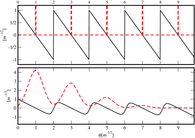
Figure 1: $\Upsilon(\phi|R,m)$ (full curve) and the probability of the of the stability $\mathcal{P}(\phi|m)$ (dashed curve) against $\phi$ in units of $1/\sqrt{m}$ for $R=1$ (upper panel) and $R=0.99$ (lower panel) for $m=9.$ Observe that for $R=1$ (upper panel) the average of the LHS (10) involves only the points at which $\Upsilon(\phi|1,m)$ is zero, whilst for $R<1$ (lower panel) the same average requires a more intensive calculation.

Observe that if $m=m_{\mathbf{B}},$ the second term of the RHS of (8) is zero, the algorithm applied is optimal and the overlap reaches $R^{\star}=1$ with the smallest possible set of examples. If perfect learning implies $R^{\star}=1$ it is natural to ask for what values of m the student can learn a teacher with dilution $m_{\mathbf{B}}$ without errors. From (4) and (5) we have that, for $R=1,$

$$\mathcal{P}(\phi|m_{\mathbf{B}}) = \frac{\sqrt{m_{\mathbf{B}}}}{2^{m_{\mathbf{B}}-1}}\sum_{k=0}^{(m_{\mathbf{B}}-1)/2}{m_{\mathbf{B}}\choose(m_{\mathbf{B}}-1)/2-k}\,\delta\left(\sqrt{m_{\mathbf{B}}}\,\phi-(2k+1)\right)$$ (11)

$$\Upsilon(\phi|1,m_{\mathbf{B}}) = \frac{1}{\sqrt{m_{\mathbf{B}}}}\left[1+\sum_{k=1}^{(m_{\mathbf{B}}-1)/2}\Theta\left(\sqrt{m_{\mathbf{B}}}\,\phi-2k\right)\right]-\phi$$ (12)

$$\Upsilon(\phi|1,m) = \frac{1}{\sqrt{m}}\left[1+\sum_{k=1}^{(m-1)/2}\Theta\left(\sqrt{m}\,\phi-2k\right)\right]-\phi.$$ (13)

The LHS of (10), averaged over (11) is zero (see figure 1). This is due to the fact that $\Upsilon((2k+1)/\sqrt{m_{\mathbf{B}}}|1,m_{\mathbf{B}})=0$. Therefore, in order to satisfy (10) we also need that $\Upsilon((2k+1)/\sqrt{m_{\mathbf{B}}}|1,m)=0$. Particularly, for $k=0$ these two equation imply that

$$\sqrt{\frac{m}{m_{\mathbf{B}}}} = 1+\sum_{k=1}^{(m-1)/2}\Theta\left(\sqrt{\frac{m}{m_{\mathbf{B}}}}-2k\right).$$

Therefore

$$\sqrt{\frac{m}{m_{\mathbf{B}}}}=2q+1,$$ (14)

where q is a suitable, non-negative integer. Thus, the condition for $R=1$ to be a solution of (10) is that there exist $q\in\mathbb{N}\cup\{0\}$ such that $m=(2q+1)^{2}m_{\mathbf{B}}.$

If this is not true, the solution of (10) is at $R^{\star}<1.$ We will present an approach based on the assumption that the root $R^{\star}$ occurs in a regime where the Gaussian distributions $\mathcal{N}(\phi|R^{\star}\mu_{k},1-R^{\star 2})$ in (4) and (5) have a small overlap. This could be ensured if the separation of two adjacent Gaussian components were larger than two standard deviations, i.e.

$$R^{\star}|\mu_{k}-\mu_{k+1}|=\frac{2R^{\star}}{\sqrt{m}} \gg 2\sqrt{1-R^{\star 2}}$$ (15)

$$1 \gg m\,\frac{1-R^{2}}{R^{2}}$$ (16)

At $R=1$ the curve $\Upsilon(\phi|1,m)$ is discontinuous at $\phi\equiv 2k/\sqrt{m}$ and the probability $\mathcal{P}(\phi|m)$ is a linear combination of delta functions centered at $\phi=(2k+1)/\sqrt{m}$ (upper panel of figure 1). For $R<1$ (figure 1, lower panel), $\Upsilon(\phi|R,m)$ is continuous and $\mathcal{P}(\phi|m)$ is a linear combination of Gaussian distributions centered at $\phi=R(2k+1)/\sqrt{m}$ with variance $1-R^{2}$. In both cases $\Upsilon(\phi|R,m)$ appears to be a periodic function of $\phi$ with period $\phi_{T}\equiv 2R/\sqrt{m},$ in the support of $\mathcal{P}(\phi|m)$ $\mathscr{D}_{\phi}\subset\mathbb{R},$ i.e.

$$\Upsilon(\phi|R,m) \simeq \Upsilon\left(\phi+n\phi_{T}|R,m\right),$$

and particularly for $R=1$ we have that

$$\Upsilon(\phi|1,m)=\sum_{\ell=0}^{(m-1)/2}\Theta\left[\left(2(\ell+1)-\sqrt{m}\,\phi\right)\left(\sqrt{m}\,\phi-2\ell\right)\right]\left(\frac{2\ell+1}{\sqrt{m}}-\phi\right).$$ (17)

We can approximate $\Upsilon(\phi|R,m)$ by a suitable superposition of Normal distributions. Consider the superposition

$$\tilde{\Upsilon}(\phi|R,m)\equiv\int_{-\infty}^{\infty}\mathrm{d}r\,g(r)\,\mathcal{N}(\phi|r,1-R^{2}).$$ (18)

To determine the function $g(r)$, we perform a variational calculation to minimize the error functional

$$\varepsilon[g]\equiv\frac{1}{2}\int_{\mathscr{D}_{\phi}}\mathrm{d}\phi\,\left[\Upsilon(\phi|R,m)-\tilde{\Upsilon}(\phi|R,m)\right]^{2}.$$

Observe that the optimal function $g_{o}(r)$ is the solution of the equation ${\displaystyle\left.\frac{\delta\varepsilon}{\delta g}\right|_{g_{o}}=0,}$ which implies that for all $r_{0}\in\mathbb{R}$ we have that

$$\int_{\mathscr{D}_{\phi}}\mathrm{d}\phi\,\left[\Upsilon(\phi|R,m)-\tilde{\Upsilon}(\phi|R,m)\right]\,\mathcal{N}(\phi|r_{0},1-R^{2})=0,$$

in particular if $R=1$ (we assume that $g_{o}(r)$ is independent of $R$)

$$0 = \int_{\mathscr{D}_{\phi}}\mathrm{d}\phi\,\left[\Upsilon(\phi|1,m)-\int_{-\infty}^{\infty}\mathrm{d}r\,g_{o}(r)\,\delta(\phi-r)\right]\,\delta(\phi-r_{0})$$

$$g_{o}(r_{0}) = \Upsilon(r_{0}|1,m)$$

Therefore

$$\Upsilon(\phi|R,m) \simeq \int_{\mathscr{D}_{\phi}}\mathrm{d}r\,\Upsilon(r|1,m)\,\mathcal{N}(\phi|r,1-R^{2})$$ (19)

$$= \sum_{\ell=0}^{(m-1)/2}\int_{2\ell R/\sqrt{m}}^{2(\ell+1)R/\sqrt{m}}\mathrm{d}r\,\left[(2\ell+1)\frac{R}{\sqrt{m}}-r\right]\,\mathcal{N}(\phi|r,1-R^{2})$$

$$= \frac{R^{2}}{m}\int_{-1}^{1}\mathrm{d}t\,t\,\sum_{\ell=0}^{(m-1)/2}\mathcal{N}(\phi|R(2\ell+1-t)/\sqrt{m},1-R^{2}).$$

Let us define the integral

$$\mathscr{I}_{m_{1},m_{2}} \equiv \int\mathrm{d}\phi\,\mathcal{P}(\phi|m_{\mathbf{B}})\,\Upsilon(\phi|R,m_{1})\,\Upsilon(\phi|R,m_{2}).$$ (20)

Following the development of Appendix C we have that

$$\mathscr{I}_{m_{1},m_{2}}\simeq 1-R^{2}\left[1-\frac{1}{2^{m_{\mathbf{B}}-1}}\sum_{k=0}^{(m_{\mathbf{B}}-1)/2}{m_{\mathbf{B}}\choose(m_{\mathbf{B}}-1)/2-k}\,\delta_{m_{1},k}^{\star}\delta_{m_{2},k}^{\star}\right],$$ (21)

where $\delta_{m_{j},k}^{\star}$ are given by

$$\delta_{m_{j},k}^{\star}=\frac{2}{\sqrt{m_{j}}}\,\left[\!\!\left|\sqrt{\frac{m_{j}}{m_{\mathbf{B}}}}\,\frac{2k+1}{2}-\frac{1}{2}\right|\!\!\right]+\frac{1}{\sqrt{m_{j}}}-\frac{2k+1}{\sqrt{m_{\mathbf{B}}}},$$ (22)

where $[\!|r|\!]$ is the closest integer to $r\in\mathbb{R}$.

Observe that from (8) we have that in the asymptotic regime

$$0 = 2\left\langle\Upsilon(\phi|R^{\star},m_{\mathbf{B}})\,\Upsilon(\phi|R^{\star},m)\right\rangle_{\phi|m_{\mathbf{B}}}-\left\langle\Upsilon^{2}(\phi|R^{\star},m)\right\rangle_{\phi|m_{\mathbf{B}}}$$

$$= 2\mathscr{I}_{m_{\mathbf{B}},m}-\mathscr{I}_{m,m}\,\,,$$

and observing that $\mathscr{I}_{m_{\mathbf{B}},m}=1-R^{2}$ (given that $\delta_{m_{\mathbf{B}},k}^{\star}=0\;\forall k$) and

$$\mathscr{I}_{m,m}=1-R^{2}+\frac{R^{2}}{2^{m_{\mathbf{B}}-1}}\sum_{k=0}^{(m_{\mathbf{B}}-1)/2}{m_{\mathbf{B}}\choose(m_{\mathbf{B}}-1)/2-k}\,\delta_{m,k}^{\star 2}$$

then

$$R^{\star 2} = \left[1+\frac{1}{2^{m_{\mathbf{B}}-1}}\sum_{k=0}^{(m_{\mathbf{B}}-1)/2}{m_{\mathbf{B}}\choose(m_{\mathbf{B}}-1)/2-k}\,\delta_{m,k}^{\star 2}\right]^{-1}$$ (23)

and observe that $\delta_{m,k}^{\star}=0$ iff $m=(2q+1)^{2}m_{\mathbf{B}},\;q\in\mathbb{N},$ which is consistent with (14).

III Numerical Results

Using (23) we plot $e_{g}^{\star}=e_{g}(R^{\star})$ as a function of $\sqrt{m/m_{\mathbf{B}}}$ (see figure 2).

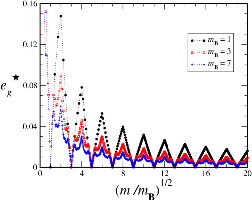
Figure 2: Generalization error in the asymptotic regime $e_{g}^{\star}$ as a function of $\sqrt{m/m_{\mathbf{B}}},$ for $m_{\mathbf{B}}=1,3,7$. We have use (23) to compute the overlap $R^{\star}$.

To validate our result shown in (23) we run a series of numerical experiments consisting of a student learning from a Teacher with only one bit ($m_{\mathbf{B}}=1$). The student updates its synaptic vector following (2) using a learning algorithm given by (6) with $m=1,3,\dots,N.$ To compute the generalization error we average over 50 realizations of the learning curve. The maximum number of examples considered was $16\,000.$ In figure 3 we present the $e_{g}$ as a function of $\alpha^{\frac{1}{4}}$ for $m=1,5,9,13,25,27$ and network size $N=51.$ We have chosen the exponent $\frac{1}{4}$ to better show the curve features at short times and the approach to the asymptotic regime. It is clear from the picture that for $m=1^{2},3^{2},5^{2}$ the generalization error for large $\alpha$ drops to zero as predicted. In order to extract the asymptotic behaviour of the curves we applied the Bulirsch-Stoer algorithm bs .

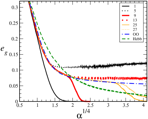
Figure 3: Generalization error as a function of $\alpha^{\frac{1}{4}}$, for a teacher with dilution $m_{\mathbf{B}}=1$ and students with $m=1,5,9,13,25,27$, for a network with $N=51$. The curves that corresponds to the Hebb algorithm ($F=1$, long dashed) and $m=\infty$ (dot dashed) are presented as a reference.

In figure 4 we present the extrapolated values of the learning curves together with the values estimated by the application of (23) as a function of $\sqrt{m}$. The error bars are estimates obtained also by the application of the Bulirsch-Stoer algorithm.

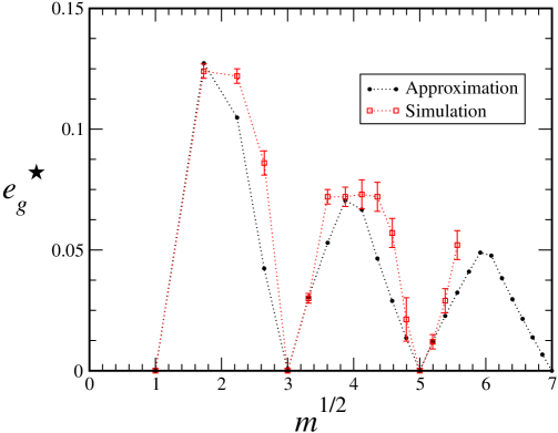
Figure 4: Comparison of the asymptotic value of the generalization error using (23) and the extrapolated values of the curves presented in figure 3.

IV Conclusions

We studied the generalization capabilities of a student optimally adapted for learning from a teacher B, when learning from a teacher $\mathbf{B}^{\prime}\neq\mathbf{B}.$ We observed that, although the algorithm the student uses may be suited for learning from a harder teacher, (as defined by Franco) that does not guarantee the success of the process, as revealed by (23). This behavior is due to the extreme specialization implied by the algorithm (6). When this algorithm (with parameter m) is applied to learn from a teacher with $m_{\mathbf{B}}<m$, the student tries to extract information from bits that the teacher does not use for producing the correct classification. These interference effects produce mostly bad results, originating a residual error in the asymptotic regime. In this sense, the algorithm $F_{\mathrm{op}}^{(m)}$ is worse than the Hebb algorithm $F_{\mathrm{Hebb}}=1.$

Despite the discrepancies shown in figure 4, our estimate (23) reproduces faithfully the qualitative behaviour observed in the simulations. There are two sources of uncertainty that may account for the observed discrepancies: the (finite) size of the network used and a not sufficiently large $\alpha.$

From figure 2, the algorithm obtained by taking the limit $m\to\infty$ in (6)

$$F_{\mathrm{op}}^{(\infty)}=\sqrt{\frac{Q\,\left(1-R^{2}\right)}{2\pi\,R^{2}}}\;\frac{\exp\left(-{\displaystyle\frac{1}{2}\,\frac{R^{2}\phi^{2}}{1-R^{2}}}\right)}{\mathcal{H}\left(-{\displaystyle\frac{R\phi}{\sqrt{1-R^{2}}}}\right)},$$

where $\mathcal{H}(x)=\int_{x}^{\infty}\mathrm{d}y\,\mathrm{e}^{-\frac{y^{2}}{2}}\,/\sqrt{2\pi}$; as reported by caki , produces zero residual error for all $m_{\mathbf{B}}$. The Hebb algorithm $F_{\mathrm{Hebb}}=1$ also produces learning curves with zero residual error. In figure 3 we observe that the Hebb algorithm performs better than $F_{\mathrm{op}}^{(\infty)}$. This is not a contradictory result. $F_{\mathrm{op}}^{(\infty)}$ is the algorithm that has the best average performance considering a homogeneous distribution of teachers over the N-sphere. For a measure zero subset of vectors embedded in the N-sphere, like the perceptrons with finite dilution m, $F_{\mathrm{op}}^{(\infty)}$ could perform worse than the Hebb algorithm, as it seems to be the case here.

In order to obtain the fastest decaying learning curve, a student has to infer the correct dilution of the teacher for choosing the appropriate learning algorithm. Developing an efficient technique for inferring the correct dilution parameter will be the subject of our future research.

Appendix A Distance sensitivity

S and $\mathbf{S}^{\prime}$ are vectors that differ in exactly P bits, i.e. $\sum_{j=1}^{P}\Theta(-S_{\sigma_{j}}S_{\sigma_{j}}^{\prime})=P$. Taken S as a reference, we can construct a Pth neighbor $\mathbf{S}^{\prime}$ by choosing without replacement P indexes from 1 to N and flipping the correspondent entries in S. There are ${N\choose P}$ different ways to choose P indexes, each one creating a different set of indexes $\mathbb{I}_{P}$. Introducing the scaled variables $\mu=\mathbf{w}\cdot\mathbf{S}/\sqrt{N}$ and $\mu^{\prime}=\mathbf{w}\cdot\mathbf{S}^{\prime}/\sqrt{N}$ by means of Dirac delta functions and adding up over all possible configurations S, we can express the discrepancy component as

$$\mathfrak{d}_{P}^{N}(\mathbf{B}^{(m)}) = {N\choose P}^{-1}{\int_{-\infty}^{\infty}}\frac{\mathrm{d}\mu\,\mathrm{d}{\hat{\mu}}}{2\pi}\,\frac{\mathrm{d}\mu^{\prime}\,\mathrm{d}{\hat{\mu}}^{\prime}}{2\pi}\,\Theta{\left(-\mu\mu^{\prime}\right)}\,\mathrm{e}^{-i\left(\mu{\hat{\mu}}+\mu^{\prime}{\hat{\mu}}^{\prime}\right)}$$ (24)

$$\qquad\qquad\sum_{\mathbb{I}_{P}}\prod_{j\in\mathbb{I}_{P}}\cos\left(\frac{\hat{\mu}-\hat{\mu}^{\prime}}{\sqrt{N}}B_{j}^{(m)}\right)\prod_{j\notin\mathbb{I}_{P}}\cos\left(\frac{\hat{\mu}+\hat{\mu}^{\prime}}{\sqrt{N}}B_{j}^{(m)}\right).$$

The fraction of sets $\mathbb{I}_{P}$ with $n\leq m$ indexes $\ell\leq m$ is ${m\choose n}{N-m\choose P-n}/{N\choose P}$ and observing that in the limit $P\leq N\to\infty$ with $P/N=p\leq 1$ we have that

$$\lim_{P\leq N\uparrow\infty}{N\choose P}^{-1}\,{N-m\choose P-n}=p^{n}(1-p)^{m-n}.$$

From equation (24) we have that

$$\mathfrak{d}^{(m)}(p) = {\int_{-\infty}^{\infty}}\frac{\mathrm{d}\mu\,\mathrm{d}{\hat{\mu}}}{2\pi}\,\frac{\mathrm{d}\mu^{\prime}\,\mathrm{d}{\hat{\mu}}^{\prime}}{2\pi}\,\Theta{\left(-\mu\mu^{\prime}\right)}\,\mathrm{e}^{-i\left(\mu{\hat{\mu}}+\mu^{\prime}{\hat{\mu}}^{\prime}\right)}$$

$$\times \sum_{n=0}^{m}{m\choose n}\,p^{n}(1-p)^{m-n}\,\cos\left(\frac{\hat{\mu}-\hat{\mu}^{\prime}}{\sqrt{m}}\right)^{n}\cos\left(\frac{\hat{\mu}+\hat{\mu}^{\prime}}{\sqrt{m}}\right)^{m-n}.$$

By adding up the sum, opening up the cosines and applying the identity $\Theta(ab)=\Theta(a)\Theta(b)+\Theta(-a)\Theta(-b),$ the expression for the sensitivity gets reduced to

$$\mathfrak{d}^{(m)}(p) =2 \sum_{n=0}^{m}{m\choose n}\,(1-2p)^{n}\left[\int\mathcal{D}(\mu,\hat{\mu})\,\cos(\hat{\mu}/\sqrt{m})^{m-n}\,\sin(\hat{\mu}/\sqrt{m})^{n}\right]^{2},$$

where the notation $\int\mathcal{D}(\mu,\hat{\mu})\,f(\mu,\hat{\mu})$ stands for $(2\pi)^{-1}\int_{0}^{\infty}\mathrm{d}\mu\int_{-\infty}^{\infty}\mathrm{d}\hat{\mu}\,\mathrm{e}^{-i\mu\hat{\mu}}\,f(\mu,\hat{\mu}).$ The integrals to be solved are

$$b_{0}^{m} \equiv \int\mathcal{D}\left(\eta,\hat{\eta}\right)\cos(\hat{\eta})^{m}$$

$$b_{n}^{m} \equiv \int\mathcal{D}\left(\eta,\hat{\eta}\right)\cos(\hat{\eta})^{m-2n}\sin(\hat{\eta})^{2n}$$

$$c_{n}^{m} \equiv \int\mathcal{D}\left(\eta,\hat{\eta}\right)\cos(\hat{\eta})^{m-(2n+1)}\sin(\hat{\eta})^{2n+1}.$$

Before computing the integrals observe that for all $A>0\;\mathrm{and}\;B\geq 0$

$$\int\mathcal{D}\left(\eta,\hat{\eta}\right)\sin(A\hat{\eta}) = -\frac{i}{4\pi}\int_{0}^{\infty}\mathrm{d}\eta\int_{-\infty}^{\infty}\mathrm{d}\hat{\eta}\exp\left(-i\hat{\eta}\eta\right)\left[\exp\left(i\hat{\eta}A\right)-\exp\left(-i\hat{\eta}A\right)\right]$$ (25)

$$= -\frac{i}{4\pi}\int_{0}^{\infty}\mathrm{d}\eta\int_{-\infty}^{\infty}\mathrm{d}\hat{\eta}\left[\exp\left[-i\hat{\eta}(\eta-A)\right]-\exp\left[-i\hat{\eta}(\eta+A)\right]\right]$$

$$= -\frac{i}{2}\left[\Theta(A)-\Theta(-A)\right]$$

$$= -\frac{i}{2},$$

similarly

$$\int\mathcal{D}\left(\eta,\hat{\eta}\right)\cos(A\hat{\eta})\cos(B\hat{\eta}) = \frac{1}{4}\left[\Theta(A+B)+\Theta(-A-B)+\Theta(A-B)+\Theta(-A+B)\right]$$ (26)

$$= \frac{1}{2}$$

and

$$\int\mathcal{D}\left(\eta,\hat{\eta}\right)\cos(A\hat{\eta})\sin(B\hat{\eta}) = -\frac{i}{4}\left[\Theta(A+B)-\Theta(A-B)+\Theta(-A+B)-\Theta(-A-B)\right]$$ (27)

$$= -\frac{i}{2}\Theta(B-A).$$

The first integral is (remember that m is odd)

$$b_{0}^{m} = \int\mathcal{D}\left(\eta,\hat{\eta}\right)\cos(\hat{\eta})^{m}=\frac{1}{2^{m-1}}\sum_{k=0}^{(m-1)/2}{m\choose k}\int\mathcal{D}\left(\eta,\hat{\eta}\right)\cos[(m-2k)\hat{\eta}]$$ (28)

$$= \frac{1}{2^{m}}\sum_{k=0}^{(m-1)/2}{m\choose k}=\frac{1}{2}.$$

The second integral is

$$b_{n}^{m} = \int\mathcal{D}\left(\eta,\hat{\eta}\right)\cos(\hat{\eta})^{m-2n}\sin(\hat{\eta})^{2n}$$ (29)

$$= \int\mathcal{D}\left(\eta,\hat{\eta}\right)\frac{1}{2^{m-2n-1}}\sum_{k=0}^{(m-1)/2-n}{m-2n\choose k}\cos[(m-2(k+n))\hat{\eta}]$$

$$\qquad\frac{1}{2^{2n}}\left\{2\sum_{j=0}^{n-1}(-1)^{n-j}{2n\choose j}\cos[(2n-2j)\hat{\eta}]+{2n\choose n}\right\}$$

$$= \frac{1}{2^{m-1}}\sum_{k=0}^{(m-1)/2-n}{m-2n\choose k}\,\sum_{j=0}^{n-1}(-1)^{n-j}{2n\choose j}+\frac{1}{2^{2n+1}}{2n\choose n}$$

$$= \frac{1}{2^{m-1}}\,\frac{2^{m-2n}}{2}\left[-\frac{1}{2}{2n\choose n}\right]+\frac{1}{2^{2n+1}}{2n\choose n}$$

$$= 0.$$

And the last integral is then

$$c_{n}^{m} = \int\mathcal{D}\left(\eta,\hat{\eta}\right)\cos(\hat{\eta})^{m-(2n+1)}\sin(\hat{\eta})^{2n+1}$$ (30)

$$= \int\mathcal{D}\left(\eta,\hat{\eta}\right)\cos(\hat{\eta})^{m-(2n+1)}\left[1-\cos^{2}(\hat{\eta})\right]^{n}\sin(\hat{\eta})$$

$$= \int\mathcal{D}\left(\eta,\hat{\eta}\right)\sum_{\ell=0}^{n}(-1)^{\ell}\,{n\choose\ell}\,\cos(\hat{\eta})^{m-(2n+1)+2\ell}\sin(\hat{\eta})$$

$$= \sum_{\ell=0}^{n}(-1)^{\ell}\,{n\choose\ell}\,\frac{(-i)}{2^{m-1+2(\ell-n)}}\left\{\frac{1}{2}\,{m-1+2(\ell-n)\choose(m-1)/2+\ell-n}+\right.$$

$$\qquad\left.+\sum_{k=0}^{(m-1)/2+\ell-n-1}{m-1+2(\ell-n)\choose k}\Theta\left[1-(m-1+2(\ell-n)-k)\right]\right\}$$

$$= -\frac{i}{2^{m-2n}}\sum_{\ell=0}^{n}\left(-\frac{1}{4}\right)^{\ell}\,{n\choose\ell}\,{m-1+2(\ell-n))\choose(m-1)/2+\ell-n}$$

$$= -\frac{i}{2^{m}}\,{2n\choose n}\,{m-1-2n\choose(m-1)/2-n}\,{(m-1)/2\choose n}^{-1}.$$

We have that, for all m odd

$$\mathfrak{d}^{(m)}(p)=\frac{1}{2}-\frac{1}{2}\sum_{n=0}^{(m-1)/2}a_{n}^{m}\,(1-2p)^{2n+1},$$ (31)

where

$$a_{n}^{m}\equiv\frac{1}{4^{m-1}}{\displaystyle\,{m\choose 2n+1}\,\left[{2n\choose n}\,{m-1-2n\choose(m-1)/2-n}\,{(m-1)/2\choose n}^{-1}\right]^{2}}.$$ (32)

Observe that $\mathfrak{d}^{(m)}(p)$ is concave in $p\in[0,\frac{1}{2}]$ (it is simply a sum of an affine plus concave functions) and $\mathfrak{d}^{(m)}(p)<\mathfrak{d}^{(m+2)}(p)$ for all $p\in(0,\frac{1}{2}).$ To demonstrate the latter we use that $\mathfrak{d}^{(m)}(0)=0$ and $a_{s}^{m}>0\;\forall s$. Thus, from (31) at $p=0$ we have that

$$\sum_{s=0}^{(m-1)/2}a_{s}^{m}=1\qquad\forall m\geq 1.$$ (33)

Therefore

$$a_{(m+1)/2}^{m+2} = \sum_{s=0}^{(m-1)/2}\left(a_{s}^{m}-a_{s}^{m+2}\right)$$

simply by applying (33) to $m$ and to $m+2$. Observe that $(1-2p)^{n}<(1-2p)^{n^{\prime}}$ for all $n>n^{\prime}$ and $p\in(0,\frac{1}{2})$, thus

$$a_{(m+1)/2}^{m+2}\,(1-2p)^{m+2} < \sum_{s=0}^{(m-1)/2}\left(a_{s}^{m}-a_{s}^{m+2}\right)\,(1-2p)^{2s+1}$$

$$\sum_{s=0}^{(m+1)/2}a_{s}^{m+2}\,(1-2p)^{2s+1} < \sum_{s=0}^{(m-1)/2}a_{s}^{m}\,(1-2p)^{2s+1}$$

and thus $\mathfrak{d}^{(m)}(p)<\mathfrak{d}^{(m+2)}(p)$.

In the large m limit we have that

$$\lim_{m\uparrow\infty}\mathfrak{d}^{(m)}(p)=\frac{1}{\pi}\mathrm{arcos}(1-2p),$$

which is the expected result feller .

Appendix B Optimal learning algorithm

The basic ingredient to compute the optimal learning algorithm is the joint probability distribution of the variables $\sigma_{\mathbf{B}}$, h and b. Given that $\mathcal{P}(\sigma_{\mathbf{B}},h,b|m)=\Theta(\sigma_{\mathbf{B}}b)\,\mathcal{P}(h,b|m)$ we will start our inference task by computing the distribution of the post-synaptic fields.

$$\mathcal{P}(h,b|m) = \left\langle\delta\left(h-\mathbf{J}\cdot\mathbf{S}/|\mathbf{J}|\right)\,\delta\left(b-\mathbf{B}\cdot\mathbf{S}/|\mathbf{B}|\right)\right\rangle_{\mathbf{S}}$$

$$= \int_{-\infty}^{\infty}\frac{\mathrm{d}\hat{h}}{2\pi}\,\mathrm{e}^{-i\hat{h}h}\int_{-\infty}^{\infty}\frac{\mathrm{d}\hat{b}}{2\pi}\,\mathrm{e}^{-i\hat{b}b}\left\langle\exp\left(i\hat{h}\frac{\mathbf{J}\cdot\mathbf{S}}{|\mathbf{J}|}+i\hat{b}\frac{\mathbf{B}\cdot\mathbf{S}}{|\mathbf{B}|}\right)\right\rangle_{\mathbf{S}}$$

and assuming that $[\mathbf{B}]_{j}=\sqrt{\frac{N}{m}}\,\Theta(m+1-j)$ we can suppose that the student learns this rule in such a way that $[\mathbf{J}]_{j}\simeq\mathcal{J}\Theta(m+1-j)+\varepsilon_{j},$ where $\varepsilon_{j}\ll|\mathbf{J}|$ are i.i.d. variables. Therefore

$$\frac{\mathcal{J}}{|\mathbf{J}|}=\frac{R}{\sqrt{m}}-\frac{\overline{\varepsilon}}{|\mathbf{J}|},$$

where R is the teacher-student overlap and $\overline{\varepsilon}\equiv\sum_{j=1}^{m}\varepsilon_{j}/m$. Let us define the variables

$$\varphi_{j}\equiv\frac{\varepsilon_{j}-\overline{\varepsilon}}{|\mathbf{J}|},$$

with the properties of $\sum_{j=1}^{m}\varphi_{j}=0$ and

$$\sum_{j>m}\frac{\varepsilon_{j}^{2}}{|\mathbf{J}|^{2}}=1-R^{2}-\sum_{j=1}^{m}\varphi_{j}^{2}.$$

Thus the trace over the spin variables gives

$$\left\langle\exp\left(i\hat{h}\frac{\mathbf{J}\cdot\mathbf{S}}{|\mathbf{J}|}+i\hat{b}\frac{\mathbf{B}\cdot\mathbf{S}}{|\mathbf{B}|}\right)\right\rangle_{\mathbf{S}} = \prod_{j=1}^{N}\frac{1}{2}\sum_{S=\pm 1}\exp\left[i\left(\frac{\hat{h}[\mathbf{J}]_{j}}{|\mathbf{J}|}+\frac{\hat{b}[\mathbf{B}]_{j}}{|\mathbf{B}|}\right)S\right]$$

$$= \prod_{j=1}^{m}\cos\left(\hat{h}\frac{\mathcal{J}+\varepsilon_{j}}{|\mathbf{J}|}+\frac{\hat{b}}{\sqrt{m}}\right)\,\prod_{j>m}\cos\left(\frac{\hat{h}\varepsilon_{j}}{|\mathbf{J}|}\right)$$

$$= \prod_{j=1}^{m}\cos\left(\frac{\hat{h}R+\hat{b}}{\sqrt{m}}+\hat{h}\varphi_{j}\right)\,\prod_{j>m}\cos\left(\frac{\hat{h}\varepsilon_{j}}{|\mathbf{J}|}\right)$$

$$\simeq \cos\left(\frac{\hat{h}R+\hat{b}}{\sqrt{m}}\right)^{m}\prod_{j=1}^{m}\left[1-\hat{h}\varphi_{j}\tan\left(\frac{\hat{h}R+\hat{b}}{\sqrt{m}}\right)+O\left(\varphi_{j}^{2}\right)\right]$$

$$\qquad\qquad\exp\left(-\frac{\hat{h}^{2}}{2}\sum_{j>m}\frac{\varepsilon_{j}^{2}}{|\mathbf{J}|^{2}}\right)\left[1+O\left(\sum_{j>m}\frac{\varepsilon_{j}^{4}}{|\mathbf{J}|^{4}}\right)\right]$$

$$\simeq \cos\left(\frac{\hat{h}R+\hat{b}}{\sqrt{m}}\right)^{m}\exp\left(-\frac{1-R^{2}}{2}\,\hat{h}^{2}\right)+O\left(\sum_{j=1}^{m}\varphi_{j}^{2}\right).$$

Therefore, and using that m is odd,

$$\mathcal{P}(h,b|m) \simeq \frac{1}{2^{m-1}}\sum_{k=0}^{(m-1)/2}{m\choose k}\int_{-\infty}^{\infty}\frac{\mathrm{d}\hat{h}}{2\pi}\,\frac{\mathrm{d}\hat{b}}{2\pi}\,\exp\left(-\frac{1-R^{2}}{2}\hat{h}^{2}-ih\hat{h}-ib\hat{b}\right)\cos\left[(m-2k)\frac{\hat{b}+R\hat{h}}{\sqrt{m}}\right]$$ (34)

$$= \mathcal{N}(h|Rb,1-R^{2})\,\frac{1}{2^{m}}\sum_{k=0}^{(m-1)/2}{m\choose(m-1)/2-k}\left[\delta\left(b-\mu_{k}\right)+\delta\left(b+\mu_{k}\right)\right],$$

where $\mu_{k}=(2k+1)/\sqrt{m}$ and $\mathcal{N}(x|\mu,\sigma^{2})$ is a Normal distribution in $x$, centered at $\mu,$ with variance $\sigma^{2}.$

From (34) we can compute the joint distribution of the variables h and $\sigma_{\mathbf{B}}$

$$\mathcal{P}(\sigma_{\mathbf{B}},h|m)=\frac{1}{2^{m}}\sum_{k=0}^{(m-1)/2}{m\choose(m-1)/2-k}\,\mathcal{N}(\sigma_{\mathbf{B}}h|R\mu_{k},1-R^{2}),$$ (35)

which implies that

$$\mathcal{P}(\phi|m) = \sum_{\sigma_{\mathbf{B}}=\pm 1}\int_{-\infty}^{\infty}\mathrm{d}h\,\mathcal{P}(\sigma_{\mathbf{B}},h|m)\,\delta(\phi-\sigma_{\mathbf{B}}h)$$ (36)

$$= \frac{1}{2^{m-1}}\sum_{k=0}^{(m-1)/2}{m\choose(m-1)/2-k}\,\mathcal{N}(\phi|R\mu_{k},1-R^{2}).$$

The conditional probability of the field b given $\sigma_{\mathbf{B}}$ and h can be obtained from (34) and (35).

It is a simple inference exercise to find the conditional distribution of the field b given the stability $\phi$

$$\mathcal{P}(b|\phi,m)=\frac{1}{2}\,\frac{\mathcal{N}(\phi|R|b|,1-R^{2})\sum_{k=0}^{(m-1)/2}{m\choose(m-1)/2-k}\delta(|b|-\mu_{k})}{\sum_{k=0}^{(m-1)/2}{m\choose(m-1)/2-k}\mathcal{N}(\phi|R\mu_{k},1-R^{2})}.$$

The conditional expectation of the field $|b|$ is

$$\left\langle|b|\right\rangle_{b|\phi,m} = \int_{-\infty}^{\infty}\mathrm{d}b\,|b|\,\mathcal{P}(b|\phi)$$ (37)

$$= \frac{\sum_{k=0}^{(m-1)/2}{m\choose(m-1)/2-k}\,\mu_{k}\,\mathcal{N}(\phi|R\mu_{k},1-R^{2})}{\sum_{k=0}^{(m-1)/2}{m\choose(m-1)/2-k}\,\mathcal{N}(\phi|R\mu_{k},1-R^{2})}.$$

Appendix C Derivation of (21)

In this Appendix we continue the development of (20)

$$\mathscr{I}_{m_{1},m_{2}} = \int\mathrm{d}\phi\,\mathcal{P}(\phi|m_{\mathbf{B}})\,\Upsilon(\phi|R,m_{1})\,\Upsilon(\phi|R,m_{2})$$

$$= \frac{1}{2^{m_{\mathbf{B}}-1}}\sum_{k=0}^{(m_{\mathbf{B}}-1)/2}{m_{\mathbf{B}}\choose(m_{\mathbf{B}}-1)/2-k}\,\sum_{\ell_{1}=0}^{(m_{1}-1)/2}\,\sum_{\ell_{2}=0}^{(m_{2}-1)/2}\frac{R^{4}}{m_{1}m_{2}}\,\int_{-1}^{1}\mathrm{d}t_{1}\,t_{1}\,\int_{-1}^{1}\mathrm{d}t_{2}\,t_{2}$$

$$\qquad\int\mathrm{d}\phi\,\mathcal{N}(\phi|R\mu_{k})\,\mathcal{N}\left(\phi\left|\frac{R}{\sqrt{m_{1}}}(2\ell_{1}+1-t_{1})\right.\right)\,\mathcal{N}\left(\phi\left|\frac{R}{\sqrt{m_{2}}}(2\ell_{2}+1-t_{2})\right.\right),$$

where all the Normal distributions have exactly the same variance $1-R^{2}$. The integral over $\phi$ is simple and produces a bi-variate Gaussian distribution in $t_{1}$ and $t_{2}$

$$\mathscr{I}_{m_{1},m_{2}} = \frac{1}{2^{m_{\mathbf{B}}-1}}\sum_{k=0}^{(m_{\mathbf{B}}-1)/2}{m_{\mathbf{B}}\choose(m_{\mathbf{B}}-1)/2-k}\,\sum_{\ell_{1}=0}^{(m_{1}-1)/2}\,\sum_{\ell_{2}=0}^{(m_{2}-1)/2}\frac{R^{2}}{\sqrt{m_{1}m_{2}}}$$ (38)

$$\quad\int_{\mathscr{D}_{\mathbf{t}}}\mathrm{d}\mathbf{t}\,t_{1}\,t_{2}\,\mathcal{N}\left(\mathbf{t}\left|\mathbf{t}_{\ell_{1},\ell_{2},k};\mathbf{\Sigma}\right.\right)$$

where $\mathbf{t}=(t_{1},t_{2})^{\mathsf{T}},$ $\mathscr{D}_{\mathbf{t}}\equiv(-1,1)\times(-1,1)$, $\mathbf{t}_{\ell_{1},\ell_{2},k}=(\sqrt{m_{1}}\,\delta_{\ell_{1},k},\sqrt{m_{2}}\,\delta_{\ell_{2},k})^{\mathsf{T}}$ and

$$\delta_{\ell_{j},k} \equiv \frac{2\ell_{j}+1}{\sqrt{m_{j}}}-\frac{2k+1}{\sqrt{m_{\mathbf{B}}}},$$ (39)

$$\mathbf{\Sigma} \equiv 2\,\frac{1-R^{2}}{R^{2}}\left(\begin{array}[]{cc}m_{1}&\frac{1}{2}\sqrt{m_{1}m_{2}}\\ \frac{1}{2}\sqrt{m_{1}m_{2}}&m_{2}\end{array}\right).$$ (42)

From (15) all the entries of the covariance matrix (42) are small, therefore all the distributions are concentrated around $\mathbf{t}_{\ell_{1},\ell_{2},k}.$ Let $\mathbf{t}_{k}^{\star}$ be the vector that corresponds to the largest term in (38). Its components are

$$\ell_{m_{j},k}^{\star} \equiv \left[\!\!\left|\sqrt{\frac{m_{j}}{m_{\mathbf{B}}}}\,\frac{2k+1}{2}-\frac{1}{2}\right|\!\!\right]$$ (43)

$$\sqrt{m_{j}}\,\delta_{m_{j},k}^{\star} = 2\ell_{m_{j},k}^{\star}+1-\sqrt{\frac{m_{j}}{m_{\mathbf{B}}}}\,(2k+1),$$ (44)

where $\left[\!\!\left|r\right|\!\!\right]$ is the closest integer to $r\in\mathbb{R}$, thus $\sqrt{m_{j}}\,\delta_{m_{j},k}^{\star}\in(-1,1)$. All the other vectors can be expressed as $\mathbf{t}_{\ell_{1},\ell_{2},k}=\mathbf{t}_{k}^{\star}+2\mathbf{n},$ where $\mathbf{n}=(n_{1},n_{2})^{\mathsf{T}},\,n_{j}=-\ell_{m_{j},k}^{\star},-\ell_{m_{j},k}^{\star}+1,\dots,-1,1,\dots,-\ell_{m_{j},k}^{\star}+(m_{j}-1)/2$. We have that

$$\mathscr{I}_{m_{1},m_{2}} = \frac{1}{2^{m_{\mathbf{B}}-1}}\sum_{k=0}^{(m_{\mathbf{B}}-1)/2}{m_{\mathbf{B}}\choose(m_{\mathbf{B}}-1)/2-k}\,\frac{R^{2}}{\sqrt{m_{1}m_{2}}}$$

$$\quad\left\{\int_{\mathscr{D}_{\mathbf{t}}}\mathrm{d}\mathbf{t}\,t_{1}\,t_{2}\,\mathcal{N}\left(\mathbf{t}\left|\mathbf{t}_{k}^{\star};\mathbf{\Sigma}\right.\right)+\sum_{\mathbf{n}}\int_{\mathscr{D}_{\mathbf{t}}}\mathrm{d}\mathbf{t}\,t_{1}\,t_{2}\,\mathcal{N}\left(\mathbf{t}\left|\mathbf{t}_{k}^{\star}+2\mathbf{n};\mathbf{\Sigma}\right.\right)\right\}.$$

Observe that the vectors $\mathbf{t}_{k}^{\star}$ are always strictly inside the domain $\mathscr{D}_{\mathbf{t}}$. They can never be in the boundary of the domain given that $m_{j}$ is odd then the argument of the RHS of (43) is never in $\mathbb{Z}_{1/2}$ (which would produce the largest possible value of $\sqrt{m_{j}}\,\delta_{m_{j},k}^{\star}$). Thus, the largest contribution to the sum over $\mathbf{n}$ is of $O\left[\exp\left(-\epsilon^{2}/\max\left\{\lambda\in\mathrm{spec}(\mathbf{\Sigma})\right\}\right)\right],$ where $\epsilon\sim 1-|\sqrt{m_{j}}\,\delta_{m_{j},k}^{\star}|>\frac{1}{2}$ and

$$\max\left\{\lambda\in\mathrm{spec}(\mathbf{\Sigma})\right\}=\frac{1-R^{2}}{R^{2}}\left[m_{1}+m_{2}+\sqrt{m_{1}^{2}+m_{2}^{2}-m_{1}m_{2}}\right]\ll 1,$$

according to (15). Within the same approximation error we can suppose that the centre of the zero-th Normal distribution is located inside the domain and sufficiently farther from the boundary. Thus

$$\mathscr{I}_{m_{1},m_{2}} \simeq \frac{1}{2^{m_{\mathbf{B}}-1}}\sum_{k=0}^{(m_{\mathbf{B}}-1)/2}{m_{\mathbf{B}}\choose(m_{\mathbf{B}}-1)/2-k}\,\frac{R^{2}}{\sqrt{m_{1}m_{2}}}\,\int_{\mathbb{R}^{2}}\mathrm{d}\mathbf{t}\,t_{1}\,t_{2}\,\mathcal{N}\left(\mathbf{t}\left|\mathbf{t}_{k}^{\star};\mathbf{\Sigma}\right.\right)+$$

$$\qquad+O\left(\exp\left[-\frac{\epsilon^{2}}{\max\left\{\lambda\in\mathrm{spec}(\mathbf{\Sigma})\right\}}\right]\right).$$

Thus

$$\mathscr{I}_{m_{1},m_{2}} \simeq \frac{1}{2^{m_{\mathbf{B}}-1}}\sum_{k=0}^{(m_{\mathbf{B}}-1)/2}{m_{\mathbf{B}}\choose(m_{\mathbf{B}}-1)/2-k}\,\frac{R^{2}}{\sqrt{m_{1}m_{2}}}$$

$$\quad\int_{-\infty}^{\infty}\mathrm{d}t_{2}\,t_{2\,}\mathcal{N}\left(t_{2}\left|\delta_{m_{2},k}^{\star};2m_{2}\frac{1-R^{2}}{R^{2}}\right.\right)$$

$$\qquad\int_{-\infty}^{\infty}\mathrm{d}t_{1}\,t_{1\,}\mathcal{N}\left(t_{1}\left|\delta_{m_{1},k}^{\star}+\frac{1}{2}\sqrt{\frac{m_{1}}{m_{2}}}\,(t_{2}-\delta_{m_{2},k}^{\star});\frac{3}{2}m_{1}\frac{1-R^{2}}{R^{2}}\right.\right)$$

$$= 1-R^{2}\left[1-\frac{1}{2^{m_{\mathbf{B}}-1}}\sum_{k=0}^{(m_{\mathbf{B}}-1)/2}{m_{\mathbf{B}}\choose(m_{\mathbf{B}}-1)/2-k}\,\delta_{m_{1},k}^{\star}\delta_{m_{2},k}^{\star}\right].$$

References

(1)D. E. Rumelhart and J. L. MacClelland, Parallel
distributed processing vol I, MIT Press, Cambridge, MA, 1986.
(2)M. Minsky and S. A. Papert, Perceptrons: An
Introduction to Computational Geometry, MIT Press, Cambridge, MA,
expanded edition, 1988/1989.
(3)A. Engel and C. Van den Broeck, Statistical
Mechanics of Learning, Cambridge Univ. Press, 2001.
(4)A. Church, Am. J. Math. 58, 345 (1936).
(5)A. M. Turing, Proc. London Math. Soc. 42,
230 (1937).
(6)J. Hartmanis and R. E. Stearns, Trans.
Am. Math. Soc.117, 285 (1965).
(7)A. N. Kolmogorov, Problems of Information
and Transmission 1, 1 (1965).
(8)M. Li and P. Vitányi, An introduction to Kolmogorov
Complexity and its Applications, 2nd edition, Springer, 1997.
(9)L. Franco and S. Cannas, Neural Computation 12,
2405 (2000).
(10)L. Franco and S. Cannas, Physica A332, 337 (2004).
(11)L. Franco and M. Anthony, Proc. of the IEEE Int. Joint
Conf. on Neural Networks (Budapest, Hungary) p 973, 2004.
(12)A. C. C. Coolen, R. Kühn and P. Sollich, Theory
of Neural Information Processing Systems, Oxford Univ. Press, 2005.
(13)A. Canning and E. Gardner, J. Phys. A 21,3275
(1988).
(14)M. Bouten, A. Engel, A. Komoda and R. Serneels, J.
Phys. A 23, 4643 (1990).
(15)D. Bollé and J. van Mourik, J. Phys. A 27,
1151 (1994).
(16)P. Kuhlmann and K. R. Müller, J. Phys. A 27,
3759 (1994).
(17)B. López and W. Kinzel, J. Phys. A 30,
7753 (1997).
(18)D. Malzahn, Phys. Rev. E 61, 6261 (2000).
(19)G. Kalai, Adv. in Appl. Math. 29, 412 (2002).
(20)R. W. O’Donnell, Computational Applications
of Noise Sensitivity, MIT Thesis, 2003.
(21)J. Stoer and R. Bulirsch, Introduction to numerical
analysis, Springer Verlag, New York, 1980.
(22)O. Kinouchi and N. Caticha, Phys. Rev. E 54,
R54 (1996).
(23)W. Feller, An Introduction to Probability Theory
and Its Applications, Second Edition, John Wiley, New York, 1957.