Multiband Hubbard Models and the Transition Metals

Abstract

Correlation computations on multiband Hubbard Hamiltonians are presented. It is shown why the proper degeneracy is of vital importance and that the atomic exchange interaction plays a particular role. The different methods are connected, and their results are discussed. Many experimental properties for the elemental solids can be explained by single closely related sets of parameters each. There is an exception, $T_{c}$ of $Fe$. Here, a novel feature of longer-range interactions enters. Connections are made to LSDA-calculations; and their seeming successes and deficiencies are explained.

I Introduction

A breakthrough in the understanding of the itinerant ferromagnetism of the $3d$-transition metals occured when density functional (DF) calculations, performed in the local density approximation (LDA) LDA1 ; LDA2 or rather its spin generalized variant, local spin density approximation (LSDA) 6 , obtained seemingly perfect values for the magnetic moments of the metals. Good results were also obtained for other ground state properties: binding energies, equilibrium volumes, bulk moduli, and Fermi surfaces, to name a few 15 ; 16 ; 17 .

A crucial aspect in this context is the behaviour of the $3d$-electrons. The $3d$-atomic orbitals are largely localized in space around the nuclei, and form rather narrow tight binding bands with a width of roughly 5eV. This localization is considerably stronger for the $3d$ than for the heavier $4d$ or $5d$-transition metals. In the following work, the consequences of this localization are investigated for the $3d$-transition metals.

While there have been many speculations about a full localization of the $3d$-electrons and about a representation of their degrees of freedom by spin-Hamiltonians, the delocalization is a feature that is strongly supported by experiment. Already before the success of LSDA, the experimental binding energies were unambiguously connected to delocalized $3d$-electrons 38 . In LSDA, the explicit part of the kinetic energy is obtained from a maximally delocalized single-determinant reference state while correlation corrections are contained in a functional. Consequently the former part represents the limit of maximal delocalization of the $3d$-electrons. On the other hand there is evidence that the LSDA results overemphasize binding by up to 20 percent 18 , possibly due to a mishandling of correlation corrections. This deviation in turn sets an upper limit to possible correlation corrections. In particular strong correlations or electronic degrees of freedom that can be described in terms of atomic moments are ruled out.

With the $3d$-electrons basically delocalized in tight-binding bands, magnetism must result from the electronic interactions. As already mentioned, these cannot be so strong that localized atomic moments arise. Even more, it needs to be understood why the LSDA is apparently able to handle these interactions that are definitely connected to the spatially strongly localized atomic orbital representation of the $3d$-elctrons. It is hard to imagine how a homogeneous-electron gas exchange-correlation potential can adequately deal with such inhomogeneous atomic features. In fact it cannot.

Bare local Coulomb-interaction matrix elements between electrons in these atomic orbitals are of the order of 20eV, far larger than the kinetic energy gained from delocalization into bands. Therefore, a second problem is to understand how these bare interactions are reduced into the required smaller interactions.

The optimal way to deal with these questions would be a full ab-initio correlation calculation. The only method available for such a treatment is the Local Ansatz (LA) stol3 ; stoln . It starts from Hartree-Fock (HF) ab-initio calculations for solids and adds correlations in a variational way like Quantum Chemistry (QC) methods do. However, it differs from these methods by using specifically constructed subsets of correlation operators with a well defined local meaning instead of trying to cover the whole correlation space in an orthogonal representation. This results in a loss of typically one to a few procent of the correlation energy in a given basis, but it leads to a large gain in efficiency and it enables the LA to treat metals. First ab-initio calculations for metals li and for a metallic transition metal compound s98 have already been performed, and calculations for non-magnetic transition metals are under way sun ; however, a complete coverage of the magnetic problem has not yet been obtained. Therefore, the problems mentioned above could so far only be addressed using correlation calculations for models.

The minimal level of complexity for such models is well defined: a tight-binding Hamiltonian for the $3d$-electrons, i.e. a five-band (per spin) Hamiltonian. The hope is that the $4s$- and $4p$-orbitals of the transition metals do not need to be explicitly included for the basic understanding of magnetism, since they contribute little to the electronic density of states in the relevant energy range around the Fermi energy. This omission certainly causes defects, for example of the Fermi surface. For the interactions, a first choice is the inclusion of only local (atomic) interactions of the $3d$-electrons. It is known that these can be condensed into three Slater parameters. We will in the following rearrange those terms and call the resulting interactions Hubbard ($U$) interaction, Hunds rule exchange terms ($J$), and anisotropy terms ($\Delta J$) 11 . The underlying assumption is that longer range contributions of the Coulomb interaction are almost perfectly screened for these metals.

Such models have for long been the basis of attempts to understand the itinerant ferromagnetism. However, these attempts were mostly restricted to simplified single-band models and/or to the approximate treatment of the interaction in Hartree-Fock (HF) approximation, or when the treatment was extended to finite temperatures within a functional integral formulation, to an equivalent static approximation. For an early overview, I refer to mor1 .

Here, the LA led to a sizeable improvement. Since it can be applied to models as well as to ab-initio calculations, we were able to perform satisfactory correlation calculations for the model described above, and we have computed the non-magnetic st as well as the magnetic os cases. The tool to understand the magnetic phase transition for the case of delocalized electrons is the Stoner-Wohlfarth theory sto ; wo . Such an analysis had been earlier performed in the case of LSDA computations gunn1 . We also analysed our results in the same way os85 ; soh , and managed to work out why the LSDA calculations had been so successful for the transition metals but had failed for a set of transition metal compounds soh ; soh1 . We abstained from any attempts to generalize the treatment of the order parameter beyound a mean-field (or Stoner-Wohlfarth) approximation. It should be noted that for the simplified handling of the interaction in HF or static approximation, a generalized spin fluctuation theory is available mor2 .

It turned out from our analysis that the 5-fold degeneracy of the model bands is very relevant. Single-band or two-band models are not able to catch the essence of the $3d$-magnetism at all. Many of the degeneracy features also are lost when restricting to a HF or static approximation. As will be shown below, a reduction of the degeneracy would require also larger and larger interactions and would incorrectly push the treatment into a strong-correlation direction which is inadequate for the $3d$-transition metals.

Five band models have been rarely treated by other methods beyound HF-approximation. A first attempt was made in the context of an insufficient second-order perturbation computation 35 ; 36 . Quasiparticle calculations followed using the Kanamori t-matrix approach 62 for almost filled degenerate band systems such as $Ni$ 58 ; 59 ; 60 ; 61 . Recently, calculations have been performed for nine-band models starting from an $R=0$-approximation that had also been used with the Local Ansatz but employing a full Configuration Interaction (CI) calculation instead of the weak-correlation expansion or of a two-particle excitation CI calculation both within the LA web ; web1 . Finally, the Dynamical Mean-Field-Theory (DMFT) has been used for such a model li2 . The latter is the appropriate generalization of the functional integral schemes just mentioned, and goes beyound the static approximation.

We will in the following introduce the five-band model plus its interactions, and describe in detail the LA treatment and the different approximations made. We will also establish connections to the other computational schemes.

In a next step, results of the calculations for the non-magnetic case will be presented, and the different approximations will be tested. A further step is to compute and analyse the magnetic results for $Fe$, $Co$, and $Ni$. Based on them, conclusions with regarding the comparability to experiment and assessing the specific deficiencies of the LSDA and its results will be made.

Finally, connections between the model and first ab-initio correlation results will be made, and the limits of the Hubbard-model scenario will be revealed.

II Model Hamiltonian and Single-Particle Groundstate

The aim of the qualitative treatment is to understand the delocalization and interaction of the $3d$-electrons which is the expected key for the understanding of magnetism in the 3d-elemental solids. There are five $3d$ electrons per spin and site (atom). A compact description of their delocalization is in the form of canonical d-bands jep . This is essentially a tight-binding description and has the additional advantage of containing only a single open parameter, namely the $3d$-band width $W$. The single-particle part of the model Hamiltonian ($H_{0}$) is given in terms of these orbitals in eigenvalue representation. In the computations, these bands are constructed for the two relevant lattices, bcc and fcc.

For these electrons we further assume that they only interact when they are on the same atom $l$. These interactions can be given in terms of three Slater interactions; here we choose a slightly different but equivalent notation. The full Hamiltonian $H$ reads

$$H = H_{0}+H_{1}$$ (1)

$$H_{0} = \sum_{\nu\sigma{\bf k}}e_{\nu}({\bf k})n_{\nu\sigma}({\bf k})$$ (2)

$$H_{1} = \sum_{\bf l}H_{1}({\bf l})$$ (3)

$$H_{1}({\bf l}) = {1\over 2}\sum_{ij\sigma\sigma}U_{ij}a_{i\sigma}^{\dagger}(l)a_{j\sigma^{\prime}}^{\dagger}(l)a_{j\sigma^{\prime}}(l)a_{i\sigma}(l)$$ (5)

$$+{1\over 2}\sum_{ij\sigma\sigma}J_{ij}[a_{i\sigma}^{\dagger}(l)a_{j\sigma^{\prime}}^{\dagger}(l)a_{i\sigma^{\prime}}(l)a_{j\sigma}(l)+a_{i\sigma}^{\dagger}(l)a_{i\sigma^{\prime}}^{\dagger}(l)a_{j\sigma^{\prime}}(l)a_{j\sigma}(l)].$$

The $e_{\nu}({\bf k})$ represent the five ($\nu=1..5$) canonical bands, and the $n_{\nu\sigma}({\bf k})$ the corresponding number operators of the Bloch eigenstates, whose creation and annihilation operators are $c_{\nu\sigma}^{\dagger}({\bf k}),c_{\nu\sigma}({\bf k})$. The $U_{ij}$ and $J_{ij}$ are the local (atomic)interaction matrices and related by

$$U_{ij}=U+2J-2J_{ij},$$ (6)

where $U$ and $J$ are the average Coulomb and exchange interaction constants. The matrix $J_{ij}$ contains the third interaction parameter $\Delta J$ that is a measure of the difference between the $e_{g}$ and $t_{2g}$ interactions. For details of this matrix, we refer to 11 ; os . For $\Delta J=0$, it holds that $J_{ij}=J$. The interactions are expressed in terms of the five local $3d$-orbitals $i$ on atomic positions $l$ whose creation and annihilation operators are given as $a_{i\sigma}^{\dagger}(l)a_{i\sigma}(l)$.

The size of these parameters will be fixed later. Typically, it holds that the band width $W$ that scales the single-particle part $H_{0}$ is roughly 5eV. The interactions are reduced to a single free parameter by setting $J\simeq 0.2U$ and $\Delta J\simeq 0.2J$. For $U$ it holds that typically $U\simeq 0.5W$.

Starting point of the following correlation treatment is the solution to the single-particle Hamiltonian $H_{0}$, called $\Psi_{0}$. This is written as

$$|\Psi_{0}(n_{d},0)\rangle=\prod_{{{\bf k}\nu\sigma}\atop{e_{{\bf k}\nu}\leq e_{F}(n_{d})}}c_{\nu\sigma}^{\dagger}({\bf k})|0\rangle.$$ (7)

This solution differs slightly from the self-consistent field (SCF) solution of the full model Hamiltonian $H$. The latter generates additional selfconsistently obtained crystal field terms that may lead to charge redistributions between the $e_{g}$ and $t_{2g}$ orbitals. However, since the interactions are not too large, and the original site occupations are almost degenerate, these redistributions can be almost neglected. An exception that will be discussed later is the case of ferromagnetic $Ni$ where the second requirenment does not hold. Such a solution is found for all fillings $n_{d}$ per atom of the five-band system, with $n_{d}$ ranging from 0 to 10. $e_{F}(n_{d})$ is the occupation dependent Fermi energy.

In addition to this non-magnetic solution, magnetic solutions with a moment $m$ are constructed by generating states

$$|\Psi_{0}(n_{d},m)\rangle=\prod_{{{\bf k}\nu}\atop{e_{{\bf k}\nu}\leq e_{F}(n_{d}+m)}}\prod_{{{\bf k^{\prime}}\nu}\atop{e_{{\bf k^{\prime}}\nu}\leq e_{F}(n_{d}-m)}}c_{\nu\uparrow}^{\dagger}({\bf k})c_{\nu\downarrow}^{\dagger}({\bf k^{\prime}})|0\rangle.$$ (8)

Here, the majority band with spin up is occupied with ${n_{d}+m\over 2}$ electrons, and the minority band with spin down with ${n_{d}-m\over 2}$. This ansatz is a rigid band approach. Again, a self-consistent solution might lead to small charge redistributions in the minority and majority bands if these are not empty or filled, respectively.

The Fermi energy for the individual cases like $Fe,Co,Ni$ is chosen so that the maximal magnetic moment agrees with the same one of the LSDA calculations. This implies an occupation of 7.4, 8.4, 9.4 for $Fe,Co$ and $Ni$, respectively. It is known from more careful charge analyses that the true atomic $3d$-occupations are somewhat smaller. For $Fe$ for example they amount to 6.5. Consequently, the $d$-orbitals of this model Hamiltonian are not maximally localized $3d$-tight binding orbitals but their tails have small $4s$-, $4p$-contributions.

III Correlated Ground State

III.1 Deficiencies of the Single-Particle Ground State

The single-particle ground state $\Psi_{0}$ is an eigenstate of the single-particle part of the Hamiltonian but results in a poor coverage of the interaction part. Being represented by eigenfunctions in momentum space, this state has maximal local charge fluctuations that are uncorrelated for the different bands. A measure of these charge fluctuations is the atomic quantity $\Delta n^{2}$ for a given wave function. It is given as

$$\Delta n^{2} = \langle\Psi|n^{2}(l)|\Psi\rangle-\langle\Psi|n(l)|\Psi\rangle^{2}$$ (9)

$$n(l) = \sum_{i\sigma}n_{i\sigma}(l),$$ (10)

where $n_{i\sigma}(l)$ is the density operator for an electron with spin $\sigma$ in orbital $i$ on site $l$.

For the single-particle ground state, it holds that

$$\Delta n^{2}(\Psi_{0}(n_{d},0)) = \sum_{i\sigma}n_{i\sigma}(1-n_{i\sigma})$$ (11)

$$n_{i\sigma} = \langle\Psi_{0}|n_{i\sigma}(l)|\Psi_{0}\rangle.$$ (12)

These fluctuations increase linear with the number of bands. For the half-filled five-band case with degenerate occupation we find that $\Delta n^{2}=2.5$. Correspondingly, the interaction energy costs per atom of this state in comparison to the disordered atomic limit amount to $1.25(U-{2\over 9}J)$. This needs to be compared to a kinetic energy gain which, for a roughly constant density of state, equals $-1.25W$. This indicates that half the delocalization energy is lost in this approximation for a ratio $U\simeq 0.5W$. However, the electrons on the individual atoms order by Hund’s rule and can gain an energy of $-{70\over 9}J$ at half-filling. Consequently, even for this relatively modest screened interaction, the solid is no longer bound in single-particle approximation and a better treatment is required, i.e. the correlated ground state needs to be computed. Without including correlations explicitly, any broken symmetry, even disordered local moments, would be favourable.

III.2 The Local Ansatz

For a three-dimensional model with five degenerate bands, the correlation treatment can not be done exactly but only approximately. Since the parameter choice lets us expect that the electrons are not too strongly correlated, the natural approach is to start from the single-particle ground state and add correlations as corrections.

This is how the Local Ansatz is set up. Here, the following variational ansatz is made for the correlated ground state:

$$|\Psi_{corr}\rangle = e^{-S}|\Psi_{0}\rangle$$ (13)

$$S = \sum_{\nu}\eta_{\nu}O_{\nu}$$ (14)

$$O_{\nu} = \left\{\matrix{n_{i\uparrow}(l)n_{i\downarrow}(l)\cr n_{i}(l)n_{j}(l^{\prime})\cr\vec{s}_{i}(l)\cdot\vec{s}_{j}(l^{\prime})\cr}\right.$$ (15)

The $n_{i\sigma}(l)$ and $\vec{s}_{i}(l)$ are density and spin operators for an electron in the local orbital $i$ on site $l$. The operators have a straightforward interpretation. For example, the first operator $n_{i\uparrow}(l)n_{i\downarrow}(l)$, when applied to $|\Psi_{0}\rangle$, picks out all configurations with two electrons in orbital $i$. When applied with a variational parameter $\eta_{\nu}$, as in eq.(13), it partially suppresses those configurations. For a single-band Hubbard model, such an ansatz was first made by Gutzwiller 33 . Similarly, the operators $n_{i}(l)n_{j}(l^{\prime})$ introduce density correlations between electrons in local orbitals $i,j$ either on the same site or on different sites $l,l^{\prime}$. The wave function generated by these two sets of operators, when applied to the homogeneous electron gas problem, is the Jastrow function jastr . The operators $\vec{s}_{i}\cdot\vec{s}_{j}$ generate spin correlations. On the same site, they introduce Hund’s rule correlations, while when applied for different sites they result in magnetic correlations.

For the same sites, all these operators are directly connected to $H_{1}$. They allow to correct exactly those features that are addressed by the interacton terms.

In the following, we will no longer use the full operators but only their two-particle excitation contributions. The standard approximation to derive the energy and to obtain the variational parameters is an expansion in powers of $\eta$, up to second order,

$$E_{G} = E_{SCF}+E_{corr}$$ (16)

$$E_{corr} = -2\sum_{\nu}\eta_{\nu}\langle O^{\dagger}_{\nu}H\rangle+\sum_{\mu\nu}\eta_{\nu}\eta_{\mu}\langle O^{\dagger}_{\nu}HO_{\mu}\rangle_{c}\ \ .$$ (17)

When optimizing this energy, the following equations arise that determine the energy and the variational parameters.

$$E_{\rm corr} = -\sum_{\nu}\eta_{\nu}\langle O^{\dagger}_{\nu}H\rangle$$ (18)

$$0 = -\langle O^{\dagger}_{\nu}H\rangle+\sum_{\mu}\eta_{\mu}\langle O^{\dagger}_{\nu}HO_{\mu}\rangle_{c}\ \ .$$ (19)

Here, $\langle A\rangle$ is the expectation value of the operator $A$ within $|\Psi_{0}\rangle$, and $\langle\rangle_{c}$ indicates that only connected contributions are included. It holds that $E_{SCF}=\langle H\rangle$ These equations can also be identified as a Linearized Coupled Cluster expansion, restricted to particular two-particle (double) and one-particle (single) excitations, abbreviated LCCSD. The concept of CC-equations was introduced into many-body physics and into Quantum Chemistry a long time ago cc1 ; cc2 ; cc3 ; cc4 . In the presented calculations on models, single-particle excitations were, in contrast to the ab-initio calculations, not included in the correlation treatment itself, but were covered by direct modifications in the trial single-particle wave functions.

The full treatment of these equations poses no problems, in particular when the operators are restricted to on-site terms. Then, without consideration of intrinsic symmetries, one has 5 Gutzwiller-like operators and 10 density and spin operators each. The most expensive step is the solution of a set of linear equations with dimension 25.

III.3 The $R=0$-Approximation and Alternatives to the Local Ansatz

The correlation calculations can be performed in a further approximation in which one may go beyond the LCCSD-equations. This approximation applies only when restricting to on-site operators. In this case one can approximately set all those terms in the matrices $\langle OH\rangle$ and $\langle OHO\rangle$ equal to zero where the operators in the $O$ or in $H_{1}$ are not on the same site. In this approximation, the full correlation treatment separates into independent contributions covering a single site each in an non-correlated and non-interacting environment. This approximation is called single-site or $R=0$-approximation. It was introduced for the first time in a second-order perturbation treatment of a five-band Hamiltonian that is very similar to the one used here. There, however, no restriction to a particular choice of correlation operators was made but the full two-particle operator space was covered 36 . In the single-site approximation of the LA, all required terms are simply obtained from two sets of single-particle elements, the individual occupations $n_{i\sigma}$ and the average energies on these sites, $e_{i\sigma}$, given as

$$e_{i\sigma}=\int_{-\infty}^{e_{F}}en_{i\sigma}(e)de$$ (20)

where $n_{i\sigma}(e)$ is the local partial density of state for orbital $i$ with spin $\sigma$. More details can be found in refs. st ; os . All terms that are left out in the single site approximation contain non diagonal density matrix elements of the form $P_{ij}(l,l^{\prime})=\langle a_{i}^{\dagger}(l)a_{j}(l^{\prime})\rangle$ with $R=l-l^{\prime}\neq 0$, explainng the name. With rising number of nearest neighbors, these contributions shrink in weight and disappear for the limit of infinitely many neighbors (or equivalently dimensions $d$). The approximation was therefore more recently called the $d=\infty$-approximation vo .

In a way, this approximation represents the correlation generalization of an approximate coherent potential approximation (CPA) where a single-site mean-field calculation with broken symmetry is performed which leads to disordered local moments. With on-site correlations properly included, a broken symmetry result does no longer arise, at least not prior to a Mott-Hubbard transition. Or, in different words, disordered local moments are a poor man’s approach to correlations.

This single-site approximation allows a more general treatment than the LCCSD-approximation. One possibility is to perform a $CI$-calculation for this single site. The exact energy of the variational state with two-particle excitations included is obtained. It represents a lower limit to the exact result, while the LCCSD-approximation usually overshoots the latter. The correlated wave function for the single site $l$ is defined as

$$|\Psi_{corr}(l)\rangle=(1-\sum_{\nu\in l}O_{\nu})|\Psi_{0}\rangle.$$ (21)

Its exact energy is

$$E_{G}(l) = E_{SCF}+E_{corr}(l)$$ (22)

$$E_{corr}(l) = {{-2\sum_{\nu}^{\prime}\eta_{\nu}\langle O^{\dagger}_{\nu}H^{\prime}\rangle+\sum_{\mu\nu}^{\prime}\eta_{\nu}\eta_{\mu}\langle O^{\dagger}_{\nu}H^{\prime}O_{\mu}\rangle_{c}}\over{1+\sum_{\mu\nu}^{\prime}\eta_{\nu}\eta_{\mu}\langle O^{\dagger}_{\nu}O_{\mu}\rangle_{c}}}\ \ .$$ (23)

Here, the $\sum^{\prime}$ indicates a restriction of the summation to operators on site $l$, and $H^{\prime}=H_{0}+H_{1}(l)$. When optimizing this energy, the resulting equations that determine the energy and the variational parameters can be written in close similarity to the LCCSD-equations 18,19.

$$E_{\rm corr}(l) = -\sum_{\nu}^{\prime}\eta_{\nu}\langle O^{\dagger}_{\nu}H^{\prime}\rangle$$ (24)

$$0 = -\langle O^{\dagger}_{\nu}H^{\prime}\rangle+\sum_{\mu}^{\prime}\eta_{\mu}\langle O^{\dagger}_{\nu}H^{\prime}O_{\mu}\rangle_{c}$$ (25)

$$+\sum_{\mu}^{\prime}\eta_{\mu}\langle O^{\dagger}_{\nu}O_{\mu}\rangle_{c}\sum_{\mu^{\prime}}^{\prime}\eta_{\mu^{\prime}}\langle H^{\prime}O_{\mu^{\prime}}\rangle_{c}\ \ .$$

The newly added terms in eq. 25 are responsible for the difference. One may generalize in this approximation and perform a full $CI$-calculation not restricted to two-particle operators. The system of equations (21,23,24,25) stays the same, but the operators $O_{\nu}$ are not restricted to two-particle excitations. The available operator space explodes exponentially with degeneracy, and the numerical demands rise sharply, but recently even nine-band models could be addressed this way (i.e., the $3d$- plus the $4s$- and $4p$-orbitals were included)web ; web1 .

An even more extended approach is to perform an exact calculation for the single site problem, based on dynamically fluctuating disordered local moments, called DMFT (for an introduction of its origins, see ref. vo ). This computation is based on a Green’s function formalism, and is the by far most expensive method. Formally, the operator space is extended beyond strictly local operators. Not all electrons are covered equally but their treatment is influenced by their individual energies. Applications to a nine-band model were done for $Fe$ and $Ni$ li2 using this method. A further advantage of this scheme is that quasiparticle results can be obtained and a transition to thermodynamic quantities is possible, since the computations are performed on a Green’s function level.

Let’s return to the most simple scheme, the LA. In contrast to the other methods, it cannot be applied to the Mott-Hubbard transition. However, it is the only scheme that can be extended beyond $R=0$ and can treat finite dimension corrections. Furthermore, it can deal with long range interactions, and even manage ab initio calculations with the full interaction.

There is actually a rather simple extension of the LA that makes it more tolerant of stronger correlations. This is the application of the full CCSD-equations. They arise from a full equation-of-motion of the original ansatz for the wave function, and not from a weak-coupling approximation. The resulting equations read as

$$E_{\rm corr} = -\sum_{\nu}\eta_{\nu}\langle O^{\dagger}_{\nu}H\rangle$$ (26)

$$0 = -\langle O^{\dagger}_{\nu}H\rangle+\sum_{\mu}\eta_{\mu}\langle O^{\dagger}_{\nu}HO_{\mu}\rangle_{c}$$ (27)

$$-{1\over 2}\sum_{\mu\mu^{\prime}}\eta_{\mu}\eta_{\mu^{\prime}}\langle O^{\dagger}_{\nu}HO_{\mu}O_{\mu^{\prime}}\rangle_{c}\ \ .$$

This generalization would improve the results for larger ratios of ${U\over W}$. When applied to a single-band Hamiltonian in the $R=0$-approximation, the result should, with single-particle operators properly added, reproduce the Gutzwiller approximation stohei .

III.4 Error Estimates of the different Approximations in the Local Ansatz

In the present treatment of the LA, three approximations are made that need to be controlled.

The first is the weak-correlation approximation. It may be tested by a comparison of the LCCSD- and the CI-result in the $R=0$-approximation.

The second is the $R=0$-approximation itself. It can be tested only in the weak-correlation approximation.

The last is the restriction in correlation operator space. Again, this will be tested in the weak correlation expansion.

The last restriction is best tested for the one-dimensional single-band Hubbard model. Here, the exact energy is known, and also its weak-correlation limit. The corresponding Gutzwiller ansatz which contains only single-site operators yields 92 percent of the exact correlation energy in this limit for the half-filled case. A large fraction of the missing energy can be obtained by longer-range density and spin correlations.

The situation is worse for almost empty bands. Here, additional correlation operators of the form $[H_{0},O_{\nu}]$ are required for a satisfactory result. Such operators do not open new correlation channels but allow us to take into account the band energies of the electrons involved in the correlation process. Such operators are included in the ab initio scheme and have turned out to be important in a different context stoln . We have found for the non-magnetic five-band calculations st ; s85 that these operators do not lead to noticable changes. Although being of non-local nature, such operators contribute in the $R=0$-approximation and bridge the difference between a correlation calculation restricted to local correlation operators and a DMFT calculation.

For the five-band model, we had also included nearest neighbor operators in the non-magnetic calculations st . The energy gain due to these terms was only a few percent; thus we can trust the results of calculations restricted to on-site correlations for the five-band Hamiltonian.

The $R=0$-approximation depends on the number of neighbors. For a two-site problem with a single orbital each, the $R=0$-result is only half the correct result. For the one-dimensional Hubbard model, the $R=0$ result needs to be enhanced by 33 percent to obtain the final LA result with on-site operators for half-filling, but already nearest neighbor or $R=1$-corrections reduce the deficiency to one percent. For the five-band problems treated here, the $R=1$-corrections turned out to be 2-3 percent for fcc or bcc, respectively st . Most of our calculations and all calculations for the magnetic state were therefore restricted to the $R=0$-approximation. On the other hand, these results indicate that an $R=0$ or $d_{\infty}$-approximation should not be applied to systems with less than six neighbors.

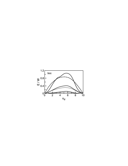
Figure 1: Several energies in units of $W$ as a function of band filling $n_{d}$. The interaction energy costs in SCF-approximation are given by the dashed line. The top full line gives the MP2 correlation result, the second full line the LCCSD-result, and the dotted line just below it the CI-result. The lowest full line and the dotted line below give the amount of correlation energy that is lost when the spin correlation operators are omitted from the LCCSD or CI calculations, respectively. All correlation calculations were performed for the bcc case and in the $R=0$-approximation (from ref. st ).

Let us finally turn to the validity of the weak-correlation approximation. It will definitely fail around half-filling for ratios ${U\over W}>1$. In Fig. 1, correlation energies in the $R=0$-approximation are given for a ratio of $U=0.5W$. The dashed curve gives the $HF$-energy costs $\Delta E_{SCF}=E_{SCF}-\langle H_{0}\rangle$. The topmost curve gives the result of a correlation calculation performed in second-order perturbation (MP2) expansion (the LCCSD-equation can be reduced to MP2 by replacing $\langle OHO\rangle$ by $\langle OH_{0}O\rangle$). This result overshoots the HF-term and is definitely wrong. The second solid curve gives the final result in LCCSD, and the dotted curve below it gives the CI-result. The maximal relative difference around half-filling amounts to 25 percent. When considering that the CI-result is a true lower limit, then the LCCSD-result should not overshoot the correct result by more than 5 percent. The lowest curves display the energies that are lost when spin-correlations are omitted. Here, the relative differences between CI and LCCSD are considerably larger but again the true result is expected to be close to the LCCSD result.

These particular features are closely connected to the degeneracy. As mentioned before, fluctuation costs arise in five channels $i$ in the HF-approximation. The correlation ansatz, however, makes 15 density correlation channels $i,j$ available. Thus, treating these channels independently as is done in perturbation theory, very soon overscreens the fluctuations. The term $H_{1}$ in $\langle OHO\rangle$ by which the LCCSD-equations differ from MP2 guarantees that the different channels take note of each other and act coherently. This distribution of correlation corrections among many different states also makes it plausible why the CI and LCCSD results are so close to each other although five degenerate orbitals need to be treated.

For the spin correlations, the situation is different. Here each pair $i,j$ can gain an interaction energy $J$ independent of each other. This is reproduced in the LCCSD-equations, while it is a particular feature of the CI-calculations restricted to two-particle excitations that at each moment one has either the one or the other electron pair corrected. Thus, the different contributions, also the spin and density contributions actually impede each other, and a considerably smaller energy is obtained. This explains why the largest part of the difference between the two schemes in the full calculation arises from the addition of the spin correlations. On a CI-level, this deficiency might only be corrected by including in the variational ansatz for the CI-wave function not only two-particle excitations but also their products, and finally up to ten-particle excitations.

The failure of MP2 found here is related to the failure of this approximation when the screening of the long-range Coulomb interactions in metals is concerned. There, fluctuations are also diagonal, i.e. connected to the local sites $l$. The correlation space, however, offers $l,l^{\prime}$ density correlations that are independent in MP2 and cause the well-known divergence of the correlation energy. The LCCSD scheme used here does not result in a divergence, but it is not perfect either. It generates only half of the screening of the long-range charge fluctuatons stohei .

The weak-correlation expansion used here looks very simple, but this is not at all the case when evaluated in a diagrammatic representation. In the linear equations 17,19, the interaction is included in both sets of terms. In a diagram representation, this means that infinite orders of diagrams are summed up. The LCCSD-approximation includes the Tamm-Dancoff approximation plus all related exchange diagram corrections and also contains the Kanamori limit. It does not yet contain the RPA-limit (plus all exchange corrections). The RPA-limit is covered by the full CCSD-equations in eqs.26, 27.

These findings also explain why reliable Green’s function results for the transition metals are rare. Only the almost empty or filled band cases, i.e. the Kanamori limit 58 ; 59 ; 60 ; 61 , have been easily accessible. For the case of Fe, one has been restricted to MP2-calculations that are more or less empirically renormalized un ; lic . Only the DMFT has made a significant progress by the use of large scale Monte Carlo computations li2 .

IV Results for the non-magnetic Ground State

IV.1 Ground State Energies

In the last section, some specific total energy contributions have been analyzed. Here, we will discuss them in more detail. The results discussed represent the bcc-case, and the ratio ${U\over W}={1\over 2}$ is used. Also $\Delta J$ is disregarded in the qualitative discussion for simplicity.

All total energies are related to an average interaction energy of electrons with the same occupation with localized electrons and without Hund’s rule ordering:

$$E_{0}(n_{d})=(U-{2\over 9}J)n_{d}(n_{d}-1).$$ (28)

The Hund’s rule energy gain for the ordered atoms is then

$$E_{atom}(n_{d}) = -{7\over 18}J\tilde{n}_{d}(\tilde{n}_{d}-1),\quad\mbox{where}\ \tilde{n}_{d}=\left\{\matrix{n_{d}\quad\mbox{for}\quad n_{d}\leq 5\cr(10-n_{d})\quad\mbox{for}\quad n_{d}\geq 5\cr}.\right.$$ (29)

The occupation dependence of this energy is shown in Fig. 2 (upper full line). It is strongly peaked at $n_{d}=5$.

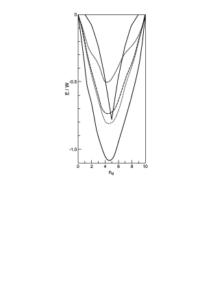
Figure 2: Energies for various approximations of the ground state in powers of $W$ as a function of band filling $n_{d}$ for the bcc case. The upper solid line represents the atomic energy, the lowest solid line the kinetic energy. The upper broken line represents the HF-energy, the lower broken line the result with density correlations included, and the dotted line the final LA result.

It is compared to the ground state energy for $H_{0}$ that is contained in the figure as the lowest solid line. This figure indicates the binding due to the $3d$-electron delocalization. Disregarding slight shifts, the difference between these two extremal curves is a good representation of the LDA binding energy contributions of the $3d$-electrons. This can be seen when comparing Fig. 2 with the LDA binding energy figure 1.1 in ref. 18 . Two corrections should be made. The first one is that the real atoms have occupations differing from the solids ($Fe$-atom, $n_{d}=6$ versus $n_{d}=7.4$ in the model), and the second one is that the bands are narrower for the heavier elements. By setting $W=5eV$, a typical binding of $2.5eV$ arises.

The upper broken curve in Fig. 2 represents the HF-energy. As already mentioned, half of the band energy gain is lost. Even worse, the uncorrelated ground state is no longer binding in the occupation range from 4 to 7. The situation is corrected when the full correlation treatment is performed (dotted curve). The correlated ground state is always bound, although only marginally at half-filling. This is in rough agreement with experiment, where the d-orbital contributions to the binding in $Mn$ are not larger than 1eV. Actually, the difference between the non-interacting and the fully correlated result matches roughly the difference between the LSDA and experimental binding energies for these cases (see again Fig. 1.1 in ref 18 ), and might well explain it, as will be discussed later. The figure also contains the energy when spin correlations are omitted (lower broken curve). As can be seen, the contributions of the spin correlations to the total energy are not large but nevertheless important.

IV.2 Correlation Functions

From our calculations, local correlation functions for the transition metals were obtained for the first time. The effects of the correlations are large, and should be basically experimentally accessible was not it for the yet lacking spatial resolution of x-rays, and for the too small energies of the neutrons. But it is still valuable to discuss a few theoretical results. The first correlation function is the atomic charge fluctuation $\Delta n^{2}$. The reduction of this quantity due to correlations is shown in Fig.3.

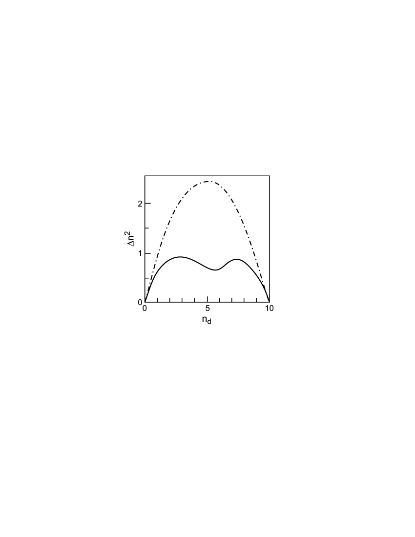
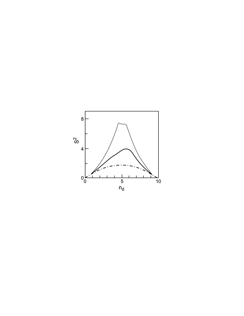
Figure 3: Left figure:Charge fluctuations as function of d-band filling $n_{d}$ (bcc). Upper curve without correlations, lower curve with correlations included
Right figure: Local spin correlations $S^{2}$ as function of d-band filling $n_{d}$ (bcc). Upper curve: Atomic limit, lower curve:SCF-result. Full line: LA-result (both from ref. st ).

As can be seen, it is sizable, although the electrons are not strongly correlated. This is due to the many available correlation channels. Wenn turning to the spin correlation function $S^{2}$, one has to be aware that the autocorrelation of the electrons leads to a finite value even in the uncorrelated state. This is given as the lower broken line in the right part of Fig. 3. Of importance is also the fully localized limit whose values of $S^{2}$ are given as the dotted line in this figure. The correlation result is given as the full line. As can be seen, spin correlations are strong but significantly smaller than in the localized limit. They are almost halfways in-between, the relative change being 0.45, almost independent of band filling. This also indicates that the proximity of the energy to the atomic limit at half-filling (see Fig. 2) does not yet cause a resonance-like correlation enhancement.

This presence of relatively strong spin correlations poses the question whether these can be treated in a good approximation as quasi-local moments, whether they for example already require a different timescale, or whether these correlations decay as fast as the electrons move, and only form a polarization cloud around the moving electrons.

The answer cannot be directly obtained from ground state calculations. There is, however, an indirect way to address this question, where one includes short-range magnetic correlations into the LA-calculation. There is no direct neighbor interaction in the Hamiltonian. Thus, a strong magnetic neighbor correlation would indicate the formation of local moments, at least in cases when the non-magnetic ground state is only metastable, and a ferromagnetic ground state exists. The calculation can be easily done by adding neighbor spin operators to the correlation treatment. This rules out a $R=0$-approximation. In the required computation, all matrix elements $P_{ij}(0,l)$ with $l$ nearest neighbors are included, and all nearest neighbor correlations are added up s85 .

The discussion of the obtained quantities requires some care because the non magnetic ground state is a singlet. This implies that the positive magnetic correlation function on the same site must be compensated by short-range antiferromagnetic correlations in order to obtain $S_{tot}^{2}|\Psi_{i}\rangle=0$, no matter whether the single particle (i=0) or correlated (i=corr) ground state is concerned. Neighbor antiferromagnetic correlations have therefore no relevance as such, but only their eventual changes due to added degrees of freedom are of relevance. Consequently, we compare for every filling the change in correlation with the maximal possible change, namely the local moment formation. We discuss therefore the quantity

$$\Delta S^{2}_{\delta}={{C(\delta)-C_{0}(\delta)}\over{S^{2}_{loc}-S^{2}_{0}}}.$$ (30)

Here, it holds that

$$C(\delta) = \langle\Psi_{corr}|S(l)S(l+\delta)|\Psi_{corr}\rangle$$ (31)

$$C_{0}(\delta) = \langle\Psi_{0}|S(l)S(l+\delta)|\Psi_{0}\rangle.$$ (32)

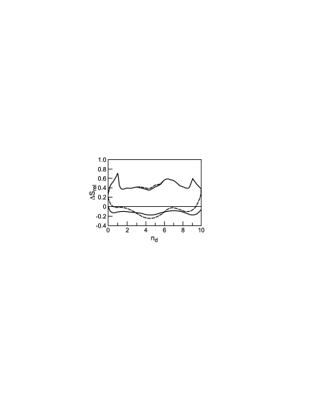
Figure 4: Relative change of the spin correlation function as function of band filling. Upper curves Change of on-site correlations, lower curves change of neighbor correlations. Full lines without neighbor correlations, broken curves with neighbor correlations added (from ref. s85 )

.

Fig. 4 displays these relative changes. In the upper part, the relative change of the on site spin correlation is given, in the lower part the one of the neighbor functions. The solid line displays the result without neighbor correlations that had just been discussed. The upper curve indicates on the average 45 percent of the maximal correlation, and the lower curve indicates the required antiferromagnetic re-ordering due to the on-site correlations in the neighbor function. This calculation was performed for the bcc case. As can be seen, the ratio is a little smaller than ${1\over 4}$. Therefore, additional longer range compensation effects are expected. The most interesting result is the changes due to added neighbor correlations. The resulting curves are given in Fig. 4 as dotted lines. These changes are very small. However, it is interesting that they recover the expected trends correctly. They indicate a tendency towards antiferromagnetism only around half-filling (from occupations of $3.5<n_{d}<6.5$). Apparently, the magnetic susceptibilities are slightly enhanced for the proper magnetic ordering. However, the moments themselves do not change at all, except around half-filling. Here, the stability of the non-magnetic state is smallest, as discussed above. It should be noted that for this choice of parameters, the stable ground state is ferromagnetic for band fillings of $n_{d}>7.0$.

To conclude, on-site correlations on neighbor atoms do not support each other. Barely noticable neighbor correlations form. These results strongly contradict a local moment assumption. The energy gain due to the added operators is small, it amounts to less than 100K per atom for Fe. Consequently, the strong on-site correlations cannot be interpreted as quasi-static local moments. Magnetic ordering restricted to nearest neighbors does not exist in these compounds. If magnetic order exists - and it must exist - then only for domains considerably larger than a single atom and its neighbors. This demonstrates again that the electrons in the transition metals are delocalized, and that spin fluctuations can only exist for small moments $q$, as experiments demonstrate (the stiffness constant of $Fe$, for example allowes magnetic excitations with energies smaller than $T_{c}$ only for moments $q$ smaller than one fifth of the Brioullin zone).

If there is really a need to adress i.e. the strong magnetic scattering above $T_{c}$ for $Ni$ 52 by methods extending beyond a critical Stoner-enhancement that was computed in ref. cstei , then this can only be done by long-range spin or order parameter fluctuation theories 54 ; 55 ; 53 .

IV.3 Compton Scattering

While experiments have not yet been able to provide informations about correlation functions, they have succeeded for another quantity that displays correlation effects: the density distribution in momentum space, $n({\bf k})$. The scattering intensity $I({\bf q})$ measured in Compton-scattering is given by the integral over all densities $n(\bf k)$ with ${\bf kq=q^{2}}$. The variation in $I({\bf q})$ with direction ${\bf q}$ provides a direct measure of the anisotropy of the Fermi surface c1 . These experimental results are in good qualitative agreement with Fermi surfaces obtained in LSDA for $Cu$ c1 , $Va$c2 ; c3 , $Cr$c3 , and $Ni$c4 with exception of a constant scaling factor. For $Fe$c5 ; c6 , the agreement is less good.

This constant scaling factor provides a measure of the correlation correction. In the single-particle approximation, all states with energies smaller than the Fermi energy are filled and the others are empty. This implies a maximal step at $n({\bf k_{F}})$. This result is changed by correlations. The changes are qualitatively depicted in the left part of Fig. 5.

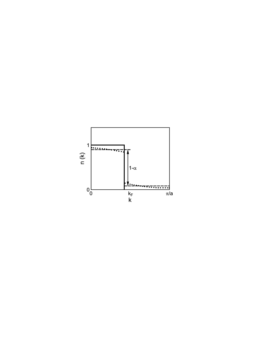
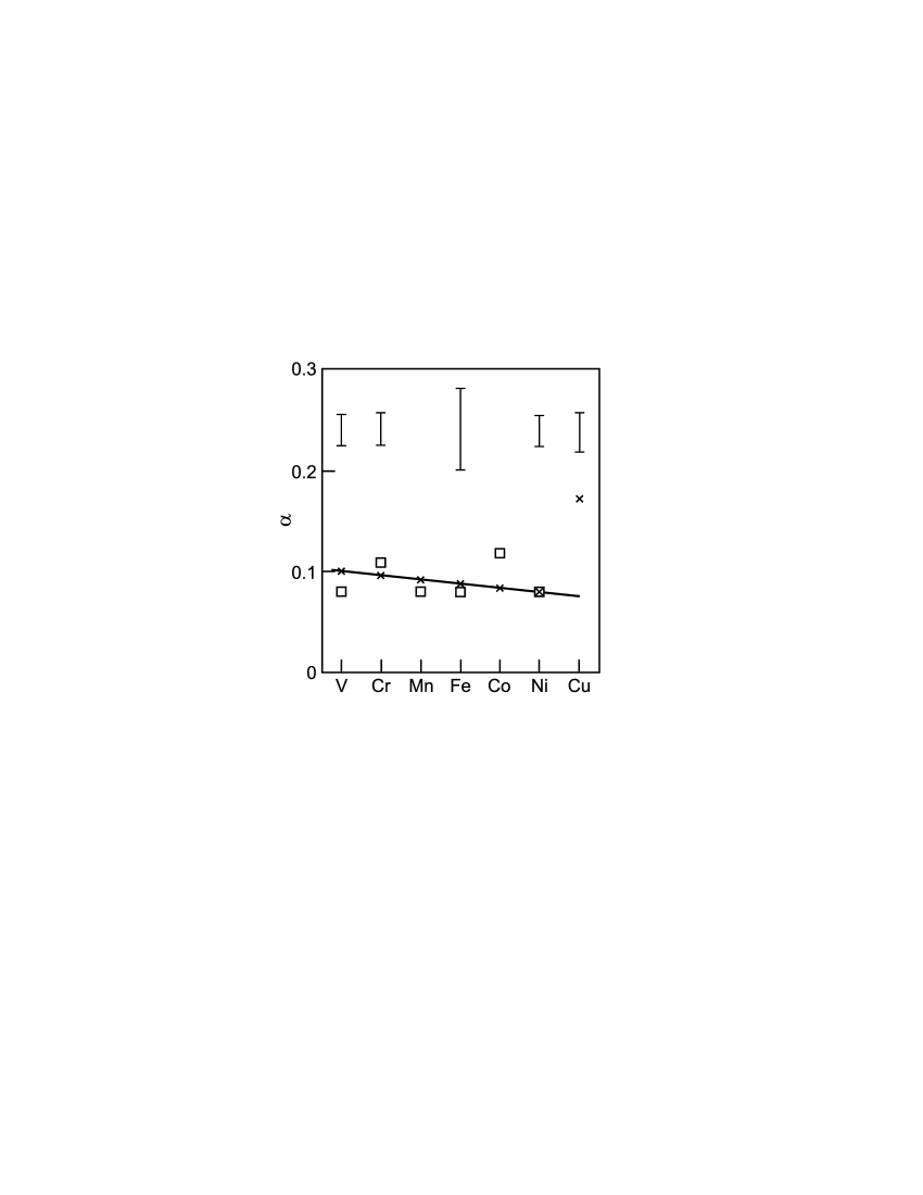
Figure 5: Left figure:Qualitative picture of changes in occupation around the Fermi energy due to correlations. Dots represent the real behaviour, and the dotted line the average change.
Right figure: Values of the quantity $\alpha$ in the left figure for different transition metals. The bars represent the values deduced from experiment in comparison to LSDA-results. Crosses give an homogeneous electron gas estimate $a_{hom}$, and squares give the contributions $\alpha_{LA}$ due to the atomic correlations of the screened d-electrons alone to this value taken from s952 .

For simplicity let us assume that correlations cause a constant shift $\alpha$ in occupations for the occupied and unoccupied parts of the partially filled bands. Then this correction $\alpha$ can be directly extracted from the scaling factor by which experiments (correlations included) and single-particle calculations (no correlations included) differ.

Fig. 5 (right part) contains the values for $\alpha$ for the mentioned transition metals and for $Cu$ as deduced from experiment. As can be seen this reduction amounts to 20-25 $\%$ in all cases.

This reduction $\alpha$ can be compared to its counterpart $\alpha_{hom}$ obtained for a homogeneous system with the same average density. For its derivation, we refer to c1 ; s952 . When taking for $Cu$ a single valence electron only (i. e. considering the d-electrons as part of the core), then the experimental value is regained. This indicates that as far as this property is concerned, the 4s (and 4p) electrons correlate as a homogeneous system of the same average density. For the transition metals, on the other hand, the d-electrons need to be incorporated into the estimate. The resulting $r_{s}$ value is much smaller than in the case of $Cu$ which implies - within the theory of the homogeneous electron gas - a smaller reduction of the occupation. The latter amounts to less than half of the correlation effects determined experimentally.

Within our scheme, the reduction $\alpha_{LA}$ is obtained from the change of the expectation value of $H_{0}$, the so-called kinetic or band energy, with correlations. For the uncorrelated ground state, it holds that

$$E(band)_{0}=\langle\Psi_{o}|H_{0}|\Psi_{0}\rangle=\sum_{\nu\sigma}\int_{e_{\nu}({\bf k})\leq e_{F}(\sigma)}d^{3}{\bf k}e_{\nu}({\bf k})$$ (33)

while the band energy of the correlated ground state is

$$E(band)=\langle\Psi_{corr}|H_{0}|\Psi_{corr}\rangle=(1-\alpha_{LA})E(band)_{0}$$ (34)

because the model Hamiltonian is constructed such that $Tr(H_{0})=0$. Thus, the quantity $\alpha_{LA}$ also represents the relative change of the band or kinetic energy of the model by correlations. For the magnetic cases, the values for the magnetic ground state are selected. The interaction parameters are chosen so that they correspond to the actual transition metals. The values found indicate again that the electrons are weakly correlated. Only 10 percent of the kinetic energy is lost due to atomic correlations.

The restriction to this model implies that only a part of the correlation corrections $\alpha$ can be obtained, i.e. the one which arises from the atomic correlations due to the strongly screened atomic d-electron interactions. The contributions of the screening itself to the momentum density, for example, are not included in this estimate. As can be seen from Fig. 5, the particular atomic correlation contributions $\alpha_{LA}$ alone as derived from the model computations are as large as the total homogeneous electron gas values $\alpha_{hom}$. Therefore, they must to a large extent be neglected in a homogeneous electron gas approximation as was explained before. They amount to almost half the experimental value $\alpha$ and can therefore explain the largest part of the deficit of a homogeneous electron gas treatment.

Correlations are included in a homogeneous electron gas approximation when LSDA calculations are performed. Such calculations must therefore lack a satisfactory description of these atomic correlations for the case of the transition metals.

V Results for the magnetic Ground State

V.1 Parametrization of the Hubbard Hamiltonian

Of main interest in the case of the magnetic transition metals is the magnetic moment itself. So far, for Hubbard models the interaction parameters were always chosen such that the experimental magnetic moment was obtained. It is an indication for the accuracy of the different discussed correlation treatments that these parameters are now closely related. Global differences for the most typical value $U+2J$ are not larger than 10 percent, and are connected with band structure differences between 5-band and 9-band models. This holds true as long as the interaction is restricted. When also interactions on and between the $4s,4p$-orbitals are included, then the $3d$-interaction also needs to be enhanced and the screening of the latter interaction by the $4s,4p$-electrons is explicitly covered.

The values for $W$ and $U$ for our model are given in table 1 together with the moment used.

	$Fe$	$Co$	$Ni$
$n$	7.4	8.4	9.4
$m$	2.1	1.6	0.6
$W$	5.4	4.8	4.3
$U$	2.4	3.1	3.3

Table 1: Parameters for our model (energies in eV) (from ref.os ).

In all cases, the ratio $J=0.2*U$ was kept. Only for the case of $Fe$ was $U$ unambiguously determined from the magnetic moment. In the other cases we had only lower limits which were 2.6 and 3.1eV for $Co$ and $Ni$, respectively. Below, we will present a comparison between the values of $U$ obtained here, and the ones obtained from other sources.

V.2 Dependence of Magnetism on Degeneracy

The degeneracy of the energy bands of the transition metals is of vital importance for magnetism itself, and also imposes strict boundary conditions on the possible treatments. To explain this, the magnetic energy gain and its magnetic moment dependence are analysed as a function of the represented method $i$ for the actual moment $m_{0}$.

$$\Delta E_{i}(m_{0})=E_{i}(m_{0})-E_{i}(0).$$ (35)

This energy gain as a function of magnetization is rewritten in the following form

$$\Delta E_{i}(m_{0})={1\over 4}\int_{0}^{m_{0}^{2}}D(m)dm^{2}-{1\over 4}\int_{0}^{m_{0}^{2}}I_{i}(m)dm^{2}.$$ (36)

Here, the first term describes the loss in (non-interacting) band or kinetic energy. It holds that

$$D(0)={1\over n(E_{F})}$$ (37)

is the inverse total density of states per spin at the Fermi energy. Its generalization for finite m is simple and can be found in ref. soh . The second part describes the interaction energy gain and is defined by this function. It is a generalized Stoner parameter. The optimal magnetic moment in approximation $i$ is defined by the condition

$$D(m_{0})=I_{i}(m_{0}).$$ (38)

For $m_{0}=0$, this is the standard Stoner criterion, and the Stoner parameter $I_{i}$ is the limiting $I_{i}(O)$. For a system with orbital degeneracy $N$ and a Hubbard interaction in the form of eq. 5, it holds in HF-approximation

$$I_{SCF}(M)={1\over N}(U+J(N+1)).$$ (39)

If we assume a structureless density of states with a bandwidth $W$, then $D(0)={W\over N}$, and for the single band model the Stoner criterion in SCF-approximation reads $U+2J=W$. In a single-band Hamiltonian, the interaction terms are usually condensed into a single $U$, but for the degeneracy treatment we will stay in our notation. Ferromagnetism in a single-band system can therefore only be expected for a strong interaction with $U\geq W$ where correlations are important. Correlations however strongly diminish $I$ from $I_{SCF}$, and shift the onset of magnetism to an even larger interaction. Thus, if spurious magnetism due to peaks in the density of states is disregarded, itinerant magnetism with large moments and weak correlations can arise only for highly degenerate systems. This is why we could obtain magnetism for 5-band systems with rather weak interactions of ${U\over W}\geq 0.5$. The atomic exchange interaction $J$ is the relevant quantity in this respect, and it requires an adequate treatment. Note that for the case with the smallest interaction, $Fe$, magnetism is strongly supported by a peak in the density of states, and that $Fe$ does not become fully magnetic.

We had already mentioned that the treatment of degenerate band systems puts strong additional demands on the many-body methods used. This also is the case for magnetic properties. Fig. 6 contains, for the bcc $Fe$-case, the correlated Stoner Parameter I(0) as a function of interaction $U$, renormalized by the SCF-Stoner parameter (roughly $(U+6J)$) to $\bar{I}$. For $U$=0, $\bar{I}(0)$ is therefore equal to 1, and it decreases due to correlation corrections.

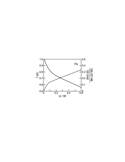
Figure 6: $I(0)$ as depending on the ratio ${U\over W}$ for Fe. In addition, the logarithmic deviation is given (from ref.soh ).

As can be seen, there is first a fast decrease, but then, at ${U\over W}=0.1$, a rigorous slowing down of the screening occurs. From the logarithmic derivative it can be seen that the exponent changes from 2 to ${1\over 2}$. This is the point where a second-order perturbation treatment is no longer sufficient, and a better approach is necessary.

Due to these experiences we decided to include in this review neither contributions that used false degeneracies nor contributions that are unable to treat degenerate systems well. Therefore, we did not cover work that is based on MP2 or lowest order diagram techniques. Besides the LA only the full $CI$-method given in refs web ; web1 , Kanamori t-matrix applications, and the first full applicaton of the DMFT to the transition metals li2 remained.

V.3 Magnetic Energy Gains, Stoner Parameter and $T_{c}$

Besides the moment that was taken from experiment, the most basic ground state quantity connected with the broken symmetry is the magnetization energy gain $\Delta E$.

	$Fe$	$Co$	$Ni$
$\Delta E_{HF}[eV]$	0.56	0.43	0.12
$\Delta E_{corr}$	0.15	0.13	0.03
$\Delta E_{LSDA}$	0.28	0.10	0.08
$T_{c}(LSDA)[K]$	4400	3300	2900
$T_{c}(DMFT)$	2000		700
$T_{c}(exp)$	1040	1400	631

Table 2: Magnetic energy gain in the HF-approximation and for the correlated ground state os and from LSDA calculations gunn1 . Stoner-transition temperatures from LSDA calculations gunn1 and DMFT li2 and the experimental transition temperatures.

The values of the energy gain are given in table 2 for our calculations in the single-particle approximation, for the full treatment of correlations, and for LSDA-calcluations gunn1 . A comparison of $\Delta E_{HF}$ and $\Delta E_{corr}$ shows how correlations reduce the magnetization energy gains. Be aware that the interactions employed are already strongly reduced screened interactions. When comparing the model and LSDA magnetic energy gains, then the LSDA quantities come out twice as large for $Fe$ and $Ni$. Without caring for any specific dependences on details of the density of states, this would imply a corresponding reduction in the Stoner $T_{c}$. An exception is the case of $Co$ but here we had possibly chosen a model interaction that was too large for reasons explained below.

The differences between the LA and the LSDA results can be understood by a discussion of the Stoner parameter $I(m)$. In the SCF-approximation, it holds for the degenerate band case

$$I_{SCF}(m)={1\over 5}(U+6J).$$ (40)

(the terms $\Delta J$ are disregarded). $I_{SCF}$ is independent of magnetization. The function $\Delta E_{LSDA}$ contains the same expression for the kinetic energy as the quantities defined above because in this approximation the uncorrelated kinetic energy of the reference wave function is used, and also $I_{LSDA}$ turns out to be independent of magnetic moment. Even more important,$I_{LSDA}$ is also essentially independent of the kind of transition metal atom and its environment. It holds (within 10 percent variation) $I_{LSDA}=0.9eV$ gunn1 .

While in LSDA the uncorrelated kinetic energy is used and the losses in band energy due to magnetism are large, correlations reduce these losses for $Fe$ by 30 percent soh . These corrections are included in $I(m)$. In particular, if $D(m)$ changes with $m$, then a partial compensating change must occur in this function. This holds true for $Fe$, where it is well-known that $D(m)$ strongly rises with $m$ and cuts off the magnetic moment before the maximum. One finds that $D(m_{0})=1.6*D(0)$ soh . Correspondingly, $I_{corr}(m)$ must contain a correcting change. Since $I_{corr}(m_{0})=D(m_{0})$, it holds that $I_{corr}(m_{0})=1.2I_{corr}(0)$ due to this effect alone.

There is a further interesting correction that can be seen immediately for $Co$ where the density of state is constant and causes no $m$-dependences in $I(m)$. Fig. 7 displays the

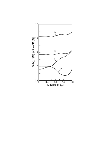
Figure 7: Kinetic energy loss function $D(M)$ in comparison to the Stoner parameter $I(M)$, obtained correctly (I), without inclusions of spin correlations $I_{2}$, and without any correlation corrections for the $J$-contributions, $I_{3}$ (from ref. soh ).

function $I_{corr}(m)$ (called $I(m)$ in the figure) in comparison to $D(m)$. As can be seen, it increases sizably with $m$. The origin is due to spin correlations. When these are turned off in the correlation calculation, the resulting quantity $I_{2}(m)$ no longer displays $m$-dependencies. Spin correlations are most relevant in the non-magnetic state and die out in the full magnetic limit. Also contained in the figure is the quantity $I_{3}(m)$ which is obtained when all interaction contributions originating from $J$ are treated in the $HF$-approximation.

This proper treatment of Hund’s rule effects, which corrects the Stoner parameter, strongly contrasts to fictitious disordered local moments that result from a locally symmetry broken HF-treatment of the exchange interaction. If such local moments existed in reality, then they would from the beginning prefer to order and to enhance the kinetic energy of the electrons.

The effect seen here is a quasi ’anti-disordered’ local moment effect. It definitely squeezes $Co$ into a first order magnetic phase transition. The non-magnetic ground state for $Co$ is even metastable at $T=0$. It requires a polarization beyond a critical size to destabilize it towards the ground state. Consequently, we would expect that the LSDA value for the transition temperature is not only overestimated due to a missing correlation correction of the kinetic energy loss, but that the true first order transition is considerably below that corrected quantity. We have not performed thermodynamic estimates but it looks as if the experimental $T_{c}$ for $Co$ might be reached this way. Our original choice of $U$ for $Co$ os had been motivated by the wish to bring $Co$ close to a second order phase transition.

Where $Ni$ is concerned, our results indicate a strong reduction of the magnetic energy in comparison to LSDA. For this case, a proper thermodynamic treatment has been made in DMFT li2 . The Hamiltonian was very close to the one that we used, and here also a local mean field or Stoner-theory was applied. The outcome was a $T_{c}$ slightly above the experimental value. Also the critical spin-fluctuations due to Stoner-enhancement just above $T_{c}$ were in good qualitative agreement with experiment. Corrections by spin-wave fluctuations that were disregarded in the DMFT calculations are definitely of relevance but have apparently little effect. One should remember, though, that the values of the interaction $U$ are not unambiguously fixed for the $Ni$-model calculations. The agreement of the DMFT calculations and experiment might originate in part from a value for $U$ that is slightly too small. On the other hand, there is again the trend that $I(m_{0})$ is 20 percent larger than $I(0)$soh , in part due to the spin correlations, and in part due to a small reduction of the change in $D(m)$. Since these two corrections are missing in LSDA-calculations, one would expect that the true Stoner-$T_{c}$ is considerably smaller than the LSDA-$T_{c}$.

For $Fe$, relative changes in the partial $n_{e_{g}}$ and $n_{t_{2g}}$ occupations with magnetization arise as artefacts of the five-band model. These cause an enhancement of $I_{SCF}(m)$ for small $m$. Being only partly screened by correlations, this partially compensates the corrections for small $m$ mentioned above. Nevertheless, a reduction of the magnetic energy by half was still found soh . However, this should, due to the pathology of the $Fe$-density of states, only lead to a reduction of $T_{c}$ by less than half gunn1 . The DMFT-calculation for a nine-band Hamiltonian for Fe produced in fact a $T_{c}$ of 2000K li2 , which is unsatisfactory. Here, the interactions were unambiguously fixed, and the deficiencies of the five-band model were absent.

Thus $Fe$ is the only case that still poses a major problem. There are two possible scenarios for its solution: either the phase transition in $Fe$ is not at all correctly described by a Stoner-like picture but rather by spin-wave fluctuation theories (for the earliest ones, see refs. 54 ; 55 ; 53 ), or, alternatively, the starting point, the rigid band system derived from LSDA together with local Hubbard-interactions is insufficient. Very recently, we obtained evidence sun that the latter case holds true. Its discussion is necessary for an understanding of the limits of a Hubbard model treatment but goes beyond the scope of this contribution. It will therefore be shortly addressed at the end.

V.4 Anisotropic Exchange Splitting for Ni

For ferromagnetic $Ni$, an interesting anisotropy occurs. The majority bands are completely filled. The charge in the minority bands is not equally distributed among the different $3d$-orbitals, but charge is missing almost exclusively from the $t_{2g}$-orbitals which form the most antibonding band states. This anisotropic charge distribution is, to a smaller amount, already present for the non-magnetic state without interaction (occupations of 0.98 or 0.92 for the $e_{g}$ and $t_{2g}$ orbitals, respectively). In the SCF-approximation, already for the non-magnetic state, an anisotropic crystal field exists. Even more interesting, for the ferromagnetic state, an anisotropic exchange splitting builds up. With exchange splitting, we refer to the difference in majority and minority crystal field terms. In the SCF-approximation, it holds for the splitting $\Delta_{SCF}(i)$ (with terms in the Hamiltonian $\Delta J$ disregarded)

$$\Delta_{SCF}(i)=(U+J)(n_{i\uparrow}-n_{i\downarrow})+Js_{z}$$ (41)

where

$$s_{z}=\sum_{i}(n_{i\uparrow}-n_{i\downarrow})\ \ .$$ (42)

While the second term is isotropic and amounts to 0.4eV for $Ni$, the first one contributes a splitting of 0.7eV only for the $t_{2g}$-orbitals.

With correlations, the interaction effects are partially screened. Also, a single-particle potential is no longer unambiguously defined. We obtained approximate values from our ground state calculations by keeping the correlation operators restricted to two-particle excitations, and by energy optimizing correlated states starting from different single determinant trial states that were each generated with particluar exchange splittings. The optimal trial state determined the ground state exchange splitting. We obtained for $Ni$ exchange splittings of $\Delta_{corr}(e_{g})=0.15eV$ and $\Delta_{corr}(t_{2g})=0.57eV$os . Actually, here interaction terms $\Delta J$ contributed. Without them, the splittings would be 0.27 and 0.50eV, respectively. These changes indicate a screening of the $J$ contributions by almost half, and of the $U$-contributions by more than half. Exchange splittings from LSDA come out isotropic and amount to 0.6eV.

These anisotropies were measured in angle resolved photoemission experiments him1 ; plu and came out as 0.1 or 0.4 eV, respectively. The agreement with our values is good; in particular if one takes into account that we computed our splitting for non-renormalized bands while in photoemission experiments the 15-20 percent mass renormalization due to many-body effects is included him ; cooke .

Many-body calculations for quasiparticle properties had actually been done before for a five-band Hamiltonian with very similar interactions (lacking the $\Delta J$ contributions). This calculation was based on the Kanamori t-matrix approximation, and had obtained splittings of 0.21 and 0.37 eV, with which our results agreed well. That computation had not only obtained the anisotropic splitting but also reasonable band renomalizations of 15 percent and even the experimentally seen shake up peak 58 ; 59 . Very recently, ground state calculations for a Hamiltonian similar to ours were performed, this time again within the $R=0$-approximation but for a 9-band model Hamiltonian, and by a full CI-calculation. The agreement for the exchange splitting was again very good (0.16 and 0.38 eV), but this time also relativistic contributions were included, and the experimental Fermi surface was reproduced with high quality web1 . Here, the anisotropic exchange splitting plays a big role, and the Fermi-surface of the LSDA is false.

In the computations, such anisotropies in the exchange splitting did not show up for $Co$, but we found them for $Fe$, too. In Fe, the $e_{g}$ orbitals carry a larger moment because the majority states are completely filled, but the minority bands are less populated than the $t_{2g}$ analogs. We had found splittings of $\Delta(e_{g})=1.74eV$ and $\Delta(t_{2g})=1.30eV$. LSDA-calculations obtain an isotropic splitting of 1.55eV, and experiments obtain 1.45eVhim but cannot resolve an anisotropy.

VI Interaction Parameters U

It is of interest to compare the interaction parameters $U$ obtained for $Fe$ to $Ni$ to parameters obtained by other means, and to try to gain a more global understanding. Fig. 8 contains these parameters as functions of the band filling.

Spectroscopy experiments for transition metal impurities in noble metals were interpreted with the help of atomic interactions saw . The values of the resulting quantity, $U$ (or $F_{0}$, as it is called in ref saw ), are given in Fig 8, too. They are in very good agreement with the $U$ obtained by the LA, in particular if one considers the different environments. This indicates that the screening patterns must be similar, and must also originate from the $4s,4p$-orbitals on the one hand, or from the $5s,5p$-orbitals on the other. In the impurity case, results exist for a whole range of transition metal impurities. The maximal reduction is obtained for the half-filled case (Cr) with $U=0.9$eV taken from spectroscopy results, while for less then half filling, the interaction increases again saw .

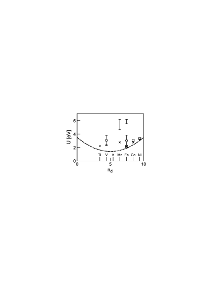
Figure 8: Values of the interaction $U$, obtained for different transition metals as a function of band filling. The values obtained by the LA are given as squares, the ones obtained from core spectroscopy saw are given by crosses. The full curve indicates the occupation dependence when a residual neighbor interaction $V$ is included. Bars with circles indicate estimates of $U$, obtained from ab-initio LA calculationssun , bars without circles estimates from frozen charge approximation computationscgunn ; gudra

The occupation dependence of $U$ can be understood with the help of a residual neighbor electron interaction $V$.

It has been worked out before for a single-band model s951 , how a Hamiltonian with on-site and neighbor interactions,

$$H_{int}=U_{0}\sum_{i}n_{\uparrow}(i)n_{\downarrow}(i)+{V\over 2}\sum_{(i,j)}a^{\dagger}_{\sigma}(i)a^{\dagger}_{\sigma^{\prime}}(j)a_{\sigma^{\prime}}(j)a_{\sigma}(i),$$ (43)

can be mapped into the Hubbard interaction $H_{int}=U\sum_{i}n_{\uparrow}(i)n_{\downarrow}(i)$. The sum over$(i,j)$runs over the $z$ nearest neighbors $j$ for each atom $i$. Here, it is implicitly assumed that all longer-range interactions are equal to zero. For the Hamiltonian with only on-site interactions, the only meaningfull response to the interaction can be condensed into the expectation value $\langle n_{\uparrow}(i)n_{\downarrow}(i)H_{int}\rangle$. It is therefore plausible to choose $U$ so that it yields the same response as the pair $U_{0},V$. Assuming for $\Psi_{0}$ the following relations for the single particle density matrix, $P(0)=<|n_{\sigma}(0)|>=n$, $P(0,l)=<|a^{\dagger}_{\sigma}(0)a_{\sigma}(l)|>\simeq p$ for ($l$)nearest neighbors, and zero elsewhere, one obtains

$$<|\overline{n_{i\uparrow}n_{i\downarrow}}H_{int}|>=U_{0}((n(1-n))^{2}+zp^{4})-2Vzn(1-n)p^{2}\ \ ,$$ (44)

and

$$U=U_{0}-{{2Vzn(1-n)p^{2}}\over{(n(1-n))^{2}+zp^{4}}}=U_{0}-\alpha V\ \ .$$ (45)

The parameter $U$ depends therefore on band filling as well as on the number of nearest neighbors. For almost empty bands, it holds that $p\simeq n$ since $k_{F}\ll{1\over{|\vec{R}_{i}-\vec{R}_{j}|}}$ and consequently $U\simeq U_{0}$. At half-filling, it follows from $P^{2}=P$, that $n\simeq n^{2}+zp^{2}$ and therefore $\alpha=2z/(z+1)$. For almost completely filled bands it holds that $\alpha\sim\delta n$, where $\delta n$ represents the number of holes. The curve drawn into Fig 8 is based on an $U_{0}=3.5eV$ and a $V=1.2eV$. It is deliberately put 0.5-1.0eV below the data points. Apparently, a pair of interactions $U=4.2eV,V=1.2eV$ can replace the so far independent terms for the specific elements.

Accepting such a residual interaction $V$ for the transition metals resolves a further problem. The LDA band width for transition metals is known to roughly agree with experiment for $Fe$ but to be too large for $Co$ and $Ni$ cooke ; him . The latter deficiency has been understood to arise from correlations caused by the on-site interactions 58 . From model calculations with the LA os ; soh , it can be deduced that the reduction of the band width $\delta W$ due to $U$ is similar in all three (!) cases. The apparent discrepancy for the case of $Fe$ can be resolved when a neighbor interaction $V=1.2$eV is included. The exchange broadening $\delta W$ due to $V$ increases the band width of Fe by 10% which partly compensates the correlation correction due to $U$. The exchange corrections for $Co$ and $Ni$ are smaller since it holds again that $\delta W\sim V\delta n$.

Effective local interactions $U$ were computed from LDA frozen charge calculations for the transition metal $Fe$ and for $Mn$ impurities in $Ag$ cgunn ; gudra . They are plotted in Fig. 8 as well. Apparently, these results do not depend on band filling. They are of the same size as for the case of $Cu$ with a completely filled 3d band cgunn . There, they match experiment. These frozen charge calculations actually computed the interaction costs to bring two electrons together from infinite distance but not the change in interaction from a neighbor site to the same site which is the relevant quantity in a half-filled band system. It is thus not astonishing that frozen charge LDA calculations are unable to treat band filling effects on effective local interactions.

The convolution of a longer range interaction into an on-site term alone is not sufficient to determine a model $U$. A model always lacks degrees of freedom that are present in the ab-initio calculation. If degrees of freedom were removed, then there is an alternative procedure to obtain a residual local interaction $U$. It is to require that particular correlation properties of the model are identical to the same ab-initio quantities. Due to the restriction of the model interaction to atomic terms, the relevant properties are atomic correlations. For the cases discussed here, the proper representative is the change of the atomic charge fluctuations $\Delta n^{2}$. For the model, this quantity was discussed in section IV.2. Exactly the same quantity can be calculated from ab-initio calculations. There, atomic orbitals are unambiguously defined, the same operators are included into the correlation calculations, and the same correlation function is available. $U$ is then chosen so that the model correlation function matches the ab-initio result. First applications have been presented in ref. s951 . From first ab-initio calculations, correlation functions for $V$ and $Fe$ are available sun . They lead to values of $U$ that are also included in Fig. 8. The big error bars originate from a mismatch of the five-band Hamiltonian to the correct atomic orbitals. We did not want to enter poorly described $3d$-orbitals with $4s$- and $4p$-tails into the ab-initio calculations. On the other hand, lacking a general tight-binding program, we could not improve the model. Also, in our ab-initio calculation, we did not treat the very short-range part of the correlation hole well. Thus, our ab-initio results rather represent an upper limit to the $U$.

Even for these error bars, the results show that an unambiguous convolution and condensation of the full Coulomb interaction into meaningful model interactions is possible. So far, model interactions were always chosen to fit a model to experiment. We had done so for the transition metals, and had obtained good agreement, but we had encountered other cases where a particular physical effect was incorrectly connected solely to an on-site interaction, and the resulting fit led to a wrong $U$. The case we have in mind is polyacetylene whose bond alternations also depends on interactions but not soleley on a local term $U$ ks ; s951 .

Of interest is also the case of the high $T_{c}$-superconducting compounds where we had performed such an analysis s98 ; st02 .

VII Relation of the Hubbard Model Results to the LSDA

In the previous chapters, we had shown how difficult an adequate treatment even of model interactions is. This makes it even more astonishing that LSDA-calculations managed to get sizable parts of magnetism correct, in particular the magnetic moments of the transition metals. To a certain degree this results from the fact that the $3d$-electrons are not too strongly correlated, and that for the delocalized electrons extended-Hückel features prevail, which the LSDA describes well. This may explain the cases of $Co$ and $Ni$, where the magnetic moment is maximal, provided the $3d$-band occupation is correct.

But as our evaluations have made clear, the correct magnitude of the magnetic moment of $Fe$ required an accuracy that the LSDA cannot possess. Consequently, the correct result can only arise due to a chance compensation of a set of errors. As was shown, the magnetic moment is determined by the Stoner-Parameter I, which depends equally on the local interactions $U$ and $J$ for five-fold degenerate systems.

Let us first sum up all contributions where $U$ alone is relevant, and connect these to LSDA deficiencies. $U$ dominates the strength of correlations. Due to $U$, electrons loose considerably more kinetic or band energy than would be expected for a homogeneous electron gas approximation. This can be seen in the Compton scattering. From the latter, one gets the impression that a treatment based on homogeneous electron gas ideas must miss most of $U$.

The next topic are binding energies, equilibrum distances and magneto-volume effect. All transition metals have LSDA binding energies that are too large - actually almost exactly by the amount which is removed by the residual $U$. Also the equilibrium distances are too short. The LSDA magneto-volume effect is always too large - in part, it can be corrected by effects of the residual $U$ soh ; kai .

Finally, the interaction $U$ causes sensitivities to charge anisotropies. This is relevant for the anisotropic exchange splitting of $Ni$. Due to its effect on the Fermi surface, it is basically a ground state property. LSDA lacks this splitting.

Consequently one may safely conclude that LSDA misses all $U$-contributions, or more cautiously expressed, it reduces $U$ to $J$ (this would avoid attractive interactions). This finding, however raises a problem. $U$ is very important for the Stoner parameter and for the magnetic moment. Roughly half of the weight in the latter comes from $U$. Consequently, a second error in connection with $J$ must occur.

$J$ leaves a direct imprint only on a single feature, namely the $m$ dependence of $I(m)$. Due to the inclusion of spin correlations, $I(0)$ is typically reduced by 10-20 percent in comparison to $I(m)$. Sadly, other contributions (in particular correlation effects due to $U$) cause a magnetic moment dependence, too. There is a single exception: $Co$. LSDA shows no feature like this, but on the other hand, there is not yet experimental evidence for this effect.

It is worth to investigate somewhat more how $I_{LSDA}$ is obtained from LSDA calculations. As mentioned before, whenever an LSDA calculation is made, even for atoms, $I_{LSDA}$ has the same value. In the atomic case, LSDA is assumed to describe the Hund’s rule ground state, and LDA is usually assumed to describe an average over all possible atomic states. Consequently, $I_{LSDA}$ must describe just the atomic exchange $J$, and it must do so in a mean-field approximation - this implies that no correction is possible without broken symmetry. In this respect it must behave exactly like a HF-theory, or like the incorrect SCF-approximation of our model Hamiltonian.

Only if LSDA behaves this way, can one understand why it obtains the correct moment for $Fe$ soh ; soh1 . $I$ depends roughly to equal parts on $U$ and $J$. Correlations reduce the effects of these terms by 40 percent from the SCF limit. As a consequence, the error involved in skipping $U$ (or in reducing it to $J$), is almost exactly compensated by the error in not correlating $J$. For magnetism in general, this compensation works only for 5-fold degeneracy. The error on the $U$-side is considerably larger than the error on the $J$-side for a single-band system. Consequently the LSDA must and usually does underestimate magnetism in general.

This latter deficiency is actually known, as the popularity of more recent ’$LDA$ plus $U$’-approximations demonstrates. Here, a local interaction is added to boost magnetism. However, all attempts to generate a kind of compensation within the DF-framework to upkeep the correct magnetic moment of $Fe$ have failed. They had to fail because the second error, the one for $J$ is of a different origin and thus independent. Even worse, these two are not the only LSDA-errors in the transition metal context as will be demonstrated in the next section.

These findings also call a particular field of LSDA-applications into question, namely all so called ab-initio disordered local moment calculations with which one has attempted to correct the false LSDA Stoner-theory results. As just derived, these LSDA disordered local moments are nothing but the false and inadequate model disordered local moment approximations for the Hubbard model. The local degrees of freedom generated by either method are artefacts of the approximation and have no connection to reality.

The only meaningful extensions of LDA-schemes are like the ones we had made for the first time a quarter century ago st ; os and like those that are now made in connection with DMFT-applications li2 : to condense the LDA results into a tight-binding Hamiltonian, to connect it to a local model interaction and to perform a careful correlation treatment of the latter.

A problem arises with the charge distributions in the ground state of these models. It is often, but not always, a good choice to freeze the charge distribution of this state to the one of the LDA-input. Counter-examples are the changes in the Fermi surface of $Ni$ that would not show up this way, or the inverse magneto-volume effect of $Ni$ that arises from anisotropic exchange contributions that cause a charge transfer from the $4s,4p$ to the $3d$-orbitals. There are also systems like the high $T_{c}$-superconductors where the LDA-charge distribution is wrong s98 ; st02 . As will be shown next, the case of $Fe$ is another example where it does not pay to stay close to LSDA-results even for the charge distribution.

VIII Ab-initio Correlation Calculations for $Fe$

As mentioned before, the model calculations using the LA are only a special application of the original ab-initio scheme. Here, first results of an ab-initio calculation for non-magnetic $Fe$ will be presented in order to contribute to the resolution of the open problem of $T_{c}$. We adress non-magnetic Fe, because we assume that the ferromagnetic state is rather well reproduced in LSDA. The moment is correct, and also the Fermi surface seems to be in agreement with experiment. The deficiences in the description of the magnetic phase transition might instead be connected to the non-magnetic ground state.

Like the non-magnetic HF-ground state and the LDA-ground state, the correlated non-magnetic ground state is theoretically well-defined. The only possible problem in the latter case might be that the added correlations allow long-range ferromagnetic patterns, and that in the approximation used the calculations turn instable. We proceeded only up to second nearest neighbor corrections for the case of $Fe$, and found no instability up to this range.

The details of the calculation will be given elsewhere sun . It should just be mentioned that for the HF- calculation and the parallel LDA-calculation the program Crystal was used crys . The basis set quality was of double-zeta quality, and better for the $3d$-electrons, and the computation was performed at the experimental lattice constant. A first correlation calculation starting from the LDA-ground state single determinant worked fine. Although the calculation was performed with the full and unscreened interaction, the electrons in the 9 valence orbitals screened each other perfectly. Correlations were as weak as for the model calculation with screened interaction. Note that this time for the 9 fluctuating channels, 45 correlation channels were available.

From the $3d$-correlation patterns we could also obtain an estimate on the effective local interactions, as mentioned before. This turned out to be $3\pm 1$eV, and was in reasonable agreement with the interaction needed for the Hubbard model treatment.

The LDA-charge distribution was analysed using the LA. Within this scheme, precise atomic orbitals are required for correlation purposes. A method had been developed to unambiguously obtain these from the single-particle density matrix $P_{ij}(l,l^{\prime})$ gps . For a similar application, see refs. s98 ; st02 .

Orbital	HF	LA	LDA	LDA(tbf)
$4s$	0.272	0.273	0.288	0.29
$4p$	0.203	0.173	0.163	0.06
$3d(t_{2g})$	0.966	0.715	0.678	0.73
$3d(e_{g})$	0.100	0.542	0.611	0.66
$\Delta$	0.866	0.173	0.067	0.07

Table 3: Charge distributions for bcc non magnetic $Fe$. Given are values for the HF, LA, and LDA calculations. Also values of a LDA tight binding fit papa are included.

The two right columns of table 3 contain our charge analysis in comparison to a standard tight-binding fit papa . There is good agreement, except a small charge transfer from the $4p$-orbitals into the $3d$-orbitals in the case of the fit. We assume that this occurs because for the fit, the completely empty $4p$-bands needed to be included which probably hybridize with the $4d$-bands. This apparently has an effect on the resulting charge distribution. In our numerical determination, only the occupied part of the bands was of relevance. The occupation anisotropy $\Delta=n_{t_{2g}}-n_{e_{g}}$ which is most relevant comes out the same.

When performing the HF-calculation, a very different charge distribution was obtained. The $4s$- and $4p$-orbital occupations did not change but a complete charge re-arrangement occured for the $3d$-orbitals. The $t_{2g}$-orbitals were almost completely filled, and the $e_{g}$-orbitals almost empty. This charge distribution is definitely incorect. It would never deliver the required sizeable binding energy contributions of the $3d$-bands. The values for the true ground state are also given. In particular $\Delta$ is considerably closer to the LDA-values.

This charge transfer represented by $\Delta$ is originally not connected to on-site interactions. Neither did our correlation calculation based on the LDA-ground state show instabilities toward a charge transfer, nor had the earlier model calculations given any hint for such a behaviour.

Rather, this charge transfer is due to a quantity that has been almost completely disregarded in the past: the non-local exchange. The long-range exchange contributions per site are formally of the form

$$\Delta E_{exch}=-\sum_{ijl}V(i,0;j,l)P_{ij}(0,l)^{2}.$$ (46)

Here, V is the Coulomb interaction term between orbital $i$ on site 0 and orbital $j$ on site $l$, and $P_{ij}(0,l)$ the corresponding density matrix that was introduced above. For the density matrix of a single-determinant state, the following sum rule applies

$$\sum_{jl}P_{ij}(0,l)^{2}=n_{i}.$$ (47)

As a consequence, delocalization pushes weight from neighbor terms into longer-range terms and costs considerable exchange energy. The amount is related to the size of long-range fluctuations and depends strongly on the density of states $n(E_{F})$. The latter, and even more the peak structure around it is very large for non-magnetic $Fe$, and is extremely costly in exchange energy. The peak structure is formed by antibinding $e_{g}$- and $t_{2g}$-orbitals. For the only non-local contribution to the LDA-calculation, the kinetic energy, this peak is apparently irrelevant, but adding only a small part of the non-local exchange immediately starts to separate the different contributions. The $e_{g}$-orbitals are pushed up, and the $t_{2g}$-orbitals are pushed down. When computed using the LDA, then the big charge transfer towards the LA-ground state costs less than 0.1eV per atom in energy. This is negligibly small in comparison to the binding energy and still smaller than the magnetization energy. However, 1.5eV are gained from the full exchange, and 0.3eV remain when the latter is screened. The ground state charge distribution is then further influenced by the strong spin correlations between the $e_{g}$-electrons forming when these reach half-filling.

The most relevant quantity in our context is the resulting density of states. The LDA- total density of states (summed over spins) and the one of the LA-ground state are given in Fig. 9. As can be seen, the LDA-peak close to the Fermi energy splits and is shifted to both sides of it.

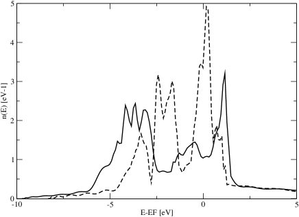
Figure 9: Total density of states $n(E)$ for bcc nonmagnetic$Fe$, obtained in LDA (dotted line) and by the LA (full line). $E_{F}$ is set to zero for both cases.

$n(e_{F})$ is reduced from $3.2eV^{-1}$ to $1.1eV^{-1}$. It becomes so small that the Stoner criterion is no longer fulfilled. Consequently, there is a true metastable non-magnetic bcc ground state for Fe, and the magnetic phase transition is of first order. Thus it is no wonder that there has been no chance to obtain a reasonable transition temperature starting from the unphysical non-magnetic ground state of the LDA. The instability of the LDA-state is such that already an admixture of only 5 percent of non-local exchange is sufficient to reduce the density of state at the Fermi energy by half.

These non-local exchange effects create a general trend towards weak localization. In $Fe$, they can act without symmetry breaking, but for single-band systems they would enter mostly via a symmetry-lowering charge-density-wave instability.

The LA-density of state indicates a widening of the $3d$-bands by 1.0eV. It has been obtained from a single-particle calculation with such a fraction of the non-local exchange added that the correct charge distribution was reproduced. Neither this density of state nor the original LDA-density of state contain any mass enhancements due to further many-body contributions. The latter should amount to 15-20 percent and shrink the band widths accordingly.

Sadly, no experimental informations about the density of states above the magnetic transition temperature are available. They might immediately verify our results since these differ strongly from LDA, and also from the ferromagnetic result, obtained either experimentally or in LSDA. There is no strong peak just below the Fermi-energy either, as it originates from the majority states in the ferromagnetic case.

There is an experiment, though, that can be explained by these new results: the measurements of the unoccupied Fe energy bands kir .

For this purpose, the energy bands of the LDA and of the LA ground state are presented in Fig. 10.

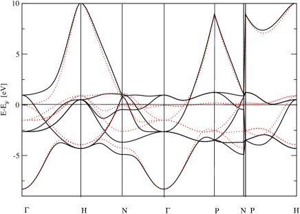
Figure 10: Energy bands of non magnetic bcc Fe from the LDA calculation (dots) and from the LA calculation (full lines). The occupied band width of the latter bands is renomalized to the one of the LDA bands.

The full lines represent the LA case, and the dotted bands the LDA case. This time, the LA bands have been renormalized so that the occupied width matches the LDA case, in order to facilitate comparison. The renormalization factor is 0.8, and may be deduced from Fig 9. As can be seen, non-local exchange has pushed the bands with $e_{g}$-character around $E_{F}$ roughly 1 eV above $E_{F}$, while bands with $t_{2g}$-character are a little lowered (around the H and N points). This explains the changes in the density of states.

It is of interest to compare the energy bands of the true non magnetic state with the ones of the ferromagnetic ground state. The latter can be derived from the LDA bands by either an upward shift by 1 eV for the minority bands or a downward shift by the same amount for the majority bands. As a consequence, the unoccupied minority bands are almost exactly where the corresponding non-magnetic bands are. An exception is the H point where minority and majority bands enclose the non-magnetic band asymmetrically.

With temperature increasing toward $T_{c}$, the unoccupied minority bands are therefore expected to stay in place while the bands around the H points are shifted. This is exactly what has been measured. The unoccupied minority and majority bands around the H point are shifted towards a center position, the former slightly more. The minority bands measured in the vicinity of the P point and in-between N and P points did not shift at all, however kir . These experiments fully comfirm our results for the non-magnetic ground state.

So far, the experimental results have been interpreted differently. It has been speculated that parts of the magnetic order do not break down when $T_{c}$ is reached, and that certain directions in momentum space might keep a magnetic memory for some unknown reasons. It would be worthwhile to re-analyse the experimental data and also to extract how the majority bands become emptied and jump towards the true non-magnetic bands.

The proper computation of the first order phase transition remains a topic to be addressed in the future. On the model level, this would imply to include at least neighbor interactions, and is definitely out of the range for the present DMFT. Further speculations on giant spin fluctuation theories should be put on hold, however, because it is very probable that they will never be needed for $Fe$, either.

We do not expect that non-local exchange contributions play a role for the ferromagnetic ground state of $Fe$, except for a certain band widening as has been discussed above (this is also why we have rescaled the LA bands to the LDA bands in Fig. 10). $n(E_{F})$ is already rather low for the ferromagnetic case. The role of non-local exchange contributions shrinks further when dealing with more strongly occupied bands as for $Co$ and $Ni$. Also, there is no peak in the density of states at the Fermi energy in these systems that might be removed.

On the other hand, we expect that these non-local exchange contributions play a significant role for the $Fe$-compounds. It is known that the LSDA usually does not treat these correctly, but it does so without an apparent systematic trend. The $Fe-O$-compounds come out more magnetic in reality than using the LSDA, while for the $Fe-Al$-compounds the inverse holds true. In all these cases, there is a sizable crystal field that $Fe$ itself lacks. This would make these compounds even more susceptible to a charge redistribution and accompanying weak localization than $Fe$ itself.

There is not only a competition between non-magnetic and magnetic states for the transition metals, but also one between more or less weakly localized states. While the interactions behind the former competition are $U$ and $J$, the ones behind the latter are $V$.

IX Conclusion

The aim of this work has been to present theoretical achievements in the computation of multi-band Hubbard models for transition metals. Luckily, this application turned out to be sufficiently remote from any kind of Mott-Hubbard transition so that currently well-controlled weak-correlation expansions could be used. As a consequence we can be certain that a model and not a deficiency in the treatment is responsible if we do not match experiment. We could exclude a strong-correlation scenario for a set of experimental findings, but the strongest argument against this scenario is the not fully magnetized ground state of $Fe$.

This weak-correlation scenario also made it possible to connect with LSDA-calculations, and to analyse and explain a set of errors, even failures, of the latter method.

Our findings indicate the seeming success of LSDA for the magnetism of the transition metals is basically due to a chance compensation of two big errors: an overscreening of $U$ on the one hand, and a mishandling of the atomic exchange interaction $J$ in a mean-field approximation on the other.

We have shown that these model interactions are of very similar size when obtained from fits to different experiments, and that it is even possible to understand the trend among these values for different transition metals. This indicates that these model interactions are more meaningful quantities than just fitting parameters. We have also given an indication of how these parameters will, in the future, be directly computed from ab-initio correlation calculations using the LA.

On the model level, a set of different properties could be understood. Also with the help of more extensive CI-calculations web1 , and in particular thanks to quasiparticle calculations using the DMFT li2 , a basic understanding has finally been reached of the problems that had been raised half a century ago sto ; vv ; wo ; 33 ; he , and that had been mostly put aside the last forty years as far as the DF-approach has been concerned.

We now know that the magnetic phase transition of the transition metals can basically be described following the ideas of Stoner and Wohlfarth, and that the electrons stay almost completely delocalized. We also know that orbital degeneracy plays the most important role in this context, and that the atomic exchange interaction is of great importance.

A very surprising twist is that for the magnetism of $Fe$, also residual non-local interactions seem to be relevant. There has been earlier evidence that they are present in $Fe$, originating from trends in the dependence of $U$ on the individual atoms, and from matches and mismatches of theoretical and experimental photoemission results. These non-local interaction contributions lead to big changes of the LDA-results for the non-magnetic ground state, although those latter results were and still are the basis of a satisfying description of the ferromagnetic ground state.

All these findings demonstrate how important it is to understand and to treat the interactions of the electrons directly. It is an advantage of the LA that the correlation treatment does not disappear within the black box of a numerical program but that all different correlation details can be directly obtained and understood. One aim of this contribution was to present, with the help of the LA, a lucid and understandable decomposition of the complex many-body world.

References

- (1) P. Hohenberg and W. Kohn, Inhomogeneous electron gas, Phys. Rev. 136, 864 (1964).
- (2) W. Kohn and L.J. Sham, Self consistent equations including exchange and correlation effects, Phys. Rev. 140, 1133 (1965).
- (3) O. Gunnarsson and B.I. Lundqvist, Exchange and correlation in atoms, molecules, and solids by the spin-density-functional formalism, Phys.Rev.B13, 4274 (1976).
- (4) U.K. Poulson, J. Kollar, and O.K. Anderson, Magnetic and cohesive properties from canonical bands, J. Phys. F6, L 241 (1976).
- (5) J. F. Janak and A. R. Williams, Giant internal magnetic pressure and compressibility anomalies, Phys. Rev. B14, 4199 (1976).
- (6) J. Callaway in Physics of Transition Metals (Inst. of Physics, Bristol, 1981).
- (7) J. Friedel in The Physics of Metals (Cambridge U. Press, Cambridge, 1969).
- (8) V. L. Moruzzi, J. F. Janak, and A. R. Williams, Calculated Electronic Properties of Metals (Pergamon, New York, 1978).
- (9) G. Stollhoff and P. Fulde, On the computation of electronic correlation energies within the local approach, J. Chem. Phys. 73(9), 4548 (1980).
- (10) G. Stollhoff, The local ansatz extended, J. Chem. Phys. 105, 227 (1996).
- (11) A. Heilingbrunner and G. Stollhoff, Ab-initio correlation calculation for metallic lithium, J. Chem. Phys. 99, 6799 (1993).
- (12) G. Stollhoff, Electrons in high- compounds: ab-initio correlation results, Phys. Rev. B 58, 9826 (1998).
- (13) G. Stollhoff, unpublished.
- (14) L. Kleinmann and K. Mednick, Self-energy contributions to the electronic structure of Ni, Phys. Rev. B24, 6880 (1981).
- (15) T. Moriya (ed.), Electron Correlation and Magnetism in Narrow Band systems, Springer Ser. Solid-State Sci., Vol 29 (Springer, Berlin 1981).
- (16) G. Stollhoff and P. Thalmeier, Variational Treatment of Electronic Correlations in -Band Metals, Z.Physik B 43, 13 (1981).
- (17) A. M. Oleś and G. Stollhoff, Correlation effects in ferromagnetism transition metals, Phys. Rev. B 29, 314 (1984).
- (18) E. C. Stoner, Proc. R. Soc. London, Collective electron Ferromagnetism Ser. A 165, 372 (1938).
- (19) E. P. Wohlfarth, Proc. R. Soc. London, Collective electron Ferromagnetism III Nickel and nickel-copper alloys, Ser. A 195, 434 (1949).
- (20) O. Gunnarsson, Band model for magnetism of transition metals in the spin-density-functional formalism, J. Phys. F 6, 587 (1976).
- (21) A. M. Oles, G. Stollhoff, Correlation Corrections for the Stoner Parameter of Ferromagnetic Transition Metals, Europhys. Lett. 5, 175 (1988).
- (22) G. Stollhoff, A. M. Oleś, and V. Heine, Stoner exchange interaction in transition metals, Phys. Rev. B 41, 7028 (1990).
- (23) G. Stollhoff, A. M. Oleś, and V. Heine, Comment on Relationship between the Coulomb Integral and the Stoner Parameter , Phys. Rev. Lett. 76, 855 (1996).
- (24) T. Moriya, Spin fluctuations in Itinerant Electron Magnetism, Springer Ser. Solid-State Sci., Vol 56 (Springer, Berlin 1985).
- (25) F. Kajzar and J. Friedel, Role of the intraatomic Coulomb correlation on the energy of cohesion in narrow band metals, J. Physique 39, 397 (1978).
- (26) G. Treglia, F. Ducastelle, and D. Spanjaard, Perturbation treatment of correlations in transition metals, J. Physique 41, 281 (1980).
- (27) J. Kanamori, Electron correlation and ferromagnetism in transition metals, Progr. Theor. Phys. 30, 275 (1963).
- (28) A. Liebsch, Effect of self-energy on the valence-band photoemission spectra of Ni, Phys. Rev. Lett. 43, 1431 (1979).
- (29) A. Liebsch, Ni -band self-energy beyound the low-density limit, Phys. Rev. B23, 5203 (1981).
- (30) D. Penn, Effect of bound hole pairs on the -band photoemission spectrum of Ni, Phys. Rev. Lett.42, 921 (1979).
- (31) L. C. Davis and L. A. Feldkamp, Quasi-particle energies and two-hole xps satellite in Ni, Solid State Commun. 34, 141 (1980).
- (32) J. Bünemann, W. Weber, and F. Gebhard, Multiband Gutzwiller wave functions for general on-site interactions Phys. Rev. B 57, 6896 (1998).
- (33) J. Bünemann et al., Atomic correlations initinerant ferromagnets: Quasi-particle bands of Ni, Europhys. Lett. 61, 667 (2003).
- (34) A. Lichtenstein, M. I. Katsnelson, and G. Kotliar, Finite-temperature magnetism of transition metals: an ab initio dynamical mean-field theory, Phys. Rev. Lett. 87, 067205 (2001).
- (35) O. K. Andersen and O, Jepsen, Advances in the theory of one-electron energy states, Physica B 91, 317 (1977).
- (36) M. C. Gutzwiller, Corredlation of electrons in a narrow band Phys. Rev. 137, 1726 (1965).
- (37) R. Jastrow, Many-Body problem with strong forces, Phys. Rev 98, 1479 (1955).
- (38) F. Coester, Nucl. Phys. 7,421 (1958).
- (39) F. Coester and H. Kümmel, Nucl. Phys. 17, 477 (1960).
- (40) J. Cizek, On the correlation problem in Atomic and Molecular Physics J. Chem. Phys.45, 4256 (1966).
- (41) J. Cizek, Adv. Chem. Phys. 14, 35 (1969).
- (42) D. Vollhardt et al., Metallic ferromagnetism: progress in our understanding of an old strong-coupling problem, Advances in Solid State Physics, Vol.38, 383 (1999).
- (43) G. Stollhoff, and A. Heilingbrunner, Coupled-cluster equations for the local ansatz, Z. Physik B83,85 (1991).
- (44) P. Unger, J. Igarashi, and P. Fulde, Electronic excitations in transition metals, Phys. Rev. B50, 10485 (1994).
- (45) M. I. Katsnelson and A. I. Lichtenstein, LDA++approach to the electronic structure of magnets: correlation effects in Fe, J. Phys. Cond. Matter 11, 1037 (1999).
- (46) G. Stollhoff, Magnetic correlations in the paramagnetic state of -transition metals, J. Magn. Magn. Mat. 54-57, 1043 (1986).
- (47) P. J. Brown, D. Deportes,D. Givord, and K. R. A. Ziebeck, Paramagnetic scattering studies of the short-range order above in transition metals compounds and pure Fe, J. Appl. Phys. 53, 1973 (1982).
- (48) M. M. Steiner, R. C. Albers, and L. J. Sham, Quasiparticle properties of Fe, Co, and Ni, Phys. Rev. B 45, 13272 (1992).
- (49) V. Korenman, J. L. Murray, and R. E. Prange, Local band theory of itinerant ferromagnetism. I Fermi-liquid theory, Phys. Rev. B16, 4032 (1977)
- (50) H. Capellmann, Ferromagnetism and strong correlations in metals, J. Phys. F 4, 1466 (1974).
- (51) H. Capellmann, Theory of itinerant ferromagnetism in the -transition metals, Z. Physik B 34, 29 (1979).
- (52) G. E. Bauer and J. R. Schneider, Electron correlation effect in the momentum density of copper metal, Phys. Rev.B 31, 681 (1985).
- (53) A. J. Rollason, M. Cooper, and R. S. Holt, Directional Compton profiles and the electron density distribution in V, Philos. Mag.B 47, 51 (1983).
- (54) S. Wakoh and M. Matsumoto, Correlation correction on Compton profiles of V and Cr, J. Phys. Cond. Matter 2, 797 (1990).
- (55) D. L. Anastassopoulos, G. D. Priftis, N. I. Papanicolaou, N. C. Bacalis, and D. A. Papaconstantopoulos, Calculation of the electron moment density and Compton scattering measurements for Ni, J. Phys. Cond. Matter 3, 1099 (1991).
- (56) A. J. Rollason, R. S. Holt, and M. J. Cooper, Directional Compton profiles and the electron density distribution in Fe, J. Phys. F 13, 1807 (1983).
- (57) V. Sundararajan, D. G. Kanhere, and R. M. Singru, Calculation of spin-dependent momentum distributions in Fe: Ccompton scattering and positron annihilation, J. Phys. Cond.Matter 3, 1113 (1991).
- (58) G. Stollhoff, Compton scattering and Electron Correlations in the Transition Metals, Europhys. Lett. 29, 463 (1995).
- (59) D. E. Eastman, F. J. Himpsel, and J. A. Knapp, Experimental band structure and temperature-dependent magnetic exchange splitting of Ni using angle-resolved photoemission Phys. Rev. Lett. 40, 1514 (1978).
- (60) W. Eberhardt and E. W. Plummer, Angle-resolved photoemiision determination of the band structure and multielectron excitations in Ni, Phys. Rev. B 21, 3245 (1980).
- (61) D. E. Eastman, F. J. Himpsel, and J. A. Knapp, Experimental Exchange-split energy-band dispersions for Fe, Co, Ni, Phys. Rev. Lett. 44, 95 (1980).
- (62) J. F. Cooke, J. W. Lynn, and H. L. Davis, Calculations of the dynamic susceptibility of Ni and Fe, Phys. Rev. B 21, 4118 (1980).
- (63) D. van der Marel and G. A. Sawatzky, Electron-elecron interaction and localization in and transition metals, Phys. Rev. B 37, 10674 (1988).
- (64) G. Stollhoff, From ab-initio Calculations to the Hubbard Model and beyound, Europhys. Lett. 30, 99 (1995).
- (65) V. I. Anisimov and O. Gunnarsson, Density -functional calculation of effectrive Coulomb interactions in metals, Phys. Rev. B 43, 7570 (1991).
- (66) V. Drchal, O. Gunnarsson and O. Jepsen, Effrective Coulomb interaction in metallic -systems: comparison of theory and experiment for Mn in Ag Phys. Rev. B 44, 3518 (1991).
- (67) G. König and G. Stollhoff, Why polyacetylene dimerizes: results of ab initio computations, Phys. Rev. Lett. 65, 1239 (1990).
- (68) G. Stollhoff, Electron correlations in the high- compounds, Cimtec 2002 Proc. Forum on New Materials Vol.3, pp229 (2002).
- (69) A. B. Kaiser, A. M. Oles, and G. Stollhoff, Volume dependence of the Stoner Parameter in Transition Metals, Phys. Scr. 37, 935 (1988).
- (70) V.R. Saunders et al., Crystal98 User’s Manual, University of Torino (1998).
- (71) R. Pardon, J. Gräfenstein, and G. Stollhoff, Ab initio ground-state correlation calculations for semiconductors with the local ansatz, Phys. Rev. B51, 10556 (1995).
- (72) D. A. Papaconstantopoulos, The band structure of Elemental solids (Plenmu, New York,1968).
- (73) J. Kirschner, M. Gloebl, V. Dose, and H. Scheidt, Wave-vector-dependent temperature behaviour of empty bands in ferromagnetic Iron, Phys. Rev. Lett 53, 612 (1984).
- (74) J. H. van Vleck, Rev. Mod. Phys. 17, 27 (1945).
- (75) C. Herring, in Magnetism (Eds. G. Rado, H. Suhl) Vol. 4 (Academic Press,1966).