Abstract

We construct a holographic dark energy model with a non-minimally coupled scalar field on the brane where Gauss-Bonnet and Induced Gravity effects are taken into account. This model provides a wide parameter space with several interesting cosmological implications. Especially, the equation of state parameter of the model crosses the phantom divide line and it is possible to realize bouncing solutions in this setup.
PACS: 04.50.-h,  98.80.-k, 95.36.+x
Key Words: Dark Energy, Scalar-Tensor Theories, Induced Gravity, Stringy Effects, Cosmological dynamics

1 Introduction

Recent observational data from CMB temperature fluctuations spectrum, Supernova type Ia redshift-distance surveys and other data sources, have shown that the universe is currently in a positively accelerated phase of expansion and its spatial geometry is nearly flat  [1]. Reconciling to Einstein’s field equations, $G_{\mu\nu}=8\pi GT_{\mu\nu}$, we see that to explain these important achievements, we need either to modify the matter part of the theory by incorporating an additional cosmological component as dark energy ( that is, $G_{\mu\nu}=8\pi G[T^{(M)}_{\mu\nu}+T^{(Dark)}_{\mu\nu}]$  where $T^{(M)}_{\mu\nu}$ and $T^{(Dark)}_{\mu\nu}$ are energy-momentum tensor of ordinary matter and dark energy component respectively) or modify the geometric part of the field equations as the manifestation of the ”dark geometry” ( that is, $G_{\mu\nu}+G^{(Dark)}_{\mu\nu}=8\pi GT^{(M)}_{\mu\nu}$ )[2]. Multi-component dark energy with at least one non-canonical phantom field is a possible candidate of the first alternative. This viewpoint has been studied extensively in literature [3]. Extension of the general relativity to more general theories on cosmological scales is the basis of the second alternative ( see for instance [4,5] ). The DGP ( Dvali-Gabadadze-Porrati) braneworld scenario as an infra-red (IR) modification of the general relativity, explains accelerated expansion of the universe in its self-accelerating branch via leakage of gravity to extra dimension [6]. In this model, the late-time acceleration of the universe is driven by the manifestation of the excruciatingly slow leakage of gravity off our four-dimensional braneworld into an extra dimension.

There are some datasets (such as the Gold dataset) that show a mild trend for crossing of the cosmological constat line by the equation of state (EoS) parameter of dark component in the first alternative. The equation of state parameter in these scenarios crosses the phantom divide ( $\omega=\frac{p}{\rho}=-1$) line at recent redshifts and current accelerated expansion requires $\omega<-\frac{1}{3}$. The current best fit value of the equation of state parameter, using WMAP five year data combined with measurements of type Ia supernovae and Baryon Acoustic Oscillations ( BAO ) in the galaxy distribution, is given by $-0.11<1+\omega<0.14$ ( with $95$ percent CL uncertainties) ( see the paper by Komatsu et al. in Ref. [1]). It is accepted that crossing of the phantom divide line occurs at recent epoch with $z\sim 0.25$ [3].

In the second alternative and within self-accelerating branch of the DGP scenario, the EoS parameter never crosses the $\omega(z)=-1$ line, and universe eventually turns out to be de Sitter phase. However, in this setup if we use a single scalar field (ordinary or phantom) on the brane ( in both branches of the scenario), we can show that EoS parameter of dark energy can cross the phantom divide line [7,8]. In a braneworld setup with induced gravity embedded in a bulk with arbitrary matter content, the transition from a period of domination of the matter energy density by non-relativistic brane matter to domination by the generalized dark radiation provides a crossing of the phantom divide line [9]. Quintessential scheme can also be achieved in a geometrical way in higher order theories of gravity [10]( see also [4]). Phantom-like behavior without phantom matter [8] and also phantom-like behavior in a brane-world setup with induced gravity and curvature effects have been reported [11].

In a braneworld scenario, the radiative corrections in the bulk lead to higher curvature terms on the brane. At high energies, the Einstein-Hilbert action will acquire quantum corrections. The Gauss-Bonnet (GB) combination arises as the leading bulk correction in the case of the heterotic string theory [12]. This term leads to second-order gravitational field equations linear in the second derivatives in the bulk metric which is ghost free [13-15], the property of curvature invariant of the Gauss-Bonnet term. Inclusion of the Gauss-Bonnet term in the action results in a variety of novel phenomena which certainly affects the cosmological consequences of these generalized braneworld setup, although these corrections are smaller than the usual Einstein-Hilbert terms [16-21]. We note that in a DGP+GB scenario which we call it GBIG, while induced gravity is a manifestation of the IR limit of the model, the Gauss-Bonnet term is essentially related to the UV limit of the scenario.

With these preliminaries, the purpose of this paper is to construct a holographic dark energy model in a DGP setup with induced gravity and Gauss-Bonnet effect. We consider a scalar field non-minimally coupled to induced gravity on the brane as a dark energy component in the presence of radiative corrections. We study a general case in which a DGP brane with non-vanishing tension is embedded in an AdS bulk and a scalar field non-minimally coupled to induced gravity is presented on the brane. We study dynamics of the equation of state parameter of holographic dark energy component in this setup. Due to a wide parameter space, this model accounts for crossing of the phantom divide line and it is possible to realize bouncing solutions in this framework ( for a review of bouncing solutions see [22]). A crucial point should be stressed here: the Gauss-Bonnent braneworld scenario with induced gravity essentially dose not need to introduce any scalar field to realize phantom divide line crossing. In other words, the combination of the effect of the Gauss-Bonnent term in the bulk and induced gravity term on the brane behaves itself as a dark energy on the brane [14]. However, incorporation of a scalar field non-minimally coupled to induced gravity on the brane leads to several interesting features such as shift of the initial conditions for finite big bang scenario and possibility to realize bouncing solutions [21]. As we will show, inclusion of this non-minimally coupled scalar field on the brane brings several new consequences in the spirit of the holographic dark energy model. So, due to apparent gap in the study of the holographic dark energy with induced gravity and Gauss-Bonnet term and also to have a complete picture of these types of scenarios, this paper considers a scalar field which is non-minimally coupled to the induced gravity in the presence of the Gauss-Bonnet term in the bulk. Finally, we study some especial cases by adopting suitable ansatz and also we address the issue of ghost instabilities in this setup.

2 A Non-Minimally Coupled Scalar field on the DGP Brane

The action of the DGP scenario in the presence of a non-minimally coupled scalar field on the brane can be written as follows [21]

$$S=\frac{1}{2\kappa_{5}^{2}}\int d^{5}x\sqrt{-g^{(5)}}\Big{[}R^{(5)}-2\Lambda_{5}\Big{]}$$

$$+\Bigg{[}\frac{r}{2\kappa_{5}^{2}}\int d^{4}x\sqrt{-g}\bigg{(}\alpha(\phi)R-2\kappa_{4}^{2}g^{\mu\nu}\nabla_{\mu}\phi\nabla_{\nu}\phi-4\kappa_{4}^{2}V(\phi)-4\kappa_{4}^{2}\lambda\bigg{)}\Bigg{]}_{y=0},$$ (1)

where we have included a general non-minimal coupling $\alpha(\phi)$ in the brane part of the action. $y$ is coordinate of the fifth dimension and we assume the brane is located at $y=0$.  $g^{(5)}_{AB}$ is five dimensional bulk metric with Ricci scalar ${R^{(5)}}$, while $g_{\mu\nu}$ is induced metric on the brane with induced Ricci scalar $R$.  $\lambda$ is the brane tension (constant energy density) and $r$ is the crossover scale that is defined as follows

$$r=\frac{\kappa_{5}^{2}}{2\kappa_{4}^{2}}=\frac{M_{4}^{2}}{2M_{5}^{3}}.$$ (2)

The generalized cosmological dynamics of this setup is given by the following Friedmann equation [19-21]

$$\varepsilon\sqrt{H^{2}-\frac{{\cal{M}}}{a^{4}}-\frac{\Lambda_{5}}{6}+\frac{K}{a^{2}}}=r\alpha(\phi)\Big{(}H^{2}+\frac{K}{a^{2}}\Big{)}-\frac{\kappa_{5}^{2}}{6}(\rho+\rho_{\phi}+\lambda)\,,$$ (3)

where $\varepsilon=\pm 1$ are corresponding to two possible branches of the DGP cosmology and ${\cal{M}}$ is the bulk black hole mass which is related to the bulk Weyl tensor. The DGP limit has a Minkowski bulk $\Lambda_{5}=0$ with ${\cal{M}}=0$. We note that braneworld model with scalar field minimally or non-minimally coupled to gravity have been studied extensively [23]. The introduction of non-minimal coupling (NMC) is forced upon us in many situations of physical and cosmological interests as addressed in Ref. [24]. Assuming the following line element

$$ds^{2}=q_{\mu\nu}dx^{\mu}dx^{\nu}+b^{2}(y,t)dy^{2}=-n^{2}(y,t)dt^{2}+a^{2}(y,t)\gamma_{ij}dx^{i}dx^{j}+b^{2}(y,t)dy^{2},$$ (4)

where $\gamma_{ij}$ is a maximally symmetric 3-dimensional metric defined as $\gamma_{ij}=\delta_{ij}+k\frac{x_{i}x_{j}}{1-kr^{2}}$, the energy density of the non-minimally coupled scalar field on the brane is given as follows [21,23]

$$\rho_{\phi}=\left[\frac{1}{2}\dot{\phi}^{2}+n^{2}V(\phi)-6\alpha^{\prime}H\dot{\phi}\right]_{y=0},$$ (5)

where  $H=\frac{\dot{a}}{a}$  is Hubble parameter on the brane,  $\alpha^{\prime}=\frac{d\alpha}{d\phi}$ and $\dot{\phi}=\frac{d\phi}{dt}$.

If we consider a flat ($k=0$) brane with $\lambda=0$ and also a Minkowski bulk ($\Lambda_{5}=0$, ${\cal{M}}=0$), then we can write equation (3) as follows

$$H^{2}=\pm\frac{H}{r\alpha(\phi)}+\frac{\kappa_{4}^{2}}{3\alpha(\phi)}\Big{(}\rho+\rho_{0\phi}-6\alpha^{\prime}H\dot{\phi}\Big{)},$$ (6)

where $\rho_{0\phi}=\left[\frac{1}{2}\dot{\phi}^{2}+n^{2}V(\phi)\right]_{y=0}$. The DGP model has two branches, i.e   $\varepsilon=\pm 1$ corresponding to two different embedding of the brane in the bulk. The behavior of two branches at high energies and low energies are summarized as follows:
In the high energy limit we find

$$\hskip 42.67912ptDGP(\pm):\,\,\,\,\,\,\,\,H^{2}=\frac{\kappa_{4}^{2}}{3\alpha(\phi)}(\rho+\rho_{\phi}),$$ (7)

while in the low energy limit we have

$$DGP(+):\,\,\,\,\,\,\,\,H\longrightarrow\frac{1}{r\alpha(\phi)}-2\frac{\kappa_{4}^{2}\alpha^{\prime}\dot{\phi}}{\alpha(\phi)}$$

$$DGP(-):\,\,\,\,\,\,\,\,H=0.$$ (8)

In terms of dimensionless variables introduced in [19,20]

$$h=Hr,\,\,\,\mu=\frac{r\kappa_{5}^{2}}{6}\rho,\,\,\,\,\bar{\mu}=\frac{r\kappa_{5}^{2}}{6}\rho_{0\phi},\,\,\,\,\sigma=\frac{r\kappa_{5}^{2}}{6}\lambda,\,\,\,\,\tau=\frac{t}{r},$$ (9)

we find

$$h^{2}=\pm\frac{h}{\alpha(\phi)}+\frac{(\mu+\bar{\mu})}{\alpha(\phi)}-\frac{2h\kappa_{4}^{2}}{\alpha(\phi)}\frac{d\alpha}{d\tau}.$$ (10)

The solutions of this equation for $h$ are as follows

$$h=\pm\frac{1}{2\alpha(\phi)}-\frac{\kappa_{4}^{2}}{\alpha(\phi)}\frac{d\alpha}{d\tau}+\frac{\sqrt{1\mp 4\kappa_{4}^{2}\frac{d\alpha}{d\tau}+4(\kappa_{4}^{2}\frac{d\alpha}{d\tau})^{2}+4\alpha(\phi)(\mu+\bar{\mu}+\sigma)}}{2\alpha(\phi)}.$$ (11)

Here the negative root is not suitable since in the limit of   $(\mu+\bar{\mu})\longrightarrow 0$, with this choice of sign one cannot recover the low energy limit of the model as given by (7).

As we have note, the DGP model is an IR modification of the general relativity. In the UV limit, stringy effects will play important role. In this viewpoint, to discuss both UV and IR limit of a cosmologically viable braneworld scenario simultaneously, the DGP model is not sufficient and we should incorporate stringy effects via inclusion of the Gauss-Bonnet term.

3 Incorporation of the Gauss-Bonnet Effect

The Gauss-Bonnet term with coupling constant $\beta$ is written as follows

$$L_{GB}=R^{(5)2}-4R_{ab}^{(5)}R^{(5)ab}+R_{abcd}^{(5)}R^{(5)abcd}$$

where $R^{(5)}$ is the curvature scalar of the 5-dimensional bulk spacetime. These corrections have origin on stringy effects and the most general action should involve both Gauss-Bonnet and the Einstein-Hilbert term in 5D theory. The action of the GBIG (Gauss-Bonnet (GB) term in the bulk and the Induced Gravity (IG) term on the brane) scenario in the presence of a non-minimally coupled scalar field on the brane can be written as follows [21]

$$S=\frac{1}{2\kappa_{5}^{2}}\int d^{5}x\sqrt{-g^{(5)}}\Bigg{[}R^{(5)}-2\Lambda_{5}+\beta\Big{(}R^{(5)2}-4R_{ab}^{(5)}R^{(5)ab}+R_{abcd}^{(5)}R^{(5)abcd}\Big{)}\Bigg{]}$$

$$+\Bigg{[}\frac{r}{2\kappa_{5}^{2}}\int d^{4}x\sqrt{-g}\bigg{(}\alpha(\phi)R-2\kappa_{4}^{2}g^{\mu\nu}\nabla_{\mu}\phi\nabla_{\nu}\phi-4\kappa_{4}^{2}V(\phi)-4\kappa_{4}^{2}\lambda\bigg{)}\Bigg{]}_{y=0},$$ (12)

where $\beta$ and $r$ are the GB coupling constant and IG cross-over scale respectively. The relation for energy conservation on the brane is as follows

$$\dot{\rho}+\dot{\rho}_{\phi}+3H(1+\omega)(\rho+\rho_{\phi})=6\alpha^{\prime}\dot{\phi}\Big{(}H^{2}+\frac{k}{a^{2}}\Big{)}.$$ (13)

where $\omega=\frac{p+p_{\phi}}{\rho+\rho_{\phi}}$  with $p$ and $\rho$ pressure and density of the ordinary matter on the brane. The cosmological dynamics of the model is given by the following generalized Friedmann equation

$$\Bigg{[}1+\frac{8}{3}\beta\Big{(}H^{2}+\frac{\Psi}{2}+\frac{K}{a^{2}}\Big{)}\Bigg{]}^{2}\Big{(}H^{2}-\Psi+\frac{K}{a^{2}}\Big{)}=\Bigg{[}r\alpha(\phi)H^{2}+r\alpha(\phi)\frac{K}{a^{2}}-\frac{\kappa_{5}^{2}}{6}(\rho+\rho_{\phi}+\lambda)\Bigg{]}^{2}.$$ (14)

This equation describes the cosmological evolution on the brane with tension and a non-minimally coupled scalar field on the brane. The bulk contains a black hole mass and a cosmological constant. $\Psi$ is defined as follows

$$\Psi+2\beta\Psi^{2}=\frac{\Lambda_{5}}{6}+\frac{{\cal{M}}}{a^{4}}.$$ (15)

If $\beta=0$, the model reduces to DGP model, while for $r=0$ we recover the Gauss-Bonnet model. Here we restrict our study to the case where bulk black hole mass vanishes, (${\cal{M}}=0$) and therefore $\Psi+2\beta\Psi^{2}=\frac{\Lambda_{5}}{6}$. The bulk cosmological constant in the presence of GB term is given by $\Lambda_{5}=-\frac{6}{l^{2}}+\frac{12\beta}{l^{4}}$, where $l$ is the bulk curvature. For a spatially flat brane ($k=0$), the Friedmann equation is given by

$$\Bigg{[}1+\frac{8}{3}\beta\Big{(}H^{2}+\frac{\Psi}{2}\Big{)}\Bigg{]}^{2}\Big{(}H^{2}-\Psi\Big{)}=\Bigg{[}r\alpha(\phi)H^{2}-\frac{\kappa_{5}^{2}}{6}(\rho+\rho_{\phi}+\lambda)\Bigg{]}^{2}.$$ (16)

We define the following dimensionless quantities

$$\gamma=\frac{8\beta}{3r^{2}},\hskip 28.45274pt\chi=\frac{r^{2}}{l^{2}},\hskip 28.45274pt\psi=\Psi r^{2},$$ (17)

where the dimensionless Friedmann equation takes the following form

$$\Bigg{[}1+\gamma\Big{(}h^{2}+\frac{\psi}{2}\Big{)}\Bigg{]}^{2}\Big{(}h^{2}-\psi\Big{)}=\Bigg{[}\alpha(\phi)h^{2}-\Big{(}\mu+\bar{\mu}+\sigma-2\frac{d\alpha(\phi)}{d\tau}h\kappa_{4}^{2}\Big{)}\Bigg{]}^{2}.$$ (18)

To find cosmological dynamics of our model, we should solve this equation in an appropriate parameter space. In which follows, we consider a general case with brane tension ($\sigma\neq 0$) and AdS bulk. Before proceeding further, we should stress on two important points here: firstly, the presence of GB term removes the big bang singularity in this setup, and the universe starts with an initial finite density [19,20]. Gauss-Bonnet effect is essentially a string-inspired effect in the bulk which its combination with pure DGP scenario leads to a finite big bang proposal on the brane. Secondly, non-minimal coupling of the scalar field and induced gravity on the brane controls the value of the initial density [21].

3.1 A Brane with Non-Vanishing Tension Embedded in an AdS Bulk

In the case with $\psi\neq 0$, the bulk is AdS since in this case $\Lambda_{5}\neq 0$. We should solve equation (18) for this case. The condition $h=0$ gives two solutions

$$\mu_{b,c}=\mp\sqrt{-\psi}(1+\frac{\psi}{2})-\sigma,$$ (19)

where $\mu_{c}$ is the density at the point that the solution corresponding to plus sign collapses, while $\mu_{b}$ is the density of the bouncing point for solution corresponding to minus sign. Here this point separates into bouncing and collapsing points [21]. To obtain turning points of the branches, we calculate $\frac{d(\mu+\bar{\mu})}{d(h^{2})}$ as follows

$$\frac{d(\mu+\bar{\mu})}{d(h^{2})}=-\frac{\Big{[}1+\gamma(h^{2}+\frac{\psi}{2})\Big{]}\Big{[}3\gamma(h^{2}-\frac{\psi}{2})+1\Big{]}}{2\Big{(}\alpha(\phi)h^{2}-(\mu+\bar{\mu}+\sigma)+2\frac{d\alpha(\phi)}{d\tau}h\kappa_{4}^{2}\Big{)}}\hskip 142.26378pt$$

$$+\frac{2\Bigg{[}\alpha(\phi)^{2}h^{2}+3\alpha(\phi)\frac{d\alpha(\phi)}{d\tau}h\kappa_{4}^{2}-(\mu+\bar{\mu}+\sigma)\Big{(}\alpha(\phi)+\frac{1}{h}\frac{d\alpha(\phi)}{d\tau}\kappa_{4}^{2}\Big{)}+2(\frac{d\alpha(\phi)}{d\tau}\kappa_{4}^{2})^{2}\Bigg{]}}{2\Big{(}\alpha(\phi)h^{2}-(\mu+\bar{\mu}+\sigma)+2\frac{d\alpha(\phi)}{d\tau}h\kappa_{4}^{2}\Big{)}}.$$ (20)

By substituting $\frac{d(\mu+\bar{\mu})}{d(h^{2})}=0$, these points can be obtained by solving the equation

$$\frac{3}{2}\gamma h^{3}+(\frac{1}{2}-\frac{3}{4}\gamma\psi)h-\alpha h\sqrt{h^{2}-\psi}-\frac{d\alpha}{d\tau}\kappa_{4}^{2}\sqrt{h^{2}-\psi}=0.$$ (21)

There are three roots, two of which are complex. The real root is given as follows

$$h=\frac{A}{3(3\gamma-\alpha)}-\Big{(}6(3\gamma-\alpha)(2-3\gamma\psi+2\alpha\psi)-4A^{2}\Big{)}\times$$

$$\Bigg{\{}3\times 2^{\frac{2}{3}}(3\gamma-\alpha)\bigg{(}-216\gamma A-1620\gamma^{2}\psi A+72\alpha A+972\gamma\psi\alpha A-144\psi\alpha^{2}A+16A^{3}+$$

$$\Big{[}4\Big{(}6(3\gamma-\alpha)(2-3\gamma\psi+2\alpha\psi)-4A^{2}\Big{)}^{3}+(-216\gamma A-1620\gamma^{2}\psi A+72\alpha A+972\gamma\psi\alpha A-144\psi\alpha^{2}A$$

$$+16A^{3})^{2}\Big{]}^{\frac{1}{2}}\bigg{)}^{\frac{1}{3}}\Bigg{\}}^{-1}+\frac{1}{6\times 2^{\frac{1}{3}}(3\gamma-\alpha)}\Bigg{(}-216\gamma A-1620\gamma^{2}\psi A+72\alpha A+972\gamma\psi\alpha A-144\psi\alpha^{2}A$$

$$+16A^{3}+\Big{[}4\Big{(}6(3\gamma-\alpha)(2-3\gamma\psi+2\alpha\psi)-4A^{2}\Big{)}^{3}+(-216\gamma A-1620\gamma^{2}\psi A+72\alpha A+972\gamma\psi\alpha A$$

$$-144\psi\alpha^{2}A+16A^{3})^{2}\Big{]}^{\frac{1}{2}}\Bigg{)}^{\frac{1}{3}}\,,$$ (22)

where $A\equiv\frac{d\alpha}{d\tau}\kappa_{4}^{2}$. Using equation (18), $h_{\infty}$ ( the re-scaled Hubble parameter on the brane at late time) for AdS bulk satisfies the following equation

$$h_{\infty}^{6}+\frac{(2\gamma-\alpha^{2})}{\gamma^{2}}h_{\infty}^{4}-\frac{(4\alpha\frac{d\alpha}{d\tau}\kappa_{4}^{2})}{\gamma^{2}}h_{\infty}^{3}+\frac{\Big{[}1+2\alpha\sigma-\psi\gamma(1+\frac{3}{4}\psi\gamma)-4(\frac{d\alpha}{d\tau}\kappa_{4}^{2})^{2}\Big{]}}{\gamma^{2}}h_{\infty}^{2}$$

$$+\frac{(4\sigma\frac{d\alpha}{d\tau}\kappa_{4}^{2})}{\gamma^{2}}h_{\infty}-\frac{\Big{[}\psi(1+\frac{\psi\gamma}{2})^{2}+\sigma^{2}\Big{]}}{\gamma^{2}}=0.$$ (23)

This equation has four non-zero roots two of which are negative and therefore unacceptable on physical ground. When $\gamma\rightarrow 0$, we should recover the non-minimal DGP model ( see the papers by Nozari in Ref. [23]). From equation (18) one can deduce

$$\mu+\bar{\mu}=\alpha h^{2}-\sigma+2\frac{d\alpha}{d\tau}h\kappa_{4}^{2}-[1+\gamma(h^{2}+\frac{\psi}{2})](h^{2}-\psi)^{\frac{1}{2}},$$ (24)

where $h_{\infty}\leq h<h_{i}$ that $h_{i}$ is the re-scaled Hubble parameter in the beginning ( initial state) of the universe. Since $(\mu+\bar{\mu})_{\infty}$=0, from equation (24) it follows that

$$\gamma=\frac{\alpha h_{\infty}^{2}-\sigma+2\frac{d\alpha}{d\tau}\kappa_{4}^{2}h_{\infty}-(h_{\infty}^{2}-\psi)^{\frac{1}{2}}}{(h_{\infty}^{2}+\frac{\psi}{2})(h_{\infty}^{2}-\psi)^{\frac{1}{2}}}$$ (25)

By expanding $(\mu+\bar{\mu})$ to first order in $h^{2}-h_{\infty}^{2}$, we find

$$\mu+\bar{\mu}=\frac{(h^{2}-h_{\infty}^{2})}{(h_{\infty}^{2}+\frac{\psi}{2})(h_{\infty}^{2}-\psi)}\Bigg{\{}(h_{\infty}^{2}+\frac{\psi}{2})(h_{\infty}^{2}-\psi)\big{[}\alpha+\frac{d\alpha}{d\tau}\kappa_{4}^{2}h_{\infty}^{-1}\big{]}$$

$$+(h_{\infty}^{2}-\psi)\big{[}-\alpha h_{\infty}^{2}+\sigma-2\frac{d\alpha}{d\tau}\kappa_{4}^{2}h_{\infty}+(h_{\infty}^{2}-\psi)^{\frac{1}{2}}\big{]}+\frac{1}{2}\sigma(h_{\infty}^{2}+\frac{\psi}{2})-(h_{\infty}^{2}+\frac{\psi}{2})\big{[}\frac{1}{2}\alpha h_{\infty}^{2}+\frac{d\alpha}{d\tau}\kappa_{4}^{2}h_{\infty}\big{]}\Bigg{\}}.$$

Therefore, the Friedmann equation can be written as

$$h^{2}=h_{\infty}^{2}+(h_{\infty}^{2}+\frac{\psi}{2})(h_{\infty}^{2}-\psi)(\mu+\bar{\mu})\Bigg{\{}(h_{\infty}^{2}+\frac{\psi}{2})(h_{\infty}^{2}-\psi)\big{[}\alpha+\frac{d\alpha}{d\tau}\kappa_{4}^{2}h_{\infty}^{-1}\big{]}$$

$$+(h_{\infty}^{2}-\psi)[-\alpha h_{\infty}^{2}+\sigma-2\frac{d\alpha}{d\tau}\kappa_{4}^{2}h_{\infty}+(h_{\infty}^{2}-\psi)^{\frac{1}{2}}]+\frac{1}{2}\sigma(h_{\infty}^{2}+\frac{\psi}{2})-(h_{\infty}^{2}+\frac{\psi}{2})[\frac{1}{2}\alpha h_{\infty}^{2}+\frac{d\alpha}{d\tau}\kappa_{4}^{2}h_{\infty}]\Bigg{\}}^{-1}.$$

In comparison with equation (6), we find the following effective 4-dimensional Newton’s constant

$$G_{eff}=(h_{\infty}^{2}+\frac{\psi}{2})(h_{\infty}^{2}-\psi)\Bigg{[}2\Big{\{}(h_{\infty}^{2}+\frac{\psi}{2})(h_{\infty}^{2}-\psi)[\alpha+\frac{d\alpha}{d\tau}\kappa_{4}^{2}h_{\infty}^{-1}]$$

$$+(h_{\infty}^{2}-\psi)[-\alpha h_{\infty}^{2}+\sigma-2\frac{d\alpha}{d\tau}\kappa_{4}^{2}h_{\infty}+(h_{\infty}^{2}-\psi)^{\frac{1}{2}}]$$

$$+\frac{1}{2}\sigma(h_{\infty}^{2}+\frac{\psi}{2})-(h_{\infty}^{2}+\frac{\psi}{2})[\frac{1}{2}\alpha h_{\infty}^{2}+\frac{d\alpha}{d\tau}\kappa_{4}^{2}h_{\infty}]\Big{\}}\Bigg{]}^{-1}{\alpha G_{5}\over r}$$

where $G_{5}=\frac{\kappa_{5}^{2}}{8\pi}$ and $G_{eff}=\frac{\kappa_{4}^{2}}{8\pi}$ are five and four dimensional gravitational constant respectively so that

$$M_{5}^{3}=(r^{2}H_{0}^{2}+\frac{\psi}{2})(r^{2}H_{0}^{2}-\psi)\Bigg{[}2\Big{\{}(r^{2}H_{0}^{2}+\frac{\psi}{2})(r^{2}H_{0}^{2}-\psi)[\alpha+\frac{d\alpha}{d\tau}\kappa_{4}^{2}r^{-1}H_{0}^{-1}]$$

$$+(r^{2}H_{0}^{2}-\psi)[-\alpha r^{2}H_{0}^{2}+\sigma-2\frac{d\alpha}{d\tau}\kappa_{4}^{2}rH_{0}+(r^{2}H_{0}^{2}-\psi)^{\frac{1}{2}}]$$

$$+\frac{1}{2}\sigma(r^{2}H_{0}^{2}+\frac{\psi}{2})-(r^{2}H_{0}^{2}+\frac{\psi}{2})[\frac{1}{2}\alpha r^{2}H_{0}^{2}+\frac{d\alpha}{d\tau}\kappa_{4}^{2}rH_{0}]\Big{\}}\Bigg{]}^{-1}{\alpha M_{p}^{2}\over r}.$$

We note that the solution with minus sign in equation (19) gives a bouncing cosmological solution. A bouncing universe goes from an era of accelerated collapse to an expanding phase without displaying any singularity. In a bouncing universe, during the contracting phase, the scale factor a(t) is decreasing, i.e. $\dot{a}(t)<0$, and in the expanding phase we have $\dot{a}(t)>0$. At the bouncing point, $\dot{a}(t)=0$, and around this point $\ddot{a}(t)>0$ for a period of time. In the bouncing universe, the equation of state parameter of the matter content, $\omega$, must transit from $\omega<-1$ to $\omega>-1$ [25] ( see also [26]). In our framework, as we will see, in a suitable domain of the parameters space, by increasing $\alpha(\phi)$ values the solution with minus sign in the equation (19) contains a bouncing cosmology with a transition from $\omega<-1$ to $\omega>-1$. However this solution disappear for some values of $\psi$. For instance, our inspection shows that with $\psi=-5$, this bouncing solution disappears completely. These arguments show that inclusion of the non-minimal coupling of the scalar field and induced gravity on the brane can be used to fine-tune this braneworld scenario to realize bouncing solution in appropriate domain of the parameters space of the model.

4 A GBIG-Dark Energy Model

To study a dark energy model in GBIG scenario with a non-minimally coupled scalar field on the brane, we first present a brief overview of the holographic dark energy model [27,28]. It is well-known that the mass of a spherical and uncharged D-dimensional black hole is related to its Schwarzschild radius by [28]

$$M_{BH}=r_{s}^{D-3}\Big{(}\sqrt{\pi}M_{D}\Big{)}^{D-3}M_{D}\frac{D-2}{8\Gamma\Big{(}\frac{D-1}{2}\Big{)}}$$ (26)

where the D-dimensional Planck mass, $M_{D}$, is related to the D-dimensional gravitational constant $G_{D}$ and the usual 4-dimensional Planck mass through $M_{D}=G_{D}^{-\frac{1}{D-2}}$ and $M_{p}^{2}=M_{D}^{D-2}V_{D-4}$ with $V_{D-4}$ the volume of the extra-dimensional space. If $\rho_{\Lambda D}$ is the bulk vacuum energy, then application of the holographic dark energy proposal in the bulk gives

$$\rho_{\Lambda D}Vol(S^{D-2})\leq r_{D-3}\Big{(}\sqrt{\pi}M_{D}\Big{)}^{D-3}M_{D}\frac{D-2}{8\Gamma\Big{(}\frac{D-1}{2}\Big{)}}$$ (27)

where $Vol(S^{D-2})$ is the volume of the maximal hypersphere in a D-dimensional spacetime given by $Vol(S^{D-2})=A_{D}r^{D-1}$. $A_{D}$ is defined as

$$A_{D}=\frac{\pi^{\frac{D-1}{2}}}{\Big{(}\frac{D-1}{2}\Big{)}!}$$

$$A_{D}=\frac{\Big{(}\frac{D-2}{2}\Big{)}!}{(D-1)!}2^{D-1}\pi^{\frac{D-2}{2}}$$

for $D-1$ being even or odd respectively. By saturating inequality (27), introducing $L$ as a suitable large distance ( IR cutoff) and $c^{2}$ as a numerical factor, the corresponding vacuum energy as a holographic dark energy is given by [28]

$$\rho_{\Lambda D}=c^{2}\Big{(}\sqrt{\pi}M_{D}\Big{)}^{D-3}M_{D}A_{D}^{-1}\frac{D-2}{8\Gamma\Big{(}\frac{D-1}{2}\Big{)}}L^{-2}.$$ (28)

Using this expression, one can calculate the corresponding pressure via continuity equation and then the equation of state parameter of the holographic dark energy defined as $\omega_{\Lambda}=\frac{\rho_{\Lambda}}{p_{\Lambda}}$ can be obtained directly.

Now we use this formalism in our GBIG setup. We note that in our forthcoming argument we choose the IR cut-off,  $L$  , to be the crossover scale $r$ which is related to the Hubble radius ( see [28] for alternative possibilities). In this case the holographic dark energy density is given by

$$\rho_{\phi}=3(8\pi G_{eff})^{-1}\frac{h^{2}}{r^{2}}.$$ (29)

Using the value of   $G_{eff}$  obtained previously, the energy density of the dark energy component on the brane is given by

$$\rho_{\phi}=\frac{(\frac{6h^{2}}{\kappa_{5}^{2}r\alpha})}{(h_{\infty}^{2}+\frac{\psi}{2})(h_{\infty}^{2}-\psi)}\Bigg{\{}(h_{\infty}^{2}+\frac{\psi}{2})(h_{\infty}^{2}-\psi)[\alpha+\frac{d\alpha}{d\tau}\kappa_{4}^{2}h_{\infty}^{-1}]$$

$$+(h_{\infty}^{2}-\psi)[-\alpha h_{\infty}^{2}+\sigma-2\frac{d\alpha}{d\tau}\kappa_{4}^{2}h_{\infty}+(h_{\infty}^{2}-\psi)^{\frac{1}{2}}]$$

$$+\frac{1}{2}\sigma(h_{\infty}^{2}+\frac{\psi}{2})-(h_{\infty}^{2}+\frac{\psi}{2})[\frac{1}{2}\alpha h_{\infty}^{2}+\frac{d\alpha}{d\tau}\kappa_{4}^{2}h_{\infty}]\Bigg{\}},$$

and the corresponding pressure can be calculated as follows

$$p_{\phi}=-\frac{2}{\kappa_{5}^{2}\alpha}(h_{\infty}^{2}+\frac{\psi}{2})^{-1}(h_{\infty}^{2}-\psi)^{-1}\Bigg{[}\big{(}\frac{2\alpha\dot{h}-\frac{d\alpha}{d\tau}h}{\alpha}+\frac{3h^{2}}{r}\big{)}\Big{\{}(h_{\infty}^{2}+\frac{\psi}{2})(h_{\infty}^{2}-\psi)\big{[}\alpha+\frac{d\alpha}{d\tau}\kappa_{4}^{2}h_{\infty}^{-1}\big{]}$$

$$(h_{\infty}^{2}-\psi)\big{[}-\alpha h_{\infty}^{2}+\sigma-2\frac{d\alpha}{d\tau}\kappa_{2}^{4}h_{\infty}+(h_{\infty}^{2}-\psi)^{\frac{1}{2}}\big{]}+\frac{1}{2}\sigma(h_{\infty}^{2}+\frac{\psi}{2})-(h_{\infty}^{2}+\frac{\psi}{2})\big{[}\frac{1}{2}\alpha h_{\infty}^{2}+\frac{d\alpha}{d\tau}\kappa_{2}^{4}h_{\infty}\big{]}\Big{\}}$$

$$+h\Big{\{}(h_{\infty}^{2}+\frac{\psi}{2})(h_{\infty}^{2}-\psi)\big{[}\frac{d\alpha}{d\tau}+\frac{d^{2}\alpha}{d\tau^{2}}\kappa_{4}^{2}h_{\infty}^{-1}\big{]}+(h_{\infty}^{2}-\psi)\big{[}-\frac{d\alpha}{d\tau}h_{\infty}^{2}-2\frac{d^{2}\alpha}{d\tau^{2}}\kappa_{4}^{2}h_{\infty}\big{]}$$

$$-(h_{\infty}^{2}+\frac{\psi}{2})\big{[}\frac{1}{2}\frac{d\alpha}{d\tau}h_{\infty}^{2}+\frac{d^{2}\alpha}{d\tau^{2}}\kappa_{4}^{2}h_{\infty}\big{]}\Big{\}}\Bigg{]}+2\frac{\alpha^{\prime}\dot{\phi}h}{r}.$$

Now the equation of state parameter of the model is given by

$$\omega_{\Lambda}=-\frac{r}{3h^{2}}\frac{2\alpha\dot{h}-\frac{d\alpha}{d\tau}}{\alpha}-1-\frac{r}{3h}\Bigg{\{}\bigg{(}(h_{\infty}^{2}+\frac{\psi}{2})(h_{\infty}^{2}-\psi)\big{[}\frac{d\alpha}{d\tau}+\frac{d^{2}\alpha}{d\tau^{2}}\kappa_{4}^{2}h_{\infty}^{-1}\big{]}+(h_{\infty}^{2}-\psi)\big{[}-\frac{d\alpha}{d\tau}h_{\infty}^{2}-2\frac{d^{2}\alpha}{d\tau^{2}}\kappa_{4}^{2}h_{\infty}\big{]}$$

$$-(h_{\infty}^{2}+\frac{\psi}{2})\big{[}\frac{1}{2}\frac{d\alpha}{d\tau}h_{\infty}^{2}+\frac{d^{2}\alpha}{d\tau^{2}}\kappa_{4}^{2}h_{\infty}\big{]}\bigg{)}\bigg{(}(h_{\infty}^{2}+\frac{\psi}{2})(h_{\infty}^{2}-\psi)\big{[}\alpha+\frac{d\alpha}{d\tau}\kappa_{4}^{2}h_{\infty}^{-1}\big{]}+(h_{\infty}^{2}-\psi)\big{[}-\alpha h_{\infty}^{2}+\sigma-2\frac{d\alpha}{d\tau}\kappa_{4}^{2}h_{\infty}$$

$$+(h_{\infty}^{2}-\psi)^{\frac{1}{2}}\big{]}+\frac{1}{2}\sigma(h_{\infty}^{2}+\frac{\psi}{2})-(h_{\infty}^{2}+\frac{\psi}{2})\big{[}\frac{1}{2}\alpha h_{\infty}^{2}+\frac{d\alpha}{d\tau}\kappa_{4}^{2}h_{\infty}\big{]}\bigg{)}^{-1}\Bigg{\}}+\frac{\alpha^{\prime}\dot{\phi}\alpha\kappa_{5}^{2}}{3h}(h_{\infty}^{2}+\frac{\psi}{2})(h_{\infty}^{2}-\psi)$$

$$\Bigg{\{}(h_{\infty}^{2}+\frac{\psi}{2})(h_{\infty}^{2}-\psi)[\alpha+\frac{d\alpha}{d\tau}\kappa_{4}^{2}h_{\infty}^{-1}]+(h_{\infty}^{2}-\psi)[-\alpha h_{\infty}^{2}+\sigma-2\frac{d\alpha}{d\tau}\kappa_{4}^{2}h_{\infty}+(h_{\infty}^{2}-\psi)^{\frac{1}{2}}]$$

$$+\frac{1}{2}\sigma(h_{\infty}^{2}+\frac{\psi}{2})-(h_{\infty}^{2}+\frac{\psi}{2})[\frac{1}{2}\alpha h_{\infty}^{2}+\frac{d\alpha}{d\tau}\kappa_{4}^{2}h_{\infty}]\Bigg{\}}^{-1}.$$

This is a complicated equation that cannot be explained easily. To proceed further, we set $a(t)=a_{0}t^{\nu}$ and $\phi(t)=\phi_{0}t^{-\mu}$. This is a reliable ansatz which is physically well-motivated since it is corresponding to an accelerating universe if $\nu>1$ and decreasing scalar field for positive $\mu$. Choosing appropriate values of the parameters of the model ( for instance we have set $\nu=1.2$ , $\mu=0.5$  , $\xi=0.15$,  $r=1.26H_{0}^{-1}\equiv 1$ , $k_{4}^{2}$=1 , $k_{5}^{2}=1$ , $\sigma=10$ and $\psi=-1$), dynamics of the equation of state parameter of the model is shown by the figure $1$. As this figure shows, equation of state parameter of the model crosses the phantom divide line from less than $-1$ to its above in the favor of bouncing solution. We note that due to wide parameter space of this model, it is possible to realize phantom divide line crossing from above $-1$ to its below more acceptable on the basis of the recent observations. This possibility is shown in figure $2$.

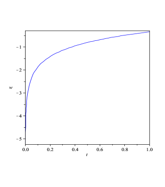
Figure 1: Dynamics of the equation of state parameter. It is possible to realize phantom divide line crossing in this setup. The crossing is possible from $\omega<-1$ to $\omega>-1$, a typical behavior of bouncing solutions.

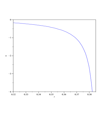
Figure 2: Crossing of the phantom divide line from quintessence ($\omega>-1$) to phantom phase ($\omega<-1$). This type of crossing behavior is supported observationally.

5 The Minimal Theory

To have a more complete discussion, we study dynamics of the equation of state parameter for a GBIG theory where a quintessence field is minimally coupled to induced gravity on the brane.

5.1 Minkowski Bulk with a Tensionless Brane

For the case with Minkowski bulk ($\psi=0$) and a tensionless brane ($\sigma=0$), the Friedmann equation is given as follows [20,21]

$$(1+\gamma h^{2})^{2}h^{2}=\bigg{[}h^{2}-(\mu+\bar{\mu})\bigg{]}^{2},$$ (30)

from which we can deduce

$$\mu+\bar{\mu}=h^{2}-h(\gamma h^{2}+1).$$ (31)

Since $(\mu+\bar{\mu})_{\infty}=0$, from equation (31) it follows that

$$\gamma=\frac{h_{\infty}-1}{h_{\infty}^{2}}.$$ (32)

We note that $\gamma$ is constraint by recent observational data from SNIa+LSS+H(z) combined dataset so that $\gamma=0.000_{-0.000}^{+0.003}$   [29]. By expanding $\mu+\bar{\mu}$ to first order in   $h^{2}-h_{\infty}^{2}$, we find

$$h^{2}=h_{\infty}^{2}+\frac{2h_{\infty}}{2-h_{\infty}}(\mu+\bar{\mu}).$$ (33)

Then we can obtain the following effective Newton’s constant

$$G_{eff}=\Big{(}\frac{h_{\infty}}{2-h_{\infty}}\Big{)}\frac{G_{5}}{r},$$ (34)

where $G_{5}=\kappa_{5}^{2}/8\pi$ and $G_{eff}=\kappa_{4}^{2}/8\pi$ are five-and four-dimensional gravitational constants respectively. From this equation we obtain

$$M_{5}^{3}\simeq\Big{(}\frac{h_{\infty}}{2-h_{\infty}}\Big{)}\frac{M_{p}^{2}}{r}.$$ (35)

The effective dark energy density is given by

$$\rho=3(8\pi G_{eff})^{-1}\frac{h^{2}}{r^{2}}.$$ (36)

So from equation (34) we obtain

$$\rho=\frac{3}{r\kappa_{5}^{2}}(\frac{2-h_{\infty}}{h_{\infty}})$$ (37)

Using the conservation equation, $\dot{\rho}+3H\rho(1+\omega)=0$,  we find

$$p=-\frac{1}{\kappa_{5}^{2}}(2\dot{h}+\frac{3h^{2}}{r})(\frac{2-h_{\infty}}{h_{\infty}}).$$ (38)

Hence, the equation of state parameter of the model is given as follows

$$\omega=-1-\frac{2r\dot{h}}{3h^{2}}$$ (39)

This equation of state parameter has the potential to describe a variety of cosmologically interesting cases. For instance, for a model universe with $a(t)\propto\ln t$ where $t$ is the cosmic time, this model has the potential to realize phantom divide line crossing. Also for models such as $a(t)=a_{0}\Big{(}t^{2}+\frac{t_{0}}{1-\nu}\Big{)}^{\frac{1}{1-\nu}}$, that are phenomenologically reliable [30], this crossing is possible too ( see figure $2$).

5.2 AdS bulk with brane tension

For the case with AdS bulk ($\psi\neq 0$) and brane tension ($\sigma\neq 0$), the Friedmann equation is as follows

$$\bigg{[}1+\gamma(h^{2}+\frac{\psi}{2})\bigg{]}^{2}(h^{2}-\psi)=\bigg{[}h^{2}-(\mu+\bar{\mu}+\sigma)\bigg{]}^{2},$$ (40)

which can be rewritten as follows

$$\mu+\bar{\mu}=h^{2}-\sigma-\bigg{[}1+\gamma(h^{2}+\frac{\psi}{2})\bigg{]}(h^{2}-\psi)^{\frac{1}{2}}.$$ (41)

Since $(\mu+\bar{\mu})_{\infty}=0$ , from this equation we find

$$\gamma=\frac{h_{\infty}^{2}-\sigma-(h_{\infty}^{2}-\psi)^{\frac{1}{2}}}{(h_{\infty}^{2}+\frac{\psi}{2})(h_{\infty}^{2}-\psi)^{\frac{1}{2}}}.$$ (42)

By expanding  $\mu+\bar{\mu}$ to first order in  $h^{2}-h_{\infty}^{2}$, we find

$$\mu+\bar{\mu}=(h^{2}-h_{\infty}^{2})(h_{\infty}^{2}+\frac{\psi}{2})^{-1}(h_{\infty}^{2}-\psi)^{-1}\Bigg{\{}\frac{1}{2}(h_{\infty}^{2}+\frac{\psi}{2})[\sigma+h_{\infty}^{2}-2\psi]+(h_{\infty}^{2}-\psi)[-h_{\infty}^{2}+\sigma+(h_{\infty}^{2}-\psi)^{\frac{1}{2}}]\Bigg{\}},$$ (43)

which can be rewritten as follows

$$h^{2}=h_{\infty}^{2}+(h_{\infty}^{2}+\frac{\psi}{2})(h_{\infty}^{2}-\psi)(\mu+\bar{\mu})\Bigg{\{}\frac{1}{2}(h_{\infty}^{2}+\frac{\psi}{2})(\sigma+h_{\infty}^{2}-2\psi)(h_{\infty}^{2}-\psi)[-h_{\infty}^{2}+\sigma+(h_{\infty}^{2}-\psi)^{\frac{1}{2}}]\Bigg{\}}^{-1}.$$ (44)

By comparing this relation with equation (6), we find the following relation for 4-dimensional effective Newtonian gravitational constant

$$G_{eff}=\Bigg{\{}\frac{1}{2}(h_{\infty}^{2}+\frac{\psi}{2})(h_{\infty}^{2}-\psi)\Bigg{(}\frac{1}{2}(h_{\infty}^{2}+\frac{\psi}{2})(\sigma+h_{\infty}^{2}-2\psi)(h_{\infty}^{2}-\psi)[-h_{\infty}^{2}+\sigma+(h_{\infty}^{2}-\psi)^{\frac{1}{2}}]\Bigg{)}^{-1}\Bigg{\}}\frac{G_{5}}{r}.$$ (45)

Now the relation between   $M_{5}^{3}$  and  $M_{p}^{2}$   reads as follows

$$M_{5}^{3}=\Bigg{(}\frac{1}{2}(h_{\infty}^{2}+\frac{\psi}{2})(h_{\infty}^{2}-\psi)\Bigg{\{}\frac{1}{2}(h_{\infty}^{2}+\frac{\psi}{2})(\sigma+h_{\infty}^{2}-2\psi)(h_{\infty}^{2}-\psi)[-h_{\infty}^{2}+\sigma+(h_{\infty}^{2}-\psi)^{\frac{1}{2}}]\Bigg{\}}^{-1}\Bigg{)}\frac{M_{p}^{2}}{r}$$ (46)

The holographic dark energy density and pressure of this model are given by

$$\rho=\frac{6h^{2}}{\kappa_{5}^{2}r}(h_{\infty}^{2}+\frac{\psi}{2})^{-1}(h_{\infty}^{2}-\psi)^{-1}\Bigg{\{}\frac{1}{2}(h_{\infty}^{2}+\frac{\psi}{2})(\sigma+h_{\infty}^{2}-2\psi)(h_{\infty}^{2}-\psi)[-h_{\infty}^{2}+\sigma+(h_{\infty}^{2}-\psi)^{\frac{1}{2}}]\Bigg{\}},$$ (47)

and

$$p=-\frac{2}{\kappa_{5}^{2}}(h_{\infty}^{2}+\frac{\psi}{2})^{-1}(h_{\infty}^{2}-\psi)^{-1}\Bigg{[}(2\dot{h}+\frac{3h^{2}}{r})\bigg{\{}\frac{1}{2}(h_{\infty}^{2}+\frac{\psi}{2})(\sigma+h_{\infty}^{2}-2\psi)(h_{\infty}^{2}-\psi)[-h_{\infty}^{2}+\sigma+(h_{\infty}^{2}-\psi)^{\frac{1}{2}}]\bigg{\}}\Bigg{]}$$ (48)

respectively. The equation of state parameter of the holographic dark energy component now is given by

$$\omega=-1-\frac{2r\dot{h}}{3h^{2}}$$ (49)

where $h$ is given by equation (44). This model accounts for crossing of the cosmological constant line if we set for instant

$$a(t)=a_{0}\Big{(}t^{2}+\frac{t_{0}}{1-\nu}\Big{)}^{\frac{1}{1-\nu}}.$$

Figure $2$ shows the realization of the phantom divide line crossing again from $\omega<-1$ to $\omega>-1$ in this setup.

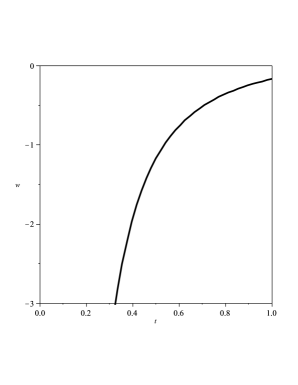
Figure 3: Dynamics of the equation of state parameter. It is possible to realize phantom divide line crossing in this setup.

We note that one important point in this DGP-inspired model is the issue of stability of the self-accelerated solutions. It has been shown that the self-accelerating branch of the DGP model contains a ghost at the linearized level [31]. The ghost carries negative energy density and it leads to the instability of the spacetime. The presence of the ghost can be related to the infinite volume of the extra-dimension in DGP setup. It is shown also that the introduction of the Gauss-Bonnet term in the bulk does not help to overcome this problem [32]. In fact, it is still unclear what is the end state of the ghost instability in self-accelerated branch of the DGP inspired models (for more details see [31]). On the other hand, non-minimal coupling of the scalar field and induced gravity provides a new degree of freedom which requires special fine tuning and this may provide a suitable basis to treat ghost instability. Lorentz invariance violating scenarios are other alternative paradigm which may shed light in this problem due to their wider parameter spaces [33]. As we have shown here, non-minimal coupling of the scalar field and induced gravity has the capability to account for bouncing solutions. It seems that this additional degree of freedom has also the capability to provide the background for a reliable solution to ghost instability. However, it is not trivial at this level and need further justification.

6 Summary and Conclusions

DGP model provides an IR modification of the general relativity. On the other hand, at the UV limit, stringy effects play important role. In this viewpoint, to discuss both UV and IR limit of a braneworld scenario simultaneously, the DGP model is not sufficient alone and one should incorporate stringy effects via inclusion of the Gauss-Bonnet term in the bulk action. The presence of GB term removes the big bang singularity, and the universe starts with an initial finite density [20,21]. Non-minimal coupling of scalar field and induced gravity on the brane which is motivated from several compelling reasons, controls the value of the initial density in a finite big bang cosmology on the brane [21]. In this paper, we have constructed a holographic picture of dark energy model by incorporating Gauss-Bonnet effect in a DGP braneworld model. By considering the IR cut-off of the model to be the crossover scale of the theory, we have obtained dynamics of the equation of state parameter of the holographic dark energy component. By adopting a suitable ansatz, we have shown that this model accounts for phantom divide line crossing in a wide range of the parameter space. Then we have studied the minimal case with detailed by considering two possible geometry of the bulk manifold and brane tension. In these case also there is crossing of the phantom divide line by adopting suitable ansatz. One of the main outcome of our analysis is the implication of the non-minimal coupling on the bouncing cosmologies. In the bouncing universe, the equation of state parameter of the matter content, $\omega$, must transit from $\omega<-1$ to $\omega>-1$. In our framework, as figure $1$ and $2$ show, this condition is possible to be realized and therefore our model essentially supports bouncing solutions. Another important point is the fact that inclusion of the non-minimal coupling of the scalar field and induced gravity on the brane in the presence of the Gauss-Bonnet term could be used to fine-tune braneworld cosmological models in the favor of the recent observational data. In this manner it is possible to find a severe constraint on the value of the non-minimal coupling in the spirit of scalar-tensor theories. Finally, the issue of ghost instabilities in the self-accelerated solutions and possible impacts of the Gauss-Bonnet term and non-minimal coupling on this issue are addressed here.

References

- [1] S. Perlmutter et al, Astrophys. J. 517 (1999) 565; A. G. Riess et al, Astron. J. 116 (1998) 1006; A. D. Miller et al, Astrophys. J. Lett. 524 (1999) L1; P. de Bernardis et al, Nature 404 (2000) 955; S. Hanany et al, Astrophys. J. Lett. 545 (2000) L5; D. N. Spergel et al, Astrophys. J. Suppl. 148 (2003) 175; L. Page et al, Astrophys. J. Suppl. 148 (2003) 233; G. Hinshaw et al, [WMAP Collaboration], [arXiv:0803.0732]; D. N. Spergel et al, Astrophys. J. Suppl. 170 (2007) 377; G. Hinshaw et al, Astrophys. J. Suppl. 170 (2007) 288; L. Page et al, Astrophys. J. Suppl. 170 (2007) 335; A. G. Reiss et al, Astrophys. J 607 (2004) 665; S. W. Allen et al, Mon. Not. R. Astron. Soc. 353 (2004) 457; E. Komatsu et al. [WMAP Collaboration], [arXiv:0803.0547].
- [2] T. Padmanabhan, [arXiv:0807.2356], see also T. Padmanabhan,[ arXiv:0705.2533].
- [3] E. J. Copeland, M. Sami and S. Tsujikawa, Int. J. Mod. Phys. D 15 (2006) 1753-1936, [arXiv:hep-th/0603057]; S. Nesseris and L. Perivolaropoulos, JCAP 0701 (2007) 018, [arXiv:astro-ph/0610092]; V. Sahni and Y. Shtanov, JCAP 0311 (2003) 014; A. Vikman, Phys. Rev. D 71 (2005) 023515, [arXiv:astro-ph/0407107]; Y. H. Wei and Y. Z. Zhang, Grav. Cosmol. 9 (2003) 307; Y.H. Wei and Y. Tian, Class. Quantum Grav. 21 (2004) 5347; F. C. Carvalho and A. Saa, Phys. Rev. D 70 (2004) 087302; F. Piazza and S. Tsujikawa, JCAP 0407 (2004) 004; I. Y. Arefeva, A. S. Koshelev and S. Y. Vernov, Phys. Rev. D 72 (2005) 064017; A. Anisimov, E. Babichev and A. Vikman, JCAP 0506 (2005)006; B. Wang, Y.G. Gong and E. Abdalla, Phys. Lett. B 624 (2005) 141; S. Nojiri and S. D. Odintsov, [arXiv:hep-th/0506212]; S. Nojiri, S. D. Odintsov and S. Tsujikawa, [arXiv:hep-th/0501025]; E. Elizalde, S. Nojiri, S. D. Odintsov and P. Wang, Phys. Rev. D 71 (2005) 103504; W. Zhao and Y. Zhang, Phys. Rev.D 73 (2006)123509; P. S. Apostolopoulos and N. Tetradis, [arXiv:hep-th/0604014]; I. Ya. Arefeva and A. S. Koshelev, [arXiv:hep-th/0605085]; A. Lue and G. D. Starkman, Phys. Rev. D 70 (2004) 101501, [arXiv:astro-ph/0408246]; S. D. Sadatian and K. Nozari, Europhys. Lett. 82 (2008) 49001; K. Nozari and M. Pourghassemi, JCAP 10 (2008) 044, [arXiv:0808.3701]; M. R. Setare and E. N. Saridakis, [ arXiv:0810.0645]; R. J. Scherrer and A. A. Sen, Phys. Rev. D 78 (2008) 067303, [arXiv:0808.1880]; F. Briscese, E. Elizalde, S. Nojiri and S. D. Odintsov, Phys. Lett. B 646 (2007) 105-111
- [4] S. Nojiri and S.D. Odintsov, Int. J. Geom. Meth. Mod. Phys. 4 (2007) 115, [hep-th/0601213]; S. Nojiri and S. D. Odintsov, [arXiv:0807.0685]; T. P. Sotiriou and V. Faraoni, [ arXiv:0805.1726]; S. Capozziello and M Francaviglia, Gen. Relativ. Gravit. 40 (2008) 357
- [5] G. Dvali, G. Gabadadze and M. Porrati, Phys. Lett. B 485 (2000) 208; G. Dvali and G. Gabadadze, Phys. Rev. D 63 (2001) 065007; G. Dvali, G. Gabadadze, M. Kolanovi and F. Nitti, Phys. Rev. D 65 (2002) 024031.
- [6] C. Deffayet, Phys. Lett. B 502 (2001) 199; C. Deffayet, G.Dvali, and G. Gabadadze, Phys. Rev. D 65 (2002) 044023; C.Deffayet, S. J. Landau, J. Raux, M. Zaldarriaga, and P. Astier, Phys. Rev. D 66 (2002) 024019.
- [7] H. Zhang and Z.-H. Zhu, Phys. Rev. D75 (2007) 023510; K. Nozari, M. R. Setare, T. Azizi and N. Behrouz, [arXiv:0810.1427]; K. Nozari and S. D. Sadatian, Eur. Phys. J. C 58 (2008) 499, [arXiv:0809.4744]
- [8] L. P. Chimento, R. Lazkoz, R. Maartens and I. Quiros, JCAP 0609 (2006) 004, [arXiv:astro-ph/0605450]; R. Lazkoz, R. Maartens and E. Majerotto, Phys. Rev. D 74 (2006) 083510, [arXiv:astro-ph/0605701]; R. Maartens and E. Majerotto, Phys. Rev. D 74 (2006) 023004, [arXiv:astro-ph/0603353]
- [9] P. S. Apostolopoulos and N. Tetradis, Phys. Rev. D 74 (2006) 064021 [arXiv:hep-th/0604014]. See also G. Dvali, G. Gabadadze, M. Kolanovic and F. Nitti, Phys. Rev.D 64 (2001) 084004, [arXiv:hep-ph/0102216]; P. S. Apostolopoulos, N. Brouzakis, E. N. Saridakis and N. Tetradis, Phys. Rev. D 72 (2005) 044013, [arXiv:hep-th/0502115]; R.-G. Cai, H.-S. Zhang and A. Wang, Commun. Theor. Phys. 44 (2005) 948, [arXiv:hep-th/0505186]
- [10] S. Capozziello, V. F. Cardone and A. Troisi, JCAP 0608 (2006) 001, [arXiv:astro-ph/0602349]; S. Capozziello, S. Nojiri and S.D. Odintsov, Phys. Lett. B 634 (2006) 93, [arXiv:hep-th/0512118]; S. Capozziello, V. F. Cardone, E. Piedipalumbo and C. Rubano, Class. Quant. Grav. 23 (2006) 1205, [arXiv:astro-ph/0507438]; S. Capozziello, V. F. Cardone, S. Carloni and A. Troisi, Int. J. Mod. Phys. D12 (2003) 1969, [arXiv:astro-ph/0307018]
- [11] M. Bouhmadi-Lopez and P. Vargas Moniz, Phys. Rev. D 78 (2008) 084019, [arXiv:0804.4484]; M. Bouhmadi-Lopez, Nucl. Phys. B 797 (2008) 78-92, [arXiv:astro-ph/0512124]; M. Bouhmadi-Lopez and A. Ferrera, JCAP 0810 (2008) 011, [arXiv:0807.4678]
- [12] D. J. Gross and J. H. Sloan, Nucl. Phys. B 291, 41 (1987)
- [13] C. Charmousis and J. F. Dufaux, Class. Quantum Grav. 19 (2002) 4671, [arXiv:hep-th/0202107]; S. C. Davis, Phys. Rev. D 67 (2003) 024030, [arXiv:hep-th/0208205]; P. Binetruy, C. Charmousis, S. C. Davis and J. F. Dufaux, Phys. Lett. B 544 (2002) 183, [arXiv:hep-th/0206089]
- [14] K. Maeda and T. Torii, Phys. Rev. D 69 (2004) 024002, [arXiv:hep-th/0309152]; see also A. N. Aliev, H. Cebeci and T. Dereli, Class. Quantum Grav. 23 (2006) 591, [arXiv:hep-th/0507121]; A. N. Aliev, H. Cebeci and T. Dereli, Class. Quant. Grav. 24 (2007) 3425, [arXiv:gr-qc/0703011]
- [15] J. E. Lidsey and N. J. Nunes, Phys. Rev. D 67 (2003) 103510, [arXiv:astro-ph/0303168]
- [16] P. S. Apostolopoulos, N. Brouzakis, N. Tetradis and E. Tzavara, Phys. Rev.D 76 (2007) 084029, [arXiv:hep-th/0708.0469]
- [17] J. F. Dufaux, J. E. Lidsey, R. Maartens and M. Sami, Phys. Rev. D 70 (2004) 083525, [arXiv:hep-th/0404161]
- [18] S. Tsujikawa, M. Sami and R. Maartens, Phys. Rev. D 70 (2004) 063525, [arXiv:astro-ph/0406078]
- [19] R. A. Brown, [arXiv:gr-qc/0701083].
- [20] R. A. Brown et al, JCAP 0511 (2005) 008, [arXiv:gr-qc/0508116]
- [21] K. Nozari and B. Fazlpour, JCAP 06 (2008) 032, [arXiv:0805.1537]
- [22] J. Khoury, B. A. Ovrut, P. J. Steinhardt, N. Turok, Phys. Rev. D 64 (2001) 123522, [arXiv:hep-th/0103239]; P. J. Steinhardt and N. Turok, Phys. Rev. D 65 (2002) 126003, [arXiv:hep-th/0111098]; L. Baum, P. H. Frampton, Phys. Rev. Lett. 98 (2007) 071301, [arXiv:hep-th/0610213]; E. N. Saridakis, Nucl. Phys. B 808 (2009) 224, [arXiv:0710.5269]
- [23] M. Bouhamdi-Lopez and D. Wands, Phys. Rev. D 71 (2005) 024010,[arXiv:hep-th/0408061]; K. Farakos and P. Pasipoularides, Phys. Rev. D 75 (2007) 024018, [ arXiv:hep-th/0610010]; M. R. Setare and E. N. Saridakis, JCAP 0903 (2009) 002, [arXiv:0811.4253]; K. Atazadeh and H. R. Sepangi, Phys. Lett. B 643 (2006) 76, [arXiv:gr-qc/0610107]; K. Nozari, Phys. Lett. B 652 (2007) 159, [arXiv:hep-th/07070719]; K. Nozari, JCAP 09 (2007) 003, [arXiv:hep-th/07081611]; M. Heydari-Fard and H. R. Sepangi, Phys. Rev. D 75 (2007) 064010, [arXiv:gr-qc/0702061]; K. Atazadeh and H. R. Sepangi, JCAP 01 (2009) 006, [arXiv:0811.3823]
- [24] V. Faraoni, Phys. Rev. D 53 (1996) 6813; V. Faraoni, Phys. Rev. D 62 (2000) 023504, [arXiv:gr-qc/0002091]
- [25] Y. Cai et al, JHEP 0710 (2007) 071 [arXiv:0704.1090]; H.-H. Xiong, Y-F. Cai, T. Qiu, Y.-S. Piao and X. Zhang, Phys. Lett. B 666 (2008) 212, [arXiv:0805.0413]; F. Finelli, JCAP 0310 (2003) 011; M. R. Setare, Phys. Lett. B 602 (2004) 1; M. R. Setare, Eur. Phys. J. C 47 (2006) 851; A. Biswas and S. Mukherji, JCAP 0602 (2006) 002; M. Bojowald, Phys. Rev. D 75 (2007) 081301(R), [arXiv:gr-qc/0608100]; T. Stachowiak and M. Szydlowski, Phys. Lett. B 646 (2007) 209, [arXiv:gr-qc/0610121]; Y.-F. Cai, T. Qiu, Y.-S. Piao, M. Li and X. Zhang, JHEP 0710 (2007)071, [arXiv:0704.1090]; A. Cardoso and D. Wands, Phys. Rev. D 77 (2008) 123538, [arXiv:0801.1667]; M. Novello and S. E. Perez Bergliaffa, [arXiv:0802.1634]
- [26] U. Alam et al, JCAP 0406 (2004) 008 [astro-ph/0403687]; D. Huterer and A. Cooray , Phys. Rev. D 71 (2005) 023506[astro-ph/0404062]; Y. Gong, Class. Quant. Grav. 22 (2005) 2121 [astro-ph/0405446]; P. Corasaniti et al, Phys. Rev. D 70 (2004) 083006[astro-ph/0406608]; S. Hannestad and E. Mortsell , JCAP 0409 (2004) 001, [astro-ph/0407259]; A. Upadhye et al, Phys. Rev. D 72 (2005) 063501, [arXiv:astro-ph/0411803]
- [27] M. Li, Phys. Lett. B 603 (2004) 1, [arXiv:hep-th/0403127]; M. Ito, Europhys. Lett. 71 (2005) 712; Y. Gong, B. Wang and Y.-Z. Zhang, Phys. Rev. D72 (2005) 043510; Y. S. Myung, Phys. Lett. B610 (2005) 18; D. Pavon, W. Zimdahl, Phys. Lett. B628 (2005) 206, [arXiv:gr-qc/0505020]; S. Nojiri and S. D. Odintsov, Gen. Rel. Grav. 38 (2006) 1285; X. Zhang and F.-Q. Wu, Phys. Rev.D 72 (2005) 043524; B. Guberina, R. Horvat and H. Nikolic, Phys. Rev.D 72 (2005) 125011; B. Wang, C.-Y. Lin and E. Abdalla, Phys. Lett. B 637 (2006) 357; B. Hu and Y. Ling, Phys. Rev.D 73 (2006) 123510, M. R. Setare and S. Shafei, JCAP 0609 (2006) 011; W. Zimdahl and D. Pavon, [arXiv:astro-ph/0606555]; H. Mohseni Sadjadi and M. Honardoost, Phys. Lett.B 647 (2007) 231; M. R. Setare, Phys. Lett. B 642 (2006) 421; B. Chen, M. Li and Y. Wang, Nucl. Phys. B 774 (2007) 256; K. Y. Kim, H. W. Lee and Y. S. Myung, Mod. Phys. Lett.A 22 (2007) 2631; M. R. Setare, [ arXiv:0708.3284]; B. Wang, C.-Y. Lin, D. Pavon and E. Abdalla, Phys. Lett.B 662 (2008) 1-6; E. N. Saridakis, Phys. Lett. B 660 (2008) 138-143; M. Li, C. Lin and Y. Wang, JCAP 05 (2008) 023; Y. S. Myung and M.-G. Seo, Phys. Lett.B 671 (2009) 435; R. Horvat, JCAP 0810 (2008) 022; M. R. Setare and E. N. Saridakis, [arXiv:0810.0645]; H. Wei, [ arXiv:0902.2030]; H. Mohseni Sadjadi, [arXiv:0902.2462]
- [28] E. N. Saridakis, [arXiv:0712.2672]; E. N. Saridakis, Phys. Lett. B 661 (2008) 335, [ arXiv:0712.3806]; M. R. Setare and E. N. Saridakis, Phys. Lett.B 670 (2008) 1-4, [arXiv:0810.3296]
- [29] J. H. He et al, Phys. Lett. B 654 (2007) 133, [arXiv:gr-qc/0707.1180]
- [30] Y.-Fu. Cai, T. Qiu, Y.-S. Piao, M. Li and X. Zhang, JHEP 0710 (2007) 071
- [31] K. Koyama, Class. Quantum Grav. 24 (2007) R231, [arXiv:hep-th/0709.2399].
- [32] C. de Rham and A. J. Tolley, JCAP 0607 (2006) 004, [arXiv:hep-th/0605122]
- [33] K. Nozari and S. D. Sadatian, JCAP 0901 ( 2009) 005, [arXiv:0810.0765]