Wavevector-dependent spin filtering and spin transport through magnetic barriers in graphene

Abstract

We study the spin-resolved transport through magnetic nanostructures in monolayer and bilayer graphene. We take into account both the orbital effect of the inhomogeneous perpendicular magnetic field as well as the in-plane spin splitting due to the Zeeman interaction and to the exchange coupling possibly induced by the proximity of a ferromagnetic insulator. We find that a single barrier exhibits a wavevector-dependent spin filtering effect at energies close to the transmission threshold. This effect is significantly enhanced in a resonant double barrier configuration, where the spin polarization of the outgoing current can be increased up to 100% by increasing the distance between the barriers.

I Introduction

The electronic properties of graphenegeim ; kim have attracted in the last four years huge experimental as well as theoretical attention.reviews Besides its fundamental interest as a new type of two-dimensional electron liquid, graphene is in fact regarded as a promising material for future nanoelectronic devices,reviews in particular in the field of spintronics,spintronics due to its small intrinsic spin-orbitso1 ; so2 ; so3 and hyperfine interactions.bjorn Indeed several recent experimentsexpspin1 ; expspin2 ; expspin3 ; expspin4 have by now demonstrated spin injection and detection in a single layer of graphene sandwiched between ferromagnetic metal electrodes and observed coherent spin transport over micrometer scale distances.

Motivated by these developments, in this paper we focus on the problem of spin resolved transport through magnetic nanostructures in graphene. The studies of graphene’s transport properties through magnetic barriers and more complex structures ale ; sim ; cserti ; tarun ; wolfgang ; zhai ; tahir ; masir0 ; masir1 ; masir2 ; heinzel ; kormanios ; ghosh ; luca address the problem of controlling the confinement and the transport of charge carriers by means of appropriate configurations of an external magnetic field inhomogeneous on sub-micron scales. Different types of magnetic nanostructures have been envisioned and their properties investigated, e.g., barriers ale ; masir0 ; masir1 ; masir2 , dots ale , wires tarun and superlattices. luca

In all these works the spin degree of freedom has been completely neglected. This is justified because of the smallness of both Zeeman splitting and spin-orbit couplingso1 ; so2 ; so3 in graphene. However, the continuous and rapid improvements in sample preparation and experimental technology and resolution in graphene research call for a refinement of the theoretical analysis to incorporate such finer effects. More importantly, it has recently been argued that local ferromagnetic correlations can be induced in graphene by several different mechanisms, e.g., proximity of a ferromagnetic insulator,exchange1 ; exchange2 ; exchangebil Coulomb interactions,exchangecoul presence of defects,exchangedefect application of an electric field in the transverse direction in nanoribbons.exchangeribbons The ferromagnetism leads to a spin splitting effectively similar to a Zeeman interaction but of much larger magnitude. For example, a ferromagnetic insulator deposited on top of a graphene layer has been predicted to produce a spin splitting of up to $5$  meV. exchange1 This is comparable with the orbital energy in a field of $1$ T, which is of order of $25\,$ meV, and thus may have important effects. The spin transport through ferromagnetic graphene has already received some attention,exchange1 ; exchange2 ; yokoyama ; niu ; namdo ; li but to the best of our knowledge all works so far have focussed only on spin effects and did not consider orbital effects. Aim of this paper then is to fill the gap and investigate this problem by fully taking into account the quasiparticle’s spin dynamics as well as its orbital motion in an inhomogeneous magnetic field.

In this paper we shall focus on the effects of Zeeman and exchange spin splitting and postpone the interesting problem of spin-orbit coupling to a future work. We show that the spin-resolved transmissions exhibit a strong dependence on the incidence angle, which allows in principle for a selective transmission of spin-up and spin-down electrons. This effect can be qualitatively understood by a simple semiclassical argument. The bending of the electron trajectories under the barrier depends on the energy and thus, in the presence of spin splitting, is different for the two spin projections. The magnitude of the polarization that can be achieved depends on the spin splitting and can be very large in the presence of a large splitting, as, e.g., that originating from a proximity-induced exchange field. Moreover, in a resonant double barrier configuration, the polarization can be enhanced by increasing the distance between the barriers. In this case, in fact, even for relatively small splitting there exists an energy range where the polarization reaches values close to one for large enough distance.

While there exist several experimental techniques to produce magnetic barriers, for concreteness we shall have in mind the case of the fringe fields created by a ferromagnetic stripe deposited on top of the graphene sample. The magnetic field generated by the stripe is known analytically. ibrahim The corresponding vector potential in the Landau gauge can be written as ${\bf A}=A(x,z)\hat{y}$, where

$$A(x,z)=\left[\int_{-\infty}^{x}B_{z}(x^{\prime},0)dx^{\prime}-\int_{0}^{z}B_{x}(x,z^{\prime})dz^{\prime}\right],$$ (1)

and we assume that the system is translationally invariant in the $y$ direction. We shall neglect possible corrugations of graphene and assume that it lies flat in the $z=0$ plane. Then the orbital dynamics is only affected by the perpendicular component $B_{z}$, while both $B_{x}$ and $B_{z}$ contribute to the Zeeman interaction. In addition we shall also include in the Zeeman term the effects of a possible exchange field. exchange1 ; exchange2

The transport properties of such structures can be calculated by means of the Landauer-Büttiker formalism in terms of the spin-resolved transmission matrix $t_{\sigma\sigma^{\prime}}$, which gives the probability amplitude for a quasiparticle incident on the magnetic structure from the left with spin projection $\sigma^{\prime}$ to be transmitted with spin $\sigma$. zhai2005b ; zhai2006 ; nikolic ; ratchet The matrix $t_{\sigma\sigma^{\prime}}$ depends on particle’s energy $E$ and incidence angle $\phi$ (see below) and must satisfy certain general symmetry requirements.zhai2005b We shall be interested in the spin-resolved conductances

$$G_{\sigma\sigma^{\prime}}=G_{0}\int^{\pi/2}_{-\pi/2}d\phi\,\cos\phi\,|t_{\sigma\sigma^{\prime}}|^{2},$$ (2)

and, with total conductance $G=\sum_{\sigma\sigma^{\prime}}G_{\sigma\sigma^{\prime}}$ and spin quantization axis along the $x$ direction, the polarization vector of transmitted current for a spin-unpolarized incident current nikolic

$${\cal P}_{x}=\frac{G_{0}}{G}\,\sum_{\sigma\sigma^{\prime}}\sigma|t_{\sigma\sigma^{\prime}}|^{2},$$ (3)

$${\cal P}_{y}=\frac{2G_{0}}{G}\,\Re\sum_{\sigma}t_{\uparrow\sigma}t^{*}_{\downarrow\sigma},$$ (4)

$${\cal P}_{z}=\frac{2G_{0}}{G}\,\Im\sum_{\sigma}t^{*}_{\uparrow\sigma}t_{\downarrow\sigma},$$ (5)

with $G_{0}=\frac{2e^{2}}{h}\frac{EL_{y}}{2\pi\hbar v_{F}}$ and their integrated value

$$P_{i}=\int^{\pi/2}_{-\pi/2}d\phi\,\cos\phi{\cal P}_{i}.$$ (6)

The rest of this paper is organized as follows. In Sec. II we discuss the spin-dependent transmission and transport through rectangular and double resonant barriers in single-layer graphene. In Sec. III we address the same problem in bilayer graphene and finally in Sec. IV we draw our conclusions.

II Single-layer graphene

Let us then start focussing on single-layer graphene. We shall neglect disorder and interaction effects and focus on a single $K$ point, where ballistic motion of charge carriers in an external magnetic field ${\bf B}=B_{x}\hat{x}+B_{z}\hat{z}$, is described by the Dirac-Weyl (DW) Hamiltonian

$$H=v_{F}{\bm{\tau}}\cdot\left({\bf p}+\frac{e}{c}{\bf A}\right)+H_{spin},$$ (7)

$$H_{spin}=\frac{g_{s}\mu_{B}}{2}{\bf B}^{eff}\cdot{\bm{\sigma}},$$ (8)

where ${\bf p}=p_{x}\hat{x}+p_{y}\hat{y}$, $v_{F}\approx 10^{6}$ m/s is the Fermi velocity, $\mu_{B}$ the Bohr magneton and $g_{s}\approx 2$ the effective Landé factor. $H_{spin}$ is the sum of the Zeeman interaction due to the magnetic field and, possibly, the proximity-induced exchange splitting, with an estimated valueexchange1 $h_{ex}\approx 5$ meV (corresponding to a Zeeman interaction with a field of about $86$ T). The vector of Pauli matrices $\bm{\tau}=\tau_{x}\hat{x}+\tau_{y}\hat{y}$ (resp. $\bm{\sigma}=\sigma_{x}\hat{x}+\sigma_{y}\hat{y}+\sigma_{z}\hat{z}$) acts in sublattice space (resp. spin space), and the wavefunction $\Psi$ is a four component object, $\Psi^{T}=(\Psi_{A\uparrow},\Psi_{B\uparrow},\Psi_{A\downarrow},\Psi_{B\downarrow}$) (the superscript $T$ denotes transposition). ${\bf A}=A(x,z)\hat{y}$ is the vector potential in the Landau gauge, with $A(x,z)$ given in Eq. (1). Since the Hamiltonian is translationally invariant in the $y$ direction and $p_{y}$ is conserved, the wavefunction can be written as $\Psi=e^{ik_{y}y}\psi$ and the DW equation reduces to a one-dimensional problem. In the following we use rescaled quantities: $x\rightarrow x\ell_{B}$, $k_{x,y}\rightarrow k_{x,y}\ell_{B}^{-1}$, $A\rightarrow AB\ell_{B}$ and $E\rightarrow E\frac{\hbar v_{F}}{\ell_{B}}$, where $B$ is a typical value of magnetic field in the problem. The magnetic length is $\ell_{B}=\left(\frac{\hbar c}{eB}\right)^{1/2}\approx 26/\sqrt{B[T]}$ nm and the orbital energy scale is $E_{m}=\frac{\hbar v_{F}}{\ell_{B}}\approx 25\sqrt{B[T]}$ meV, where $B[T]$ is the magnetic field strength expressed in Tesla.

Figure 1: Profiles of magnetic field and exchange field considered in this paper. In case (b) the exchange field is included in $B_{x}$.

II.1 Rectangular barrier

First we discuss the tunneling of a spinful DW quasiparticle through a rectangular magnetic barrier of width $W$ with an effective Zeeman field

$${\bf B}^{eff}=\lambda\,\theta(W/2-|x|)\hat{z},$$ (9)

see Fig. 1(a). The value of $\lambda$ ranges from $0.002$ for a Zeeman field of $1$ T up to $\lambda\approx 0.2$ if an exchange splitting of $5$ meV is included. With spin quantization axis along $\hat{z}$, the Hamiltonian (7) is diagonal in spin space and the two spin components can be treated separately. Accordingly, the wavefunctions are just two-component spinors. The solution to Eq. (7) with energy $E$ (assumed positive for definiteness) and spin projection $\sigma$ describing a scattering state incoming from the left can be written in the left and right ”leads” (i.e. the non-magnetic regions $x<-W/2$ and $x>W/2$) as

$$\psi_{\sigma}(x<-W/2)=\frac{1}{\sqrt{k^{i}_{x}}}{\cal W}_{0}(x)\left(\begin{array}[]{c}1\\ r_{\sigma\sigma}\end{array}\right),$$ (12)

$$\psi_{\sigma}(x>W/2)=\frac{1}{\sqrt{k^{f}_{x}}}{\cal W}_{0}(x)\left(\begin{array}[]{c}t_{\sigma\sigma}\\ 0\end{array}\right),$$ (15)

where $r_{\sigma\sigma^{\prime}}$ (resp. $t_{\sigma\sigma^{\prime}}$) is the probability amplitude for a quasiparticle incident from the left with spin projection $\sigma^{\prime}$ to be reflected (resp. transmitted) with spin $\sigma$. The matrix ${\cal W}_{0}$ is given by

$${\cal W}_{0}(x)=\left(\begin{array}[]{cc}1&1\\ e^{i\phi(x)}&-e^{-i\phi(x)}\end{array}\right)e^{i\tau_{z}k_{x}(x)x}$$ (16)

with $k_{x}(x)=\sqrt{E^{2}-[k_{y}+A(x)]^{2}}$ and $\pm e^{\pm i\phi(x)}=\frac{\pm k_{x}(x)+i[k_{y}+A(x)]}{E}$. In the leads we use the parameterization:

$$k_{y}=E\sin\phi_{i}=E\sin\phi_{f}-\Phi,$$ (17)

$$k_{x}^{i}=k_{x}(x<-W/2)=E\cos\phi_{i},$$ (18)

$$k_{x}^{f}=k_{x}(x>W/2)=E\cos\phi_{f},$$ (19)

where $\Phi=A(x>W/2)$ is the total perpendicular magnetic flux through the barrier per unit length in the $y$ direction. For $\Phi>0$ the emergence angle $\phi_{f}$ is larger than the incidence angle $\phi_{i}$. Thus a finite transmission is only possible if $\phi_{i}$ is smaller than the critical angle $\phi_{c}=\arcsin(1-\Phi/E)$. For energy smaller than the threshold value $E_{th}=|\Phi|/2$ the transmission vanishes for any incidence angle.ale ; luca This condition has a simple geometrical interpretation. In momentum space the dispersion cone after the barrier is shifted with respect to the cone in the region before the barrier by $-\Phi$ along the $k_{y}$ axis. Thus if the radius of the fixed energy circle (the Fermi line) is smaller than $\Phi/2$, the equal energy sections of the two cones do not overlap, implying that $k_{x}^{f}$ is imaginary for any $k_{y}$, i.e., the barrier is perfectly reflecting. Note that neither the emergence angle $\phi_{f}$ nor the critical angle $\phi_{c}$ depend on spin.

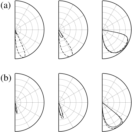
Figure 2: (a) Angular plot of the transmission through a rectangular magnetic barrier of width $W=2$ (in units of $\ell_{B}$) with $\lambda=0.2$ for spin-up (solid lines) and spin-down (dashed lines) quasiparticles at energy $E=1.05$, $1.1$, $1.7$ (from left to right, in units of $E_{m}$); (b) the same for a barrier of width $W=6$ at energy $E=3.05$, $3.1$, $3.7$. Here we set $B=1$ T, so that $E_{m}\approx 25$ meV and an energy increment of $0.1$ corresponds to $2.5$ meV.

In the barrier region $|x|<W/2$ the spin-$\sigma$ wavefunction can be written asale

$$\psi_{\sigma}(x)={\cal W}^{\sigma}_{B}(x)\left(\begin{array}[]{c}a\\ b\end{array}\right),$$ (22)

$${\cal W}^{\sigma}_{B}(x)=\left(\begin{array}[]{cc}D_{p_{\sigma}}(q)&D_{p_{\sigma}}(-q)\\ \frac{i\sqrt{2}}{E_{\sigma}}D_{p_{\sigma}+1}(q)&\frac{-i\sqrt{2}}{E_{\sigma}}D_{p_{\sigma}+1}(-q)\end{array}\right),$$ (25)

where $D_{p}(z)$ is the parabolic cylinder function, gradshteyn $q=\sqrt{2}\left[A(x)+k_{y}\right]$, $p_{\sigma}=\frac{E^{2}_{\sigma}}{2}-1$, $E_{\sigma}=E-\sigma\lambda$, and $a$ and $b$ complex amplitudes. Continuity of the wavefunction then leads to the matching condition across the magnetic barrier:

$$\left(\begin{array}[]{c}1\\ r_{\sigma\sigma}\end{array}\right)=\left(\frac{\cos\phi_{i}}{\cos\phi_{f}}\right)^{1/2}\hat{T}\left(\begin{array}[]{c}t_{\sigma\sigma}\\ 0\end{array}\right),$$ (26)

where the (spin dependent) transfer matrix $\hat{T}$ is given by

$$\hat{T}=\left[{\cal W}_{0}(-W/2)\right]^{-1}{\cal W}^{\sigma}_{B}(-W/2)\left[{\cal W}^{\sigma}_{B}(W/2)\right]^{-1}{\cal W}_{0}(W/2).$$

The transmission coefficient can directly be read from Eq. (26):

$$|t_{\sigma\sigma}|^{2}=\frac{\cos\phi_{f}}{\cos\phi_{i}}\frac{1}{\left|T_{11}\right|^{2}}.$$ (27)

The spin-resolved transmission as a function of the incidence angle is illustrated in Fig. 2 for two different barrier widths. Remarkably we find that, even though the critical angle $\phi_{c}$ is the same for both spin projections, there is a large difference between the spin-up and spin-down transmissions within an energy range $\lambda$ from the common threshold energy $E_{th}$, see Fig. 2(a). This is due to the very sharp angular and energy dependences of the transmission onset. However, this effect becomes very small as soon as $\lambda/E_{th}\ll 1$, as one can see in Fig. 2(b), where $E_{th}=3$.

Before moving to more complex structures, it is interesting to briefly consider the limit $B\rightarrow\infty$, $W\rightarrow 0$ with fixed $BW=\Phi$, where the magnetic field profile reduces to a $\delta$ function, $B(x)=\Phi\delta(x)$. Using the asymptotic behavior of the parabolic cylinder function $D_{p}(z)$ for $p\rightarrow\infty$ and $z\rightarrow 0$ with $z\sqrt{p}$ finite: watson

$$D_{-p-1}(\pm iz)=\frac{\sqrt{\pi}(p/e)^{p/2}}{\Gamma(1+p)}e^{\mp iz\sqrt{p}}\left(1+O(p^{-1/2})\right),$$

after some lengthy algebra we obtain the compact result

$${\cal W}^{\sigma}_{B}(-W/2)\left[{\cal W}_{B}^{\sigma}(W/2)\right]^{-1}\rightarrow e^{i\sigma\lambda_{z}\tau_{x}},$$ (28)

where the dimensionless Zeeman coupling is now given by $\lambda_{z}=\frac{\mu_{B}\Phi}{\hbar v_{F}}$. An elementary calculation then obtains the transmission as

$$\left|t_{\sigma\sigma}\right|^{2}=\frac{\cos\phi_{i}\cos\phi_{f}}{\cos^{2}\lambda_{z}\cos^{2}\frac{\phi_{i}+\phi_{f}}{2}+\sin^{2}\lambda_{z}\cos^{2}\frac{\phi_{i}-\phi_{f}}{2}},$$ (29)

which, in contrast to the case of a barrier of finite width, is spin independent. We note that if one solves the scattering problem by considering the Hamiltonian (7) directly with ${\bf B}^{eff}=BW\delta(x)\hat{z}$ and imposing the matching condition obtained by integrating (7) across the origin with the prescription $\delta(x)\theta(x)=\delta(x)/2$, one obtains Eq. (29) with $\lambda_{z}$ replaced by $\tilde{\lambda}_{z}=2\arctan\frac{\lambda_{z}}{2}$. The precise functional dependence of the transmission on the $\delta$-function strength depends in fact on the regularization, similarly to the case of an electrostatic barrier. kellar Since the use of the prescription $\delta(x)\theta(x)=\delta(x)/2$ in the DW first-order differential equation has been criticized,kellar in the rest of the paper we shall use Eq. (28).

II.2 The resonant double barrier

Figure 3: Illustration of the kinematics of the transmission through a resonant double magnetic barrier. The solid circles represent the constant energy contours (Fermi lines) before (resp. after) the structure (L, resp. R) or in between the barriers (C). In the leads L and R the circles are doubly spin degenerate. In C the vector potential horizontally shifts the cones along the $k_{y}$ axis, so that they are centered at $k_{x}=0$, $k_{y}=-\Phi_{1}$. The spin splitting in C vertically shifts the cones upwards (resp. downwards) for spin up (resp. spin down). The horizontal dashed line represents the fixed $y$ component of the momentum, conserved across the barriers. $\Phi=\Phi_{1}+\Phi_{2}$ is the total flux through the structure (per unit length in the $y$ direction). It is clear from the picture that if $|E-\lambda_{x}|<|k_{y}+\Phi|<|E+\lambda_{x}|$ a spin-up particle propagates in C via an evanescent wave.

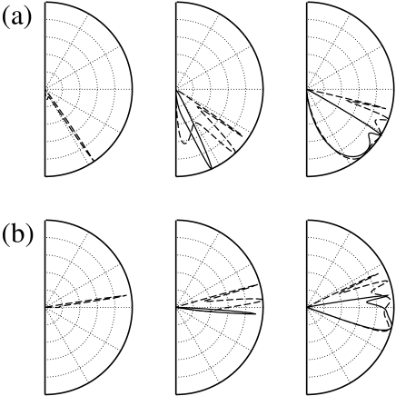
Figure 4: Angular plot of the transmission for the profile in Fig. 1(b) with $d=6$, $\lambda_{x}=0.2$, $\lambda_{z}=0$. Solid lines are for spin-up and dashed lines for spin-down. (a) Barriers of equal width $W_{1}=W_{2}=2$ and energy $E=1.02,\,1.18,\,1.5$ (from left to right); (b) the same as in (a) but for barriers of different width ($W_{1}=1$ and $W_{2}=2$).

We now discuss the case of a resonant structure consisting of two rectangular magnetic barriers with opposite signs of the magnetic field and non-vanishing in-plane Zeeman splitting in between, as illustrated in Fig. 1(b):

$${\bf B}=\left\{\begin{array}[]{rr}B\hat{z},&0<x<W_{1}\\ B_{x}\hat{x},&W_{1}<x<W_{1}+d\\ -B\hat{z},&W_{1}<x-d<W_{1}+W_{2}\\ 0,&\text{otherwise}\end{array}\right.$$ (34)

This profile should qualitatively model the realistic configuration of the stray field produced by a ferromagnetic stripe, which, in addition to the normal component, also contains an in-plane component $B_{x}$. Inclusion of this component is crucial for the proper treatment of the spin dynamics.zhai2006

First, we neglect the Zeeman term under the barriers, so that the problem is again diagonal in spin, with spin quantization axis along the $x$ direction. By way of a simple geometric argument, illustrated in Fig. 3, we argue that this structure exhibits a strong wavevector-dependent spin filtering effect. Indeed, in the region C between the barriers the dispersion cones for spin-up and spin-down particles are equally shifted by $-\Phi_{1}=-BW_{1}$ along the $k_{y}$ axis with respect to the cones in the left (L) lead. Moreover the cones are also shifted (say for $B_{x}>0$) upwards (resp. downwards) by the in-plane Zeeman splitting, so that the radius (the Fermi momentum) increases (resp. decreases) by $\lambda_{x}=\mu_{B}B_{x}/E_{m}$. As a result there exists a range of incidence angles in which the spin-down modes propagate via travelling waves in the central region, whereas the spin-up modes only exist as evanescent waves and their transmission through the structure is exponentially suppressed with the distance between the barriers. Formally, this can easily be seen from the expression of the $x$ component of the momentum in the region C, $k_{x\sigma}=\sqrt{(E-\sigma\lambda_{x})^{2}-(k_{y}+\Phi_{1})^{2}}$, which is real for $\sigma=\downarrow=-$ and pure imaginary for $\sigma=\uparrow=+$ as long as $|E-\lambda_{x}|<|k_{y}+\Phi|<|E+\lambda_{x}|$. If $|E-\lambda_{x}|>\Phi/2$ the transmission $|t_{\uparrow\uparrow}|^{2}$ at any incidence angle is fully suppressed for large enough $d$ and spin-up modes do not significantly contribute to the transport through the structure.

The exact calculation of the transmission coefficients follows the same lines as for the single rectangular barrier discussed in the previous section. The results are illustrated in Fig. 4. Fig. 4(a) shows indeed that in a certain range of incidence angles the transmission for spin-up particles practically vanishes. By changing the ratio of barrier widths $W_{1}/W_{2}$ one can also control the position of the center of this interval, as illustrated in Fig. 4(b). The width of this range clearly depends on $\lambda_{x}$. It is then crucial to have a large in-plane spin splitting if one is to observe this effect.

A simple closed formula for the transmission is easily obtained in the limit of $\delta$ barriers of equal and opposite strengths $\Phi_{1}=-\Phi_{2}=\Phi$:

$$\left|t_{\sigma\sigma}\right|^{2}=\frac{\left(\cos k_{x\sigma}d\right)^{-2}}{1+\frac{\left[k_{y}(k_{y}+\Phi)-E(E-\sigma\lambda_{x})\right]^{2}}{k_{x}^{2}k_{x\sigma}^{2}}\tan^{2}k_{x\sigma}d},$$ (35)

which explicitly exhibits the features discussed above and reproduces quite well the transmission for the case of double rectangular barriers. Resonances occur at $k_{x\sigma}d=\pi n$, with $n$ a positive integer, where $|t_{\sigma\sigma}|^{2}=1$. Upon increasing $d$, the number of resonances increases and they also become narrower. Interestingly, the positions of the resonances are different for spin-up and spin-down electrons.

Next we consider the general situation where we do not neglect the Zeeman splitting under the barriers. Then with spin quantization axis along the $x$ direction, spin-flips can take place at the barriers, hence, in contrast to the previous case, an incident particle upon transmission or reflection can change its spin state and the spin-filtering effect be spoiled. As we will see, however, the effect still survives close to some thresholds.

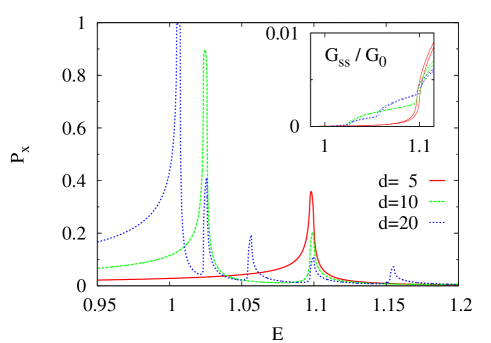
Figure 5: (Color online) Plot of the $x$ component of the polarization vector, $P_{x}$, and, in the inset, the spin-resolved conductances $G_{\uparrow\uparrow}$ and $G_{\downarrow\downarrow}$ as functions of $E$, for a structure consisting of two $\delta$ barriers with opposite signs of the magnetic field at distance $d=5$ (solid red line), $10$ (long-dashed green line), $20$ (short-dashed blue line), in units of $\ell_{B}$. The Zeeman couplings are $\lambda_{x}=-0.0025$ and $\lambda_{z}=0.005$. We take $B=1$ T and $W=2\ell_{B}\approx 50$ nm, and the energy is measured in units of $E_{m}\approx 25$ meV.

Figure 6: Maximum of the total polarization $|P(E_{M})|$ as a function of $d$ for the same structure and parameters as in Fig. 5. In the inset: plot of the energy $E_{M}$ where the peak of $|P(E)|$ is located as function of $d$.

In this case the wavefunction must be written as

$$\psi=\sum_{\sigma=\pm}\psi_{\sigma}|\sigma\rangle=\left(\begin{array}[]{c}\psi_{\uparrow}\\ \psi_{\downarrow}\end{array}\right),$$ (36)

where $|\sigma=\pm=\uparrow\downarrow\rangle$ are the eigenstates of $\sigma_{x}$ with eigenvalue $\sigma=\pm 1$ and $\psi_{\sigma}$ are two-component sublattice spinors. The solution to Eq. (7) with energy $E$ for a state incoming from the left with spin projection $\sigma$ can be written in the left and right leads as

$$\psi(x<0)=\frac{1}{\sqrt{k_{x}(x)}}{\cal W}(x)\left(\begin{array}[]{c}\delta_{\uparrow,\sigma}\\ r_{\uparrow\sigma}\\ \delta_{\downarrow,\sigma}\\ r_{\downarrow\sigma}\end{array}\right),$$ (41)

$$\psi(x>d)=\frac{1}{\sqrt{k_{x}(x)}}{\cal W}(x)\left(\begin{array}[]{c}t_{\uparrow\sigma}\\ 0\\ t_{\downarrow\sigma}\\ 0\end{array}\right),$$ (46)

where $\delta_{\sigma,\sigma^{\prime}}$ is the Kronecker delta and we introduce the $4\times 4$ matrix ${\cal W}$ given by

$${\cal W}(x)=\left(\begin{array}[]{cccc}e^{ik_{x\uparrow}(x)x}&e^{-ik_{x\uparrow}(x)x}&0&0\\ e^{i\phi_{\uparrow}(x)}e^{ik_{x\uparrow}(x)x}&-e^{-i\phi_{\uparrow}(x)}e^{-ik_{x\uparrow}(x)x}&0&0\\ 0&0&e^{ik_{x\downarrow}(x)x}&e^{-ik_{x\downarrow}(x)x}\\ 0&0&e^{i\phi_{\downarrow}(x)}e^{ik_{x\downarrow}(x)x}&-e^{-i\phi_{\downarrow}(x)}e^{-ik_{x\downarrow}(x)x}\end{array}\right),$$ (47)

with

$$k_{x\sigma} = \sqrt{(E-\sigma\lambda_{x})^{2}-(k_{y}+A)^{2}},$$ (48)

$$\pm e^{\pm i\phi_{\sigma}} = \frac{\pm k_{x\sigma}+i(k_{y}+A)}{E-\sigma\lambda_{x}}.$$ (49)

The transfer matrix is then given by

$$\hat{T}={\cal W}(0^{-})^{-1}\Omega(+){\cal W}(0^{+}){\cal W}(d^{-})^{-1}\Omega(-){\cal W}(d^{+}),$$

where the $4\times 4$ matrix $\Omega(\pm)=e^{\pm i\lambda_{z}\tau_{x}\sigma_{z}}$ (non-diagonal in spin space) implements the matching conditions at the $\delta$ barriers, and $x^{\pm}\equiv x\pm 0^{+}$. For an incident particle with spin $\sigma$ the continuity condition implies

$$\left(\begin{array}[]{c}\delta_{\uparrow,\sigma}\\ r_{\uparrow\sigma}\\ \delta_{\downarrow,\sigma}\\ r_{\downarrow\sigma}\end{array}\right)=\left(\frac{\cos\phi_{i}}{\cos\phi_{f}}\right)^{1/2}\hat{T}\left(\begin{array}[]{c}t_{\uparrow\sigma}\\ 0\\ t_{\downarrow\sigma}\\ 0\end{array}\right),$$ (58)

from which the transmission amplitudes $t_{\sigma\sigma^{\prime}}$ are easily obtained. Then using Eqs. (2)-(5) we can calculate the spin-resolved conductance and the spin polarization of the outgoing current for an unpolarized incoming current. The results are illustrated in Figs. 5-8.

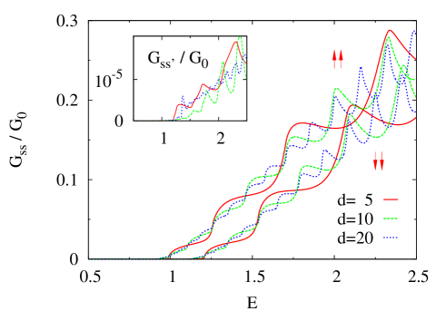
Figure 7: (Color online) Plot of the spin-resolved conductances $G_{\uparrow\uparrow}$ and $G_{\downarrow\downarrow}$ for the same structure as in Fig. 5. Here the Zeeman couplings are $\lambda_{x}=-0.2$ and $\lambda_{z}=0.005$. Same line-styles both for spin-up and spin-down. In the inset the plot of $G_{\uparrow\downarrow}=G_{\downarrow\uparrow}$ for the same parameters.

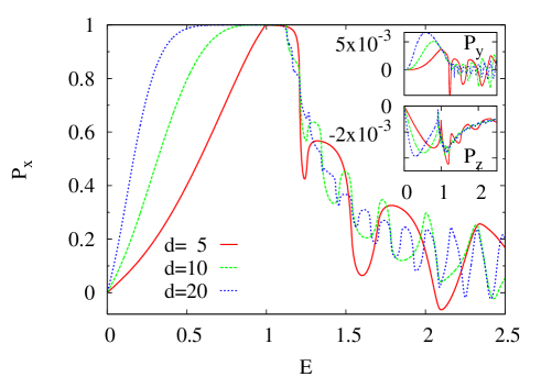
Figure 8: (Color online) Plot of the three components of the polarization vector, $P_{x}$ in the main figure, $P_{y}$ and $P_{z}$ in the insets, for the same structure and parameters as in Fig. 7.

The $x$ component of the polarization vector $P_{x}$ is plotted in Fig. 5 as a function of energy for different values of the distance $d$ between the two magnetic barriers. Just for convenience, here and below we take $B^{eff}_{x}$ negative, so that the spin-up current is favored against the spin-down current and $P_{x}$ is mostly positive. For the Zeeman couplings we use the values $\lambda_{x}=\mu_{B}B_{x}/E_{m}\approx-0.0025$ and $\lambda_{z}=\lambda_{x}\frac{B}{B_{x}}\frac{W}{\ell_{B}}\approx 0.005$ corresponding to $-B_{x}=B=1$ T and $W=2\ell_{B}\approx 50$ nm. The spin-resolved conductances $G_{\uparrow\uparrow}$ and $G_{\downarrow\downarrow}$ are plotted in the inset of Fig. 5. The conductance $G_{\downarrow\downarrow}$ is slightly lower than $G_{\uparrow\uparrow}$ while $G_{\uparrow\downarrow}=G_{\downarrow\uparrow}$ are negligibly small. There is then a very narrow energy region, close to $E=E_{th}$ ($E_{th}=1$ for $B=1$ T and $W=2\ell_{B}$), in which $G_{\uparrow\uparrow}$ and $G_{\downarrow\downarrow}$ are different (see the inset in Fig. 5), and $P_{x}$ exhibits a narrow peak. We checked that, with these values of the parameters, $P_{y}$ and $P_{z}$ are of order $10^{-3}-10^{-4}$, thus negligible, and $P_{x}$ gives the most important contribution to the total polarization $|P|=\sqrt{P_{x}^{2}+P_{y}^{2}+P_{z}^{2}}$. We have calculated $|P|$ for different values of the distance between the barriers $d$ and found that the polarization maximum increases with $d$. This behavior is clearly seen in Fig. 6, where the maximum of $|P|$ is plotted as a function of $d$. The energy $E_{M}$ at which the polarization reaches the maximum is plotted in the inset also as a function of $d$. We observe that the height of the polarization peak increases with $d$ and its position meanwhile shifts towards lower energy. From the numerical curves we can extract the following behavior for $|P(E_{M})|$ and $E_{M}$:

$$|P(E_{M})| \simeq \frac{d^{\alpha}}{C_{1}+d^{\alpha}},$$ (59)

$$E_{M} \simeq E_{th}+\frac{C_{2}}{d^{\beta}},$$ (60)

where $E_{th}=1$, $C_{1}\simeq 1090$, $C_{2}\simeq 1.3$, $\alpha\simeq 4.0$ and $\beta\simeq 1.3$. In Fig.  6 the dots represent the exact numerical results while the dashed line is the fitting curve. Upon increasing $d$ $E_{M}$ approaches the transmission threshold relative to the first barrier. From our numerical results we also observe that $C_{1}$ grows by decreasing $|\lambda_{x}|$ approximately as $C_{1}\propto|\lambda_{x}|^{-1}$, while the other parameters in Eqs. (59), (60) only weakly depend on the Zeeman couplings. For small values of $|\lambda_{x}|$ we do not have an efficient spin filter since the polarization peak occurs in a very narrow range of energy where $G_{\uparrow\uparrow}$ and $G_{\downarrow\downarrow}$ are both very small.

In the presence of an exchange field, instead, the effective Zeeman interaction also includes the exchange contribution and it is thus much larger, $\lambda_{x}\simeq-0.2$. In this case the energy range where we get polarization effects is widened and in the spin-resolved conductance plot, Fig. 7, we can now clearly distinguish $G_{\uparrow\uparrow}$ from $G_{\downarrow\downarrow}$. In particular, within a range of approximately $10$ meV we can have transmission of particles with spin-up and almost perfect reflection of particles with spin-down, realizing a very efficient spin filter. Indeed, in Fig. 8 we can see that, with a ferromagnetic region of width $d\sim 20\ell_{B}\sim 500$ nm, particles of energy $\Phi/2+\lambda_{x}\lesssim E\lesssim\Phi/2-\lambda_{x}$ (we set $\lambda_{x}$ negative), i.e. between approximately $20$ and $30$ meV, get perfectly spin-filtered upon crossing the magnetic structure. The polarization, whose largest component is $P_{x}$, reaches value one and it is sizable even for a larger range of energy. The other two components of the polarization vector, $P_{y}$ and $P_{z}$, due to the spin-flip processes at the barriers and shown in the insets of Fig. 8, remain very small, since $\lambda_{z}$ is small and confined to very narrow regions under the two thin barriers.

III Bilayer graphene

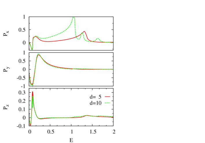
Figure 9: (Color online) Plot of the polarization vector in bilayer graphene for a structure consisting of two $\delta$ barriers with opposite signs of the magnetic field, $W=2\ell_{B}$, at distance $d=5$ (solid red line) and $10$ (long-dashed green line), in units of $\ell_{B}$. The dimensionless Zeeman couplings are $\lambda_{x}=-0.054$ and $\lambda_{z}=0.108$. The energy is given in units of $E_{b}\approx 1$ meV, for $B=1$ T.

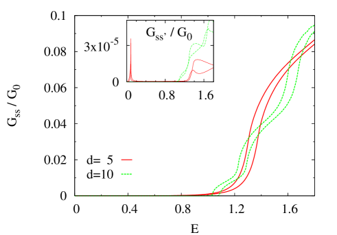
Figure 10: (Color online) Plot of the spin-resolved conductances $G_{\uparrow\uparrow}$ and $G_{\downarrow\downarrow}$ in bilayer graphene for the same structure and parameters as in Fig. 9. Same line-styles both for spin-up and spin-down. In the inset the plot of $G_{\uparrow\downarrow}$ and $G_{\downarrow\uparrow}$ for the same parameters.

In this section we consider the spin transport problem through magnetic structures in bilayer graphene. In contrast to single-layer graphene, the low-energy dynamics of charge carriers in bilayer graphene is governed by a quadratic Hamiltonian.novoselov ; falko Yet, there are important differences with respect to a standard 2DEG, since the bilayer Hamiltonian is massless and chiral, i.e., the wavefunctions for fixed spin projection are two-component spinors. The effective low-energy Hamiltonian for spinful bilayer graphene readsnovoselov ; falko ; exchangebil

$$H=\frac{1}{2m}\left(\begin{array}[]{cc}0&(\pi_{x}-i\pi_{y})^{2}\\ (\pi_{x}+i\pi_{y})^{2}&0\end{array}\right)+H_{spin},$$ (61)

with effective mass $m\approx 0.054\,m_{e}$ ($m_{e}$ is the electron mass in vacuum) and $\pi_{x,y}=p_{x,y}+\frac{e}{c}A_{x,y}$, and $H_{spin}$ was defined in Eq. (8). The possibility of inducing an exchange coupling by proximity of a ferromagnetic insulator has also been discussed in bilayer graphene.exchangebil Interestingly, in this case the electronic band structure can be drastically modified and a gap may open. However, in the simplest situation, namely the bilayer sandwiched between two ferromagnetic insulators with the same orientation of the magnetization, the only effect is a spin splitting and Eq. (61) with a large in-plane Zeeman coupling is indeed the correct Hamiltonian.exchangebil Again, using $\Psi=e^{ik_{y}y}\psi$ the problem is reduced to a one-dimensional Schrödinger equation for a four-component wavefunction $\psi$. As in the previous section, all quantities are rescaled to be dimensionless, the only difference being that the energy scale $E_{m}=\hbar v_{F}/\ell_{B}$ is now replaced by $E_{b}=\hbar^{2}/2m\ell_{B}^{2}$ ($E_{b}\approx 1$ meV for $B=1$ T). Here we directly focus on the most interesting case of a double resonant barrier configuration in the limit of $\delta$ barriers of equal and opposite strength $\Phi=BW$, with in-plane spin splitting between the barriers. Several different magnetic field profiles have also been studied in Ref. masir2, but only for the spinless case. With spin quantization axis along the $x$ direction, away from the $\delta$ barriers the elementary solutions of the Schrödinger equation for spin projection $\sigma$ read

$$U_{\sigma\pm}(x) = \left(\begin{array}[]{c}1\\ \frac{\left[\pm k_{x\sigma}+i(k_{y}+A)\right]^{2}}{E-\sigma\lambda_{x}h_{ex,x}}\end{array}\right)e^{\pm ik_{x\sigma}x},$$ (64)

$$V_{\sigma\pm}(x) = \left(\begin{array}[]{c}1\\ \frac{-\left[\pm q_{x\sigma}-(k_{y}+A)\right]^{2}}{E-\sigma\lambda_{x}h_{ex,x}}\end{array}\right)e^{\pm q_{x\sigma}x},$$ (67)

where

$$k_{x\sigma}=\sqrt{(E-\sigma\lambda_{x})-(k_{y}+A)^{2}},$$ (68)

$$q_{x\sigma}=\sqrt{(E-\sigma\lambda_{x})+(k_{y}+A)^{2}},$$ (69)

with $\lambda_{x}=\mu_{B}B_{x}/E_{b}$ ($\lambda_{x}\approx-0.054$ for $B_{x}=-1$ T) and $\lambda_{z}=\mu_{B}BW/E_{b}\ell_{B}$. It is convenient to arrange the wavefunction $\psi=\psi_{\uparrow}|\uparrow\rangle+\psi_{\downarrow}|\downarrow\rangle$ and its derivative $\psi^{\prime}$ in a eight-component vector and to write it as

$$\left(\psi_{\uparrow},\psi^{\prime}_{\uparrow},\psi_{\downarrow},\psi^{\prime}_{\downarrow}\right)^{T}={\cal W}(x)A$$ (70)

where the $8\times 8$ matrix ${\cal W}(x)$ is given by

$${\cal W}(x)=\left(\begin{array}[]{cccccccc}U_{\uparrow+}&U_{\uparrow-}&V_{\uparrow+}&V_{\uparrow-}&0&0&0&0\\ U^{\prime}_{\uparrow+}&U^{\prime}_{\uparrow-}&V^{\prime}_{\uparrow+}&V^{\prime}_{\uparrow-}&0&0&0&0\\ 0&0&0&0&U_{\downarrow+}&U_{\downarrow-}&V_{\downarrow+}&V_{\downarrow-}\\ 0&0&0&0&U^{\prime}_{\downarrow+}&U^{\prime}_{\downarrow-}&V^{\prime}_{\downarrow+}&V^{\prime}_{\downarrow-}\end{array}\right),$$

and $A$ is an eight-component vector of complex amplitudes. The matching conditions at the positions $x=0,d$ of the $\delta$ barriers (i.e., continuity of the wavefunction and jump of its derivative) can compactly be written as

$$\left(\psi_{\uparrow},\psi^{\prime}_{\uparrow},\psi_{\downarrow},\psi^{\prime}_{\downarrow}\right)^{T}(0^{-})=\Omega(+)\left(\psi_{\uparrow},\psi^{\prime}_{\uparrow},\psi_{\downarrow},\psi^{\prime}_{\downarrow}\right)^{T}(0^{+}),$$

$$\left(\psi_{\uparrow},\psi^{\prime}_{\uparrow},\psi_{\downarrow},\psi^{\prime}_{\downarrow}\right)^{T}(d^{-})=\Omega(-)\left(\psi_{\uparrow},\psi^{\prime}_{\uparrow},\psi_{\downarrow},\psi^{\prime}_{\downarrow}\right)^{T}(d^{+}),$$

where the matrix $\Omega$, non-diagonal in spin-space, is given by

$$\Omega(\pm)=\left(\begin{array}[]{cccc}\tau_{0}&0&0&0\\ \mp\tau_{z}&\tau_{0}&\mp\lambda_{z}\tau_{x}&0\\ 0&0&\tau_{0}&0\\ \mp\lambda_{z}\tau_{x}&0&\mp\tau_{z}&\tau_{0}\end{array}\right).$$ (71)

Finally, the transfer matrix obtains as

$$\hat{T}={\cal W}(0^{-})^{-1}\,\Omega(+)\,{\cal W}(0^{+})\,{\cal W}(d^{-})^{-1}\,\Omega(-)\,{\cal W}(d^{+}).$$

The scattering state for a quasiparticle of energy $E>k_{y}^{2}$ and spin projection $\sigma$ incident on the structure from the left can then be written as ${\cal W}(x)L_{\sigma}$ for $x<0$ and ${\cal W}(x)R_{\sigma}$ for $x>d$, where

$$L^{T}_{\sigma}=\left(\delta_{\uparrow,\sigma},r_{\uparrow\sigma},a_{\sigma},0,\delta_{\downarrow,\sigma},r_{\downarrow\sigma},a^{\prime}_{\sigma},0\right),$$ (72)

$$R^{T}_{\sigma}=\left(t_{\uparrow\sigma},0,0,b_{\sigma},t_{\downarrow\sigma},0,0,b^{\prime}_{\sigma}\right).$$ (73)

The transmission amplitudes $t_{\sigma\sigma^{\prime}}$ are found by solving the two linear systems

$$L_{\sigma}=\hat{T}R_{\sigma},$$ (74)

for $\sigma=\uparrow/\downarrow$.( This can also be easily generalized to the case of unequal strengths of the $\delta$ barriers.) Then, from Eqs. (2)-(6) we can calculate the spin resolved conductance and the polarization.

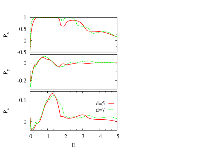
Figure 11: (Color online) Plot of the polarization in bilayer graphene, for a structure consisting of two $\delta$ barriers with opposite signs of the magnetic field, $W=2\ell_{B}$, at distance $d=5$ (solid red line) and $7$ (long-dashed green line), in units of $\ell_{B}$. The dimensionless Zeeman couplings are $\lambda_{x}=-1$ and $\lambda_{z}=0.108$. The energy is given in units of $E_{b}\approx 1$ meV for $B=1$ T.

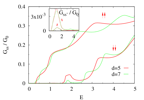
Figure 12: (Color online) Plot of the spin-resolved conductances $G_{\uparrow\uparrow}$ and $G_{\downarrow\downarrow}$ in bilayer graphene, for the same structure and parameters as in Fig. 11. Same line-styles both for spin-up and spin-down. In the inset the plot of $G_{\uparrow\downarrow}$ and $G_{\downarrow\uparrow}$ for the same parameters.

In Fig. 9 all three components of the polarization vector are shown for two different values of $d$. Looking at the structure of the polarization, we can distinguish two different behaviors at two energy scales. The first occurs close to $E\sim\lambda_{z}\simeq 0.1$ and is dominated by spin-flip processes, as one can recognize by looking at the profile of the three components of the polarization which all exhibit some features. Indeed, at this energy scale, $\lambda_{z}$ is not negligible and spin-flips may play a role. At that energy, however the conductance is almost zero, see Fig. 10, so spin-flips can hardly be detected by direct transport measurements, at least for this value of $\lambda_{z}$. The second behavior occurs close to $E\sim E_{th}=\Phi/2=1$ which is the signature of a real spin-filter effect, as one can see from the spin-resolved conductances plotted in Fig. 10. At this energy scale $\lambda_{z}$ is negligible and, in fact, $P_{y}$ and $P_{z}$, as well as $G_{\uparrow\downarrow}$ and $G_{\downarrow\uparrow}$, which are due to spin-flip processes, practically vanish, while $P_{x}$ reaches its maximum.

In the presence of a larger effective in-plane Zeeman coupling $\lambda_{x}$, possibly produced by the exchange spin splitting, the spin-filter effect is more pronounced. In Fig. 11 the polarization vector is shown for two different value of $d$, with dimensionless Zeeman couplings $\lambda_{x}=-1$ and $\lambda_{z}\simeq 0.1$. With this larger absolute value of $\lambda_{x}$ the energy range in which the spin filtering occurs is significantly widened. This is also seen in the behavior of the spin-resolved conductances in Fig. 12, which shows indeed that particles with spin-down are almost perfectly reflected by the magnetic structure for energies smaller than approximately $2-3$ meV, while spin-up particles are almost always transmitted with spin up, since the amplitude for spin-flips is very small, as shown in the inset of Fig. 12.

IV Conclusions

In conclusion, we have analyzed the spin transport problem through magnetic nanostructures in graphene. We have shown that an inhomogeneous field profile together with a strong in-plane spin splitting can produce a remarkable wavevector-dependent spin filtering effect. This effect is enhanced in a resonant barrier configuration, where the polarization can reach values up to one. This result can be understood by means of a simple kinematical analysis of the problem.

While we confined ourselves to zero temperature, we expect that the effect should be observable at finite temperature as well, as long as the temperature is smaller than the in-plane spin splitting. If the splitting originates from the exchange coupling and the estimate of Ref. exchange1, is experimentally confirmed, then there is a comfortable temperature window (say below 10 K) where the effect we discussed could in principle be observed. Other mechanisms inducing local ferromagnetic correlations in graphene could also be exploited to increase the spin splitting, thereby improving the spin filtering effect. Moreover, since the orbital dynamics and the spin dynamics in this problem are to a large extent decoupled (this would not be the case with spin-orbit coupling), we expect that the addition of a small amount of impurity scattering would not spoil the spin filtering effect, at least as long as the scatterers are enough long-range that they do not induce scattering between the two K points.

Along the same lines of this work, one could also investigate the effects of spin-orbit coupling (SOC). While the SOC has so far been estimated to be very small in graphene,so1 ; so2 ; so3 recent experimental resultsvarykhalov indicate that in quasifreestanding graphene produced on Ni(111) with intercalation of Au the Rashba effect leads to a large spin splitting of order of 13 meV. We plan to address this problem in a forthcoming work.

Finally, we hope that our paper will stimulate further experimental research on the physics and the transport properties of magnetic nanostructures in graphene.

- (1) K.S. Novoselov, A.K. Geim, S.V. Morozov, D. Jiang, Y. Zhang, S.V. Dubonos, I.V. Griegorieva, and A.A. Firsov, Science 306, 666 (2004); Nature (London) 438, 197 (2005).
- (2) Y. Zhang, Y.W. Tan, H.L. Stormer, and P. Kim, Nature (London) 438, 201 (2005).
- (3) For recent reviews, see A.K. Geim and K.S. Novoselov, Nature Mat. 6, 183 (2007); A.H. Castro Neto, F. Guinea, N.M.R. Peres, K.S. Novoselov, and A.K. Geim, Rev. Mod. Phys. 81, 109 (2009).
- (4) I. Žutić, J. Fabian, S. Das Sarma, Rev. Mod. Phys. 76, 323 (2004).
- (5) D. Huertas-Hernando, F. Guinea, and A. Brataas, Phys. Rev B 74 155426 (2006).
- (6) Hongki Min, J.E. Hill, N.A. Sinitsyn, B.R. Sahu, L. Kleinman, and A.H. MacDonald, Phys. Rev. B 74, 165310 (2006).
- (7) Y. Yao, F. Ye, X.L. Qi, S.C. Zhang, and Z. Fang, Phys. Rev. B 75, 041401(R) (2007).
- (8) B. Trauzettel, D.V. Bulaev, D. Loss, and G. Burkard, Nature Phys. 3, 192 (2007).
- (9) N. Tombros, C. Jozsa, M. Popinciuc, H.T. Jonkman, and B.J. van Wees, Nature 448, 571 (2007).
- (10) E.W. Hill, A.K.Geim, K.S. Novoselov, F. Schedin, and P. Blake, IEEE Trans. Magn. 42(10),2694 (2006).
- (11) S. Cho, Y.F. Chen, and M.S. Fuhrer, Appl. Phys. Lett. 91 123105 (2007).
- (12) M. Nishioka and A.M. Goldman, Appl. Phys. Lett. 90 252505 (2007).
- (13) A. De Martino, L. Dell’Anna, and R. Egger, Phys. Rev. Lett. 98, 066802 (2007); Solid State Commun. 144, 547 (2007).
- (14) S. Park and H.S. Sim, Phys. Rev. B 77, 075433 (2008).
- (15) P. Rakyta, L. Oroszlany, A. Kormanyos, C.J. Lambert, and J. Cserti, Phys. Rev. 77, 081403(R) (2008).
- (16) T.K. Ghosh, A. De Martino, W. Häusler, L. Dell’Anna, and R. Egger, Phys. Rev. B 77, 081404(R) (2008).
- (17) W. Häusler, A. De Martino, T. K. Ghosh, and R. Egger, Phys. Rev. B 78, 165402 (2008).
- (18) F. Zhai and K. Chang, Phys. Rev. B 77, 113409 (2008).
- (19) M. Tahir and K. Sabeeh, Phys. Rev. B 77, 195421 (2008).
- (20) M. Ramezani Masir, P. Vasilopoulos, and F.M. Peeters, Appl. Phys. Lett. 93, 242103 (2008).
- (21) M. Ramezani Masir, P. Vasilopoulos, A. Matulis, and F.M. Peeters, Phys. Rev. B 77, 235443 (2008);
- (22) M. Ramezani Masir, P. Vasilopoulos, and F.M. Peeters, Phys. Rev. B 79, 035409 (2009).
- (23) Hengyi Xu, T. Heinzel, M. Evaldsson, and I.V. Zozoulenko, Phys. Rev. B 77, 245401 (2008).
- (24) A. Kormányos, P. Rakyta, L. Oroszlány, and J. Cserti, Phys. Rev. B 78, 045430 (2008).
- (25) S. Ghosh and M. Sarma, arXiv:0806.2951.
- (26) L. Dell’Anna, and A. De Martino, Phys. Rev. B 79, 045420 (2009).
- (27) H. Haugen, D. Huertas-Hernando, and A. Brataas, Phys. Rev. B 77, 115406 (2008).
- (28) Y.G. Semenov, K.W. Kim, and J.M. Zavada, Appl. Phys. Lett. 98, 016802 (2007)
- (29) Y.G. Semenov, J.M. Zavada, and K.W. Kim, Phys. Rev. B 77, 235415 (2008).
- (30) N.M.R. Peres, F. Guinea, and A.H. Castro Neto, Phys. Rev. B 72, 174406 (2005).
- (31) O.V. Yazyev and L. Helm, Phys. Rev.B 75, 125408 (2007).
- (32) Y.-W. Son, M.L. Cohen, and S.G. Louie, Nature 444, 347 (2006).
- (33) T. Yokoyama, Phys. Rev. B 77, 073413 (2008).
- (34) Z.P. Niu, F.X. Li, B.G. Wang, L. Sheng, and D.Y. Xing, Eur. Phys. J. B 66, 245 (2008).
- (35) V. Nam Do, V. Hung Nguyen, P. Dollfus, and A. Bournel, J. Appl. Phys. 104, 063708 (2008).
- (36) Y.-X. Li, Eur. Phys. J. B 68, 119 (2009).
- (37) See for example I.S. Ibrahim and F.M. Peeters, Phys. Rev. B 52, 17321 (1995).
- (38) Feng Zhai and H. Q. Xu, Phys. Rev. Lett. 94, 246601 (2005).
- (39) Feng Zhai and H.Q. Xu, Appl. Phys. Lett. 88, 032502 (2006).
- (40) B.K. Nikolic and S. Souma, Phys. Rev. B 71, 195328 (2005).
- (41) M. Scheid, D. Bercioux, and K. Richter, New J. of Phys. 9, 401 (2007).
- (42) I.S. Gradshteyn and I.M. Ryzhik, Table of Integrals and, Series, and Products 6th ed. (Academic Press, Inc., New York, 2000).
- (43) G.N. Watson, Proc. London Math. Soc. (2) 8, 393 (1910); see also N. Schwid, Trans. Amer. Math. Soc. 37, 339 (1935).
- (44) B.H.J. McKellar and G.J. Stephenson Jr., Phys. Rev. A 36, 2566 (1987).
- (45) K.S. Novoselov et. al., Nature Phys. 2, 177 (2006).
- (46) E. McCann and V.I. Fal’ko, Phys. Rev. Lett. 96, 086805 (2006).
- (47) M.I. Katsnelson, K.S. Novoselov, and A.K. Geim, Nature Phys. 2, 620 (2006).
- (48) A. Varykhalov, J. Sánchez-Barriga, A.M. Shikin, C. Biswas, E. Vescovo, A. Rybkin, D. Marchenko, and O. Rader, Phys. Rev. Lett. 101, 157601 (2008).