Quasi-cyclic LDPC codes with high girth

Christian Spagnol (christians@rennes.ucc.ie)
Department of Electronic engineering, UCC Cork, Ireland.

Marta Rossi (marta.rossi@posso.dm.unipi.it)
Department of Mathematics and Appl., University of Milan-Bicocca, Italy.

Massimiliano Sala (msala@bcri.ucc.ie)
Department of Mathematics university of Trento, Italy /Boole Centre for Research in Informatics, UCC Cork, Ireland.

Abstract. We study a class of quasi-cyclic LDPC codes. We provide precise conditions guaranteeing high girth in their Tanner graph. Experimentally, the codes we propose perform no worse than random LDPC codes with their same parameters, which is a significant achievement for algebraic codes.

Keywords: LDPC codes, quasi-cyclic codes, Tanner graph.

1 Introduction

The LDPC codes are codes that approach optimal decoding performances, with an acceptable decoding computational cost ([1, 2, 3]). In this paper we present a class of quasi-cyclic LDPC codes and we show that we are able to guarantee some relevant properties of the codes. Experimentally, their decoding performance is comparable with the performance obtained by random LDPC codes.

Traditionally, coding theory is divided into two main research areas: algebraic coding theory and probabilistic coding theory. The former ([4]) deals with codes endowed with a nice algebraic structure, which allows both to study their internal properties and to have efficient encoding-decoding techniques, the latter deals with convolutional codes, which are very difficult to study and randomly constructed, but having superior decoding performance. However, the rediscovery of the LDPC codes by MacKay ([3]) triggered a radical change in coding theory: now we have linear block codes that may reach decoding performance close to the upper bound given by the Shannon limit ([5]). Dozens of papers have appeared since MacKay’s paper, some of them trying to endow some structure (either algebraic or geometrical) on LDPC codes. However this has seldom been successful, because the structure brings a regularity in the parity-check matrix of the code, which naturally pushes towards the creation of many dangerous small cycles in their Tanner graph. It the object of this paper to propose a family of LDPC codes, possessing an algebraic structure but not suffering from the performance limitations common to other similar families. The family of quasi-cyclic  LDPC codes are of great interest for the possibility of exploiting the structure of the parity check matrix to achieve very fast and efficient encoding and decoding. Unfortunately the BER/SNR performance of this class of codes is known to be worst than random generated LDPC codes in particular for medium/long length.

The object of this contribution is to study the family of quasi-cyclic  LDPC codes, and provide precise conditions guaranteeing high girth in the Tanner graph. Although several families of quasi-cyclic LDPC codes have been proposed, no general study on their girth properties have been published. Previous researches presented in the literature focuses on studies of the properties of particular classes of quasi-cyclic  LDPC codes constructed from circulant matrices obtained from a monomial. It is our purpose to fill this gap, by formally classify all cases when cycles of length less than $10$ may arise in the general case. Therefore, in this contribution matrices obtained from polynomial are also considered. The study is restricted to polynomials composed of two or less monomials, the reason for such limitation is the fact that circulant obtained from polynomial composed by three or more monomials internal cycles of length h $6$ always exist. Hence such polynomial are of no interest if codes with higher girth is wanted.

From the classification obtained, it is obvious how to identify necessary and sufficient conditions for any quasi-cyclic LDPC code to have girth at least $10$. Various constructions are presented that perform no worse than random LDPC codes with the same parameters, which is a significant achievement for algebraic codes.

The remainder of this paper is structured as follows:

• Section 2 provides notations, recall some relevant well-known facts and prove some simple preliminary statements;

• Section 3 deals with theclassification of the cases when cycles up to length $8$ may arise for a rather general code family;

• Section 4 improves results from Section 3 for the generic quasi-cyclic  case;

• In section 5 the existence of short cycles is linked with condition on the polynopmial representation of the circulant matrices;

• In sections 7, 8 and  9 varius subclass of quasi-cyclic  codes are studied in details and detailed conditions to avoid short cycles are given. The performances of such codes is compared with other codes,

• Finnaly in section 10 comments, conclusions, and outline some further research are presented.

2 Preliminaries and notation

In this section some known facts are recalled, some notation are given and some simple statements that will be useful later on are proved.

2.1 LDPC codes and Tanner graphs

The parity-check matrix $H=(h_{i,j})$ of any binary $[n,k,d]$ linear code $C$ may be represented by a graph $\Gamma$, known as the Tanner graph ([6, 7]). The Tanner graph is formed by two types of nodes: the “bit nodes” and the “check nodes”. Bit nodes correspond to matrix columns and check nodes correspond to matrix rows, so that there are $r=n-k$ check nodes and $n$ bit nodes. We connect the check node $i$ to the bit node $j$ if and only if the entry $h_{i,j}=1$. There is no edges connecting two check nodes or two bit nodes (this kind of graph is called a bipartite graph). In other words, $H$ is the adjacency matrix of $\Gamma$.

Example 2.1.

An example of a binary LDPC code and relative Tanner graph can be seen in Figure 1

$$\vspace*{-2cm}\mathbf{H}=\left[\begin{array}[]{cccccccccc}1&0&1&0&1&0&0&0&0&0\\ 0&1&0&1&0&1&0&0&0&0\\ 0&0&0&0&0&0&1&1&1&0\\ 0&0&1&0&1&0&0&0&0&1\\ 0&0&0&1&0&0&1&0&0&0\\ 0&0&0&0&0&0&0&1&1&1\\ \end{array}\right]$$

\psfrag{C0}{\scriptsize{$c_{0}$}}\psfrag{C1}{\scriptsize{$c_{1}$}}\psfrag{C2}{\scriptsize{$c_{2}$}}\psfrag{C3}{\scriptsize{$c_{3}$}}\psfrag{C4}{\scriptsize{$c_{2}$}}\psfrag{C5}{\scriptsize{$c_{3}$}}\psfrag{b0}{\scriptsize{$b_{0}$}}\psfrag{b1}{\scriptsize{$b_{1}$}}\psfrag{b2}{\scriptsize{$b_{2}$}}\psfrag{b3}{\scriptsize{$b_{3}$}}\psfrag{b4}{\scriptsize{$b_{4}$}}\psfrag{b5}{\scriptsize{$b_{5}$}}\psfrag{b6}{\scriptsize{$b_{6}$}}\psfrag{b7}{\scriptsize{$b_{7}$}}\psfrag{b8}{\scriptsize{$b_{8}$}}\psfrag{b9}{\scriptsize{$b_{9}$}}\psfrag{CheckNodes}{\small{Check Nodes}}\psfrag{BitNodes}{\small{Variable Nodes}}\includegraphics[width=325.215pt]{./TAnner_4cycle.eps}

Figure 1: Parity check matrix H and the associated Tanner Graph, the presence of a cycle is highlighted

Now we introduce LDPC codes - Low-Density Parity-Check codes - a class of linear error correcting codes. Historically, these codes were discovered by Gallager in 1963 in his PhD thesis [1]. These codes were largely ignored, because of some implementation issues. In the 1990’s they were rediscovered by MacKay [3] and now the research continues vigorously, with dozens of papers published every year ([8]).

Definition 2.2.

An LDPC code is a linear block code for which the parity check matrix has a low density of non-zero entries.

A $(c,s)$-regular LDPC code is a linear code whose parity check matrix $H$ contains exactly $c$ ones per column and $s$ ones per row.

We do not specify what we mean by low density because it depends on the context. For example, for a typical $(3,6)$-regular binary code (rate $1/2$) of block length $n$, there are only three ones in each column of $H$ and so the fraction of ones in this matrix is $6/n$.

The decoding algorithm for these codes is usually called the “sum-product algorithm”. We summarize some properties of these codes:

• the LDPC codes have excellent decoding performance, near to the channel capacity ([1, 3, 9]),

• the sum-product algorithm is based on the probabilities received from the channel and it may be idealized as a belief-propagation algorithm (see [10]), with information being passed and updated by the bit nodes to the check nodes and vice-versa, in a loop;

• the information propagation is heavily hindered by the presence of small cycles in the Tanner graph ([11]);

• the best LDPC codes are irregular and are created by some random-walk optimization algorithm ([5, 9, 12, 13, 14]);

• there is no known algebraic class of LDPC codes that has performance comparable to the best known LDPC codes.

There are two serious issues for a code not possessing an algebraic structure:

• the encoding process is computationally expensive,

• it is very difficult to study its properties.

There are many family of LDPC codes that have been proposed endowed with an algebraic (or geometrical) structure, but none of them has clearly shown, at present, a decoding performance comparable with the random LDPC codes (see [15, 16, 17, 18, 19, 20, 21, 22]).

2.2 Girth

Definition 2.3.

In a graph, a cycle is a path that starts from a vertex $v$ and ends in $v$. The girth of a graph is the smallest of its cycles.

Obviously the girth of a bipartite graph is always even. The girth is considered one of the important parameters of a LDPC code, it is commonly accepted that the presence of short cycles in the graph is one of the main parameters affecting the coding gain achievable by the LDPC code [23]. The dependency of the performances of a LDPC code on its girth distribution, in particular when small cycles have been avoided, is still under debate since mathematical proof has not yet been obtained. In contrast with the deteriorating effect of cycles on the performance of the LDPC codes, Etzion et al. [24, 25] proved how cycle-free graphs cannot support good codes. Still, simulations and applications have shown that the belief propagation algorithm is generally very effective, even in the presence of cycles in the graph [26, 5]. Nevertheless it is commonly accepted that the presence of short cycles in the graph is one of the main causes of reducing the coding gain achieved by the LDPC code [23], and so the girth is considered one of the significant parameters of a code.

For Tanner graphs of $(c,s)$-regular LDPC codes, it is possible to give upper bounds on the girth, see [22].

Theorem 2.4.

Consider a $(c,s)$-regular $[N,K,d]$ LDPC code. Let $R=N-K$ and $\alpha=(c-1)(s-1)$. If the girth $g\equiv 2\mod(4)$, then $g\leq 4\log_{\alpha}r+2$, otherwise $g\leq 4\log_{\alpha}r+4$.

When $r=404$ and $\alpha=(3-1)(6-1)=10$ (as for our simulation), we get in the worst case $\quad g\leq 4\log_{10}(404)+4=14$, but in practice it is very difficult to find such codes with $g\geq 10$, so that ensuring $g\geq 8$ is already interesting.

One of the most promising families of LDPC codes with a nice structure was proposed by Rosenthal and Vontobel ([22]). These are based on Tanner graphs built starting from Ramanujan graphs and hence are guaranteed to have a very high girth. Unfortunately, their decoding performance have been questioned ([27]) and it is not evident how an efficient encoding could be implemented.

There is a family of LDPC codes, which has been proposed by Fossorier ([28]), which is particularly interesting for us, because they are quasi-cyclic and so their structure is quite similar to ours. With Fossorier’s codes, it is easy to get a girth as high as $8$ or $10$. However, the construction by Fossorier does not provide codes whose Tanner graph has a girth higher than $12$, as shown by Fossorier himself in the same paper.

Another interesting construction has been provided in [21, 29]. They can get very high girth, but there are some open problems, in particular on how to get an efficient encoding.

To simplify the search for cycle in a Tanner graph representing a $\mathbf{H}$ parity check matrix, a novel and convenient definition of cycles of length $l_{c}$ in an arbitrary binary matrix is given here.

Definition 2.5.

Let $s,N,M$ be natural numbers with $s\geq 2$ and $N,M\geq 3$, and define $l_{c}=2s$. Let $B$ be any $N\times M$ matrix over $\mathbb{Z}$ ₂. A sub-set $V$ of $l_{c}$ entries of $B$ is called linked if the entries lay in $s$ columns and $s$ rows.

Definition 2.6.

Let $B$ be any $N\times M$ matrix over $\mathbb{Z}$ ₂. A sub-set $V$ of $l_{c}$ entries ($l_{c}=2s$) of $B$ is called a $2s$-cycle if :

• $V$ is linked, and

• for any $r$ such that $2\leq r<s$ there is no linked sub-set $W\subset V$ of $2r$ entries.

In order to clarify the meaning of the definitions two examples are shown in Figure 2

$$\qquad\qquad\Large{\left[\begin{array}[]{cccc}{\begin{picture}(0.0,0.0)(0.0,0.0)\put(1.0,-6.0){ \leavevmode\hbox to0.4pt{\vbox to20.32pt{\text{[drawing]}}}} \end{picture}}{\begin{picture}(0.0,0.0)(0.0,0.0)\put(1.0,1.0){ \leavevmode\hbox to17.47pt{\vbox to0.4pt{\text{[drawing]}}}} \end{picture}}1&{\begin{picture}(0.0,0.0)(0.0,0.0)\put(1.0,-6.0){ \leavevmode\hbox to0.4pt{\vbox to20.32pt{\text{[drawing]}}}} \end{picture}}1&&\\ {\begin{picture}(0.0,0.0)(0.0,0.0)\put(1.0,1.0){ \leavevmode\hbox to17.47pt{\vbox to0.4pt{\text{[drawing]}}}} \end{picture}}1&1&&\\ &&{\begin{picture}(0.0,0.0)(0.0,0.0)\put(1.0,-6.0){ \leavevmode\hbox to0.4pt{\vbox to20.32pt{\text{[drawing]}}}} \end{picture}}{\begin{picture}(0.0,0.0)(0.0,0.0)\put(1.0,1.0){ \leavevmode\hbox to17.47pt{\vbox to0.4pt{\text{[drawing]}}}} \end{picture}}1&{\begin{picture}(0.0,0.0)(0.0,0.0)\put(1.0,-6.0){ \leavevmode\hbox to0.4pt{\vbox to20.32pt{\text{[drawing]}}}} \end{picture}}1\\ &&{\begin{picture}(0.0,0.0)(0.0,0.0)\put(1.0,1.0){ \leavevmode\hbox to17.47pt{\vbox to0.4pt{\text{[drawing]}}}} \end{picture}}1&1\end{array}\right]}\qquad\qquad$$

$8$ entries linked set that

does not form a $8$-cycle

$$\qquad\qquad\Large{\left[\begin{array}[]{cccc}{\begin{picture}(0.0,0.0)(0.0,0.0)\put(1.0,-6.0){ \leavevmode\hbox to0.4pt{\vbox to20.32pt{\text{[drawing]}}}} \end{picture}}{\begin{picture}(0.0,0.0)(0.0,0.0)\put(1.0,1.0){ \leavevmode\hbox to51.61pt{\vbox to0.4pt{\text{[drawing]}}}} \end{picture}}1&&&{\begin{picture}(0.0,0.0)(0.0,0.0)\put(1.0,-18.0){ \leavevmode\hbox to0.4pt{\vbox to54.46pt{\text{[drawing]}}}} \end{picture}}1\\ {\begin{picture}(0.0,0.0)(0.0,0.0)\put(1.0,1.0){ \leavevmode\hbox to34.54pt{\vbox to0.4pt{\text{[drawing]}}}} \end{picture}}1&&{\begin{picture}(0.0,0.0)(0.0,0.0)\put(1.0,-6.0){ \leavevmode\hbox to0.4pt{\vbox to20.32pt{\text{[drawing]}}}} \end{picture}}1&\\ &{\begin{picture}(0.0,0.0)(0.0,0.0)\put(1.0,-6.0){ \leavevmode\hbox to0.4pt{\vbox to20.32pt{\text{[drawing]}}}} \end{picture}}{\begin{picture}(0.0,0.0)(0.0,0.0)\put(1.0,1.0){ \leavevmode\hbox to17.47pt{\vbox to0.4pt{\text{[drawing]}}}} \end{picture}}1&1&\\ &{\begin{picture}(0.0,0.0)(0.0,0.0)\put(1.0,1.0){ \leavevmode\hbox to34.54pt{\vbox to0.4pt{\text{[drawing]}}}} \end{picture}}1&&1\end{array}\right]}\qquad\qquad$$

$8$ entries linked set that

does form a $8$-cycle

Figure 2: Example of linked sets with $s=4,t=8$

Matrix (a) contains $8$ entries, they form a linked set since they lie in $4$ rows and $4$ columns but they do not form a $8$-cycle since they can be grouped in two smaller linked sets of $4$ elements each. Matrix (b) represents a linked set of entries that form a $8$-cycle, since the $8$ entries lie in $4$ rows and $4$ columns but there are no smaller linked sets.

Note that if a matrix column contains a point of a $2s$-cycle $V$ then it contains exactly two points of $V$. The same is true for the rows. Moreover a linked sub-set $V$ of $2s$ entries either is a $2s$-cycle or it contains at least a $2r$-cycle with $2\leq r<s$.

2.3 Circulant matrices

Binary circulant matrices are important as they form the “bricks” with which parity-check matrices for quasi-cyclic  LDPC codes are “built”.

Definition 2.7.

Let $m\geq 6$. Let $C$ be an $m\times m$ matrix over $\mathbb{F}_{2}$. $C$ is circulant if its rows are obtained by successive shifts (to the right). The matrix $C$ is weight-$l$ if the weight of any row is $l$. In case of circulant of weight-$2$, that are used extensively in this work, the polynomial representation of the first row, $p(x)\in\mathbb{F}_{2}[x]$, is called the polynomial of $C$. Let $p(x)=x^{a}+x^{b}$, with $a<b$. $s(p)=\min(b-a,a+m-b)$ is called the separation of $p$ (or of $C$).

Consider, for example, the following weight-$2$ circulant matrix.

(1) $$C=\left(\begin{array}[]{ccccc}1&1&0&0&0\\ 0&1&1&0&0\\ 0&0&1&1&0\\ 0&0&0&1&1\\ 1&0&0&0&1\\ \end{array}\right)$$

Its polynomial is $p=x+1$, with parameters $m=5$, $b=1$, $a=0$, $s(p)=1$.

Note, similar matrices can be described as an superimposition of two permutation matrices used by other authors (e.g. [30]), in such case the exponents are related to the power of the single permutation matrices, and the analysis presented in this chapter can be rewritten with such notation.

When the natural number $m$ is greater or equal to $3$ the equations:

(2) $$a\equiv b\mod(m),\qquad p(x)\equiv q(x)\mod(x^{m}+1)\,,$$

will be abbreviated with, respectively, :

(3) $$\quad a\equiv b,\qquad p(x)\equiv q(x)\,,$$

where the polynomial congruence is in $\mathbb{Z}$ ${}_{2}[x]$.

Let $p=x^{a}+x^{b}$, sometimes some statements where the role of $a$ and $b$ may be exchanged are needed. To provide a concise formulation in these cases, the notation $\epsilon(p)$ in congruences modulo $m$ is introduced. Let $f$ be any function $f:\mathbb{N}\mapsto\mathbb{Z}$, then

• $f(\epsilon(p))\equiv l$, means “$f(a)\equiv l$ or $f(b)\equiv l$”,

• $f(\epsilon(p))\not\equiv l$, means “$f(a)\not\equiv l$ and $f(b)\not\equiv l$”.

In the case of a circulant matrix of weight-$1$, $\epsilon(p)$ refers to the exponent of the monomial.

This notation is extended to the case when more polynomials, $p_{1}\ldots p_{s}$, are involved in a function, as follow. Let $p_{1}=x^{a_{1}}+x^{b_{1}},\,\ldots\,,p_{s}=x^{a_{s}}+x^{b_{s}}$. Let $f$ be any function $f:\mathbb{N}^{s}\mapsto\mathbb{Z}$. Then

• $f(\epsilon(p_{1}),\,\ldots\,,\epsilon(p_{s}))\equiv l$, means that there is a combination $(z_{1},\ldots,z_{s})$ where $z_{i}\in\{a_{i},b_{i}\}$ such that $f(z_{1},\ldots,z_{s})\equiv l$ and

• $f(\epsilon(p_{1}),\ldots,\epsilon(p_{s}))\not\equiv l$, means that for every possible combinations $(z_{1},\ldots,z_{s})$ where $z_{i}\in\{a_{i},b_{i}\}$ then $f(z_{1},\ldots,z_{s})\not\equiv l$.

Remark 2.8.

To avoid ambiguity, statements of kind: $f(\epsilon(p_{1}),\ldots\epsilon(p_{r}))\equiv f(\epsilon(p_{r+1}),\ldots,\epsilon(p_{s}))\quad$or
$f(\epsilon(p_{1}),\ldots\epsilon(p_{r}))\not\equiv f(\epsilon(p_{r+1}),\ldots,\epsilon(p_{s}))\,.$
will never be used.

Some simple facts on weight-$2$ circulant matrices are collected here. These follow directly from the circularity of the matrix.

Proposition 2.9.

Let $C=\{c_{i,j}\}$ be an $(m\times m)$ weight-$2$ circulant matrix over $\mathbb{Z}$ ${}_{2}[x]$ with polynomial $p(x)$. Then:

1. $c_{i,j}=1$ if and only if $j\equiv i+\epsilon(p)$,

2. $c_{x,y}=c_{t,y}=1$ (with $x\not=t$) if and only if $t-x\equiv\pm s(p)$,

3. $c_{x,y}=c_{x,z}=1$ (with $y\not=z$) if and only if $z-y\equiv\pm s(p)$,

4. $c_{x,y}=c_{t,y}=1$ and $c_{x,z}=c_{w,z}=1$ (with $y\not=z$, $x\not=t$, $x\not=w$) if and only if $x-t\equiv\pm s(p)$ and $w-x\equiv x-t\equiv\pm s(p)$.

Lemma 2.10.

Let $p$ and $q$ be two polynomials in $\mathbb{Z}$ ${}_{2}[x]$ with degree at most $m-1$. Then

$$s(p)=s(q)\quad\Leftrightarrow\quad s(p)\equiv\pm s(q)$$

Proof.

Note that $s(p)$ and $s(q)$ are not greater than $m/2$ and positive. ∎

Definition 2.11.

Let $m\geq 3$. Let $p$ and $q$ be two polynomials in $\mathbb{Z}$ ${}_{2}[x]$ with degree at most $m-1$. We say that $p$ is a shift of $q$ if there is $0\leq\mu\leq m-1$ s.t.

$$p\,\equiv\,x^{\mu}q\,.$$

In this case we write $p\sim q$.

Observe that $\sim$ is an equivalence relation in the set formed by all polynomials over $\mathbb{Z}$ ₂ with degree less than $m$.

Lemma 2.12.

Let $p$ and $q$ be two polynomials in $\mathbb{Z}$ ${}_{2}[x]$ with degree at most $m-1$. Then

$$s(p)=s(q)\quad\Leftrightarrow\quad s(p)\equiv\pm s(q)$$

Proof.

Note that $s(p)$ and $s(q)$ are not greater than $m/2$ and positive. ∎

There is a link between the separation of a polynomial and its roots.

Fact 2.13.

Let $m\geq 3$. Let $p$ and $q$ be two weight-$2$ polynomials in $\mathbb{Z}$ ${}_{2}[x]$ with degree at most $m-1$. Then

$$p\sim q\quad\Leftrightarrow\quad s(p)=s(q)\,.$$

Moreover, if $p$ and $q$ are both maximal or if they are both minimal, then the non-zero roots of $p$ and $q$ are the same (and with the same multiplicity) if and only if $p\sim q$.

Proof.

Let $p=x^{a_{p}}+x^{b_{p}}$ and $q=x^{a_{q}}+x^{b_{q}}$, with $a_{p}<b_{p}$ and $a_{q}<b_{q}$.

${\bf p\sim q\Rightarrow s(p)=s(q)}$.
If $p\sim q$, then $p\equiv x^{\mu}q$, for some $0\leq\mu\leq m-1$. That is, $p+x^{\mu}q=\lambda(x^{m}+1)$, for some $\lambda\in\mathbb{Z}_{2}[x]$. But $\deg(p+x^{\mu}q)\leq 2m-2$, since $\deg(p)\leq m-1$, $\partial q\leq m-1$ and $\mu\leq m-1$. Also, either $\partial\left(\lambda(x^{m}+1)\right)\geq m$ or $\lambda=0$.
There are three cases:

1. $\deg(x^{\mu}q)\leq m-1$.
   Then $\lambda=0$ and $p=x^{\mu}q$, which means

   $$b_{p}-a_{p}\equiv\pm s(p),\quad s(p)=s(x^{\mu}q)=s(x^{a_{q}+\mu}+x^{b_{q}+\mu})\,,$$

   $$s(x^{a_{q}+\mu}+x^{b_{q}+\mu})\equiv\pm\big{(}(b_{q}+\mu)-(a_{q}+\mu))\equiv\pm(b_{q}-a_{q})\equiv\pm s(q)\,,$$

   so that $s(p)\equiv\pm s(q)$ and hence $s(p)=s(q)$ (Lemma 2.12).

2. $\deg(x^{\mu}q)\geq m$ and we have $x^{\mu}q=x^{a_{q}+\mu}+x^{b_{q}+\mu}$, with $a_{q}+\mu\leq m-1$ and $b_{q}+\mu\geq m$.
   Then $x^{b_{q}+\mu}=x^{b_{q}+\mu-m}(x^{m}+1)+x^{b_{q}+\mu-m}$, so that $\lambda=x^{b_{q}+\mu-m}$ and either $a_{p}=b_{q}+\mu-m,b_{p}=a_{q}+\mu$, or $b_{p}=b_{q}+\mu-m,a_{p}=a_{q}+\mu$, which implies $s(p)\equiv\pm\left((a_{q}+\mu)-(b_{q}+\mu-m)\right)\equiv$ $\pm(a_{q}-b_{q}+m)\equiv$ $\equiv\pm(b_{q}-a_{q})\equiv\pm s(q)$ and hence $s(p)=s(q)$ (Lemma 2.12).

3. $\deg(x^{\mu}q)\geq m$ and we have $x^{\mu}q=x^{a_{q}+\mu}+x^{b_{q}+\mu}$, with $a_{q}+\mu\geq m$ and $b_{q}+\mu\geq m$.
   This case is the same as case 1), with the role of $p$ and $q$ exchanged. Since $\sim$ is an equivalence relation, we do not have to deal with it.

${\bf s(p)=s(q)\Rightarrow p\sim q}$.
If $s(p)=s(q)$, there are four cases:

• $s(p)=b_{p}-a_{p}$ and $s(q)=b_{q}-a_{q}$. Then $b_{p}-a_{p}=b_{q}-a_{q}$. We may assume $b_{q}\geq b_{p}$, so that $b_{q}-b_{p}=a_{q}-a_{p}$, i. e. $q=x^{b_{q}-b_{p}}p$.

• $s(p)=m-a_{p}+b_{p}$ and $s(q)=m-a_{q}+b_{q}$. Again $b_{p}-a_{p}=b_{q}-a_{q}$ and so we may argument as before.

• $s(p)=b_{p}-a_{p}$ and $s(q)=m-b_{q}+a_{q}$. It is enough to take $\mu=b_{p}-a_{q}=a_{p}+m-b_{q}$: $x^{\mu}(x^{a_{q}}+x^{b_{q}})=x^{b_{p}}+x^{a_{p}+m}\equiv x^{b_{p}}+x^{a_{p}}$.

• $s(p)=m-b_{p}+a_{p}$ and $s(q)=b_{q}-a_{q}$. Same argument.

We now suppose both $p$ and $q$ minimal and we want to show that $p\sim q$ if and only if they have the same non-zero roots (with the same multiplicity). The case when they are both maximal is analogous and will not be shown.
It is obvious that two polynomials $p$ and $q$ have the same non-zero roots with the same multiplicity if and only if $p=x^{i}q$, for some $i$. Assuming both $p$ and $q$ minimal, we have $p\sim q\quad\Leftrightarrow\quad p=x^{\mu}q$, and so our desired logical equivalence follows. ∎

3 Cycle configurations for generic matrices

In this section some notations, facts and lemmas useful to identify which cycles can exist in a given matrix are presented. A rather general class of matrices is studied. The general results obtained here will be specialized to the quasi-cyclic  case in following subsections.

For the remainder of this chapter, if not differently specified, $m,\alpha,\beta\gamma$ are natural numbers with $m\geq 3$, $\alpha,\beta,\gamma\geq 1$,

Definition 3.1.

Given a matrix $B$ over $\mathbb{Z}$ ₂, $B$ is said to be in $\mathcal{M}_{m,\alpha,\beta,\gamma}$ if it may be written as

$$B=\,\left[\begin{array}[]{ccc}A_{1,1}&\cdots&A_{1,\alpha\beta}\\ \vdots&\vdots&\vdots\\ A_{\alpha\gamma,1}&\cdots&A_{\alpha\gamma,\alpha\beta}\end{array}\right]\,$$

where the $A_{i,j}$’s are binary square matrices of dimension $m$. This decomposition is referred to as the standard decomposition of $B$ in $\mathcal{M}_{m,\alpha,\beta,\gamma}$. Any matrix $A_{i,j}$ is called a decomposition sub-matrix(d.s.). For any $i$ in $\{1,\ldots,\alpha\gamma\}$, that the set $\{A_{i,j}\mid 1\leq j\leq\alpha\beta\}$ is called a decomposition row(d.r.) of $B$. Similarly, for any $j$ in $\{1,\ldots,\alpha\beta\}$, the set $\{A_{i,j}\mid 1\leq i\leq\alpha\gamma\}$ is called a decomposition column(d.c.) of $B$.

The d.s.’s $\{A_{i,j}\}$ are defined unambiguously and the uniqueness of the standard decomposition in $\mathcal{M}_{m,\alpha,\beta,\gamma}$ is obvious. The term “standard decomposition” will be used rather than “standard decomposition in $\mathcal{M}_{m,\alpha,\beta,\gamma}$”. If $B\in\mathcal{M}_{m,\alpha,\beta,\gamma}$, $B$ can also be viewed as:

(4) $$B=\left[\begin{array}[]{ccc}L_{1,1}&\cdots&L_{1,\beta}\\ \vdots&\vdots&\vdots\\ L_{\gamma,1}&\cdots&L_{\gamma,\beta}\end{array}\right],\;L_{r,s}=\left[\begin{array}[]{ccc}A_{(r-1)\alpha+1,(s-1)\alpha+1}&\cdots&A_{(r-1)\alpha+1,s\alpha}\\ \vdots&\vdots&\vdots\\ A_{r\alpha,(s-1)\alpha+1}&\cdots&A_{r\alpha,s\alpha}\end{array}\right],$$

where $L_{r,s}$ is a square matrix of sub-matrices, with dimension $\alpha m$, ($1\leq r\leq\gamma$, $1\leq s\leq\beta$).

Remark 3.2.

If $H\in\mathcal{M}_{m,\alpha,\beta,\gamma}$ has full rank and $\beta>\gamma$, then it represent a binary linear code with dimension $(\beta-\gamma)m\alpha$ and length $\beta m\alpha$. The information rate is

$$\frac{K}{N}=\frac{(\beta-\gamma)m\alpha}{\beta m\alpha}=\frac{\beta-\gamma}{\beta}\,.$$

If $H\in\mathcal{M}_{m,\alpha,\beta,\gamma}$ is not full rank the rate of the code is lower and the value presented above can be considered as designed rate. Note that in some cases adding redundant rows, hence not having full, can be used as a method to improve performances tanks to the extra checks that a codeword has to satisfy.

It is clear that any rate can be achieved with this code construction by choosing $\beta$ and $\gamma$ appropriately.

Definition 3.3.

Let $B\in\mathcal{M}_{m,\alpha,\beta,\gamma}$ and let $\{A_{i,j}\}_{1\leq i\leq\alpha\gamma,1\leq j\leq\alpha\beta}$ form its standard decomposition. Define the sets of indexes $\mathcal{I}=\{i_{1},\ldots,i_{r}\}\subset\{1,\ldots,\alpha\gamma\}$ and $\mathcal{J}=\{j_{1},\ldots,j_{s}\}\subset\{1,\ldots,\alpha\beta\}$. With the notation $B_{\mathcal{I},\mathcal{J}}$ the sub-matrix of $B$ defined by the d.r.’s in $\mathcal{I}$ and the d.c.’s in $J$ is denoted. The sub-matrix $B_{\mathcal{I},\mathcal{J}}$ is said to be of type $(r,s)$ and $B_{\mathcal{I},\mathcal{J}}$ is called a decomposition minor(d.m.). Given two d.m.’s $B_{\mathcal{I},\mathcal{J}}$ and $C_{\mathcal{I^{\prime}},\mathcal{J^{\prime}}}$, they are considered equivalent if it is possible to obtain one from the other by d.r. permutations or by d.c. permutations or by both. An equivalence class is called a configuration of type $(r,s)$.

Foe example the following two matrices are decomposition minors of matrix $B$ in 4 and are equivalent configurations since $D^{\prime}$ can be obtained from $D$ by switching the first and second rows and then the first and second columns.

$$D=\left[\begin{array}[]{ccc}L_{1,2}&L_{1,4}&L_{1,6}\\ L_{2,2}&L_{2,4}&L_{2,6}\\ L_{4,2}&L_{4,4}&L_{4,6}\end{array}\right],\;D^{\prime}=\left[\begin{array}[]{ccc}L_{2,4}&L_{2,2}&L_{2,6}\\ L_{1,4}&L_{1,2}&L_{1,6}\\ L_{4,4}&L_{4,2}&L_{4,6}\end{array}\right],$$

Note that the relation defined on d.m.’s is actually an equivalence relation, so that “an equivalence class” makes sense.

The following lemma will be useful later on.

Lemma 3.4.

Let $I$ be the $m\times m$ identity matrix over $\mathbb{Z}$ ₂. Let $B\in\mathcal{M}_{m,\alpha,\beta,\gamma}$ and let $\{A_{i,j}\}$ form its standard decomposition. Suppose that there are $i$ and $j$ s.t. $A_{i,j}=I$. Let $B_{x,y}$ be an entry of $B$ included in $A_{i,j}$. Then

$$B_{x,y}=1\qquad\Leftrightarrow\qquad x\equiv y$$

Proof.

It is know that $x=x^{\prime}+(i-1)m$ and $y=y^{\prime}+(j-1)m$, with $1\leq x^{\prime}\leq m$ and $1\leq y^{\prime}\leq m$. The pair $(x^{\prime},y^{\prime})$ represents the components inside $A_{i,j}$. But $A_{i,j}$ is the identity, so that

$$B_{x,y}=1\quad\Leftrightarrow\quad x^{\prime}=y^{\prime}\quad\Leftrightarrow\quad x\equiv y$$

∎

Using this notation and the definitions of cycles on a matrix given previously 2.6, the following lemmas are obvious.

Lemma 3.5.

Let $B_{I,J}$ and $C_{I^{\prime},J^{\prime}}$ be equivalent d.m.’s of a matrix $B\in\mathcal{M}_{m,\alpha,\beta,\gamma}$. Then $B_{I,J}$ (strictly) contains a $2s$-cycle if and only if $C_{I,J}$ does.

Lemma 3.5 allows us to talk about “configuration of cycles”(see Def. 3.3), meaning equivalent decomposition minors that contain cycles of the same type.

All the possible (d.m.) configurations with $2s$-cycles are classified next.

Lemma 3.6.

With the notation introduced above, let $B\in\mathcal{M}_{m,\alpha,\beta,\gamma}$. Then the only configurations of $B$ that may (strictly) contain a $2s$-cycle are of type:

• $\begin{array}[]{cc}(1,1)&\left|A_{ij}\right|\,,\\ \end{array}$

• $\begin{array}[]{cc}(1,2)&\left|A_{i,j_{1}}A_{i,j_{2}}\right|\,,\\ \vdots&\vdots\end{array}$

• $\begin{array}[]{cc}(1,s)&\left|A_{i,j_{1}}\cdots A_{i,j_{s}}\right|\,,\\ \end{array}$

• $\begin{array}[]{cc}(2,2)&\left|\begin{array}[]{cc}A_{i_{1},j_{1}}&A_{i_{1},j_{2}}\\ A_{i_{2},j_{1}}&A_{i_{2},j_{2}}\\ \end{array}\right|\,,\\ \vdots&\vdots\\ \end{array}$

• $\begin{array}[]{cc}(2,s)&\left|\begin{array}[]{ccc}A_{i_{1},j_{1}}&\cdots&A_{i_{1},j_{s}}\\ A_{i_{2},j_{1}}&\cdots&A_{i_{2},j_{s}}\\ \end{array}\right|\,,\\ \vdots&\vdots\\ \end{array}$

• $\begin{array}[]{cc}(s-1,s-1)&\left|\begin{array}[]{ccc}A_{i_{1},j_{1}}&\cdots&A_{i_{1},j_{s-1}}\\ \vdots&&\vdots\\ \ A_{i_{s}-1,j_{1}}&\cdots&A_{i_{s}-1,j_{s-1}}\\ \end{array}\right|\,,\\ \end{array}$

• $\begin{array}[]{cc}(s-1,s)&\qquad\ \left|\begin{array}[]{ccc}A_{i_{1},j_{1}}&\cdots&A_{i_{1},j_{s}}\\ \vdots&&\vdots\\ A_{i_{s}-1,j_{1}}&\cdots&A_{i_{s}-1,j_{s}}\\ \end{array}\right|\,,\\ \end{array}$

• $\begin{array}[]{cc}(s,s)&\qquad\qquad\ \left|\begin{array}[]{ccc}A_{i_{1},j_{1}}&\cdots&A_{i_{1},j_{s}}\\ \vdots&&\vdots\\ A_{i_{s},j_{1}}&\cdots&A_{i_{s},j_{s}}\\ \end{array}\right|\,.\\ \end{array}$

Proof.

Since a $2s$-cycle $V$ needs $s$ matrix rows, it needs at most $s$ d.r’s, and analogously for the d.c.’s. So configuration $(s,s)$ is the largest that can occur. Since matrix rows (and matrix columns) can be grouped in d.r.’s (d.c.’s), any d.m. of $(s,s)$ is possible. This proves the claim. ∎

To any d.m. configuration, one or more cycle configurations may be associated. To proceed it is necessary to characterize the cycle configurations arising from the previous lemma. In order to do so, a convenient notation for a cycle configuration is presented. Any d.m. configuration in the statement of Lemma 3.6 is a sub-configuration of an $(s,s)$ configuration, which can generically be represented as

$$\left|\begin{array}[]{cccc}T_{1,1}&\cdots&T_{1,s}\\ \vdots&&\vdots\\ T_{s,1}&\cdots&T_{s,s}\\ \end{array}\right|\,,$$

where any $T_{i,j}$ is an $A_{h,k}$, for some $h$ and $k$. A numerical representation for cycles is adopted as follows. Let $V$ be any $2s$-cycle contained in the $(s,s)$ configuration as above. For any matrix $T_{i,j}$ With $t_{i,j}\geq 0$ the number of points of $V$ contained in $T_{i,j}$ is denoted. With d.r. and d.c. permutations, it can be supposes that

(5) $$t_{1,1}\geq t_{i,j},\,1\leq i,j\leq s,\quad t_{1,2}\geq t_{1,3}\geq\ldots\geq t_{1,s},\,t_{2,1}\geq t_{3,1}\geq\ldots\geq t_{s,1}\,.$$

A cycle presentation fulfilling conditions (5) will be called a (1)-presentation.

It is obvious that for a $2s$-cycle it must be:

(6) $$\sum_{1\leq i,j\leq s}t_{i,j}=2s\,.$$

For example, a $4$-cycle $V$, a $6$-cycles $\tilde{V}$, and a $8$-cycle $\bar{V}$ may be represented as

$$V=\left|\begin{array}[]{ccc}2&2\\ 0&0\\ \end{array}\right|,\qquad\tilde{V}=\left|\begin{array}[]{ccc}2&2&0\\ 0&2&0\\ 0&0&0\\ \end{array}\right|,\qquad\bar{V}=\left|\begin{array}[]{cccc}2&2&0&0\\ 0&1&1&0\\ 0&1&1&0\\ 0&0&0&0\\ \end{array}\right|,$$

and all these representations are (1)-presentations. To clarify the implications of the representation consider the following cycle configurations:

$$W=\left|\begin{array}[]{ccc}2&1\\ 0&3\\ \end{array}\right|,\qquad\tilde{W}=\left|\begin{array}[]{ccc}2&0&1\\ 2&0&1\\ 0&0&0\\ \end{array}\right|,\qquad$$

they do not form valid (1)-representations since in $W$ $t_{1,1}$ is not the maximum of the elements and in $\tilde{W}$ the elements of the first row are not ordered.

Note that cycle $\tilde{V}$ allows another (1)-presentation that is a column permutation of it:

$$\tilde{V}=\left|\begin{array}[]{ccc}2&2&0\\ 2&0&0\\ 0&0&0\\ \end{array}\right|.$$

For convenience, in a cycle presentation d.r.’s and d.c.’s containing only zeros will be dropped. The previous presentations may be written as follows

$$V=\left|\begin{array}[]{cc}2&2\\ \end{array}\right|,\qquad\tilde{V}=\left|\begin{array}[]{ccc}2&2\\ 0&2\\ \end{array}\right|,\qquad\bar{V}=\left|\begin{array}[]{ccc}2&2&0\\ 0&1&1\\ 0&1&1\\ \end{array}\right|\,.$$

The notation presented above leaves some ambiguity. In fact, for example, $t_{1,1}=2$ does not specify whether the two points in $T_{1,1}$ lie in the same cycle column or cycle row or in neither.

Remark 3.7 (Transpose).

Let $D$ be a d.m. of a matrix $B\in\mathcal{M}_{m,\alpha,\beta,\gamma}$ and $D^{T}$ its transpose. It is clear that $D$ contains a $2s$-cycle if and only if $D^{T}$ contains a $2s$-cycle. In the general case, it is not possible to obtain $D$ from $D^{T}$ by d.c. or d.r. operations, so $D$ and $D^{T}$ are not necessarily equivalent according to the definition given. However, if all cycle configurations associated to a given configuration are classified, then, automatically, all cycle configurations for its transpose are obtained (by transposing all of its cycle configurations).

Two lemmas are provided next, these are applied in the analysis of the $2s$-cycle configurations arising in Lemma 3.6.

Definition 3.8.

The row weight of a d.r. in a cycle configuration is defined as the sum of the $t_{i,j}$’s in the d.r, and similarly for the d.c.’s.

Lemma 3.9.

In any cycle configuration, column weights and row weights are even.

Proof.

By transposing, the statement for d.c.’s is true if and only if it is true for d.r.’s. It is here shown for d.r.’s. Given a d.r., if the relevant $t_{i,j}$’s sum to an odd number, then one point in not in a cycle row with another. But, by definition, any point in a 2s-cycle shares one cycle row with one and only one other point in the cycle, hence there cannot be d.r. with odd weight. ∎

Lemma 3.9 will be applied many times. To simplify the relevant notation, the phrase “Lemma 3.9 r-1” will be used meaning “Lemma 3.9 applied to the first d.r.”. Similarly with notations like “r-2”, “r-3”. The same notation is used the columns (e.g. “c-2”).

Lemma 3.10 (Isolation).

In any d.m. configuration $D$ containing a $2s$-cycle, the following situation cannot occur with $2\leq r<s$:

$$D=\left|\begin{array}[]{cc}D_{1}&0\\ 0&D_{2}\\ \end{array}\right|$$

where:

$\begin{array}[]{cc}D_{1}=\left|\begin{array}[]{cccc}T_{1,1}&\cdots&T_{1,r}\\ \vdots&&\vdots\\ T_{r,1}&\cdots&T_{r,r}\\ \end{array}\right|,&D_{2}=\left|\begin{array}[]{cccc}T_{r+1,r+1}&\cdots&T_{r+1,s}\\ \vdots&&\vdots\\ T_{s,r+1}&\cdots&T_{s,s}\\ \end{array}\right|\\ \end{array}$

Proof.

It is known, by definition 2.6, how in any row (and column) of a cycle $V$ there must be exactly two cycle points. If one cycle point lies in a d.r. of the $D_{1}$ then also the second cycle point of that d.r. must lie in $D_{1}$. Hence, for every d.r. in $D_{1}$ there are two cycle points, the same is true for the d.c.’s. So in $D_{1}$ there are $2r$ points that lie in $r$ d.r.’s and $r$ d.c.’s , hence they are linked, but $r<s$ and so this contradicts the definition of cycle given (Definitions 2.6). ∎

To ease the reading in situations where lemma 3.10 is not satisfy for a certain d.m. $D_{1}$ phrases of the type ”$D_{1}$ is isolated” are used throughout the chapter.

3.1 Possible configurations

The aim is now to determine all the possible $2s$-cycle configuration (using (1)-presentations) that can arise in a matrix. Some new terminology and lemmas are introduced first.

Definition 3.11.

The weights vector of a $2s$-cycle configuration is defined as the vector containing all the $t_{ij}$’s in such configuration.

For example the cycle configurations presented previously:

$$V=\left|\begin{array}[]{cc}2&2\\ \end{array}\right|,\qquad\tilde{V}=\left|\begin{array}[]{ccc}2&2\\ 0&2\\ \end{array}\right|,\qquad\bar{V}=\left|\begin{array}[]{ccc}2&2&0\\ 0&1&1\\ 0&1&1\\ \end{array}\right|\,.$$

have weights vectors

$$\begin{array}[]{ccc}[2,2],&[2,2,2],&[2,2,1,1,1,1].\\ \end{array}$$

Theorem 3.12.

The weights vectors that can make a $2s$-cycle configuration are all the possible combinations of numbers, that sum to $2s$ and that do not contain exactly two odd values.

Proof.

The sum of the elements in a weights vector must be $2s$ for the definition. Hence all the possible vectors that sum to $2s$ are candidate to be weights vectors of a $2s$-cycle configuration. The vectors that have two odd weights can be discharge since in such cases it is impossible to have even row weight and column weight for each d.r. and d.c.. In fact, if both sub-matrices with odd weights are in the same d.r. the two d.c.’s where they lie have odd weight, and vice-versa. ∎

The following theorem specifies which of these weights vectors can form a cycle configuration of chosen dimension.

Theorem 3.13.

An $(r,c)$ $2s$-cycle configuration can be obtained only from weights vectors that have the following characteristics:

• they contain at least $r+c-1$ elements,

• they contain no more than $\min(cr,2s)$ elements,

• the value of the biggest element is no more than $2s-2(c-1)$

Proof.

Suppose $r\leq c$, for remark 3.7 the case $r>c$ can be reduce to this by transposing the configuration. Any d.r. must have at least one element with $t_{ij}\neq 0$ otherwise it would be a $(r-1,c)$ cycle configuration, the same is true for the d.c.’s.

The value $t_{1,1}$ must not be $0$ for the definition of (1)-presentation, then for Lemma 3.10 there must be at least another d.m. with $t_{ij}\neq 0$ in the same d.r. or d.c. Suppose, without loss of generality, that $t_{1,2}\neq 0$. Applying Lemma 3.10 to the sub-matrix $[T_{1,1},\,T_{1,2}]$ implies that there must be another d.m. with $t_{i,j}\neq 0$ in the first d.r. or in one of the first two d.c.’s, otherwise $[T_{1,1},\,T_{1,2}]$ would be isolated. Assuming $t_{1,3}\neq 0$ another sub-matrix, $[T_{1,1},\,T_{1,2},\,T_{1,3}]$, is obtained. Repeating the process until all $t_{1,x}\neq 0$, $r-1$ d.r.’s that must have at least one $t_{i,j}\neq 0$ element are left, hence a total of at least $c+r-1$ weights are needed. Note that the same result will be obtained if instead of ”filling” the d.c.’s first the d.r.’s are filled, or any combination. It is obvious that any weights vector cannot have more that $2s$ values. Moreover, the sums of the elements in a weights vector is $2s$ but there cannot be more elements that d.m. hence the max number of elements in a weights vector is $min(2s,rc)$. Using the (1)-presentation then $t_{1,1}\geq t_{i,j}$ for every $i,j$, the remaining d.c. must not be zero and have at least row weight $2$. Since the sum of all row weights must be $2s$, the max value of $t_{1,1}$ is $2s-2(c-1)$. ∎

Using theorems 3.12 and 3.13 it is possible to determine the set of possible weights vectors that can be used to form a $(r,s)$ $2s$-cycle configuration. Obtaining the configurations from the weights vectors is a mater of placing the weights in such a way that they satisfy Lemma 3.9 and Lemma 3.10.

Next, an example is presented. The aim is to find which configurations of type $(4,5)$ can have $10$-cycles. The process starts by looking for all possible vectors of number that sum to $10$.

$$\begin{array}[]{l}\left[10\right],\\ \leavevmode\hbox to27.47pt{\vbox to17.47pt{\text{[drawing]}}},\\ \left[8,2\right],\leavevmode\hbox to36.91pt{\vbox to17.47pt{\text{[drawing]}}},\\ \leavevmode\hbox to27.47pt{\vbox to17.47pt{\text{[drawing]}}},\leavevmode\hbox to36.91pt{\vbox to17.47pt{\text{[drawing]}}},\left[7,1,1,1\right],\\ \left[6,4\right],\leavevmode\hbox to36.91pt{\vbox to17.47pt{\text{[drawing]}}},\left[6,2,2\right],\leavevmode\hbox to46.35pt{\vbox to17.47pt{\text{[drawing]}}},\left[6,1,1,1,1\right],\\ \leavevmode\hbox to27.47pt{\vbox to17.47pt{\text{[drawing]}}},\leavevmode\hbox to36.91pt{\vbox to17.47pt{\text{[drawing]}}},\leavevmode\hbox to36.91pt{\vbox to17.47pt{\text{[drawing]}}},\left[5,3,1,1\right],\leavevmode\hbox to46.35pt{\vbox to17.47pt{\text{[drawing]}}},\left[5,2,1,1,1\right],\left[5,1,1,1,1,1\right],\\ \left[4,4,2\right],\leavevmode\hbox to46.35pt{\vbox to17.47pt{\text{[drawing]}}},\leavevmode\hbox to36.91pt{\vbox to17.47pt{\text{[drawing]}}},\leavevmode\hbox to46.35pt{\vbox to17.47pt{\text{[drawing]}}},\left[4,3,1,1,1\right],\left[4,2,2,2\right],\leavevmode\hbox to55.8pt{\vbox to17.47pt{\text{[drawing]}}},\\ \qquad\left[4,2,1,1,1,1\right],\left[4,1,1,1,1,1,1\right],\\ \left[3,3,3,1\right],\leavevmode\hbox to46.35pt{\vbox to17.47pt{\text{[drawing]}}},\left[3,3,2,1,1\right],\left[3,3,1,1,1,1\right],\leavevmode\hbox to55.8pt{\vbox to17.47pt{\text{[drawing]}}},\left[3,2,2,1,1,1\right],\\ \qquad\left[3,2,1,1,1,1,1\right],\left[3,1,1,1,1,1,1,1\right],\\ \left[2,2,2,2,2\right],\leavevmode\hbox to65.24pt{\vbox to17.47pt{\text{[drawing]}}},\left[2,2,2,1,1,1,1\right],\left[2,2,1,1,1,1,1,1\right],\\ \qquad\left[2,1,1,1,1,1,1,1,1\right],\left[1,1,1,1,1,1,1,1,1,1\right].\end{array} \left[9,1\right] \left[8,1,1\right] \left[7,3\right] \left[7,2,1\right] \left[6,3,1\right] \left[6,2,1,1\right] \left[5,5\right] \left[5,4,1\right] \left[5,3,2\right] \left[5,2,2,1\right] \left[4,4,1,1\right] \left[4,3,3\right] \left[4,3,2,1\right] \left[4,2,2,1,1\right] \left[3,3,2,2\right] \left[3,2,2,2,1\right] \left[2,2,2,2,1,1\right] \left[9,1\right] \left[8,1,1\right] \left[7,3\right] \left[7,2,1\right] \left[6,3,1\right] \left[6,2,1,1\right] \left[5,5\right] \left[5,4,1\right] \left[5,3,2\right] \left[5,2,2,1\right] \left[4,4,1,1\right] \left[4,3,3\right] \left[4,3,2,1\right] \left[4,2,2,1,1\right] \left[3,3,2,2\right] \left[3,2,2,2,1\right] \left[2,2,2,2,1,1\right]$$

The crossed out vectors are not to be considered since they contain exactly two odd numbers. Applying Theorem 3.13 it is possible to eliminate weights vectors that do not have length between $8(=5+4-1)$ and $10(=\min(10,20))$ and that do not have max value less or equal to $2(=10-2(5-1))$. The remaining candidates are :

$$\left[2,2,1,1,1,1,1,1\right],\left[2,1,1,1,1,1,1,1,1\right],\left[1,1,1,1,1,1,1,1,1,1\right].$$

It is now necessary to place the values of the weights vectors inside the $(4,5)$ d.m.. It is now proved how the only possible configurations are :

$$\begin{array}[]{cc}1.\quad\left|\begin{array}[]{ccccc}2&1&1&0&0\\ 0&1&0&1&0\\ 0&0&1&0&1\\ 0&0&0&1&1\\ \end{array}\right|,\quad 2\quad\left|\begin{array}[]{ccccc}1&1&1&1&0\\ 1&0&0&0&1\\ 0&1&1&0&0\\ 0&0&0&1&1\\ \end{array}\right|,\end{array}$$

This can be proved with some easy considerations. There are twenty $T_{i,j}$ with $1\leq i\leq 4,1\leq j\leq 5$ . It must be $\sum_{i,j}t_{i,j}=10$, and $t_{1,1}\geq t_{i,j},$ $\forall i,\,\forall j\,s.t.\,i\leq 4,j\leq 4$ . There are five columns and for any of this column the weight must be even and not zero, (if there is a zero column then it falls in a smaller configuration), the only possibility to have a total sum of ten and column weights even is that all columns have weight $2$. Moreover, there are four rows and for any of these rows the weight must be even and not zero, (if there is a zero column then it falls in a smaller configuration), the only possibility for the total sum to be ten and row weights even is to have one row with weight $4$ and the remaining with weight $2$.

• Considering the weights vector $\left[2,2,1,1,1,1,1,1\right]$.
  An element $t_{i,j}=2$ cannot be on a d.r. of weight $2$ because both the d.c.and d.r. would be completed but this cannot be otherwise it would be isolated ( Lemma 3.10). So, both the elements $t_{i,j}=2$ must be in the same row, the only row with weight $4$. In this case such a row has weight $4$ and cannot have other non zero elements in it, but also the two columns are completed, since they have weight $2$. This situation does not satisfy Lemma 3.10, hence this weights vector does not lead to any cycle configuration of this size.

• Considering the weights vector $\left[2,1,1,1,1,1,1,1,1\right]$.
  Element $t_{1,1}=2$ since it is the max. Lemma 3.10 implies that there must be at least another non zero element in row one, but since only weight of value one are present and the row weight must be even then there must be two one elements in row one. Supposed that $t_{1,2}=t_{1,3}=1$. Considering now Lemma 3.9 applied to the remaining rows and columns configuration $1$, or a column/row permutation of it, is found.

• Considering the weights vector $\left[1,1,1,1,1,1,1,1,1,1\right]$.
  It can be supposed that the first row has weight $4$ hence it must have four elements $t_{1,j}=1$ that can be $t_{1,1}=t_{1,2}=t_{1,3}=t_{1,4}=1$. Applying Lemma 3.9 to all remaining rows and columns configuration $2$, or a column/row permutation of it, is obtained.

And this prove the claim.

3.2 4-cycle configurations for generic H matrices

In this section all the possible configurations that can give cycles of length $4$ in the case of a generic matrix are found and listed.

Theorem 3.14.

Let $B\in\mathcal{M}_{m,\alpha,\beta,\gamma}$. The only possible $4$-cycle configuration, in (1)-presentation, are as follows :

1. $(1,1)$,

   $$\left|4\right|,$$

2. $(1,2)$,

   $$\left|2\,2\right|,$$

3. $(2,2)$,

   $$\left|\begin{array}[]{cc}1&1\\ 1&1\\ \end{array}\right|.$$

Proof.

Following from Theorem 3.12 the only possible weights vectors for a 4-cycles are:

$$\begin{array}[]{ccc}[4],&[2,2],&[1,1,1,1].\\ \end{array}$$

From them it is straightforward to find the configurations listed in the statement. ∎

3.3 6-cycle configurations for generic H matrices

In this section all the possible configurations that can give cycles of length $6$ in the general case are found and listed.

Theorem 3.15.

Let $B\in\mathcal{M}_{m,\alpha,\beta,\gamma}$. The only possible $6$-cycle configurations, in (1)-presentation, are as follows :

1. $(1,1)$,

   $$\left|6\right|,$$

2. $(1,2)$,

   $$\left|\begin{array}[]{cc}4&2\\ \end{array}\right|,$$

3. $(1,3)$,

   $$\left|\begin{array}[]{ccc}2&2&2\\ \end{array}\right|,$$

4. $(2,2)$,
   

   $$\begin{array}[]{cc}4.1\left|\begin{array}[]{cc}2&2\\ 0&2\\ \end{array}\right|,&4.2,\left|\begin{array}[]{cc}3&1\\ 1&1\\ \end{array}\right|,\end{array}$$

5. $(2,3)$,

   $$\left|\begin{array}[]{ccc}2&1&1\\ 0&1&1\\ \end{array}\right|,$$

6. $(3,3)$,

   $$\left|\begin{array}[]{ccc}1&1&0\\ 1&0&1\\ 0&1&1\\ \end{array}\right|.$$

Proof.

Lemma 3.6 proves that these are all the dimensions that $6$-cycle configurations can have. It is now necessary to prove that the listed configurations are the all and only possible configuration that can have $6$-cycles. To do so it is necessary to prove that for each dimension all the possible configurations associated it are listed in the statement.

Following from Theorem 3.12 the only possible weights vectors for a 6-cycles are:

$$\begin{array}[]{l}\left[6\right],\\ \leavevmode\hbox to27.47pt{\vbox to17.47pt{\text{[drawing]}}},\\ \left[4,2\right],\leavevmode\hbox to36.91pt{\vbox to17.47pt{\text{[drawing]}}},\\ \leavevmode\hbox to27.47pt{\vbox to17.47pt{\text{[drawing]}}},\leavevmode\hbox to36.91pt{\vbox to17.47pt{\text{[drawing]}}},\left[3,1,1,1\right],\\ \left[2,2,2\right],\leavevmode\hbox to46.35pt{\vbox to17.47pt{\text{[drawing]}}},\left[2,1,1,1,1\right],\\ \left[1,1,1,1,1,1\right],\\ \end{array} \left[5,1\right] \left[4,1,1\right] \left[3,3\right] \left[3,2,1\right] \left[2,2,1,1\right] \left[5,1\right] \left[4,1,1\right] \left[3,3\right] \left[3,2,1\right] \left[2,2,1,1\right]$$

The weights vectors are used to simplify the process of determining the valid configurations. The study of each case is presented next.  Configuration (1,1). A type $(1,1)$ configuration can be generated only by weights vector $\left[6\right]$ and it corresponds to case 1.
 Configuration (1,2). A type $(1,2)$ configuration can be generated only by weights vector  $\left[4,2\right]$ and it corresponds to case 2.
 Configuration (1,3). A type $(1,3)$ configuration can be generated only by weights vector  $\left[2,2,2\right]$ and it corresponds to case 3.  Configuration (2,2). Applying Theorem 3.13, configurations of type $(2,2)$ must have one of the following weights vectors:

$$\begin{array}[]{l}\left[2,2,2\right],\left[3,1,1,1\right].\\ \end{array}$$

Applying Lemma 3.9 it is straightforward that these two weights vectors result in configurations 3.1 and 3.2.
 Configuration (2,3). Applying Theorem 3.13, configurations of type $(2,3)$ must have one of the following weights vectors:

$$\begin{array}[]{l}\left[2,1,1,1,1\right],\left[1,1,1,1,1,1\right].\\ \end{array}$$

• $\left[1,1,1,1,1,1\right]$ is not a possible choice because it would require to have an odd (3) row weight since there are only two d.r.’s

• $\left[2,1,1,1,1\right]$ results in configuration 5. This can be proved with some short considerations. The value $t_{1,1}=2$ since it is the max value and $t_{2,1}=0$ because otherwise column weight of c-1 would be odd. It follows that all the other must be $1$ and this proves the claim.

 Configuration (3,3). Applying Theorem 3.13, configurations of type $(3,3)$ must have one of the following weights vectors:

$$\begin{array}[]{l}\left[2,1,1,1,1\right],\left[1,1,1,1,1,1\right]\\ \end{array}$$

• $\left[2,1,1,1,1\right]$ is not a possible choice. In fact, there are three d.r.’s and for any of this d.r.’s the row weight must be even and not zero (if there is a zero row then it fall in a smaller configuration). The sum of all d.r.’s must be six, hence all d.r’s must have row weight 2. The same is true for the d.c.’s. If any $t_{i,j}=2$ then that element is isolated (Lemma 3.10) but this is not allowed hence this weights vector cannot generate valid configurations.

• $\left[1,1,1,1,1,1\right]$ results in configuration 6. To prove this it is sufficient to consider that as discussed in the previous configuration each d.r. and d.c. mush have weight two. Any possible way to put two 1-elements in each d.r. and d.c., satisfying Lemma 3.10, results in configuration 6 or in a column/row permutation of it.

Thanks to Remark 3.7, it is not necessary to prove the transposed configurations ∎

3.4 8-cycle configurations for generic $\mathbf{H}$ matrix

In this section all the possible configurations that can give cycles of length $8$ in the case of general matrices are found and listed.

Theorem 3.16.

Let $B\in\mathcal{M}_{m,\alpha,\beta,\gamma}$. The only possible $8$-cycle configurations, in (1)-presentations, are as follows:

1. $(1,1)$,

   $$\left|8\right|,$$

2. $(1,2)$,
   

   $$\begin{array}[]{cc}2.1\left|\begin{array}[]{cc}6&2\\ \end{array}\right|,&2.2\left|\begin{array}[]{cc}4&4\\ \end{array}\right|,\end{array}$$

3. $(1,3)$,

   $$\left|\begin{array}[]{ccc}4&2&2\\ \end{array}\right|,$$

4. $(1,4)$,

   $$\left|\begin{array}[]{cccc}2&2&2&2\\ \end{array}\right|,$$

5. $(2,2)$,
   

   $$\begin{array}[]{ccc}5.1\par\left|\begin{array}[]{cc}5&1\\ 1&1\\ \end{array}\right|,&5.2\par\left|\begin{array}[]{cc}4&2\\ 2&0\\ \end{array}\right|,&5.3\par\left|\begin{array}[]{cc}4&2\\ 0&2\\ \end{array}\right|,\\ \\ 5.4\left|\begin{array}[]{cc}3&1\\ 3&1\\ \end{array}\right|,&5.5\left|\begin{array}[]{cc}3&1\\ 1&3\\ \end{array}\right|,&5.6\left|\begin{array}[]{cc}2&2\\ 2&2\\ \end{array}\right|,\par\end{array}$$

6. $(2,3)$,
   

   $$\begin{array}[]{ccc}6.1\left|\begin{array}[]{ccc}4&1&1\\ 0&1&1\\ \end{array}\right|,&6.2\left|\begin{array}[]{ccc}3&2&1\\ 1&0&1\\ \end{array}\right|,&6.3\left|\begin{array}[]{ccc}3&1&0\\ 1&1&2\\ \end{array}\right|,\\ \\ 6.4\left|\begin{array}[]{ccc}2&2&2\\ 2&0&0\\ \end{array}\right|,&6.5\left|\begin{array}[]{ccc}2&1&1\\ 2&1&1\\ \end{array}\right|,&6.6\left|\begin{array}[]{ccc}2&2&0\\ 2&0&2\\ \end{array}\right|,\end{array}$$

7. $(2,4)$,
   

   $$\begin{array}[]{ccc}7.1\left|\begin{array}[]{cccc}2&2&1&1\\ 0&0&1&1\\ \end{array}\right|,&7.2\left|\begin{array}[]{cccc}2&1&1&0\\ 0&1&1&2\\ \end{array}\right|,&7.3\par\left|\begin{array}[]{cccc}1&1&1&1\\ 1&1&1&1\\ \end{array}\right|,\end{array}$$

8. $(3,3)$,
   

   $$\begin{array}[]{cccc}8.1\left|\begin{array}[]{ccc}3&1&0\\ 1&0&1\\ 0&1&1\\ \end{array}\right|,&8.2\left|\begin{array}[]{ccc}2&1&1\\ 2&0&0\\ 0&1&1\\ \end{array}\right|,&8.3\left|\begin{array}[]{ccc}2&1&1\\ 1&1&0\\ 1&0&1\\ \end{array}\right|,&8.4\left|\begin{array}[]{ccc}2&0&0\\ 1&1&0\\ 1&1&2\\ \end{array}\right|.\end{array}$$

9. $(3,4)$,
   

   $$\begin{array}[]{cc}9.1\left|\begin{array}[]{cccc}2&1&1&0\\ 0&1&0&1\\ 0&0&1&1\\ \end{array}\right|,&9.2,\left|\begin{array}[]{cccc}1&1&1&1\\ 1&1&0&0\\ 0&0&1&1\\ \end{array}\right|,\end{array}$$

10. $(4,4)$,

    $$\left|\begin{array}[]{cccc}1&1&0&0\\ 1&0&1&0\\ 0&1&0&1\\ 0&0&1&1\\ \end{array}\right|.$$

Proof.

The proof of this theorem is long and similar to the proof of theorems 3.14 and 3.15, with the addition of some logical reasoning. To improve readability it is here omitted, an interested reader can find the full and detailed process in Appendix.

∎

The previous three theorems list all the configurations that can contain cycles of length less than ten. In particular such configurations identify how many cycle points lie in each sub-matrix (d.m.). To improve such result it is necessary to endow the d.m. with some structure that allows to predict the positions of such point. The next section considers the case where the d.m.’s are circulant matrices.

4 The quasi-cyclic   case

This section restricts the discussion to matrices which can be used as parity-check matrices for LDPC quasi-cyclic  codes, and gives some generic definitions and lemmas.

A quasi-cyclic code of index $t$ is a linear block code C in which a cyclic shift of any codeword in C by $t$ positions is also a codeword. The generator matrix $\mathbf{G}$ for these codes is a matrix where every row is a $t$ circular shift of the previous row. It can be shown that every generator matrix for a quasi-cyclic code can be decomposed in circulant matrices. This property makes the encoding suitable for low cost hardware implementation. Major results on a Array codes, a class of quasi-cyclic codes, have been presented by Fan [31] and later by Fossorier [28]. Array codes are composed by $J$ rows of $L$ circulant matrices. The circulant matrices used was limited to have weight-1. The condition given by Fan [31] (later re-proposed in Theorem 2.1 in [28]) gives the conditions for the existence of cycles in such class and is rewritten here using the notations presented previously. We remind the reader that with our notations $\epsilon(p)$ is any of the exponents of the polynomial $p$ and $s(p)$ is the separation of the two monomials.

Theorem 4.1 (Fan-2000).

A necessary and sufficient condition for the matrix $\mathbf{H}$ to have a $2s$-cycle is:

$$\sum_{k=0}^{s-1}\bigl{[}\epsilon(p_{1,k})-\epsilon(p_{2,k})\bigr{]}=0\mbox{ mod p}$$

were $\epsilon(p_{1,k})$ and $\epsilon(p_{2,k})$ are the exponents of the circulant matrices that contain the two cycle-points that lie in the same cycle-column $k$.

Remark 4.2.

The theorem was given in the case of a particular case of quasi-cyclic  codes with only weight 1 circulants but the same theorem holds in the case when weight-2 circulant matrices $C$ are present. The presence of weight-2 circulant matrices allows cycle columns to lie in the same circulant. In such case the difference $\epsilon(p_{1,k})-\epsilon(p_{2,k})$ is equivalent to the $s(p_{k})$ of such circulant. Previous work considering weight-2 circulant matrices was presented by Smarandache and Vontobel et al. [32] but focuses on the problem of minimum distance and not girth properties.

However, the construction by Fossorier cannot provide codes whose Tanner graph has a girth higher than $12$, as shown by Fossorier himself in the same paper and known from Fan. To overtake such limitations and to complete the study of the cycles in quasi-cyclic  codes a wider class of quasi-cyclic  LDPC codes are considered in this thesis.

Definition 4.3.

Let $B\in\mathcal{M}_{m,\alpha,\beta,\gamma}$ and let $\{A_{i,j}\}$ form its standard decomposition. The matrix $B$ is said to be in $\mathcal{C}_{m,\alpha,\beta,\gamma}$ if any d.s. $A_{i,j}$ can only be either a weight-$2$ circulant matrix, a weight-$1$ circulant matrix or an $m\times m$ zero matrix.

It is well-known that any quasi-cyclic  code has a parity-check matrix $\mathbf{H}$ made of circulant sub-matrices. However, if an LDPC code with good girth characteristics is desired, it is necessary to avoid sub-matrices that are weight-$t$ circulant matrix, with $t\geq 3$, since they contain internal 6-cycles [33] and codes with higher girth are wanted. Matrices in $\mathcal{C}_{m,\alpha,\beta,\gamma}$ are the only interesting parity-check matrices for good quasi-cyclic  LDPC codes. This family of $\mathbf{H}$ matrices is the focus of the study presented here.

In the case of quasi-cyclic  LDPC codes a cycle configuration $\sf{c}$ in $\mathcal{C}_{m,\alpha,\beta,\gamma}$ will be described as:

(7) $$\sf{c}=\,\left|\begin{array}[]{ccc}C-2&J-1&C-1\\ O&J-1&J-1\\ \end{array}\right|\,,$$

where $C-2$ is a weight-$2$ circulant matrix containing two points of the cycle, $O$ is a zero matrix, $J-1$ is a weight-$1$ matrix containing one point of the cycle, $C-1$ is a weight-$2$ circulant matrix containing one point, and so on. Clearly, notations of the type $O-i$ are not used because it is obvious that in a zero matrix there must be $i=0$. In a situation like (7) it will be written that $\sf{c}$ “contains” a matrix (d.s.) $C-2$, three matrices $J-1$ and a matrix $C-1$. When no confusion can arise, even looser notation will be adopted. For example, in (7) it may be said that $\sf{c}$ contains $C-2$, that $\sf{c}$ contains $C-1$ and that $\sf{c}$ contains $J-1$. Similarly, phrases of the type “$\sf{c}$ contains d.m.’s, d.s.’s,d.r.’s, d.c.’s” will be used with the obvious meaning. For example, in (7) $\sf{c}$ contains the following d.m.’s

$$\left|\begin{array}[]{ccc}C-2&J-1&C-1\\ \end{array}\right|\,,\left|\begin{array}[]{ccc}O&J-1&J-1\\ \end{array}\right|\,,\left|\begin{array}[]{ccc}C-2&J-1\\ O&J-1\\ \end{array}\right|\,.$$

It is sometimes convenient to gather together cycle configurations possessing a given number of cycle points. To be more precise, the notation $\Delta-i$ means that $\Delta$ can be any allowable matrix containing $i$ points. In other words, the notation

$$\left|\begin{array}[]{ccc}C-2&\Delta-2\end{array}\right|\,,$$

is equivalent to the union of

$$\left|\begin{array}[]{ccc}C-2&C-2\end{array}\right|\,\qquad\mbox{and}\qquad\left|\begin{array}[]{ccc}C-2&J-2\end{array}\right|\,.$$

Let $\sf{c}$ be a cycle configuration, the following easy lemmas can be used to show that $\sf{c}$ cannot exist in $\mathcal{C}_{m,\alpha,\beta,\gamma}$. The expression “to discard configuration $\sf{c}$” is synonymous with “to show that configuration $\sf{c}$ cannot exist in $\mathcal{C}_{m,\alpha,\beta,\gamma}$”.

Lemma 4.4.

Suppose $\sf{c}$ contains $J-i$, with $i\geq 2$. Then

1. $J-i$ can contain neither a cycle column nor a cycle row,

2. in $\sf{c}$, any d.r. and any d.c. containing $J-i$ ($i\geq 1$) must contain another non-zero matrix,

3. $\sf{c}$ can be discarded if it contains only one d.r. or only one d.c. .

Proof.

Point one is obvious, because a $J$ is a shift of an identity matrix hence there is only one non zero entry for each row and column. Point two follows from point one and the fact that the cycle point contained in the $J$ must be part of a linked set. Part three follows from part two. ∎

Lemma 4.5.

If $\sf{c}$ correspond to a 2s-cycle with $2s\leq 8$, it cannot contain a weight-$1$ circulant matrix $J-i$ with $i\geq 3$.

Proof.

Otherwise any cycle point in $J$ will need another point in the same row and one in the same column, to form a linked set. For lemma 4.4 this points cannot be in the $J$ but this implies the existence of at least nine points in the linked set, but this defies the definitions of 2s-cycle with $2s\leq 8$ ∎

The following two lemmas are obvious and are reported here only for clarity.

Lemma 4.6.

Suppose $\sf{c}$ has a $(1,2)$ d.m. composed of two weight-$1$ circulant matrices
$|J-i\,J-1|$, $i\geq 1$. Then in that d.m. there cannot be more than one cycle row. Similarly for a $(2,1)$ d.m. in $\sf{c}$.

Lemma 4.7.

Suppose that $\sf{c}$ contains a matrix $J-i$, $i\geq 1$. If $C-i$ is substituted to $J-i$, another possible cycle configuration is obtained.

Passing from a cycle configurations obtained with the procedure outlined in the previous section to the respective configurations in the quasi-cyclic  case require the application of lemma 4.4, lemma 4.6, lemma 4.7 and lemma 4.5 to the original configuration. For example, configuration:

$$\left|\begin{array}[]{ccccc}2&1&1&0&0\\ 0&1&0&1&0\\ 0&0&1&0&1\\ 0&0&0&1&1\\ \end{array}\right|,$$

results in a cycle configuration for quasi-cyclic  codes

$$\left|\begin{array}[]{ccccc}C-2&\Delta-1&\Delta-1&0&0\\ 0&\Delta-1&0&1&0\\ 0&0&\Delta-1&0&\Delta-1\\ 0&0&0&\Delta-1&\Delta-1\\ \end{array}\right|.$$

In fact cycle configuration:

$$\left|\begin{array}[]{ccccc}J-2&\Delta-1&\Delta-1&0&0\\ 0&\Delta-1&0&1&0\\ 0&0&\Delta-1&0&\Delta-1\\ 0&0&0&\Delta-1&\Delta-1\\ \end{array}\right|,$$

can be discard because in $J-2$ there is no cycle column (lemma 4.4).

In the following subsections the theorems presented previously (3.14, 3.15, 3.16) are specialized for the quasi-cyclic  case. All the cycle configurations that can appear in such case are listed. For every circulant in a configuration the possible weights that such a circulant can have is discussed.

4.1 $4$-cycle configurations for quasi-cyclic  H matrices

Theorem 4.8.

Let be $M\in\mathcal{C}_{m,\alpha,\beta,\gamma}$. The configurations in $M$ that may contain cycles of length $4$, are the following:

1. $$\left|C-4\right|,$$

2. $$\left|C-2\quad C-2\right|,$$

3. $$\left|\begin{array}[]{cc}\Delta-1&\Delta-1\\ \Delta-1&\Delta-1\\ \end{array}\right|\,.$$

Proof.

All the configurations, for the generic case, that appeared in theorem 3.14. For each configuration it is proved how only configurations listed in the theorem are valid in the case of a quasi-cyclic  LDPC code.  Configuration 1 gives

$$\left|C-4\right|\,.$$

Since cycle configuration $|J-4|$ may be discard (Lemma 4.5).  Configuration 2 gives

$$\left|\begin{array}[]{cc}C-2&C-2\\ \end{array}\right|\,.$$

Cycle configurations $|C-2\,J-2|$ and $|J-2\,J-2|$ may be discard because in $J-2$ there is no cycle column (Lemma 4.4-1).

 Configuration 3 gives

$$\left|\begin{array}[]{cc}\Delta-1&\Delta-1\\ \Delta-1&\Delta-1\\ \end{array}\right|\,.$$

Note how, thanks to Lemma 4.7, it is necessary only to show that the following configuration is possible:

$$\left|\begin{array}[]{cc}J-1&J-1\\ J-1&J-1\\ \end{array}\right|\,.$$

and this is obvious. For Remark 3.7 it is not necessary to study the cycle configurations that are transposed of the one considered. Hence it has been proved that the listed configurations are the only valid ones. ∎

To better explain the meaning of $\Delta$ and what it implies the (non-equivalent) cycle configurations present in the statement of Theorem 4.8 case 3 , are reported:

$$\left|\begin{array}[]{cc}J-1&J-1\\ J-1&J-1\\ \end{array}\right|\,,\left|\begin{array}[]{cc}C-1&J-1\\ J-1&J-1\\ \end{array}\right|\,,\left|\begin{array}[]{cc}C-1&C-1\\ J-1&J-1\\ \end{array}\right|\,,$$

$$\left|\begin{array}[]{cc}C-1&J-1\\ C-1&J-1\\ \end{array}\right|\,,\left|\begin{array}[]{cc}C-1&C-1\\ C-1&J-1\\ \end{array}\right|\,,\left|\begin{array}[]{cc}C-1&C-1\\ C-1&C-1\\ \end{array}\right|\,.$$

4.2 $6$-cycle configurations for quasi-cyclic  H matrices

Theorem 4.9.

Let be $M\in\mathcal{C}_{m,\alpha,\beta,\gamma}$. The configurations in $M$ that may contain a cycle of length $6$, are the following

1. $$\left|C-6\right|,$$

2. $$\left|C-4\quad C-2\right|,$$

3. $$\left|C-2\quad C-2\quad C-2\right|\,.$$

4. $$\left|\begin{array}[]{cc}C-2&\Delta-2\\ O&C-2\\ \end{array}\right|\,,$$

5. $$\left|\begin{array}[]{cc}C-3&J-1\\ J-1&J-1\\ \end{array}\right|$$

6. $$\left|\begin{array}[]{ccc}C-2&\Delta-1&\Delta-1\\ O&\Delta-1&\Delta-1\\ \end{array}\right|,$$

7. $$\left|\begin{array}[]{ccc}\Delta-1&\Delta-1&O\\ \Delta-1&O&\Delta-1\\ O&\Delta-1&\Delta-1\\ \end{array}\right|\,.$$

Proof.

All the configurations that appear in Theorem 3.15 are considered and it is proved how there exist no other cycle configurations from the one listed in the statement. The process also proves that no unnecessary cycle configurations are listed. Configuration 1 gives

$$\left|C-6\right|\,.$$

Since cycle configuration $|J-6|$ can be discard (Lemma 4.5).  Configuration 2 gives

$$\left|\begin{array}[]{cc}C-4&C-2\\ \end{array}\right|\,.$$

Other cycle configurations $|C-4\,J-2|$, $|J-4\,J-2|$ and $|J-4\,C-2|$ may be discard, because in $J-2$ and in $J-4$ there is no cycle column.  Configuration 3 gives

$$\left|\begin{array}[]{ccc}C-2&C-2&C-2\\ \end{array}\right|\,.$$

Other cycle configurations may be discard because they contain $J-2$ and in $J-2$ there is no cycle column (Lemma 4.4-1).

 Configuration 4

1. Configuration 4.1 gives

   $$\left|\begin{array}[]{cc}C-2&C-2\\ O&C-2\\ \end{array}\right|\,,\qquad\left|\begin{array}[]{cc}C-2&J-2\\ O&C-2\\ \end{array}\right|\,.$$

   Other cycle configurations may be discard because they contain $J-2$ as the only non-zero matrix in a d.r. or d.c. (Lemma 4.4-2).

2. Configuration 4.2 gives

   $$\left|\begin{array}[]{cc}C-3&\Delta-1\\ \Delta-1&\Delta-1\\ \end{array}\right|\,.$$

   In fact any cycle configuration of kind

   $$\left|\begin{array}[]{cc}J-3&\Delta-1\\ \Delta-1&\Delta-1\\ \end{array}\right|$$

   can be discarded (lemma 4.5). On the other hand, cycle configuration

   $$\left|\begin{array}[]{cc}C-3&J-1\\ J-1&J-1\\ \end{array}\right|$$

   is obviously acceptable and so lemma 4.7 can be applied.

 Configuration 5 gives

$$\left|\begin{array}[]{ccc}C-2&\Delta-1&\Delta-1\\ O&\Delta-1&\Delta-1\\ \end{array}\right|.$$

In fact , the following cycle configuration is obviously possible

$$\left|\begin{array}[]{ccc}C-2&J-1&J-1\\ O&J-1&J-1\\ \end{array}\right|.$$

Hence lemma 4.7 can be apply.

To discard all cycle configurations of type

$$\left|\begin{array}[]{ccc}J-2&\Delta-1&\Delta-1\\ O&\Delta-1&\Delta-1\\ \end{array}\right|\,,$$

it is enough to apply Lemma 4.4-2 to d.c. 1.

 Configuration 6 gives

$$\left|\begin{array}[]{ccc}\Delta-1&\Delta-1&O\\ \Delta-1&O&\Delta-1\\ O&\Delta-1&\Delta-1\\ \end{array}\right|\,.$$

Clearly, the following cycle configuration is possible

$$\left|\begin{array}[]{ccc}J-1&J-1&O\\ J-1&O&J-1\\ O&J-1&J-1\\ \end{array}\right|\,,$$

hence Lemma 4.7 can be applied.

For remark 3.7 it is not necessary to study the cycle configurations that are transposed of the one considered. Hence it has been proved that the listed configurations are the only valid ones. ∎

4.3 $8$-cycle configurations for quasi-cyclic  H matrices

Theorem 4.10.

Let be $M\in\mathcal{C}_{m,\alpha,\beta,\gamma}$. The configurations in $M$ that may contain a cycles of length $8$, are the following

1. $$\left|C-8\right|,$$

2. $$\left|C-6\quad C-2\right|,$$

3. $$\left|C-4\quad C-4\right|,$$

4. $$\left|C-4\quad C-2\quad C-2\right|\,.$$

5. $$\left|C-2\quad C-2\quad C-2\quad C-2\right|\,.$$

6. $$\left|\begin{array}[]{cc}C-5&\Delta-1\\ \Delta-1&\Delta-1\\ \end{array}\right|\,,$$

7. $$\left|\begin{array}[]{cc}C-4&\Delta-2\\ 0&\mathcal{C}-2\\ \end{array}\right|\,,$$

8. $$\left|\begin{array}[]{cc}C-4&C-2\\ C-2&0\\ \end{array}\right|\,,$$

9. $$\left|\begin{array}[]{cc}C-3&C-3\\ \Delta-1&\Delta-1\\ \end{array}\right|\,,$$

10. $$\left|\begin{array}[]{cc}C-3&\Delta-1\\ \Delta-1&C-3\\ \end{array}\right|\,,$$

11. $$\left|\begin{array}[]{cc}\Delta-2&\Delta-2\\ \Delta-2&\Delta-2\\ \end{array}\right|\,,$$

12. $$\left|\begin{array}[]{ccc}C-4&\Delta-1&\Delta-1\\ O&\Delta-1&\Delta-1\\ \end{array}\right|,$$

13. $$\left|\begin{array}[]{ccc}C-3&C-2&\Delta-1\\ \Delta-1&O&\Delta-1\\ \end{array}\right|,$$

14. $$\left|\begin{array}[]{ccc}C-3&O&\Delta-1\\ \Delta-1&C-2&\Delta-1\\ \end{array}\right|,$$

15. $$\left|\begin{array}[]{ccc}\Delta-2&C-2&C-2\\ C-2&O&O\\ \end{array}\right|,$$

16. $$\left|\begin{array}[]{ccc}\Delta-2&\Delta-1&\Delta-1\\ \Delta-2&\Delta-1&\Delta-1\\ \end{array}\right|,$$

17. $$\left|\begin{array}[]{ccc}C-2&\Delta-2&O\\ O&\Delta-2&C-2\\ \end{array}\right|,$$

18. $$\left|\begin{array}[]{cccc}C-2&C-2&\Delta-1&\Delta-1\\ O&O&\Delta-1&\Delta-1\\ \end{array}\right|,$$

19. $$\left|\begin{array}[]{cccc}C-2&O&\Delta-1&\Delta-1\\ O&C-2&\Delta-1&\Delta-1\\ \end{array}\right|,$$

20. $$\left|\begin{array}[]{cccc}\Delta-1&\Delta-1&\Delta-1&\Delta-1\\ \Delta-1&\Delta-1&\Delta-1&\Delta-1\\ \end{array}\right|,$$

21. $$\left|\begin{array}[]{ccc}C-3&\Delta-1&O\\ \Delta-1&O&\Delta-1\\ O&\Delta-1&\Delta-1\\ \end{array}\right|\,.$$

22. $$\left|\begin{array}[]{ccc}\Delta-2&\Delta-1&\Delta-1\\ C-2&O&O\\ O&\Delta-1&\Delta-1\\ \end{array}\right|\,.$$

23. $$\left|\begin{array}[]{ccc}\Delta-2&\Delta-1&\Delta-1\\ \Delta-1&\Delta-1&O\\ \Delta-1&O&\Delta-1\\ \end{array}\right|\,.$$

24. $$\left|\begin{array}[]{ccc}C-2&O&O\\ \Delta-1&\Delta-1&O\\ \Delta-1&\Delta-1&C-2\\ \end{array}\right|\,.$$

25. $$\left|\begin{array}[]{cccc}C-2&\Delta-1&\Delta-1&O\\ O&\Delta-1&O&\Delta-1\\ O&O&\Delta-1&\Delta-1\\ \end{array}\right|\,.$$

26. $$\left|\begin{array}[]{cccc}\Delta-1&\Delta-1&\Delta-1&\Delta-1\\ \Delta-1&\Delta-1&O&0\\ O&O&\Delta-1&\Delta-1\\ \end{array}\right|\,.$$

27. $$\left|\begin{array}[]{ccccc}\Delta-1&\Delta-1&O&O\\ \Delta-1&O&\Delta-1&O\\ O&\Delta-1&O&\Delta-1\\ O&O&\Delta-1&\Delta-1\\ \end{array}\right|\,.$$

Proof.

Once more for brevity the full proof is omitted here and can be found in Appendix. ∎

5 Relations between polynomials and the existence of cycles

This subsection gives an interpretation to the cycle configurations presented previously in terms of the polynomials associated to the circulant matrices involved. First a general statement on the girth of the Tanner graph associated to a binary weight-2 circulant matrix is given. The following proposition has first been presented in [34] and [35]. Here only the main result is reported.

The notation introduced in subsection 2.3 is presented again here for clarity:

• $\epsilon(p)$ : any of the exponents ($a,b$) of the polynomial $p(x)=x^{a}+x^{b}$,

• $s(p)$ : the separation ($\min(b-a,a+m-b)$) of the polynomial $p$.

Proposition 5.1.

Let $m\geq 3$. Let $M=(M_{i,j})$ be a circulant binary $m\times m$ matrix, generated by a weight-$2$ polynomial $p$. Let $s(p)$ be the separation of $p$ and $g$ be the girth of the Tanner graph of $M$. Then

$$g=2\frac{m}{\gcd(m,s(p))}$$

Proof.

Let $G$ be the Tanner graph of $M$. Then each check node is connected exactly to two bit nodes, and vice-versa. We denote by $c_{1},\ldots,c_{m}$ and $b_{1},\ldots,b_{m}$, respectively, the check nodes and the bit nodes of $G$. Without loss of generality, we may suppose that $M_{1,1}=1$. By circularity, $M_{j,j}=1$ for $1\leq j\leq m$, which implies that $c_{j}$ is connected to $b_{j}$, for $1\leq j\leq m$.

By definition of separation, we have either $s=b-a$ or $s=m-(b-a)$. By circularity we may assume $s=b-a$, so that $M_{1,s+1}=1$ and $b-a\leq m/2$. But then we have $M_{j,s+j}=1$, for $1\leq j\leq m-s$, and $M_{j,s+j-m}=1$, for $m-s+1\leq j\leq m$. Therefore, check node $c_{j}$ is also connected to: either bit node $b_{s+j}$, which happens when $1\leq j\leq m-s$, or bit node $b_{s+j-m}$, which happens when $m-s+1\leq j\leq m$. No other non-zero entry is present in $M$ and so no other connection exists among nodes in $G$.

For any $i$, we want to find the length $g_{i}$ of the minimum length cycle containing $c_{i}$. The girth of $G$ will be $g=\min_{1\leq i\leq m}g_{i}$. By symmetry of $G$, $g_{i}$ does not depend on $i$, in particular $g=g_{1}$.
We now determine $g_{1}$, constructing a path as follows:

• we start from $c_{1}$. From $c_{1}$, we may go either to $b_{1}$ or to $b_{s+1}$. We choose to go to $b_{1}$. Clearly, the cycle will be closing when we will find ourself in $b_{s+1}$, as the next step will be $c_{1}$. From now on, the path allows no more choices. We will use arrows to shorten our notation.

• $c_{1}\rightarrow b_{1}$, $b_{1}\rightarrow c_{m-s+1}$. If $m-s+1=1$, the cycle will be closed and $g_{1}=2$: this is impossible since $s<m$.

• $c_{m-s+1}\rightarrow b_{m-s+1}$, $b_{m-s+1}\rightarrow c_{m-2s+1}$ ($m-2s+1\geq 1$).
  If $m-2s+1=1$, the cycle is closed and $g_{1}=4$.

• We perform steps of type

  $$c_{m-(l-1)s+1}\rightarrow b_{m-(l-1)s+1},\quad b_{m-(l-1)s+1}\rightarrow c_{m-ls+1}\,,$$

  until either there is an $l\geq 1$ s.t. $m-ls+1=1$ or there is no such $l$. We analyze the two cases separately.
  There is an $l$ s.t. $m=ls$. This is equivalent to $s|m$. This is also equivalent to $g_{1}=2l$ because we have formed a length-$2l$ cycle and we have encountered no smaller cycles.
  Or there is no $l$ s.t. $m-ls+1=1$. In this case let $\bar{l}=|m/s|$. Then $g\geq 2\bar{l}$, i.e. $g>2m/s$. The next two steps will be

  $$c_{m-{\bar{l}}s+1}\rightarrow b_{m-{\bar{l}}s+1},\quad b_{m-{\bar{l}}s+1}\rightarrow c_{2m-({\bar{l}}+1)s+1}\,,$$

  i.e. we have to “wrap on the graph”.

• We perform steps of type

  $$c_{2m-(l-1)s+1}\rightarrow b_{2m-(l-1)s+1},\quad b_{2m-(l-1)s+1}\rightarrow c_{2m-ls+1}\,,$$

  until either there is an $l\geq|m/s|$ s.t. $2m-ls+1=1$ or there is no such $l$. We analyze the two cases separately.
  There is an $l>|m/s|$ s.t. $2m=ls$ (but no $l\geq 1$ is s.t. $m=ls$). Obviously this is equivalent to $s|2m$ and not $s|m$.

  This is also equivalent to $g_{1}=2l$ because we have formed a length-$2l$ cycle and we have encountered no smaller cycles.
  Or there is no $l$ s.t. $2m-ls=0$ (but no $l\geq 1$ is s.t. $m=ls$). This is equivalent to $s$ not dividing $2m$ (and $s$ not dividing $m$). This is also equivalent to $g>|2m/s|$. In this case let $\bar{l}=|2m/s|$. The next two steps will be

  $$c_{2m-{\bar{l}}s+1}\rightarrow b_{2m-{\bar{l}}s+1},\quad b_{2m-{\bar{l}}s+1}\rightarrow c_{3m-({\bar{l}}+1)s+1}\,,$$

  i.e. we have to “wrap on the graph” again.

• In the general case, after $2l$ steps we reach $c_{qm-ls+1}$, where $s$ does not
  divide any $zm$ for $1\leq z\leq q-1$, by a generalization of the above arguments. At some stage we must meet again $c_{1}$, so that $c_{qm-ls+1}=c_{1}$. In other words, the girth is $2l$, with $l=qm/s$, if $q$ is s.t.

  $$s|qm,\quad s\not|zm,\,1\leq z\leq q-1\,.$$

  This means that $qm$ is the smallest multiple of $m$ that is also a multiple of $s$, i.e. $qm$ is the minimum common multiple of $m$ and $s$.
  Let $[,]$ denote minimum common multiple. For any two integers $a$ and $b$, we have $[a,b]/a=b/\gcd(a,b)$, so that

  $$\frac{qm}{s}=\frac{[m,s]}{s}=\frac{m}{\gcd(m,s)}\,.$$

∎

Remark 5.2 (Minimum dimension of the circulants).

Theorem 5.1 indirectly gives a minimum dimension that the circulant matrices must have to allow high girth. In particular if $\mathbf{H}$ matrices with girth $10$ (or higher) are desired the circulant matrices must be at least $[5\times 5]$. To prove this is sufficient to consider that to have $g\geq 10$ it must be $\frac{m}{\gcd(m,s(p))}\geq 5$, hence $m\geq 5$.

A plot of the girth that can be obtained given a certain circulant dimension, changing the value of the separation, is presented in Figure 3. It is evident that the maximum girt ($g=2m$) is also achievable, e.g. by choosing the separation to be one. Of more interest is to consider that which values of $m$ and $s$ must be avoided to guarantee a good girth.

\psfrag{Output}{\scriptsize{Output}}\psfrag{Circulant dimension m}{Circulant dimension $m$}\psfrag{Achievable girth}{Achievable girth}\includegraphics[width=346.89731pt]{./Achievable_girth.eps}

Figure 3: Girth values that can be obtained with a single circulant given its dimension

The following theorems present which conditions, on separations and exponents, must be satisfied for a certain cycle, in a cycle configurations, to exist. Once this set of conditions is known matrices with high girth can be generated by choosing the polynomials of the circulants in such a way that none of the conditions are satisfied.

5.1 Conditions for the 4-cycles

Theorem 5.3.

Let be $M\in\mathcal{C}_{m,\alpha,\beta,\gamma}$. The configurations in $M$ that may contain a cycles of length $4$ and associated conditions, are the following

1. $$\left|C-4\right|, s(p)=m/2$$

2. $$\left|C^{1}-2\quad C^{2}-2\right|, s(p^{1})=s(p^{2})$$

3. $$\left|\begin{array}[]{cc}\Delta^{1}-1&\Delta^{2}-1\\ \Delta^{3}-1&\Delta^{4}-1\\ \end{array}\right|, \epsilon(p^{1})-\epsilon(p^{2})-\epsilon(p^{3})+\epsilon(p^{4})=0$$

Proof.

It is of interest to note that the conditions associated with every configuration can be proved applying theorem 4.1, that is the generalization of Fossorier theorem for weight-2 circulants.

It has been chosen to follow a different methodology that slightly reduces the notation and allow to use a graphical representation that easier to understand. The use of separations instead of the difference of exponents makes the conditions clearer and more evident; it also reduces the number of variables involved making them easier to check. The proof is divided in shorter lemmas each considering a case of the main theorem. An $4$-cycle is formed by two cycle columns called $y,z$ and two cycle rows called $x,t$. In every $4$-cycle there are $4$ cycle points, they take the name of the column and row where they lie in $(x,y),(x,z),(t,y),(t,z)$. The notation is used to compute the conditions. To allow the reader to better understand the meaning of the formulae for each lemma a graphical representation of the cycle is presented. For example Figure 4 presents an example of $4$-cycle on two weight-$2$ circulants. The two rectangular blocks represent the two circulants and the dashed diagonal lines the position of the ones in the matrices. The cycle columns and cycle rows are marked by the dash-doted lines and the cycle is outlined with a wider line.

Lemma 5.4.

There is a $4$-cycle in case 1 if and only if

$$2|m\mbox{ and }\quad s(p)=m/2\,.$$

Proof.

There is a $4$-cycle if and only if $g=4$, because smaller girths are not possible. Applying Proposition 5.1 to the case $g=4$ and $M=C$, there is a $4$-cycle if and only if

$$4=g=2\frac{m}{\gcd(m,s)}$$

i.e. $m=2\gcd(m,s)$. In particular, $m$ is even and $m/2|s$, but $s\leq m/2$, so that $s=m/2$. On the other hand, if $m$ is even and $s=m/2$ then $\gcd(m,s)=s=m/2$. ∎

Lemma 5.5.

There is a $4$-cycle in case 2 if and only if

$$s(p^{1})=s(p^{2})$$

Proof.

It can be assumed that there is a $4$-cycle if and only if column $y$ lies in $C^{1}$ and column $z$ lies in $C^{2}$ (Figure 4).

\psfrag{x}{x}\psfrag{t}{t}\psfrag{y}{y}\psfrag{z}{z}\includegraphics[width=346.89731pt]{./circulant_4-1.eps}

Figure 4: Example of $4$-cycle on two weight-$2$ circulants.

Applying Prop. 2.9-2 to column $y$ yields

(8) $$x-t\equiv\pm s^{1}\,.$$

Applying Proposition 2.9-2 to cycle column $z$ yields

(9) $$x-t\equiv\pm s^{2}\,.$$

From (8) and (9), $s^{1}\equiv\pm s^{2}$ is obtained and hence $s^{1}=s^{2}$ (Lemma 2.10). ∎

Lemma 5.6.

There is a $4$-cycle in case 3 if and only if

$$\epsilon(p^{1})-\epsilon(p^{2})-\epsilon(p^{3})+\epsilon(p^{4})=0$$

Proof.

It can be assumed that there is a $4$-cycle if and only if, simultaneously, cycle point $(x,y)$ lies in $\Delta^{1}$, cycle point $(x,z)$ lies in $\Delta^{2}$, cycle point $(t,y)$ lies in $\Delta^{3}$ and cycle point $(t,z)$ lies in $\Delta^{4}$ (Figure 5).

\psfrag{x}{x}\psfrag{t}{t}\psfrag{y}{y}\psfrag{z}{z}\includegraphics[width=346.89731pt]{./circulant_4-2.eps}

Figure 5: Example of $4$-cycle on four weight-$1$ circulants.

Since cycle point $(x,y)$ lies in $\Delta^{1}$, using Proposition 2.9-1:

(10) $$y\equiv x+\epsilon(p^{1})\,.$$

Since cycle point $(x,z)$ lies in $\Delta^{2}$, using Proposition 2.9-1:

(11) $$z\equiv x+\epsilon(p^{2})\,.$$

Since cycle point $(t,y)$ lies in $\Delta^{3}$, using Lemma 3.4:

(12) $$y\equiv t+\epsilon(p^{3})\,.$$

Since cycle point $(t,z)$ lies in $\Delta^{4}$, using Lemma 3.4:

(13) $$z\equiv t+\epsilon(p^{4})\,.$$

The desired result is obtained from (10), (11), (12) and (13).

∎

It has hence been proved that the conditions listed on the statement considers all the possible $4$-cycles that can exist on the studied quasi-cyclic  matrices. ∎

For example consider the polynomial $p(x)=1+x^{3}$ with $m=6$ for such polynomial $s(p)=3$ hence $s(p)=m/2$ and for condition $1$ a $4$-cycle exist.

$$\left[\begin{array}[]{cccccc}\begin{picture}(0.0,0.0)(0.0,0.0)\put(1.0,-17.0){ \leavevmode\hbox to1.2pt{\vbox to55.26pt{\text{[drawing]}}}} \end{picture}\begin{picture}(0.0,0.0)(0.0,0.0)\put(1.0,2.0){ \leavevmode\hbox to49.57pt{\vbox to1.2pt{\text{[drawing]}}}} \end{picture}1&0&0&\begin{picture}(0.0,0.0)(0.0,0.0)\put(1.0,-17.0){ \leavevmode\hbox to1.2pt{\vbox to55.26pt{\text{[drawing]}}}} \end{picture}1&0&0\\ 0&1&0&0&1&0\\ 0&0&1&0&0&1\\ \begin{picture}(0.0,0.0)(0.0,0.0)\put(1.0,2.0){ \leavevmode\hbox to49.57pt{\vbox to1.2pt{\text{[drawing]}}}} \end{picture}1&0&0&1&0&0\\ 0&1&0&0&1&0\\ 0&0&1&0&0&1\end{array}\right]$$

5.2 Conditions for the 6-cycles

Theorem 5.7.

Let be $M\in\mathcal{C}_{m,\alpha,\beta,\gamma}$. The configurations in $M$ that may contain a cycles of length $6$, are the following

1. $$\left|C-6\right|, s(p)=m/3$$

2. $$\left|C^{1}-4\quad C^{2}-2\right|, s(p^{2})\equiv\pm 2s(p^{1})$$

3. $$\left|C^{1}-2\quad C^{2}-2\quad C^{3}-2\right|, \qquad s(p^{1})\pm s(p^{2})\pm s(p^{3})\equiv 0,$$

4. $$\left|\begin{array}[]{cc}C^{1}-2&\Delta^{2}-2\\ O&C^{3}-2\\ \end{array}\right|,$$

   $$\epsilon(p^{2})-\epsilon(p^{2})\equiv\pm s(p^{1})\pm s(p^{3}),$$

5. $$\left|\begin{array}[]{cc}C^{1}-3&\Delta^{2}-1\\ \Delta^{3}-1&\Delta^{4}-1\\ \end{array}\right|,$$

   $$\epsilon(p^{1})-\epsilon(p^{2})-\epsilon(p^{3})+\epsilon(p^{4})\equiv\pm s(p^{1}),$$

6. $$\left|\begin{array}[]{ccc}C^{1}-2&\Delta^{2}-1&\Delta^{3}-1\\ O&\Delta^{4}-1&\Delta^{5}-1\\ \end{array}\right|,$$

   $$\epsilon(p^{2})-\epsilon(p^{3})-\epsilon(p^{4})+\epsilon(p^{5})\equiv\pm s(p^{1}),$$

7. $$\left|\begin{array}[]{ccc}\Delta^{1}-1&\Delta^{2}-1&O\\ \Delta^{3}-1&O&\Delta^{4}-1\\ O&\Delta^{5}-1&\Delta^{6}-1\\ \end{array}\right|,$$

   $$\epsilon(p^{1})-\epsilon(p^{2})-\epsilon(p^{3})+\epsilon(p^{4})+\epsilon(p^{5})-\epsilon(p^{6})\equiv 0$$

Proof.

As for the previous theorem the proof is once more divided in smaller lemmas each considering a particular case. An $6$-cycle is formed by three cycle columns called $y,z,v$ and three cycle rows called $x,t,w$. In every $6$-cycle there are $6$ cycle points, they take the name of the column and row where they lie: $(x,y),(x,z),(t,y),(t,v),(w,v),(w,z)$. The notation is used to compute the conditions.

Lemma 5.8.

There is a $6$-cycle and there are no $4$-cycles in case 1 if and only if

$$3|m\mbox{ and }\quad\mbox{and}\quad s(p)=m/3\,.$$

Proof.

There is a $6$-cycle and no $4$-cycle if and only if $g=6$. Applying Prop. 5.1 to the case $g=6$ and $M=C$, this is equivalent to

$$6=g=2\frac{m}{\gcd(m,s)}$$

i.e. $m=3\gcd(m,s)$. In particular, $3|m$ and $m/3|s$, but $s\leq m/2$, so that $s=m/3$. On the other hand, if $m$ is divisible by $3$ and $s=m/3$ then $\gcd(m,s)=s=m/3$. ∎

Lemma 5.9.

There is a $6$-cycle in case 2 if and only if

$$s(p^{2})\equiv\pm 2s(p^{1})$$

Proof.

It can be assumed that there is a $6$-cycle if and only if if both (cycle) column $y$ and column $z$ lie in $C^{1}$ and column $v$ lies in $C^{2}$ (Figure 6).

\psfrag{x}{x}\psfrag{t}{t}\psfrag{w}{w}\psfrag{y}{y}\psfrag{z}{z}\psfrag{v}{v}\includegraphics[width=346.89731pt]{./circulant_6-1.eps}

Figure 6: Example of $6$-cycle on two weight-$2$ circulants.

Applying Proposition 2.9-4 to cycle column $y$ and cycle column $z$ yields

(14) $$x-t\equiv\pm s_{j}^{1}\,,$$

(15) $$x-w\equiv\mp s_{j}^{1}\,.$$

Applying Proposition 2.9-2 to cycle column $v$ yields

(16) $$w-t\equiv\pm s_{j}^{2}\,.$$

Since $x-t=(x-w)+(w-t)$, from (14), (15) and (16):

$$\pm s^{1}\equiv\mp s^{1}+\pm s^{2}\,,$$

from which the desired result is obtained:

$$s^{2}\equiv 2s^{1}\,.$$

∎

Lemma 5.10.

There is a $6$-cycle in case 3 if and only if

$$s^{1}\pm s^{2}\pm s^{3}\equiv 0\,.$$

Proof.

It can be assumed that there is a $6$-cycle if and only if column $y$ lie in $C^{1}$, column $z$ lie in $C^{2}$ and column $v$ lies in $C^{3}$ (Figure 7).

\psfrag{x}{x}\psfrag{t}{t}\psfrag{w}{w}\psfrag{y}{y}\psfrag{z}{z}\psfrag{v}{v}\includegraphics[width=346.89731pt]{./circulant_6-2.eps}

Figure 7: Example of $6$-cycle on three weight-$2$ circulants.

Applying Proposition 2.9-2 to cycle column $y$ yields

(17) $$x-t\equiv\pm s^{1}\,,$$

Applying Proposition 2.9-2 to cycle column $z$ yields

(18) $$t-w\equiv\pm s^{2}\,,$$

Applying Proposition 2.9-2 to cycle column $v$ yields

(19) $$w-t\equiv\pm s^{3}\,,$$

Since $(x-t)+(w-x)+(t-w)=0$, from (17), (18) and (19):

$$\pm s^{1}\pm s^{2}\mp s^{3}\equiv 0\,,$$

from which the desired result is obtained. Note how the sign of one of the separations, $s^{1}$ in the main theorem, can be fixed. In fact if $-s^{1}+s^{2}-s^{3}\equiv 0$ then also $s^{1}-s^{2}+s^{3}\equiv 0$ and this is part of the conditions.

∎

Lemma 5.11.

There is a $6$-cycle in case 4 if and only if

$$\epsilon(p^{2})-\epsilon(p^{2})\equiv\pm s(p^{1})\pm s(p^{3})$$

Proof.

It can be assumed that there is a $6$-cycle if and only if simultaneously cycle column $y$ lies in $C^{1}$, cycle points $(x,z)$ and $(t,v)$ lie in $\Delta^{2}$ and cycle row $w$ lies in $C^{3}$ (Figure 8).

\psfrag{x}{x}\psfrag{t}{t}\psfrag{w}{w}\psfrag{y}{y}\psfrag{z}{z}\psfrag{v}{v}\includegraphics[width=346.89731pt]{./circulant_6-3.eps}

Figure 8: Example of $6$-cycle on three weight-$2$ circulants.

Since cycle column $y$ lies in $C^{1}$, applying Prop. 2.9-2:

(20) $$x-t\equiv\pm s^{1}\,.$$

Since cycle row $w$ lies in $C^{3}$, applying Proposition 2.9-3:

(21) $$v-z\equiv\pm s^{3}\,.$$

Since cycle points $(x,z)$ and $(t,v)$ lie in $\Delta^{2}$, applying Lemma 3.4:

(22) $$z\equiv x+\epsilon^{2},\qquad v\equiv t+\epsilon^{2}\,.$$

Substituting (22) and (20) into (21) the desired result is obtained.

∎

Lemma 5.12.

There is a $6$-cycle in case 5 if and only if

$$\epsilon(p^{1})-\epsilon(p^{2})-\epsilon(p^{3})+\epsilon(p^{4})\equiv\pm s(p^{1})$$

Proof.

It may be assumed that there is a $6$-cycle if and only if, simultaneously, cycle column $y$ lies in $C^{1}$, cycle point $(x,z)$ lies in $C^{1}$, cycle point $(w,z)$ lies in $\Delta^{3}$, cycle point $(w,v)$ lies in $\Delta^{4}$ and cycle point $(t,v)$ lies in $\Delta^{2}$ (Figure 9).

\psfrag{x}{x}\psfrag{t}{t}\psfrag{w}{w}\psfrag{y}{y}\psfrag{z}{z}\psfrag{v}{v}\includegraphics[width=346.89731pt]{./circulant_6-4.eps}

Figure 9: Example of $6$-cycle on one weight-$2$ and three weight-$3$ circulants.

Since cycle column $y$ lies in $C^{1}$, applying Proposition 2.9-2:

(23) $$x-t\equiv\pm s^{1}\,.$$

Since cycle point $(x,z)$ lies in $\mathcal{C}^{1}$, applying Proposition 2.9-1:

(24) $$z\equiv x+\epsilon(p^{1})\,.$$

Since cycle points $(w,v)$ lies in $\Delta^{4}$, applying Proposition 2.9-1:

(25) $$v\equiv w+\epsilon(p^{4})\,.$$

Since cycle points $(w,z)$ lies in $\Delta^{3}$, applying Lemma 3.4:

(26) $$z\equiv w+\epsilon(p^{3})\,.$$

Since cycle points $(t,v)$ lies in $\Delta^{2}$, applying Lemma 3.4:

(27) $$v\equiv t+\epsilon(p^{2})\,.$$

The desired result is obtained from (23), (24), (25), (26) and (27). ∎

Lemma 5.13.

There is a $6$-cycle in case 6 if and only if

$$\epsilon(p^{2})-\epsilon(p^{3})-\epsilon(p^{4})+\epsilon(p^{5})\equiv\pm s(p^{1})$$

Proof.

It may be assumed that there is a $6$-cycle if and only if, simultaneously, cycle column $y$ lies in $C^{1}$, cycle point $(x,z)$ lies in $\Delta^{2}$, cycle point $(w,z)$ lies in $\Delta^{4}$, cycle point $(w,v)$ lies in $\Delta^{5}$ and cycle point $(t,v)$ lies in $\Delta^{3}$ (Figure 10).

\psfrag{x}{x}\psfrag{t}{t}\psfrag{w}{w}\psfrag{y}{y}\psfrag{z}{z}\psfrag{v}{v}\includegraphics[width=346.89731pt]{./circulant_6-5.eps}

Figure 10: Example of $6$-cycle on one weight-$2$ and four weight-$1$ circulants.

Since cycle column $y$ lies in $C^{1}$, applying Proposition 2.9-2:

(28) $$x-t\equiv\pm s^{1}\,.$$

Since cycle points $(x,z)$ lies in $\Delta^{2}$, applying Proposition 2.9-1:

(29) $$z\equiv x+\epsilon(p^{2})\,.$$

Since cycle points $(w,v)$ lies in $\Delta^{5}$, applying Proposition 2.9-1:

(30) $$v\equiv w+\epsilon(p^{5})\,.$$

Since cycle points $(w,z)$ lies in $\Delta^{4}$, applying Lemma 3.4:

(31) $$z\equiv w+\epsilon(p^{4})\,.$$

Since cycle points $(t,v)$ lies in $\Delta^{3}$, applying Lemma 3.4:

(32) $$v\equiv t+\epsilon(p^{3})\,.$$

The desired result is obtained from (28), (29), (30), (31) and (32). ∎

Lemma 5.14.

There is a $6$-cycle in case 7 if and only if

$$\epsilon(p^{1})-\epsilon(p^{2})-\epsilon(p^{3})+\epsilon(p^{4})+\epsilon(p^{5})-\epsilon(p^{6})\equiv 0$$

Proof.

It can be assumed that there is a $6$-cycle if and only if, simultaneously, cycle point $(x,y)$ lies in $\Delta^{1}$, cycle point $(t,y)$ lies in $\Delta^{3}$, cycle point $(x,z)$ lies in $\Delta^{2}$, cycle point $(w,z)$ lies in $\Delta^{5}$, cycle point $(w,v)$ lies in $\Delta^{6}$ and cycle point $(t,v)$ lies in $\Delta^{4}$ (Figure 11).

\psfrag{x}{x}\psfrag{t}{t}\psfrag{w}{w}\psfrag{y}{y}\psfrag{z}{z}\psfrag{v}{v}\includegraphics[width=346.89731pt]{./circulant_6-6.eps}

Figure 11: Example of $6$-cycle on six weight-$1$ circulants.

Since cycle points $(x,y)$ lies in $\Delta^{1}$, applying Proposition 2.9-1:

(33) $$y\equiv x+\epsilon(p^{1})\,.$$

Since cycle points $(t,y)$ lies in $\Delta^{3}$, applying Proposition 2.9-1:

(34) $$y\equiv t+\epsilon(p^{3})\,.$$

Since cycle points $(x,z)$ lies in $\Delta^{2}$, applying Proposition 2.9-1:

(35) $$z\equiv x+\epsilon(p^{2})\,.$$

Since cycle points $(w,v)$ lies in $\Delta^{6}$, applying Proposition 2.9-1:

(36) $$v\equiv w+\epsilon(p^{6})\,.$$

Since cycle points $(w,z)$ lies in $\Delta^{5}$, applying Lemma 3.4:

(37) $$z\equiv w+\epsilon(p^{5})\,.$$

Since cycle points $(t,v)$ lies in $\Delta^{4}$, applying Lemma 3.4:

(38) $$v\equiv t+\epsilon(p^{4})\,.$$

The desired result is obtained from (33), (34), (35), (36), (37) and (38). ∎

It has hence been proved that the conditions listed on the statement considers all the possible $6$-cycles that can exist on the studied quasi-cyclic  matrices.

∎

Following two examples. In the first the polynomial $p(x)=1+x^{2}$ with $m=6$ for such polynomial $s(p)=2$ hence $s(p)=m/3$ and for condition $1$ a $6$-cycle exist.

$$\left[\begin{array}[]{cccccc}\begin{picture}(0.0,0.0)(0.0,0.0)\put(0.5,-24.0){ \leavevmode\hbox to1.2pt{\vbox to75.18pt{\text{[drawing]}}}} \end{picture}\begin{picture}(0.0,0.0)(0.0,0.0)\put(0.5,1.5){ \leavevmode\hbox to32.5pt{\vbox to1.2pt{\text{[drawing]}}}} \end{picture}1&0&\begin{picture}(0.0,0.0)(0.0,0.0)\put(0.5,-12.0){ \leavevmode\hbox to1.2pt{\vbox to41.03pt{\text{[drawing]}}}} \end{picture}1&0&0&0\\ 0&1&0&1&0&0\\ 0&0&\begin{picture}(0.0,0.0)(0.0,0.0)\put(0.5,1.5){ \leavevmode\hbox to32.5pt{\vbox to1.2pt{\text{[drawing]}}}} \end{picture}1&0&\begin{picture}(0.0,0.0)(0.0,0.0)\put(0.5,-12.0){ \leavevmode\hbox to1.2pt{\vbox to41.03pt{\text{[drawing]}}}} \end{picture}1&0\\ 0&0&0&1&0&1\\ \begin{picture}(0.0,0.0)(0.0,0.0)\put(0.5,1.5){ \leavevmode\hbox to60.95pt{\vbox to1.2pt{\text{[drawing]}}}} \end{picture}1&0&0&0&1&0\\ 0&1&0&0&0&1\end{array}\right]$$

In the second example the first polynomial is $p^{1}(x)=1+x^{2}$ with $m=7$ for such polynomial $s(p^{1})=2$ and the second is $p^{2}(x)=x+x^{5}$ for which $s(p^{2})=4$ hence $s^{2}(p)=2s^{1}(p)$ and for condition $2$ a $6$-cycle exist.

$$\begin{array}[]{cc}\left[\begin{array}[]{ccccccc}0&\begin{picture}(0.0,0.0)(0.0,0.0)\put(0.5,-32.0){ \leavevmode\hbox to1.2pt{\vbox to97.94pt{\text{[drawing]}}}} \end{picture}\begin{picture}(0.0,0.0)(0.0,0.0)\put(0.5,1.5){ \leavevmode\hbox to32.5pt{\vbox to1.2pt{\text{[drawing]}}}} \end{picture}1&0&\begin{picture}(0.0,0.0)(0.0,0.0)\put(0.5,-12.0){ \leavevmode\hbox to1.2pt{\vbox to41.03pt{\text{[drawing]}}}} \end{picture}1&0&0&0\\ 0&0&1&0&1&0&0\\ 0&0&0&\begin{picture}(0.0,0.0)(0.0,0.0)\put(0.5,1.5){ \leavevmode\hbox to134.93pt{\vbox to1.2pt{\text{[drawing]}}}} \end{picture}1&0&1&0\\ 0&0&0&0&1&0&1\\ 1&0&0&0&0&1&0\\ 0&\begin{picture}(0.0,0.0)(0.0,0.0)\put(0.5,1.0){ \leavevmode\hbox to166.23pt{\vbox to1.2pt{\text{[drawing]}}}} \end{picture}1&0&0&0&0&1\\ 1&0&1&0&0&0&0\end{array}\right]&\left[\begin{array}[]{ccccccc}0&1&0&0&0&1&0\\ 0&0&1&0&0&0&1\\ 1&0&0&\begin{picture}(0.0,0.0)(0.0,0.0)\put(0.5,-20.0){ \leavevmode\hbox to1.2pt{\vbox to63.8pt{\text{[drawing]}}}} \end{picture}1&0&1&0\\ 0&1&0&0&1&0&1\\ 0&0&1&0&0&1&0\\ 0&0&0&1&0&0&1\\ 1&0&0&0&1&0&0\end{array}\right]\end{array}$$

5.3 Conditions for the 8-cycles

The following lemma reduces the number of cycle configurations to be considered.

Lemma 5.15.

For any matrix $M\in\mathcal{C}_{m,\alpha,\beta,\gamma}$ s.t. at least two weight-$2$ circulants lie in the same row or column then the girth is less or equal to $8$.

Proof.

The case of two weight-$2$ circulants laying in the same d.r is considered, the other case is the transpose of such case. when two weight-$2$ circulants lie in the same d.r. The following cycle configuration always arises

$$\left|\begin{array}[]{cc}C^{1}-4&C^{2}-4\\ \end{array}\right|.$$

\psfrag{a}{y}\psfrag{b}{u}\psfrag{c}{z}\psfrag{c}{v}\psfrag{x}{x}\psfrag{t}{w}\psfrag{w}{t}\psfrag{l}{l}\includegraphics[width=368.57964pt]{./circulant_8-1.eps}

Figure 12: Example of $8$-cycle on two weight-$2$ circulants.

It can be assumed that there is a $8$-cycle if columns $y$ and $u$ lie in the first $C$ and columns $v$ and $z$ lie in the second $C$. Cycle column $y$ and cycle column $u$ satisfy

(40) $$x-t\equiv\pm s^{1}\,,$$

(41) $$w-l\equiv\pm s^{1}\,.$$

Cycle column $v$ and cycle column $z$ satisfy

(42) $$t-w\equiv\pm s^{2}\,,$$

(43) $$x-l\equiv\pm s^{2}\,.$$

Combining equations (40), (41),( 42),( 43) an equation of the form $\pm s^{1}\pm s^{1}\pm s^{2}\pm s^{2}\equiv 0$ is obtained. In particular consider the case $s^{1}-s^{1}+s^{2}+s^{2}$ it is equal to $0$ independently to the values of the two separations. ∎

The previous lemma shows how any $\mathbf{H}$ matrix of a LDPC quasi-cyclic  code may have girth bigger than 8 if and only if, or it contain only weight-$1$ circulants or the weight-$2$ circulants are not in the same row or column. Hence the lemma gives a practical guideline to the construction of quasi-cyclic  codes with high girth.

The following theorem lists all the possible configurations that may contain cycles of length $8$. Beside each configuration the conditions on separations and exponents under which such cycles exist are given.

Theorem 5.16.

Let be $M\in\mathcal{C}_{m,\alpha,\beta,\gamma}$. The configurations in $M$ that may contain a cycles of length exactly $8$, are the following

1. $$\left|C-8\right|, s(p)=m/4$$

2. $$\left|\begin{array}[]{cc}C^{1}-5&J^{2}-1\\ J^{3}-1&\Delta^{4}-1\\ \end{array}\right|,$$

   $$\epsilon(p^{1})-\epsilon(p^{2})-\epsilon(p^{3})+\epsilon(p^{4})\equiv\pm 2s(p^{1}),$$

3. $$\left|\begin{array}[]{cc}C^{1}-4&J^{2}-2\\ 0&\mathcal{C}^{3}-2\\ \end{array}\right|,$$

   $$\pm s(p^{3})\equiv 2s(p^{1})$$

4. $$\left|\begin{array}[]{cc}C^{1}-3&J^{2}-1\\ J^{3}-1&C^{4}-3\\ \end{array}\right|,$$

   $$\epsilon(p^{1})-\epsilon(p^{2})-\epsilon(p^{3})+\epsilon(p^{4})\equiv\pm s(p^{1})\pm s(p^{3}),$$

5. $$\left|\begin{array}[]{cc}\Delta^{1}-2&\Delta^{2}-2\\ \Delta^{3}-2&\Delta^{4}-2\\ \end{array}\right|,$$

   $$\epsilon(p^{1})+\epsilon(p^{1})-\epsilon(p^{2})-\epsilon(p^{2})-\epsilon(p^{3})-\epsilon(p^{3})+\epsilon(p^{4})+\epsilon(p^{4})\equiv 0\,,$$

6. $$\left|\begin{array}[]{ccc}C^{1}-4&J^{2}-1&J^{3}-1\\ O&\Delta^{4}-1&\Delta^{5}-1\\ \end{array}\right|,$$

   $$\epsilon(p^{2})-\epsilon(p^{3})-\epsilon(p^{4})+\epsilon(p^{5})\equiv\pm 2s(p^{1}),$$

7. $$\left|\begin{array}[]{ccc}C^{1}-3&O&J^{2}-1\\ J^{3}-1&C^{4}-2&J^{5}-1\\ \end{array}\right|,$$

   $$\epsilon(p^{1})-\epsilon(p^{2})-\epsilon(p^{3})+\epsilon(p^{5})\equiv\pm s(p^{1})\pm s(p^{4}),$$

8. $$\left|\begin{array}[]{ccc}\Delta^{1}-2&\Delta^{2}-1&\Delta^{3}-1\\ \Delta^{4}-2&\Delta^{5}-1&\Delta^{6}-1\\ \end{array}\right|,$$

   $$\epsilon(p^{1})+\epsilon(p^{1})-\epsilon(p^{2})-\epsilon(p^{3})-\epsilon(p^{4})-\epsilon(p^{4})+\epsilon(p^{5})+\epsilon(p^{6})=0\,,\mbox{ or }$$

   $$\epsilon(p^{2})-\epsilon(p^{3})+\epsilon(p^{4})-\epsilon(p^{4})-\epsilon(p^{5})+\epsilon(p^{6})=\pm s(p^{1})\,,\mbox{ or }$$

   $$\epsilon(p^{2})-\epsilon(p^{3})+\epsilon(p^{1})-\epsilon(p^{1})-\epsilon(p^{5})+\epsilon(p^{6})=\pm s(p^{4})\,.$$

9. $$\left|\begin{array}[]{ccc}C^{1}-2&J^{2}-2&O\\ O&J^{3}-2&C^{4}-2\\ \end{array}\right|,$$

   $$s(p^{1})\equiv s(p^{4}),$$

10. $$\left|\begin{array}[]{cccc}C^{1}-2&O&J^{3}-1&J^{4}-1\\ O&C^{2}-2&J^{5}-1&J^{6}-1\\ \end{array}\right|,$$

    $$\epsilon(p^{3})-\epsilon(p^{4})-\epsilon(p^{5})+\epsilon(p^{6})\equiv\pm s(p^{1})\pm s(p^{2}),$$

11. $$\left|\begin{array}[]{cccc}\Delta^{1}-1&\Delta^{2}-1&\Delta^{3}-1&\Delta^{4}-1\\ \Delta^{5}-1&\Delta^{6}-1&\Delta^{7}-1&\Delta^{8}-1\\ \end{array}\right|,$$

    $$\epsilon(p^{1})+\epsilon(p^{2})-\epsilon(p^{3})-\epsilon(p^{4})-\epsilon(p^{5})-\epsilon(p^{6})+\epsilon(p^{7})+\epsilon(p^{8})=0\,,\mbox{ or}$$

    $$\epsilon(p^{1})-\epsilon(p^{2})+\epsilon(p^{3})-\epsilon(p^{4})-\epsilon(p^{5})+\epsilon(p^{6})-\epsilon(p^{7})+\epsilon(p^{8})=0\,,\mbox{ or}$$

    $$\epsilon(p^{1})-\epsilon(p^{2})-\epsilon(p^{3})+\epsilon(p^{4})-\epsilon(p^{5})+\epsilon(p^{6})+\epsilon(p^{7})-\epsilon(p^{8})=0\,.$$

12. $$\left|\begin{array}[]{ccc}C^{1}-3&J^{2}-1&O\\ J^{3}-1&O&\Delta^{4}-1\\ O&\Delta^{5}-1&\Delta^{6}-1\\ \end{array}\right|,$$

    $$\epsilon(p^{1})-\epsilon(p^{2})-\epsilon(p^{3})+\epsilon(p^{4})+\epsilon(p^{5})-\epsilon(p^{6})\equiv\pm s(p^{1}),$$

13. $$\left|\begin{array}[]{ccc}J^{1}-2&\Delta^{2}-1&\Delta^{3}-1\\ C^{4}-2&O&O\\ O&\Delta^{5}-1&\Delta^{6}-1\\ \end{array}\right|,$$

    $$\epsilon(p^{2})-\epsilon(p^{3})-\epsilon(p^{5})+\epsilon(p^{6})\equiv\pm s(p^{4})$$

14. $$\left|\begin{array}[]{ccc}\Delta^{1}-2&\Delta^{2}-1&\Delta^{3}-1\\ \Delta^{4}-1&\Delta^{5}-1&O\\ \Delta^{6}-1&O&\Delta^{7}-1\\ \end{array}\right|,$$

    $$\epsilon(p^{1})+\epsilon(p^{1})-\epsilon(p^{2})-\epsilon(p^{3})-\epsilon(p^{4})+\epsilon(p^{5})-\epsilon(p^{6})+\epsilon(p^{7})=0\,,\mbox{ or}$$

    $$\epsilon(p^{2})-\epsilon(p^{3})+\epsilon(p^{4})-\epsilon(p^{5})-\epsilon(p^{6})+\epsilon(p^{7})=\pm s(p^{1}),$$

15. $$\left|\begin{array}[]{ccc}C^{1}-2&O&O\\ J^{2}-1&\Delta^{3}-1&O\\ J^{4}-1&J^{5}-1&\mathcal{C}^{6}-2\\ \end{array}\right|,$$

    $$\epsilon(p^{2})-\epsilon(p^{3})-\epsilon(p^{4})+\epsilon(p^{5})\equiv\pm s(p^{1})\pm s(p^{6}),$$

16. $$\left|\begin{array}[]{cccc}\Delta^{1}-2&\Delta^{2}-1&\Delta^{3}-1&\Delta^{4}-1\\ \Delta^{5}-1&\Delta^{6}-1&O&0\\ O&O&\Delta^{7}-1&\Delta^{8}-1\\ \end{array}\right|,$$

    $$\epsilon(p^{2})-\epsilon(p^{3})-\epsilon(p^{4})+\epsilon(p^{5})+\epsilon(p^{6})-\epsilon(p^{7})=\pm s(p^{1}),$$

17. $$\left|\begin{array}[]{cccc}C^{1}-2&J^{2}-1&J^{3}-1&O\\ O&\Delta^{4}-1&O&\Delta^{5}-1\\ O&O&\Delta^{6}-1&\Delta^{7}-1\\ \end{array}\right|,$$

    $$\epsilon(p^{2})-\epsilon(p^{3})-\epsilon(p^{4})+\epsilon(p^{5})+\epsilon(p^{6})-\epsilon(p^{7})=\pm s(p^{1}),$$

18. $$\left|\begin{array}[]{ccccc}\Delta^{1}-1&\Delta^{2}-1&O&O\\ \Delta^{3}-1&O&\Delta^{4}-1&O\\ O&\Delta^{5}-1&O&\Delta^{6}-1\\ O&O&\Delta^{7}-1&\Delta^{8}-1\\ \end{array}\right|,$$

    $$\epsilon(p^{1})-\epsilon(p^{2})-\epsilon(p^{3})+\epsilon(p^{4})+\epsilon(p^{5})-\epsilon(p^{6})-\epsilon(p^{7})+\epsilon(p^{8})=0,$$

Proof.

Proving this theorem is particularly long, the arguments used are similar to the ones used to prove the two previous theorems. The detailed proof can be found in Appendix.

∎

The theorems above listed all the conditions (regarding the exponents and separations) that must be satisfied for a cycle of length less than ten to exist on a generic quasi-cyclic  $\mathbf{H}$ matrix. Checking all the conditions listed in a $\mathbf{H}$ matrix can be a daunting task. The complexity raises from the fact that for every configuration all the possible row and column permutations must be considered. The following sections present several classes of quasi-cyclic  codes that have some regularity and reduce the total number of conditions needed.

6 A first subclass of codes

In this section a first family of quasi-cyclic  matrices is presented. The structure of this class has been developed to achieve high sparsity and to ease implementation aspects. This class of codes contain the matrices $M$ in which each d.c. can have at most one $H$ and/or one $I$, where $I$ is the identity matrix. Notation $D_{m,\alpha,\beta,\gamma}$ denotes such a class. Theorems 3.14, 3.15 and 3.16 can be applied to $D_{m,\alpha,\beta,\gamma}$ . The use of $I$ sub-matrices reduces the number of variables present in the conditions to be check.

Theorem 5.3, 5.7, 5.16 are applied to $D_{m,\alpha,\beta,\gamma}$.

Proposition 6.1.

Let $M\in D_{m,\alpha,\beta,\gamma}$. The d.m.’s in $M$ that contain cycles of length $<8$ and the associate conditions are the following:

1. Containing $4$-cycles:

   • $$\left|H-4\right|, s(p)=m/2$$

   • $$\left|H^{1}-2\quad H^{2}-2\right|, s(p^{1})=s(p^{2})$$

   • $$\left|\begin{array}[]{cc}H^{1}-1&I-1\\ I-1&H^{2}-1\\ \end{array}\right|, \epsilon(p^{1})+\epsilon(p^{2})\equiv 0$$

   • $$\left|\begin{array}[]{cc}H^{1}-1&H^{2}-1\\ I-1&I-1\\ \end{array}\right|, \epsilon(p^{1})-\epsilon(p^{2})\equiv 0$$

2. Containing $6$-cycles:

   • $$\left|H-6\right|, s(p)=m/3$$

   • $$\left|H^{1}-4\quad H^{2}-2\right|, s(p^{2})\equiv\pm 2s(p^{1})$$

   • $$\left|H^{1}-2\quad H^{2}-2\quad H^{3}-2\right|, s(p^{1})\pm s(p^{2})\pm s(p^{3}) \equiv 0$$

   • $$\left|\begin{array}[]{cc}H^{1}-2&I-2\\ O&H^{2}-2\\ \end{array}\right|, s(p^{1})=s(p^{2})$$

   • $$\left|\begin{array}[]{cc}H^{1}-3&H^{2}-1\\ I-1&I-1\\ \end{array}\right|, \epsilon(p^{1})-\epsilon(p^{2})\equiv\pm s(p^{1})$$

   • $$\left|\begin{array}[]{cc}H^{1}-3&I-1\\ I-1&H^{2}-1\\ \end{array}\right|, \epsilon(p^{1})+\epsilon(p^{2})\equiv\pm s(p^{1})$$

   • $$\left|\begin{array}[]{ccc}H^{1}-2&H^{2}-1&H^{3}-1\\ O&I-1&I-1\\ \end{array}\right| \epsilon(p^{2})-\epsilon(p^{3})\equiv\pm s(p^{1})$$

   • $$\left|\begin{array}[]{ccc}H^{1}-2&H^{2}-1&I-1\\ O&I-1&H^{3}-1\\ \end{array}\right|, \epsilon(p^{2})+\epsilon(p^{3})\equiv\pm s(p^{1})$$

   • $$\left|\begin{array}[]{ccc}H^{1}-2&I-1&I-1\\ O&H^{2}-1&H^{3}-1\\ \end{array}\right| \epsilon(p^{2})-\epsilon(p^{3})\equiv\pm s(p^{1})$$

   • $$\left|\begin{array}[]{ccc}H^{1}-1&H^{2}-1&O\\ I-1&O&H^{3}-1\\ O&I-1&I-1\\ \end{array}\right| \epsilon(p^{1})-\epsilon(p^{2})+\epsilon(p^{3})\equiv 0$$

   • $$\left|\begin{array}[]{ccc}H^{1}-1&I-1&O\\ I-1&O&H^{3}-1\\ O&H^{2}-1&I-1\\ \end{array}\right| \epsilon(p^{1})+\epsilon(p^{2})+\epsilon(p^{3})\equiv 0$$

Proof.

The theorem can be demonstrated using a case by case analysis of the configurations presented in previous sessions. ∎

7 Bresnan Codes

A variation of the previous class of codes that first appeared in [36] and later studied by mean of Gröbner  bases in [35, 37], is investigated. This class is being used to reduce hardware complexity of the decoder in [38]. Such class of codes is here referred to with the name ”Bresnan codes”, they consist of two $[\alpha\times\alpha]$ square blocks of circulants. Each square block has weight-$2$ circulants in the main diagonal and identities in another diagonal. The structure of the parity check matrix allows the codes to be $(3,6)$-regular LDPC codes and reduces the number of conditions that need to be satisfied to have girth $8$.

Definition 7.1 (Bresnan codes).

Let $\alpha,m$ be positive integers such that $\alpha,m\geq 4$. Then $\mathcal{H}_{m,\alpha}$ denotes the class of the $(m\alpha\times 2m\alpha)$ matrices of the form

$$H=\left[\begin{array}[]{ccccc|ccccc}H^{1}_{1}&0&\ldots&0&I&H^{2}_{1}&I&0&\ldots&0\\ I&H^{1}_{2}&0&\ldots&0&0&H^{2}_{2}&I&&\vdots\\ 0&I&\ddots&\ddots&\vdots&\vdots&0&\ddots&\ddots&0\\ \vdots&&\ddots&\ddots&0&0&&\ddots&\ddots&I\\ 0&\ldots&0&I&H^{1}_{\alpha}&I&0&\ldots&0&H^{2}_{\alpha}\\ \end{array}\right].$$

where every $H^{c}_{i}$, with $c\in\{1,2\}$ and $i\in\{1,2,..,\alpha\}$, is an $m\times m$ binary weight-$2$ circulant matrix and $I$ is the $m\times m$ identity matrix. Given any matrix $H\in\mathcal{H}_{m,\alpha}$, $p_{i}^{c}$ denotes the polynomial of $H_{i}^{c}$

The following fact is obvious.

Fact 7.2.

Let $\alpha,m$ be positive integers such that $\alpha,m\geq 4$, then

$$\mathcal{H}_{m,\alpha}=\mathcal{C}_{m,\alpha,2,1}$$

The following theorem, presented in [39] and later generalized in [34], gives a condition to ensure that $\mathbf{H}$ has full rank.

Proposition 7.3.

Let $\alpha,m$ be positive integers such that $\alpha,m\geq 4$. For any matrix $H$ in ${\mathcal{H}}_{m,\alpha}$, let $C$ be the $[N,K,d]$ quasi-cyclic code with parity-check matrix $H$. Suppose

$$\gcd(1+\prod_{1\leq h\leq\alpha}p_{h}^{1},x^{m}+1)=1$$

Then $N=2K$.

To further simplify the notation, the sentence “d.s. $A$ is under d.s. $B$” means that both $A$ and $B$ belong to the same d.c. but that the d.r. of $A$ is d.r. $i_{A}$ and the d.r. of $B$ is d.r. $i_{B}$, with $i_{A}>i_{B}$ is used. Similarly for “$A$ is at the right of $B$” and other intuitive positional expressions.

The Bresnan Codes are a subclass of the class presented in section 6 and it is possible to apply theorem 6.1 to it. It is clear that any configuration presented in the theorems is possible except for 2.8, 2.10-2.14. Moreover for configurations 2.9 only these special cases can arise:

1. $$\left|\begin{array}[]{ccc}H^{1}_{j}-1&0&I^{2}_{j}-1\\ I^{1}_{j+1}-1&H^{1}_{j+1}-2&H^{2}_{j+1}-1\end{array}\right|,\,j\in\{1,..,\alpha-1\}, \epsilon(p^{1}_{j})+\epsilon(p^{2}_{j+1})\equiv\pm s(p^{1}_{j+1})$$

2. $$\left|\begin{array}[]{ccc}H^{1}_{j}-1&H^{2}_{j}-2&I^{2}_{j}-1\\ I^{1}_{j+1}-1&0&H^{2}_{j+1}-1\end{array}\right|,\,j\in\{1,..,\alpha-1\}, \epsilon(p^{1}_{j})+\epsilon(p^{2}_{j+1})\equiv\pm s(p^{2}_{j})$$

3. $$\left|\begin{array}[]{ccc}H_{1}^{1}-2&I_{1}^{1}-1&H_{1}^{2}-1\\ 0&H_{\alpha}^{1}-1&I_{\alpha}^{2}-1\end{array}\right|, \epsilon(p^{1}_{\alpha})+\epsilon(p^{2}_{1})\equiv\pm s(p^{1}_{1})$$

4. $$\left|\begin{array}[]{ccc}I_{1}^{1}-1&H_{1}^{2}-1&0\\ H_{\alpha}^{1}-1&I_{\alpha}^{2}-1&H^{2}_{\alpha}-2\\ \end{array}\right|, \epsilon(p^{1}_{\alpha})+\epsilon(p^{2}_{1})\equiv\pm s(p^{2}_{\alpha}).$$

The following important theorem provides a complete characterization for cycles of length $<8$ in $\mathcal{H}_{m,\alpha}$. A definition is needed in order to present compact statements.

Definition 7.4.

Let $\alpha\geq 4$ then $J_{\alpha}$ denotes the sub-set of $\mathbb{N}^{2}$ such that $(i,j)\in J_{\alpha}$ if and only if $i,j\in\{1,\ldots,\alpha\}$, for $j\equiv i+1\mod(\alpha)$.

Proposition 7.5.

Let $\alpha,m\geq 4$ and $M\in\mathcal{H}_{m,\alpha}$.

• There is a cycle of length 4 in $M$ if and only if at least one of the next conditions holds:

  1. $m$ is even and there is $1\leq i\leq\alpha$ and $c\in\{1,2\}$ such that

     $$s(p_{i}^{c})=\frac{m}{2}\,,$$

  2. there is $1\leq i\leq\alpha$ s.t.

     $$s(p_{i}^{1})=s(p_{i}^{2})\,.$$

  3. there is $(i,j)\in J_{\alpha}$ s. t.

     $$\epsilon(p_{i}^{1})+\epsilon(p_{j}^{2})\equiv 0\,.$$

• There is a cycle of length 6 in $M$ if and only if at least one of the next conditions holds:

  1. $m$ is divisible by $3$ and there is $1\leq i\leq\alpha$ and $c\in\{1,2\}$ such that

     $$s(p_{i}^{c})=\frac{m}{3}\,,$$

  2. there is $1\leq i\leq\alpha$ s.t.

     $$s(p_{i}^{2})\equiv\pm 2s(p_{i}^{1}),\quad\mbox{or}\quad s(p_{i}^{1})\equiv\pm 2s(p_{i}^{2})\,,$$

  3. there is $(i,j)\in J_{\alpha}$ s. t.

     $$s(p^{1}_{i})=s(p^{1}_{j})\,,$$

  4. there is $(i,j)\in J_{\alpha}$ s. t.

     $$s(p^{2}_{i})=s(p^{2}_{j})\,,$$

  5. there is $(i,j)\in J_{\alpha}$ s. t.

     $$s(p^{1}_{i})=s(p^{2}_{j})\,,$$

  6. there is $(i,j)\in J_{\alpha}$ s. t.

     $$\epsilon(p^{1}_{i})+\epsilon(p^{2}_{j})\equiv\pm s(p^{1}_{i})\,,$$

  7. there is $(i,j)\in J_{\alpha}$ s. t.

     $$\epsilon(p^{1}_{i})+\epsilon(p^{2}_{j})\equiv\pm s(p^{2}_{i})\,,$$

  8. there is $(i,j)\in J_{\alpha}$ s. t.

     $$\epsilon(p^{1}_{i})+\epsilon(p^{2}_{j})\equiv\pm s(p^{1}_{j})\,,$$

  9. there is $(i,j)\in J_{\alpha}$ s. t.

     $$\epsilon(p^{1}_{i})+\epsilon(p^{2}_{j})\equiv\pm s(p^{2}_{j})\,.$$

At this stage, it is finally possible to write down the theorem that allows the construct of Bresnan Codes with girth at least $8$.

Theorem 7.6.

Let $\alpha,m\geq 4$ and $M\in\mathcal{H}_{m,\alpha}$. Let $g$ be the girth of the Tanner graph of $M$. Then $g\geq 8$ if and only if all the following conditions hold:

1. for any $1\leq i\leq\alpha$ and $c\in\{1,2\}$

   $$s(p_{i}^{c})\not=\frac{m}{3}, s(p_{i}^{c})\not=\frac{m}{2},$$

2. for any $1\leq i\leq\alpha$,

   $$\begin{array}[]{ccc}s(p_{i}^{2})\not=s(p_{i}^{1}),&s(p_{i}^{2})\not\equiv\pm 2s(p_{i}^{1}),&s(p_{i}^{1})\not\equiv\pm 2s(p_{i}^{2}),\end{array}$$

3. for any $(i,j)\in J_{\alpha}$,

   $$\begin{array}[]{cccc}s(p^{1}_{i})\not=s(p^{1}_{j}),&s(p^{2}_{i})\not=s(p^{2}_{j}),&s(p^{1}_{i})\not=s(p^{2}_{j}),\end{array}$$

   $$\epsilon(p_{i}^{1})+\epsilon(p_{j}^{2})\not\equiv 0,$$

   $$\begin{array}[]{cc}\epsilon(p^{1}_{i})+\epsilon(p^{2}_{j})\not\equiv\pm s(p^{1}_{i}),&\epsilon(p^{1}_{i})+\epsilon(p^{2}_{j})\not\equiv\pm s(p^{2}_{i}),\\ \epsilon(p^{1}_{i})+\epsilon(p^{2}_{j})\not\equiv\pm s(p^{1}_{j}),&\epsilon(p^{1}_{i})+\epsilon(p^{2}_{j})\not\equiv\pm s(p^{2}_{j}).\end{array}$$

7.1 Existence of Bresnan Codes

An exhaustive search has been carried out to show that collections of circulants that satisfy Theorem 7.6 exist. First some value of $m$ can be excluded because they cannot have solutions.

Proposition 7.7.

Let $\alpha\geq 4$ and $M\in\mathcal{H}_{m,\alpha}$. There does not exist any $M\in\mathcal{H}_{m,\alpha}$ with $m\leq 10$ such that $g\geq 8$.

Proof.

The aim of the following proof is to show that with $m\leq 10$ the number of conditions is too big to allow any solution. The conditions related to the sum of exponent in 7.6 will be considered. For sake of simplicity the various separations are called $s(p_{i}^{1})=a$, $s(p_{i}^{2})=b$, $s(p_{j}^{1})=c$, $s(p_{j}^{2})=d$, note also that the conditions of Theorem 7.6 imply that $\{a,b,c\}$ are different and that $\{a,d,c\}$ are different but they allow $b=d$. The second exponent is written as the sum between the first and the separation (i.e. $e_{i}^{1}(2)=e_{i}^{1}(1)+a$), with this notation it is possible to write the condition $e^{1}_{i}(2)+e^{2}_{j}(1)\neq b,$ as $e^{1}_{i}(1)+e^{2}_{j}(1)\neq b-a$, The list of all conditions related to the sum of exponents in theorem 7.6, using the new notation, is the follow:

(44) $$\begin{split}e^{1}_{i}(1)+e^{2}_{j}(1)&\neq 0,a,b,c,d,\\ e^{1}_{i}(1)+e^{2}_{j}(1)&\neq-a,-c,-b,-d,\\ e^{1}_{i}(1)+e^{2}_{j}(1)&\neq b-a,c-a,d-a,-2a,-b-a,-c-a,-d-a\\ e^{1}_{i}(1)+e^{2}_{j}(1)&\neq a-c,b-c,d-c,-a-c,-b-c,-2c,-d-c\\ e^{1}_{i}(1)+e^{2}_{j}(1)&\neq b-a-c,c-a-c,d-a-c,\\ e^{1}_{i}(1)+e^{2}_{j}(1)&\neq-2a-c,-b-a-c,-2c-a,-d-a-c\end{split}$$

The conditions are symmetrical for $a$ and $c$ so it can be supposed, without loss of generality, that $a<c$.

The case with $b\neq d$ is considered first. Under the condition that $\{a,b,c,d\}$ are different and considering that the separations are less than $m/2$, the first two rows of the previous list form nine independent conditions that must be satisfied. They can be satisfied if and only if $m>9$. To prove that there are no solution for $m=10$ it is necessary to find another condition that is independent from the previous nine. Condition $e^{1}_{i}(1)+e^{2}_{j}(1)\neq b-a$ is chosen, this new condition is independent from the previous nine if $b-a$ is different from $\{0,a,b,c,d,-a,-b,-c,-d\}$. The following investigate what happen if $b-a$ is equal to any of these.

$$\begin{array}[]{ll}b-a=0=>b=a\mbox{ Not possible}\\ b-a=a=>b=2a\mbox{ Not possible}&b-a=-a=>b=0\mbox{ Not possible}\\ b-a=b=>a=0\mbox{ Not possible}&b-a=-b=>a=2b\mbox{ Not possible}\\ b-a=c=>b=a+c&b-a=-c=>a=c+b=>a<c\mbox{ Not possible}\\ b-a=d=>b=d+a&b-a=-d=>a=b+d\\ \end{array}$$

Some cases have been marked impossible because, if they occur, they will break conditions related to the separation, in Theorem 7.6. Such cases cannot give codes with girth higher than $8$ so there is no need to study if the new condition is independent. Next it is analyzed what happen in the cases that cannot be discharged, considering that with $m\leq 10$ $\{a,b,c,d\}\leq 4$.

b=a+c

The conditions $a<c$ and $a\neq c$ imply that $b\geq 3$.

• If $b=3$ then $a=1$ and $c=2$ but in this case $e^{1}_{i}(1)+e^{2}_{j}(1)\neq-2c-a$ is an independent condition, in fact the set $\{0,a,b,c,d,-a,-b,-c,-d\}$ became $\{0,1,3,2,4,9,7,8,6\}$ and $-2c-a=5$. Note that $d$ must be $4$ to be different from $\{a,b,c\}$ and $d\leq m/2$.

• If $b=4$ then $a=1$ and $c=3$ (since $a\neq 2$) but in this case $e^{1}_{i}(1)+e^{2}_{j}(1)\neq-2a-c$ is an independent condition,

b=d+a

The condition $a\neq d$ implies that $b\geq 3$.

• If $b=3$ then or $a=1$ and $d=2$ or $a=1$ and $d=2$

  • if $a=1$ and $d=2$ then does not exist $c$ such that $c>a$, $c\neq d$, $c\neq b$ and $c\neq 2a$,

  • if $a=2$ and $d=1$ then $c=4$ (since $c\neq b$) and $e^{1}_{i}(1)+e^{2}_{j}(1)\neq m-d-c$ is an independent condition. In fact with this values the conditions became $e^{1}_{i}(1)+e^{2}_{j}(1)\&\neq\{0,1,2,3,4,9,8,7,6\}$ but $m-d-c=10-1-4=5$

• If $b=4$ then or $a=1$ and $d=3$ or $a=3$ and $d=1$ (since $a\neq d$)

  • if $a=1$ and $d=3$ then $c=2$ (since $c\neq b$) in this case $e^{1}_{i}(1)+e^{2}_{j}(1)\neq m-d-c$ is still an independent condition,

  • if $a=3$ and $d=1$ then does not exist $c$ such that $c>a$ and $c\neq b$.

a=b+d

Considering that $a<c<m/2$ then or $a=2$ or $a=3$.

• if $a=2$ then $b=d=1$ that is not possible since $b\neq 2a$.

• if $a=3$ then $d\neq 2$ since $c\neq 2d$ so $d=1$ and $b=2$, in this case $e^{1}_{i}(1)+e^{2}_{j}(1)\neq m-d-c$ is still an independent condition,

It has been shown how if $d\neq b$ it always exist a new independent condition. Hence a group of ten conditions that must be satisfied exist, this implied that for $M\in\mathcal{H}_{m,\alpha}$ and $b\neq d$, it is possible to have $g\geq 8$ if and only if $m>10$.

Next step is to find a group of ten independent condition in the case $b=d$. If $b=d$ the first two rows of 44 reduce to seven independent conditions so that they cannot be satisfied for $m<8$. To prove the proposition it is necessary to find three more independent conditions.

The condition $e^{1}_{i}(1)+e^{2}_{j}(1)\neq b-a$ is reconsidered when $b=d$. Following the previous reasoning this is an independent condition if $b-a$ is different from $\{0,a,b,c,-a,-b,-c\}$.

The following studies what happen if $b-a$ is equal to any of these.

$$\begin{array}[]{ll}b-a=0=>b=a\mbox{ Not possible}\\ b-a=a=>b=2a\mbox{ Not possible}&b-a=-a=>b=0\mbox{ Not possible}\\ b-a=b=>a=0\mbox{ Not possible}&b-a=-b=>a=2b\mbox{ Not possible}\\ b-a=c=>b=a+c&b-a=c=>a=c+b=>a<c\mbox{ Not possible}\\ \end{array}$$

For the case $b=a+c$, equivalent to the cases ($a=1$,$b=3$,$c=2$) and ($a=1$,$b=4$,$c=3$), it is easy to verify that condition $-2a-c$ is an independent condition for $m\leq 10$. Note how for $m=8$ the case $a=1$,$b=4$,$c=3$ is not allowed since $b=m/2$.

Hence $e^{1}_{i}(1)+e^{2}_{j}(1)\neq b-a$ (or $e^{1}_{i}(1)+e^{2}_{j}(1)\neq m-2a-c$ in the case $b=a+c$) is a new independent condition for $m\leq 10$. A set of eight independent conditions for $m\leq 10$ has been obtained, another two are still needed. The two conditions needed must be independent for $m=\{9,10\}$ but not necessary for $m=8$, since it has been proved that for $m\leq 8$ there cannot be Bresnan codes with girth more than $8$.

Condition $e^{1}_{i}(1)+e^{2}_{j}(1)\neq b-c$ is considered next, this new condition is independent from the previous eight if $d-c$ is different from $\{0,a,b,c,-a,-b,-c,b-a\}$. Note the case $b=a+c$ for which the eight conditions are $\{0,a,b,c,-a,-b,-c,-2a-c\}$ ( and not $\{0,a,b,c,-a,-b,-c,b-a\}$) will be considered, together with other particular cases, at the end.

The following considers what happen if $b-c$ is equal to any of these, considering that $d=b$

$$\begin{array}[]{ll}b-c=0=>d=c\mbox{ Not possible}\\ b-c=a=>b=a+c&b-c=-a=>c=a+b\\ b-c=b=>c=0\mbox{ Not possible}&b-c=-b=>c=2d\mbox{ Not possible}\\ b-c=c=>d=2c\mbox{ Not possible}&b-c=-c=>b=0\mbox{ Not possible}\\ b-c=b-a=>a=c\mbox{ Not possible}\end{array}$$

As mention above, the case $b=a+c$ will be treated apart, the only case to consider is when $c=a+b$ .

• $c=a+b$; $m\leq 10$ implies $c\leq 4$

  • if $c=2$ then $a=b$ that is not allow,

  • if $c=3$ then $a=2b$ or $b=2a$ that is not allow,

  • if $c=4$ then the only two possible situations are $a=1,b=3$ or $a=3,b=1$. These are not possible if $m=9$ because one separation is equal to $m/3$. In the case $m=10$ $e^{1}_{i}(1)+e^{2}_{j}(1)\neq m-a-b-c$ is a new independent condition.

This proves how $e^{1}_{i}(1)+e^{2}_{j}(1)\neq d-c$ is an independent condition for $m\leq 10$ apart for the cases ($a=1$,$b=3$,$c=4$) and ($a=3$,$b=1$,$c=4$) in which case $e^{1}_{i}(1)+e^{2}_{j}(1)\neq-a-b-c$ is.

At this point it is possible to build a set of nine independent conditions for $m\leq 10$ . Hence it is proved that for $m\leq 9$ there cannot be a code with girth$\geq 8$. It is now necessary to prove the existence of at least another independent condition for $m=10$. Condition $e^{1}_{i}(1)+e^{2}_{j}(1)\neq b-a-c$ is now considered. The situations when this new condition is dependent to the condition $e^{1}_{i}(1)+e^{2}_{j}(1)\neq 0,a,b,c,-a,-b,-c,b-a,b-c$ are studied next. In other word situations when $b-a-c$ is equal to any of ${0,a,b,c,-a,-b,-c,b-a,b-c}$ are considered . The special cases ($a=1$,$b=3$,$c=4$) and ($a=3$,$b=1$,$c=4$) will be considered at the end.

$$\begin{array}[]{cc}b-a-c=0=>b=a+c&\\ b-a-c=a=>b=2a+c&b-a-c=-a=>b=c\mbox{ Not possible}\\ b-a-c=b=>a=-c\mbox{ Not possible}&b-a-c=-b=>2b=a+c\\ b-a-c=c=>b=a+2c&b-a-c=-c=>b=a<c\mbox{ Not possible}\\ \end{array}$$

The case $b=a+c$ will be treated a part and it is of no concern at the moment. What happen in the cases that cannot be discharged is studied; remembering that with $m\leq 10$.

• since $a<c$ and $b<5$ $b$ is $4$. This implies $a=1$ and $c=2$. This is not possible since $c=2b=2d$

• since $a<c$ and $b<5$ it is :

  • if $b=2$ then $a=1$ and $c=3$. This is not possible since $b=2a$

  • if $b=3$ then $a=2$ and $c=4$. In this case $-b-a$ is a new independent condition

  • if $b=4$ this is not possible since does not exist $a,c$ s.t. $a+c=8$ and $a<c\leq 4$.

• this is impossible since $a<c$ implies $b=2c+a>4$

This proves how $e^{1}_{i}(1)+e^{2}_{j}(1)\neq b-a-c$ is an independent condition for $m\leq 10$ apart for the case ($a=2$,$b=3$,$c=4$) in which case $e^{1}_{i}(1)+e^{2}_{j}(1)\neq-b-a$ is.

It has so been proved that the set of conditions
$e^{1}_{i}(1)+e^{2}_{j}(1)\neq 0,a,b,c,-a,-b,-c,b-a,b-c,b-a-c$
(or in the case ($a=2$,$b=3$,$c=4$) the set $e^{1}_{i}(1)+e^{2}_{j}(1)\neq 0,a,b,c,-a,-b,-c,b-a,b-c,-b-a$) consist on a set of independent inequalities that must be satisfied, hence this required that $m>10$.

To prove the proposition it is necessary to consider the four special cases that has been neglected : ($a=1$,$b=3$,$c=2$), ($a=1$,$b=4$,$c=3$), ($a=1$,$b=3$,$c=4$) and ($a=3$,$b=1$,$c=4$) and demonstrate that for any of these cases exist three independent conditions to add to the basic set $e^{1}_{i}(1)+e^{2}_{j}(1)\neq 0,a,b,c,-a,-b,-c$, when $m\leq 10$.

These special cases do not need to be considered for $m=8$ since it has already been proved that there is no Bresnan codes with $g\geq 8$ in such case. Moreover, in all four cases one of the separation is equal to three but this is not allow if $m=9$, hence any of this cases cannot happen if $m=9$.

It is only necessary to consider these cases for $m=10$; every case is considered singularly.

($a=1$, $b=3$, $c=2$)

It is straight forward to verify that the following set of conditions are independent $\{0,a,b,c,-a,-b,-c,-2a-c,-a-b-c,-b-c\}$

($a=1$, $b=4$, $c=3$)

It is straight forward to verify that the following set of conditions are independent $\{0,a,b,c,-a,-b,-c,-2a-c,-a-b-c,-2a\}$

($a=1$, $b=3$, $c=4$)

It is straight forward to verify that the following set of conditions are independent $\{0,a,b,c,-a,-b,-c,b-a,-a-c,-2a\}$

($a=3$, $b=1$, $c=4$)

It is straight forward to verify that the following set of conditions are independent $\{0,a,b,c,-a,-b,-c,b-a,-a-b-c,-b-c\}$

It has so been proved that for every $m\leq 10$ it is always possible to find a set of $m$ independent values from whom the sum of exponents must differ. This implies that for $m\leq 10$ it is never possible to meet such conditions hence to find a Bresnan code with girth $8$. ∎

Table 1 shows how many solutions exist for any value of $\alpha$ and $m$. The percentage given beside some values indicates that due to memory overflow the complete search could not be completed. The given number is an estimate based on that percentage. Table 2 shows the time taken to find all the possible codes with given $\alpha$ and $m$. It can be seen that the number of Bresnan codes increases with the dimension of the circulants ($m$) and with the dimension of the block ($\alpha$).

Table 1: Number Bresnan codes for given $\alpha$ and $m$

$m\setminus\alpha$	4	5	6	7	8	9	10
11	0	0	0	0	0	0	0
12	0	0	0	0	0	0	0
13	6.1e3	0	1.1e6	5.7e6	9.4e6	7.5e8	3.4e9(20%)
14	3.7e3	2.0e5	1.1e7	1.6e7	8.5e8	2.4e10(27%)	1.1e11(3.8%)
15	5.6e5	6.9e6	2.8e8	1.3e10(82%)	1.0e11(5.9%)
16	2.2e6	2.1e8	1.2e10	2.2e11(14%)
17	1.5e8	2.2e10	2.8e12	2.8e14(0.4%)
18	2.4e8	4.2e10	5.5e12
19	9.0e9	3.2e12	1.4e15(0.3%)
20	2.3e10	7.3e12(27%)
21	1.1e11	5.2e13(17%)
22	4.8e11	4e14(4.3%)
23	4.0e12

Table 2: Timing (in seconds) for find all Bresnan codes for given $\alpha$ and $m$

$m\setminus\alpha$	4	5	6	7	8	9	10
11	0	0	0	1	1	1	1
12	0	0	0	1	1	1	1
13	0	0	1	7	70	8.6e2	4.8e3
14	0	1	5	58	1.1e3	1.0e4	6.4e4
15	0	5	1.2e2	3.4e3	7.1e4
16	1	61	3.1e3	1.5e5
17	22	2.9e3	3.7e5	4.5e7
18	15	2.3e3	3.3e5
19	4.5e2	1.6e5	8.3e7
20	8.8e2	4.7e5
21	2.1e3	1.2e6
22	8.1e3	7.3e6
23	4.7e4

7.2 Performance

A study of the performances of the Bresnan codes when compared with random like code is presented here.

All simulations presented in the remainder of this thesis have been obtained using a maximum limit of $20$ iterations. For every SNRdB point a minimum of 10 block errors has been found. Error bars are plotted on plots in this thesis. The error associated with the Frame Error rate is defined as ([40]):

(45) $$FER\pm=FER\times\exp\left(\sqrt{\frac{N-N_{error}}{N\times N_{error}}}\right),$$

where $N$ is the number simulation trials and $N_{error}$ is the number of frame errors recorded. This is to be considered an important aspect of the performance graphs often overlooked.

The simulations show that the codes of the family here developed behave very well, even for medium lengths. First the result for a $N=808$ code. In Figure 13 a comparison between one of the new codes and three codes taken from known good families is provided. All codes are LDPC codes, with rate $1/2$ and length $N=808$. The new code is a regular code with a structure, while the others are randomly constructed using some optimization method. To be more precise, these three literature codes are:

• A MacKay code with $N=808,\,K=404,\,d_{v}=3,\,d_{c}=6$ obtained with the method presented in [40];

• A randomly constructed code with $N=808,\,K=404,\,d_{v}=3,\,d_{c}=6$ this code has been obtained by running the optimized edge-placement algorithm for five passes (see for example [36]);

• A Richardson irregular code with $N=808,\,K=404,$ this code has been created using the optimized weight distributions proposed by Richardson et al. [9, 12];

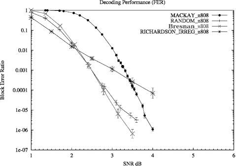
Figure 13: Block error rate performance for $N=808$ Bresnan code compared with three random like codes of the same length obtained from MacKay, Richardson and random permutations methods.

The performance of the new code is close to that of the random-edge one, with the Random code hitting an error floor around $3db$m $1e-05$. The MACKAY code performs worse than the new codes losing $0.5dB$ at $1e-06$. The Richardson code has particularly poor performance, it is possible that the code constructed is a bad representative of the ensemble of which it is part. It is known that for medium and shorter length codes the performance of the single codes varies widely from the average performance of the ensemble and from the performance of long codes for the same construction. On the other hand the situation highlights the problem of finding good random codes: creation and simulation of many codes are necessary to find a good one.

Figure 14 shows the performances comparison between $N=1048$ $R=1/2$ codes constructed with MacKay method [40], Random code [41] and a quasi-cyclic  code of this class. It can be seen that the performance of the quasi-cyclic  code is close to the one of the random one, it is slightly worse when the code meets a noise floor. The performance of the MacKay code in the $1dB-4dB$ range is worse than the quasi-cyclic  code. For low values of SNR the quasi-cyclic  code performance compares well with the random code, and both are superior to the MacKay one.

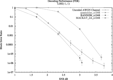
Figure 14: Block error rate performance for $N=1048$ Bresnan code compared with the a code obtained with the random permutation method and one with MacKay methods.

Even if the main interest of this thesis is on medium length codes it is interesting to evaluate the construction presented for longer codes to have an idea of how such family performs in such case, for this reason two code with $N\approx 10,000$, are presented. In Figure 15 a Bresnan code is compared with a MacKay code, it can be seen how the MacKay code has a much better defined waterfall region that make the code outperform the Bresnan code for high SNR, this could be due to low minimum distance or to the presence of trapping sets. The result is in line with what is a know fact: analytic codes do not perform as well as random codes for high length. Moreover it proves that the MacKay codes for this length start to behave as it is theoretically proved for infinite length.

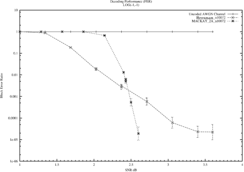
Figure 15: Block error rate performance for $N\approx 10,000$. A Bresnan quasi-cyclic  code and a MacKay code are compared.

Finally it is important to consider that for the concentration theorem [9] it is more likely that a code taken at random from the ensemble performs as well as the average performance of the ensemble for this value of $N$. It is important to observe that the construction of good random codes, such as the three confronted here, requires a consistent amount of computation, while the new codes can be obtained immediately, thanks to their simple structure.

8 Extension of the Bresnan Codes

In this section an approach to construct Bresnan-like codes with rate higher than $1/2$ is presented that maintain girth $8$.

The Bresnan codes are formed by two square blocks of circulants, the codes developed in this section are formed by three blocks. A rate of $2/3$ is achievable in such way. The method is expandable to more blocks and any rate of the type $(l-1)/l$ can be achieved.

Definition 8.1 (Rate $2/3$ Bresnan codes).

Let $\alpha,m$ be positive integers such that $\alpha>4,m\geq 3$. $\mathbb{H}_{m,\alpha}$ denotes the class of the $(m\alpha\times 3m\alpha)$ matrices of the form

$$H=\left[\begin{array}[]{ccccc|ccccc|ccccc}H^{1}_{1}&0&\ldots&0&I&H^{2}_{1}&I&0&\ldots&0&H^{3}_{1}&0&I&\ldots&0\\ I&H^{1}_{2}&0&\ldots&0&0&H^{2}_{2}&I&&\vdots&0&H^{3}_{2}&0&I&\ldots\\ 0&I&\ddots&\ddots&\vdots&\vdots&0&\ddots&\ddots&0&\vdots&0&\ddots&\ddots&\ddots\\ \vdots&&\ddots&\ddots&0&0&&\ddots&\ddots&I&\vdots&&\ddots&\ddots&0\\ 0&\ldots&0&I&H^{1}_{\alpha}&I&0&\ldots&0&H^{2}_{\alpha}&0&I&\ldots&0&H^{3}_{\alpha}\\ \end{array}\right].$$

where every $H^{c}_{i}$, with $c\in\{1,2\}$ and $i\in\{1,2,..,\alpha\}$, is an $m\times m$ binary weight-$2$ circulant matrix and $I$ is the $m\times m$ identity matrix.

To simplify the discussion the three blocks that form the $\mathbf{H}$ matrix are called $B_{1}$, $B_{2}$ and $B_{3}$ and $\mathbf{H}=[B_{1}|B_{2}|B_{3}]$. The following theorem lists all the conditions that must hold for an $\mathbf{H}$  matrix of this type to have girth exactly eight.

Theorem 8.2.

Let $m\geq 3$, $\alpha>4$ and $M\in\mathbb{H}_{m,\alpha}$. Let $g$ be the girth of the Tanner graph of $M$. Then $g=8$ if and only if all the following conditions hold:

1. for any $1\leq i\leq\alpha$ and $c\in\{1,2,3\}$

   $$s(p_{i}^{c})\not=\frac{m}{3}, s(p_{i}^{c})\not=\frac{m}{2},$$

2. for any $1\leq i\leq\alpha$ and $c,d\in\{1,2,3\}$ and $c\neq d$,

   $$\begin{array}[]{ccc}s(p_{i}^{c})\not=s(p_{i}^{d}),&s(p_{i}^{c})\not\equiv\pm 2s(p_{i}^{d}),\end{array}$$

3. for any $1\leq i\leq\alpha$,
   $\begin{aligned} \qquad s(p_{i}^{1})\pm s(p_{i}^{2})\pm s(p_{i}^{3})\not\equiv 0,\end{aligned}$

4. for any $(i,j)\in J_{\alpha}$,

   • $\epsilon(p_{i}^{1})+\epsilon(p_{j}^{2})\not\equiv 0,$

   • $\epsilon(p^{1}_{i})+\epsilon(p^{2}_{j})\not\equiv\{\pm s(p^{1}_{i}),\pm s(p^{2}_{j})\},$

   • $\epsilon(p^{1}_{i})+\epsilon(p^{2}_{j})\not\equiv\{\pm s(p^{1}_{j}),\pm s(p^{2}_{i}),\pm s(p^{3}_{i}),\pm s(p^{3}_{j})\}.$

5. for any $1\leq i\leq\alpha$,
   $\begin{aligned} \quad s(p^{1}_{i})&\not\equiv\{s(p^{1}_{i+1}),s(p^{2}_{i+1}),s(p^{3}_{i+1}),s(p^{3}_{i+2})\},\\ \quad s(p^{2}_{i})&\not\equiv\{s(p^{2}_{i+1}),s(p^{3}_{i+2})\},\\ \qquad s(p^{3}_{i})&\not\equiv\{s(p^{3}_{i+2}),s(p^{2}_{i+1})\},\end{aligned}$

6. for any $1\leq i\leq\alpha$,

   • $\epsilon(p^{1}_{i})+\epsilon(p^{1}_{i+1})+\epsilon(p^{3}_{i+2})\not\equiv 0$

   • $\epsilon(p^{2}_{i})+\epsilon(p^{2}_{i+1})-\epsilon(p^{3}_{i+1})\not\equiv 0$

   • $\epsilon(p^{1}_{i})-\epsilon(p^{2}_{i})+\epsilon(p^{3}_{i+1})\not\equiv 0$

   • $\epsilon(p^{1}_{i})-\epsilon(p^{2}_{i+2})+\epsilon(p^{3}_{i+2})\not\equiv 0$

Proof.

It is necessary to prove that the conditions listed in the statement cover all the possible cycle configurations existing for the construction presented. To prove this it is necessary to show that the configurations, regarding cycles of length $4$ and $6$ in theorem 6.1, or are not possible for this construction, or are associated with conditions listed in the statement.

• Configurations 1.1 and 2.1 in theorem 6.1 are evidently associated with the conditions in point 1.

• Configurations 1.2 and 2.2 are covered by the conditions in point 2.

• Point 3 considers configuration 2.3 in theorem 6.1.

• Configuration 1.3 is considered by condition in point 4.1. Note that due to the position of the diagonal of identities in $B_{3}$ such configuration can exist only between $B_{1}$ and $B_{2}$.

• Configuration 1.4 cannot exist in the proposed class thanks to the position of the identities diagonals. There cannot be any couple of columns that have $H$ and $I$ sub-matrices in the same two rows.

• Configuration 2.4 in considered by the conditions in point 5. In fact every $H$ sub-matrix has three $I$ sub-matrices lying in the same row and one in the same column. Hence for every $H$ sub-matrix six possible cycles of the type 2.4 can exist, three formed by the three identities in the same row and three formed by the identity in the same column and the three $H$ sub-matrices lying in the row of such $I$.
  The conditions for cycles to existing in such configuration are:

  $$s(p^{1}_{i}) \equiv\{s(p^{1}_{i-1}),s(p^{2}_{i+1}),s(p^{3}_{i+2})\},$$

  $$s(p^{1}_{i}) \equiv\{s(p^{1}_{i+1}),s(p^{2}_{i+1}),s(p^{3}_{i+1})\},$$

  $$s(p^{2}_{i}) \equiv\{s(p^{2}_{i-1}),s(p^{2}_{i+1}),s(p^{3}_{i+2})\},$$

  $$s(p^{2}_{i}) \equiv\{s(p^{2}_{i-1}),s(p^{2}_{i-1}),s(p^{3}_{i-2})\},$$

  $$s(p^{3}_{i}) \equiv\{s(p^{3}_{i+2}),s(p^{1}_{i-1}),s(p^{2}_{i+1})\},$$

  $$s(p^{3}_{i}) \equiv\{s(p^{3}_{i-2}),s(p^{1}_{i-2}),s(p^{2}_{i-2})\},$$

  Eliminating from the list above the conditions that are equivalent the set of conditions in point 5 is obtained.

• Configurations 2.5 cannot exist for the same reason discussed for configuration 1.4, the same is true for configurations 2.7 and 2.9 of theorem 6.1.

• Cycles from configuration 2.6 can exist only between sub-matrices in $B_{1}$ and sub-matrices in $B_{2}$ . In fact the position of the diagonal of identities in $B_{3}$ does not allow any of the columns in the third block to overlap in two positions with any of the other columns. Conditions in point 4.2 evidently cover all the possible cycles of this type.

• For the same reason of the previous point, configuration 2.8 can exist only when the $\left|\begin{smallmatrix}H^{2}-2&I\\ I&H^{3}-2\\ \end{smallmatrix}\right|$ columns are in $B_{1}$ and $B_{2}$. The remaining column can be in any of the three blocks, the relative cycles are avoided by the conditions in point 4.3.

• Cycles from configurations 2.10 and 2.11 are associated to conditions in point 6. To prove this it is necessary to show that the conditions listed in point 6 consider all possible cycles that can arise from the two configurations.

  Both configurations require that the distance from an $H$ sub-matrix and the identity in the same column is the sum of the distances from the other two $H$ sub-matrices and relative identities. It is evident from the position of the identities diagonals that such case is possible only if one column lies in $B_{3}$ and the other two columns do not. If the other columns both lie in $B_{1}$ it is only a matter of connecting the sub-matrices to see that the resulting cycle is part of configuration 2.11 and it is not allowed by the condition 6.1. If the other columns both lie in $B_{2}$ it is only a matter of connecting the sub-matrices to see that the resulting cycle is part of configuration 2.10 and it is not allowed by the condition 6.2. If one of the remaining column lies in $B_{1}$ and the other in $B_{2}$ there are two possibilities to form a cycle, both corresponding to configuration 2.10. The fist case has the $H$ sub-matrices in $B_{1}$ and $B_{2}$ lying in the same d.r., the second case has the $H$ sub-matrices in $B_{2}$ and $B_{3}$ lying in the same d.r. The resulting cycles are avoided by conditions 6.3 and 6.4 respectively.

  Note that if the two $H$ sub-matrices in $B_{1}$ and $B_{3}$ lie in the same d.r. is not possible to form a cycle due to the position of the identities diagonals

It has been proved that all the possible cycles that can exist in the $\mathbf{H}$ matrix for this class of codes is avoided by one of the condition listed. ∎

The performance of such class of codes is presented next. Figure 16 shows the comparison between a code from the class of quasi-cyclic  codes presented versus a random code and a MacKay code obtained from [42], the codes have length $N\approx 200$. The codes have similar length and rate, the MacKay code is slightly longer but has higher rate $R\approx 0.7$. It can be seen how the quasi-cyclic  code and MacKay code perform closely and slightly better than the random code.

The comparison of the same families of codes for $N\approx 1,000$ is presented in Figure 17. The codes have similar length and rate, the MacKay code is slightly longer but has higher rate $R\approx 0.85$. For such length the proposed quasi-cyclic  code outperforms both the random code and the MacKay code. In particular the random code seems to hit an early error floor and the MacKay code perform few tens of dB worse for all the SNR range considered.

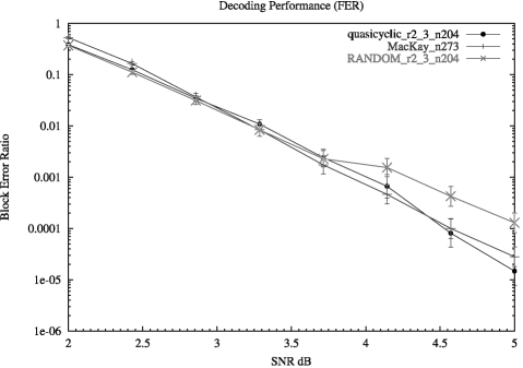
Figure 16: Block error rate performances comparison of a regular quasi-cyclic  codes with $R=2/3$ versus a MacKay codes and a random permutation codes of similar rate and length $N\approx 200$

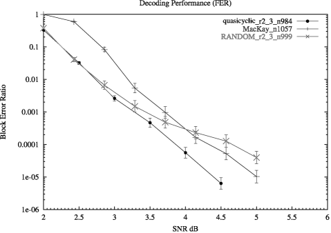
Figure 17: Block error rate performances comparison of a regular quasi-cyclic  codes versus a random constructed code and a MacKay code, $N\approx 1,000$. All codes have similar rate.

Finally Figure 18 presents the comparison of a quasi-cyclic  code with a random code for $N=2457$. Unfortunately it has not been possible to obtain a MacKay code with such rate and length due to failure of the search carried out. The random code performs slightly better than thequasi-cyclic  code for low SNR but it is affected by early error floor that makes its performance poor at higher SNR. In contrast the quasi-cyclic  code does not show the presence of any early error floor.

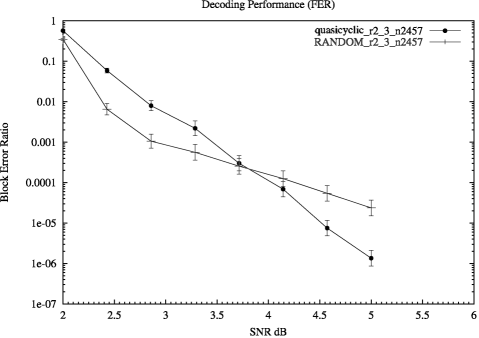
Figure 18: Block error rate performances comparison of a regular quasi-cyclic  codes versus a random constructed code with same rate and length $N\approx 2,000$

It can be concluded that the construction proposed is a valid alternative to random like codes for high rate. The quasi-cyclic  codes, for the dimensions considered, perform at least as well as other constructions but offer the advantage of reduced complexity and minimize memory requirement. Those are important aspects for many applications where high rate codes are used.

9 Two families of quasi-cyclic  codes with girth 10

In this section two families of quasi-cyclic  LDPC codes with girth at least 10 and rate $1/2$ are presented. The first construction is a $(2,4)$-regular codes, the second a $(3,6)$-regular codes. The constructions are based on the idea of using blocks of circulants to compose the $\mathbf{H}$  matrix. The circulants lie in the diagonals of the block, this help to detect the possible configurations arising and can be exploited to reduce hardware complexity of the decoding algorithm (see [38]).

9.1 Regular $(2,4)$

This family of codes has been studied first because its structure drastically reduce the number of conditions necessary to ensure high girth.

Definition 9.1 ( $(2,4)$-regular quasi-cyclic  codes girth 10).

Let $\alpha,m$ be positive integers such that $\alpha>4,m\geq 3$. Notation $\mathbb{C}_{m,\alpha}$ denotes the class of the $(m\alpha\times 2m\alpha)$ matrices of the form

$$\mathbf{H}=\left[B_{1}\,|\,B_{2}\right]$$

where

$$B_{1}=\left[\begin{array}[]{ccccc}H_{0}&0&\ldots&0&0\\ 0&H_{1}&0&\ldots&0\\ 0&0&\ddots&\ddots&\vdots\\ \vdots&&\ddots&\ddots&0\\ 0&\ldots&0&0&H_{\alpha-1}\\ \end{array}\right]$$

and

$$B_{2}=\left[\begin{array}[]{ccccc}I&0&\ldots&J_{0}&0\\ 0&I&0&\ldots&J_{1}\\ J_{2}&0&\ddots&\ddots&\vdots\\ \vdots&&\ddots&\ddots&0\\ 0&\ldots&J_{\alpha-1}&0&I\\ \end{array}\right].$$

Where every $H_{i}$, with $i\in\{0,1,..,\alpha-1\}$, is an $m\times m$ binary weight-$2$ circulant matrix, $J_{i}$ are binary weight-$1$ circulant matrices and $I$ is the $m\times m$ identity matrix.

Reducing the theorems studied in section 5 for this class of matrices is a long task. This can be eased by considering that some of the cycle configurations listed in theorems 5.3, 5.7, 5.16 can exist only if the distance from the main diagonal and the diagonal of $J$’s in $B_{2}$ is a particular value. Such distance is called $\delta$.

The following theorem lists all the conditions that must hold for an $\mathbf{H}$  matrix of this class to have girth at least $10$.

Theorem 9.2.

Let $m\geq 3$, $\alpha>4$ and $\mathbf{H}$ $\in\mathbb{C}_{m,\alpha}$. Let $g$ be the girth of the Tanner graph of $\mathbf{H}$ . Then $g\geq 10$ if and only if all the following conditions hold for any $0\leq i\leq\alpha-1$.

1. $$\begin{array}[]{ccc}s(p_{i})\not=\frac{m}{2},&s(p_{i})\not=\frac{m}{3},&s(p_{i})\not=\frac{m}{4},\end{array}$$

2. $$s(p_{i})\not=s(p_{i+\delta}),$$

3. $$\mbox{or}\quad\delta\not=\alpha/2,\quad\mbox{or}\quad\left\{\begin{aligned} &3.1\quad\epsilon(p_{i})^{J}+\epsilon(p_{i+\delta})^{J}&\not\equiv&0,&\mbox{and}\\ &3.2\quad\epsilon(p_{i})^{J}+\epsilon(p_{i+\delta})^{J}&\not\equiv&\pm s(p_{i})&\mbox{and}\\ &3.3\quad\epsilon(p_{i})^{J}+\epsilon(p_{i+\delta})^{J}&\not\equiv&\pm s(p_{i+\delta})&\mbox{and}\\ &3.4\quad 2\epsilon(p_{i})^{J}+2\epsilon(p_{i+\delta})^{J}&\not\equiv&0,&\mbox{and}\\ &3.5\quad\epsilon(p_{i})^{J}+\epsilon(p_{i+\delta})^{J}&\not\equiv&\pm 2s(p_{i})&\mbox{and}\\ &3.6\quad\epsilon(p_{i})^{J}+\epsilon(p_{i+\delta})^{J}&\not\equiv&\pm 2s(p_{i+\delta})&\mbox{and}\\ &3.7\quad\epsilon(p_{i})^{J}+\epsilon(p_{i+\delta})^{J}&\not\equiv&\pm s(p_{i})\pm s(p_{i+\delta})\\ \end{aligned}\right.$$

4. $$\mbox{or}\quad\delta\not=\pm\alpha/3,\quad\mbox{or}\quad\left\{\begin{aligned} &4.1\quad\epsilon(p_{i})+\epsilon(p_{i+\delta})+\epsilon(p_{i+2\delta})\not\equiv 0&\mbox{and}\\ &4.2\quad\epsilon(p_{i})+\epsilon(p_{i+\delta})+\epsilon(p_{i+2\delta})\not\equiv\pm s(p_{i})\\ \end{aligned}\right.$$

5. $$\mbox{or}\quad\delta\not=\pm\alpha/4,\quad\mbox{or}\quad\epsilon(p_{i})+\epsilon(p_{i+\delta})+\epsilon(p_{i+2\delta})+\epsilon(p_{i+3\delta})+\epsilon(p_{i+4\delta})\not\equiv 0$$

Where the index operations are modulo $alpha$.

Proof.

It is necessary to prove that the conditions listed cover all the possible cycle configurations existing in such class of codes. To prove this it is necessary to show that the configurations listed in theorems 5.3, 5.7 and 5.16 are not possible for this construction or are associated with a condition listed in the statement. First the configurations that can have $4$-cycles, listed in theorem 5.3, are considered.

• Configuration 1 is associated with the first condition in point 1.

• Configuration 2 cannot exist because there cannot be two $H$ sub-matrices in the same row or column.

• Configuration 3 can exist in this construction only if $\delta=\alpha/2$. In any other case there cannot be four sub-matrices lying in two columns and two rows. If $\delta=\alpha/2$ condition 3.1 assures that the cycle cannot exist.

The configurations that can have $6$-cycles, listed in theorem 5.7, are considered next.

• Configuration 1 is associated with the second condition in point 1.

• Configurations 2 and 3 cannot exist because there cannot be two $H$ sub-matrices in the same row or column.

• Configurations 4 and 5 cannot exist because for this construction every $H$ sub-matrix lies alone in a column.

• For the same reason discusses for configuration 3 of theorem 5.3, configuration 6 can exist in this construction only if $\delta=\alpha/2$. If $\delta=\alpha/2$ conditions 3.2 and 3.3 assure that the cycle cannot exist.

• Configurations 7 requires that the distance from two sub-matrices in the same column is the sum of the two other such distances for the remaining d.c.’s in the configuration. It is evident that all the columns must lie in $B_{2}$ since in $B_{1}$ there is only one sub-matrix in each column. Moreover such situation exists only if $\delta=\pm\alpha/3$. If $\delta=\pm\alpha/3$ conditions 4.1 assures that the cycle cannot exist. To determine the sign of the terms in the condition it is sufficient to consider that there cannot be two $J$’s in the same column. Hence the $J$’s take alternate positions in the cycle configuration hence they all have the same sign.

The configurations that can have $8$-cycles, listed in theorem 5.16 are considered next.

• Configuration 1 is associated with the third condition in point 1.

• Configurations 2, 3, 4, 7, 12 and 15 cannot exist because for this construction every $H$ sub-matrix lies alone in a column.

• For the same reason discussed for configuration 3 of theorem 5.3, configuration 5 can exist in this construction only if $\delta=\alpha/2$. If $\delta=\alpha/2$ conditions 3.4 assures that the cycles cannot exist.

• For the same reason of previous point, configuration 6 can exist in this construction only if $\delta=\alpha/2$. If $\delta=\alpha/2$ conditions 3.5 and 3.6 assure that the cycles cannot exist.

• Configuration 8 cannot exist because the structure of the $\mathbf{H}$ does not allow to have $6$ sub-matrices lying in two rows and three columns.

• Configuration 9 is evidently associated with condition 2.

• Configuration 10 can exist only with $\delta=\alpha/2$ for the same reason discussed in previous cases. If $\delta=\alpha/2$ conditions 3.7 assures that the cycles cannot exist.

• Configuration 11 cannot exist because the structure of the $\mathbf{H}$ does not allow to have $8$ sub-matrices lying in two rows and four columns.

• Configuration 13 cannot exist because it implies the existence of three non zero sub-matrices in the same column or the existence of a column with an $H$ and one identity, both cases are not possible due to the particular structure of the $\mathbf{H}$ matrix.

• Configuration 14 cannot exist because it implies to have three non zero sub-matrices in the same column that is not possible due to the particular structure of the $\mathbf{H}$ matrix.

• Configuration 16 cannot exist because it implies to have four non zero sub-matrices in the same column or row that is not possible due to the particular structure of the $\mathbf{H}$ matrix.

• Configuration 17 requires that the distance from an two sub-matrices in the same column is the sum of the two other such distances for the remaining d.c.’s in the configuration. It is evident that the columns not containing $H$ must lie in $B_{2}$. Moreover such situation exist only if $\delta=\pm\alpha/3$. If $\delta=\pm\alpha/3$ conditions 4.2 assures that the cycle cannot exist. The same reasoning applied to configuration 7 of theorem 5.7 can be used to explain the signs of the terms of the condition.

• Configurations 18 requires that the distance from the two sub-matrices in the same column is the sum of the three other such distances for the remaining d.c.’s in the configuration. It is evident that all the columns must lie in $B_{2}$. Moreover such situation exist only if $\delta=\pm\alpha/4$. If $\delta=\pm\alpha/4$ conditions 5 assures that the cycles cannot exist.

It has been proved that all the possible cycles that can exist in the $\mathbf{H}$ matrix for this class of codes is avoided by one of the condition listed. ∎

Aside from the degenerative cases where $\delta=\alpha/2$, $\delta=\alpha/3$ and $\delta=\alpha/4$ the conditions to check are extremely simple. Even in the degenerative cases the list of conditions is quite short. Thanks to this, finding exponents and conditions that allows girth $10$ is an easy task. Following the performances of three of such codes are presented. The codes have been obtained avoiding the degenerative cases of $\delta$ and imposing the conditions on the separations.

In Figure 19 the block error ratio versus noise performance graph of a small code ($N=810$) from this family can be seen. The code is compared with a random code. Both codes have same length and are $(2,4)$-regular. The random codes has been obtained with a optimal permutations method and has a girth of $14$ and an average girth of $15.7$, the quasi-cyclic  codes has girth $10$. In the same figure the quasi-cyclic  code is compared also with a more advanced Progressive Edge Grow (PEG) code from [43, 44]. The code is $(2,7)$-regular. It can be seen how this code performs as well as the random code and compares evenly with a carefully constructed code, this is a good result for such class of codes.

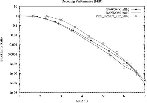
Figure 19: Block error rate performances comparison of a quasi-cyclic  code compared with a random code and a PEG code with $N\approx 800$

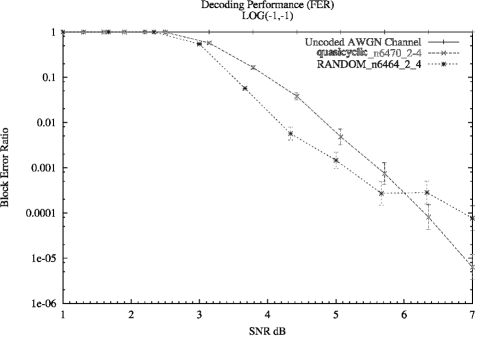
Figure 20: Block error rate performances comparison of a quasi-cyclic  code compared with a random code. Both codes are $(2,4)$-regular with $N\approx 6,500$

Figure 20 presents a comparison of a quasi-cyclic  code from this family versus a random code in the case of longer codes. Both the codes have $N\approx 6,500$. It can be seen how the performance of the quasi-cyclic  code with girth 10 do not hit an error floor as soon as the random code. The random code has average girth of $20.37$ but girth of only $6$.

Regular $(2,4)$-LDPC codes are not often used in practice due to their poor performances. As an example of this a comparison between a $(3,6)$-regular Gallagher code and the PEG code is presented in Figure 21 It can be seen how the $(3,6)$- regular code has up to 5db gain when compared with $(2,4)$-regular codes both random and quasi-cyclic . For this reason the interest is on build $(3,6)$-regular quasi-cyclic  LDPC codes with girth ten.

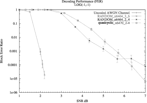
Figure 21: Block error rate performances comparison of a $(2,4)$-regular quasi-cyclic  codes versus a $(3,6)$-regular code $N\approx 800$

9.2 Regular $(3,6)$

The construction presented here is the result of few considerations. Lemma 5.15 shows how any quasi-cyclic  LDPC code with girth at least $10$ cannot exist if two weight-$2$ circulants lie in the same row or column. For this reason all weight-2 circulants are placed in the main diagonal of $B_{1}$. To keep the column weight equal to three it is necessary to insert another weight-1 circulant for each column and this is done inserting another diagonal of identities. The second block $B_{2}$ cannot contain weight two circulants hence any row and column must contain three weight-$1$ circulants to form a $(3,6)$-regular code. Aiming to maintain some regularity to allow reduced hardware complexity of the decoding algorithm, the circulant matrices have been disposed in three diagonals. To simplify the number and complexity of the checks necessary to guarantee girth $10$ identity matrices, as special case of weight-$1$ circulant matrices, have been used where possible.The resulting family of codes is the following.

Definition 9.3 ($(3,6)$-regular quasi-cyclic  code).

Let $\alpha,m$ be positive integers such that $\alpha>4,m\geq 3$. Notation $\mathbb{D}_{m,\alpha}$ denotes the class of the $(m\alpha\times m\alpha)$ matrices of the form

$$\mathbf{H}=\left[B_{1}\,|\,B_{2}\right]$$

where

$$B_{1}=\left[\begin{array}[]{ccccc}H_{0}&0&\ldots&0&I\\ I&H_{1}&0&\ldots&0\\ 0&I&\ddots&\ddots&\vdots\\ \vdots&&\ddots&\ddots&0\\ 0&\ldots&0&I&H_{\alpha-1}\\ \end{array}\right]$$

and

$$B_{2}=\left[\begin{array}[]{cccccccccccc}J_{0}&0&\ldots&0&I&0&\ldots&0&I&0&\ldots&0\\ 0&J_{1}&0&\ldots&0&I&0&\ldots&0&I&\ldots&\vdots\\ \vdots&&\ddots&&&&\ddots&&&&\ddots&0\\ \vdots&&&\ddots&&&&\ddots&&&&I\\ I&0&&&\ddots&&&&\ddots&&&0\\ 0&\ddots&&&&\ddots&&&&\ddots&&0\\ \vdots&&\ddots&&&&\ddots&&&&\ddots&0\\ &&&\ddots&&&&\ddots&&&&I\\ I&&&&\ddots&&&&\ddots&&&0\\ 0&\ddots&&&&\ddots&&&&\ddots&&\vdots\\ \vdots&&\ddots&&&&\ddots&&&&\ddots&\\ 0&&&I&\ldots&&&I&\ldots&&&J_{\alpha-1}\\ \end{array}\right].$$

where every $H_{i}$, with $i\in\{0,1,..,\alpha-1\}$, is an $m\times m$ binary weight-$2$ circulant matrix and $I$ is the $m\times m$ identity matrix, and $J_{i}$ are weight-$1$ circulant matrices.

Some of the cycle configurations listed in theorems 5.3, 5.7 and 5.16 exist only if the distance from the main diagonal and the diagonals of identities in $B_{2}$ take particular values. Such distances are called $\delta_{2},\delta_{3}$, and for simplicity the notation $\delta_{3}-\delta_{2}$ is called $\delta_{32}$. Such values can be seen in Figure 22. Moreover the position of the diagonal of identities in $B_{1}$ is called $\delta_{1}$. For the construction presented here $\delta_{1}=\alpha-1$.

Note that it is not possible to substitute the diagonal of $J$’s with identities. In fact in such case $6$-cycle configurations will always arise independently from the positions of the diagonals. The existence of this configurations carry a parallel with the existence of $6$-cycles on a weight-$3$ circulant matrix [33]. A graphical representation of such case is given in Figure 22. It can be seen that the particular $6$-cycle exists if $\delta_{2}+\delta_{32}=\delta_{3}$ but $\delta_{2}+\delta_{3}-\delta_{2}=\delta_{3}$ hence the condition is always satisfied and the cycle exists independently from the values of the deltas. If all the matrix involved in the cycle are identities it is not possible to avoid such cycle. Setting the main diagonal to contain $J$’s, and not identities, it is possible to avoid such cycle by imposing proper conditions on the exponents.

\psfrag{d2}{$\delta_{2}$}\psfrag{d3}{$\delta_{3}$}\psfrag{d32}{$\delta_{32}$}\includegraphics[angle={0},width=346.89731pt]{./deltas.eps}

Figure 22: Example of configuration existing independently from the values of the deltas

A new class of matrices is presented next. The matrices are part of the previous class but some limitations on the position of the diagonals of identities are added. Such limitations on the values of deltas are not strictly necessary but help to reduce the number of possible configurations, and so the complexity of the conditions to check.

Definition 9.4 ($(3,6)$-regular quasi-cyclic  code girth 10).

Let $\mathbb{E}_{m,\alpha}$ denotes the class of the $(m\alpha\times m\alpha)$ matrices in $\mathbb{D}_{m,\alpha}$ that satisfy the following conditions on the distances of the diagonals.

(46) $$\begin{array}[]{lll}1&\quad\delta_{x}\not=\alpha/2,\;\delta_{x}\not=\pm\alpha/3,\;\delta_{x}\not=\pm\alpha/4&\mbox{ where }x\in\{2,3,32\}\\ 2&\quad\delta_{x}\not=\pm\delta_{y},&\mbox{ where }x,y\in\{1,2,3,32\}\;\mbox{and}\;x\neq y\\ 3&\quad\delta_{x}\pm\delta_{y}\pm\delta_{z}\not=0,&\mbox{ where }x,y,z\in\{2,3,32\}\\ 4&\quad\delta_{x}\pm\delta_{y}\pm\delta_{z}\pm\delta_{w}\not=0,&\mbox{ where }x,y,z,w\in\{1,2,3,32\}\\ \end{array}$$

Once those conditions (on the deltas) are verified it is possible to apply the theorems studied in section 5 to obtain the set of conditions (on the circulants) that assure girth at least 10.

Theorem 9.5.

Let $m\geq 3$, $\alpha\geq 4$ and $\mathbf{H}$ $\in{\mathbb{E}_{m,\alpha}}$. Let $g$ be the girth of the Tanner graph of $\mathbf{H}$ . Then $g\geq 10$ if and only if all the following conditions hold for any $0\leq i\leq\alpha-1$ :

1. $$\begin{array}[]{ccc}s(p_{i})\not=\frac{m}{2},&s(p_{i})\not=\frac{m}{3},&s(p_{i})\not=\frac{m}{4},\end{array}$$

2.       

   • $s(p_{i})\not\equiv s(p_{i+\delta_{1}}),$

   • $s(p_{i})\not\equiv\pm 2s(p_{i+\delta_{1}}),$

   • $s(p_{i+\delta_{1}})\not\equiv\pm 2s(p_{i}),$

3. $$\begin{array}[]{cc}s(p_{i})\not\equiv s(p_{i+\delta_{x}}),&\mbox{ where }x\in\{2,3,32\}\\ \end{array}$$

4.                   

   • $\epsilon(p_{i})^{J}-\epsilon(p_{i\pm\delta_{32}})^{J}\not\equiv 0,$

   • $\epsilon(p_{i})^{J}-\epsilon(p_{i+\pm\delta_{32}})^{J}\not\equiv\pm s(p_{i}),$

5.                   

   • $\epsilon(p_{i})^{H}-\epsilon(p_{i\delta_{32}})^{H}\not\equiv 0,$

   • $\epsilon(p_{i})^{H}-\epsilon(p_{i-\delta_{x}})^{H}+\epsilon(p_{i+1})^{J}-\epsilon(p_{i})^{J}\not\equiv 0\qquad\mbox{ where }x\in\{2,3\}$

Proof.

It is necessary to prove that the conditions listed cover all the possible cycle configurations existing in such class of codes. To prove this it is necessary to show that the configurations listed in theorems 5.3, 5.7 and 5.16, or are not possible for this construction, or are associated with a condition listed in the statement. First the configurations that can have $4$-cycles, listed in theorem 5.3 are considered.

• Configuration 1 is associated with the first condition in point 1.

• Configuration 2 cannot exist because there cannot be two $H$ sub-matrices in the same row or column.

• Configuration 3 cannot exist in this construction and with the conditions imposed on the deltas. In fact such configuration can exist only if there are four sub-matrices lying in two column and two rows. This can happen only if two deltas are equals modulo alpha, or if one of the delta is equal to $\alpha/2$. These cases are not allowed by conditions 1 and 2 in definition 9.4 hence the cycle configuration cannot exist.

The configurations that can have $6$-cycles, listed in theorem 5.7 are considered next.

• Configuration 1 is associated with the second condition in point 1.

• Configurations 2 and 3 cannot exist because there cannot be two $H$ sub-matrices in the same row or column.

• Configuration 4 contains two $C$ sub-matrices in the two d.c. hence both the columns must be in the $B_{1}$. Every $H$ sub-matrix can form a cycle only with the row above and below itself. All this cases are considered by condition 2.1. The remaining sub-matrix in the configuration is an identity hence the two exponent terms are not present in the final condition.

• Configurations 5 and 6 cannot exist for the same reason discussed for configuration 3 of theorem 5.3.

• Configurations 7 requires that the distance from two sub-matrices in the same column is the sum of the two other such distances for the remaining d.c.’s in the configuration. This is not allowed by condition 3 in definition 9.4 with the exception of the case depicted in Figure 22. Such cycles are avoided by condition 4.1.

The configurations that can have $8$-cycles, listed in theorem 5.16 are considered next.

• Configuration 1 is associated with the third condition in point 1.

• Configurations 2, 4, 5, 6, 7, 8, 10, 11, 13, 14, 15 and 16 cannot exist for the same reason discussed for configuration 3 of theorem 5.3 .

• The same reasoning done for configuration 4 of theorem 5.7 applies to configuration 3 and all the possible resulting cycles are avoided by conditions 2.2 and 2.3.

• Configuration 9 contains two $C$ sub-matrices in the two d.c. hence both the columns must be in $B_{1}$. The remaining column contains two $J$ sub-matrices hence it must lie $B_{2}$. The sub-matrices in the column in $B_{2}$ are spaced at distance $\delta_{x}$ with $x\in\{2,3,32\}$ hence all the possible cycles are considered by condition 3.

• Configuration 12 requires that the distance from two sub-matrices in the same column is the sum of the two other such distances for the remaining d.c.’s in the configuration. This is not allowed by condition 3 in definition 9.4. Note that the presence of a weight-$2$ circulant forces one d.c. to be in $B_{1}$ hence the case depicted in Figure 22 does not exist here.

• Following the same reasoning done for configuration  7 of theorem 5.7. Configuration  17 exists only if the three columns lying in B2 have the configuration depicted in Figure 22 and the last column lies in B1. Such cycles are avoided by condition 4.2.

• Configuration 18 is associated to conditions in point 5. To prove this it is necessary to show that the conditions listed in point 5 consider all possible cycles that can arise from the configuration.

  The configuration requires that the distance of two sub-matrices in the same column is the sum of the three other such distances for the remaining d.c.’s in the configuration. Such configurations are not possible thanks to condition 4 in definition 9.4. A particular case remains to be considered. If two columns of the cycle configuration lie in $B_{1}$ and two in $B_{2}$ then the existence of this configurations carry a parallel with the existence of $8$-cycles on two weight-$2$ circulants in the same row or column (Figure 12). It has been proved in lemma 5.15 that such cycle exists independently from the value of the separations. In this case the delta’s take the part of the separation, hence the cycle configuration exists independently from the value of delta’s. But $B_{2}$ has three diagonals so three different cycles can exist, and such cycles are avoided by the three conditions in point 5.

  To better understand this passage consider that the two cycle columns in $B_{1}$ contain an identity and an $H$ sub-matrix each, hence exponents of two $H$ sub-matrices must be part of the condition. From Figure 12 it can be seen that the cycle exists only if both the cycle columns in $B_{2}$ contain two sub-matrices appertaining to the same two diagonals. There are three possibilities: one sub-matrix is in the second diagonal and one in the main diagonal, one sub-matrix is in the third diagonal and one in the main diagonal and finally one sub-matrices in the second diagonal and one in the third diagonal. The first two cases lead to condition 5.2 the third to condition 5.1.

It has been proved that all the possible cycles that can exist in the $\mathbf{H}$ matrix for this class of codes is avoided by one of the condition listed. ∎

Following the performances of codes of this family for different lengths are presented.

Figure 23 shows the performance of a medium length quasi-cyclic  code when compared with a random generated code. Both codes are $(3,6)$-regular codes of dimension $N=2,294$. It can be seen how the quasi-cyclic  codes from this family performs really close to the random code, but it seems that the quasi-cyclic  codes hit an error floor at $1e-09$ BER.

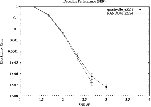
Figure 23: Block error rate performances of a girth 10 quasi-cyclic  code compared with a random generated codes. Both codes are $(3,6)$-regular with $N=2,294$

Even if out of the boundaries of the range of codes that are the main focus of this thesis the comparison of quasi-cyclic  codes with random codes using longer codes is presented next for completeness. Figure 24 and 25 present such a comparison. Figure 24 shows the performances of two $(3,6)$-regular codes with $N\approx 6,500$ and Figure 25 shows the performances of two $(3,6)$-regular codes with $N\approx 19,500$ It can be seen the quasi-cyclic  codes are quite close to the random codes. With $N\approx 6,500$ only $0.1$db, at $1e-09$, divides the two codes, with $N\approx 19,500$ the difference increased but remain under the $0.5$db, at $1e-05$, that is a considerable achievement for algebraic codes of this length.

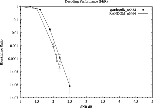
Figure 24: Block error rate performances comparison of a quasi-cyclic  code compared with a random code. Both codes are $(3,6)$-regular with $N\approx 6,500$

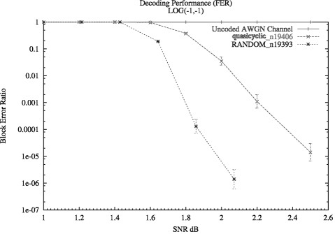
Figure 25: Block error rate performances comparison of a quasi-cyclic  code compared with a random code. Both codes are $(3,6)$-regular with $N\approx 19,500$

10 Conclusions anf future work

In this contribution a study on the presence of cycles on the quasi-cyclic  LDPC codes has been presented. The aim of the study is to identify the configurations of circulant matrices that allow cycles of a given length to exist. Once all such configurations are known it is possible to associate to each of them a condition, on the exponents and separations of the circulants involved in the cycle, that must be satisfied for the cycle to exist. The collection of these conditions gives a way to construct quasi-cyclic  codes without undesired cycle by ensuring that all the conditions are not satisfied. The chapter started with a novel definition of cycles in a matrix, opposed to the normal definition that is given on graph. Such a definition is used to prove the “isolation” (lemma 3.10), the lemma is extensively used in the search of which configurations are valid and can contain cycles. The configurations that allows cycle of length less then $10$ are found first for the generic case of a matrix that can be partitioned in sub-matrices, then in the case of the matrices for quasi-cyclic  codes. Our approach is not restricted to circulant matrices of weight one as is commonly done in literature but considers also circulant matrix of weight-$2$ (weight-$3$ circulant matrices are of no interest for this search because they have internal $6$-cycles). The set of conditions for the generic case is found and then the conditions are applied for various particular constructions. The first class of quasi-cyclic  codes studied are the Bresnan Codes [36], several aspects of these codes are studied and their performances presented. Such class is then extended for higher rate codes. Finally two new structures and the relative set of conditions that guarantee girth at least $10$ are developed and their performances presented. The contribution of this work is not only the four classes of quasi-cyclic  codes with high girth but mainly the creation of the list of conditions that every quasi-cyclic  codes (of any possible construction method) must satisfy to have a given girth. This not only covers all the existing cases but can be used when constructing new structures for quasi-cyclic  codes to easily identify where the cycles can exist and how to avoid them.

The methodology presented in this thesis could be used to expand the understanding of quasi-cyclic  codes. It would be possible to continue the search of codes with high girth and look for the conditions that guarantee girth twelve but, in the authors opinion, such work would be long, tedious and would carry little benefit. In fact, other parameters of the code, such as the minimum distance, the diameter, the minimum stopping set and others, will became dominant and prevent improvement in the performance of the code. Of more interest would be to study if the methodology presented could be applied to the problem of finding codes with good diameter value. It could be possible to develop a set of conditions that ensures the diameter to be a certain value. The study of how these rules intersect with the girth conditions could lead to classes of codes that can achieve given girth and diameter and offer a good balance between the two.

Appendix

Proof of theorem 3.16

Theorem 10.1 (3.16).

Let $B\in\mathcal{M}_{m,\alpha,\beta,\gamma}$.

The only possible $8$-cycle configurations are as follows (1)-presentations):

1. $(1,1)$,

   $$\left|8\right|,$$

2. $(1,2)$,
   

   $$\begin{array}[]{cc}2.1\left|\begin{array}[]{cc}6&2\\ \end{array}\right|,&2.2\left|\begin{array}[]{cc}4&4\\ \end{array}\right|,\end{array}$$

3. $(1,3)$,

   $$\left|\begin{array}[]{ccc}4&2&2\\ \end{array}\right|,$$

4. $(1,4)$,

   $$\left|\begin{array}[]{cccc}2&2&2&2\\ \end{array}\right|,$$

5. $(2,2)$,
   

   $$\begin{array}[]{ccc}5.1\par\left|\begin{array}[]{cc}5&1\\ 1&1\\ \end{array}\right|,&5.2\par\left|\begin{array}[]{cc}4&2\\ 2&0\\ \end{array}\right|,&5.3\par\left|\begin{array}[]{cc}4&2\\ 0&2\\ \end{array}\right|,\\ \\ 5.4\left|\begin{array}[]{cc}3&1\\ 3&1\\ \end{array}\right|,&5.5\left|\begin{array}[]{cc}3&1\\ 1&3\\ \end{array}\right|,&5.6\left|\begin{array}[]{cc}2&2\\ 2&2\\ \end{array}\right|,\par\end{array}$$

6. $(2,3)$,
   

   $$\begin{array}[]{ccc}6.1\left|\begin{array}[]{ccc}4&1&1\\ 0&1&1\\ \end{array}\right|,&6.2\left|\begin{array}[]{ccc}3&2&1\\ 1&0&1\\ \end{array}\right|,&6.3\left|\begin{array}[]{ccc}3&1&0\\ 1&1&2\\ \end{array}\right|,\\ \\ 6.4\left|\begin{array}[]{ccc}2&2&2\\ 2&0&0\\ \end{array}\right|,&6.5\left|\begin{array}[]{ccc}2&1&1\\ 2&1&1\\ \end{array}\right|,&6.6\left|\begin{array}[]{ccc}2&2&0\\ 2&0&2\\ \end{array}\right|,\end{array}$$

7. $(2,4)$,
   

   $$\begin{array}[]{ccc}7.1\left|\begin{array}[]{cccc}2&2&1&1\\ 0&0&1&1\\ \end{array}\right|,&7.2\left|\begin{array}[]{cccc}2&1&1&0\\ 0&1&1&2\\ \end{array}\right|,&7.3\par\left|\begin{array}[]{cccc}1&1&1&1\\ 1&1&1&1\\ \end{array}\right|,\end{array}$$

8. $(3,3)$,
   

   $$\begin{array}[]{cccc}8.1\left|\begin{array}[]{ccc}3&1&0\\ 1&0&1\\ 0&1&1\\ \end{array}\right|,&8.2\left|\begin{array}[]{ccc}2&1&1\\ 2&0&0\\ 0&1&1\\ \end{array}\right|,&8.3\left|\begin{array}[]{ccc}2&1&1\\ 1&1&0\\ 1&0&1\\ \end{array}\right|,&8.4\left|\begin{array}[]{ccc}2&0&0\\ 1&1&0\\ 1&1&2\\ \end{array}\right|.\end{array}$$

9. $(3,4)$,
   

   $$\begin{array}[]{cc}9.1\left|\begin{array}[]{cccc}2&1&1&0\\ 0&1&0&1\\ 0&0&1&1\\ \end{array}\right|,&9.2,\left|\begin{array}[]{cccc}1&1&1&1\\ 1&1&0&0\\ 0&0&1&1\\ \end{array}\right|,\end{array}$$

10. $(4,4)$,

    $$\left|\begin{array}[]{cccc}1&1&0&0\\ 1&0&1&0\\ 0&1&0&1\\ 0&0&1&1\\ \end{array}\right|.$$

Proof.

Lemma 3.6 proves that these are all the possible dimensions that 8-cycle configurations can have. It is now necessary to prove that they are also all and only valid configurations.

Following from Theorem 3.12 the only possible weights vectors for a 8-cycles are:

$$\begin{array}[]{l}\left[8\right],\\ \leavevmode\hbox to27.47pt{\vbox to17.47pt{\text{[drawing]}}},\\ \left[6,2\right],\leavevmode\hbox to36.91pt{\vbox to17.47pt{\text{[drawing]}}},\\ \leavevmode\hbox to27.47pt{\vbox to17.47pt{\text{[drawing]}}},\leavevmode\hbox to36.91pt{\vbox to17.47pt{\text{[drawing]}}},\left[5,1,1,1\right],\\ \left[4,4\right],\leavevmode\hbox to36.91pt{\vbox to17.47pt{\text{[drawing]}}},\left[4,2,2\right],\leavevmode\hbox to46.35pt{\vbox to17.47pt{\text{[drawing]}}},\left[4,1,1,1,1\right],\\ \leavevmode\hbox to36.91pt{\vbox to17.47pt{\text{[drawing]}}},\left[3,3,1,1\right],\leavevmode\hbox to46.35pt{\vbox to17.47pt{\text{[drawing]}}},\left[3,2,1,1,1\right],\left[3,1,1,1,1,1\right],\\ \left[2,2,2,2\right],\leavevmode\hbox to55.8pt{\vbox to17.47pt{\text{[drawing]}}},\left[2,2,1,1,1,1\right],\left[2,1,1,1,1,1,1\right],\\ \left[1,1,1,1,1,1,1,1\right],\\ \end{array} \left[7,1\right] \left[6,1,1\right] \left[5,3\right] \left[5,2,1\right] \left[4,3,1\right] \left[4,2,1,1\right] \left[3,3,2\right] \left[3,2,2,1\right] \left[2,2,2,1,1\right] \left[7,1\right] \left[6,1,1\right] \left[5,3\right] \left[5,2,1\right] \left[4,3,1\right] \left[4,2,1,1\right] \left[3,3,2\right] \left[3,2,2,1\right] \left[2,2,2,1,1\right]$$

 Configuration 1 A type $(1,1)$ configuration can be generated only by weights vector $\left[8\right]$ and it corresponds to case 1.
 Configuration 2 Type $(1,2)$ configurations can be generated only by weights vectors $\left[6,2\right]$ and $\left[4,4\right]$. They correspond to the cases 2.1 and 2.2.
 Configuration 3 A type $(1,3)$ configuration can be generated only by weights vector  $\left[4,2,2\right]$ and it corresponds to case 3.  Configuration 4 A type $(1,4)$ configuration can be generated only by weights vector  $\left[2,2,2,2\right]$ and it corresponds to case 4.  Configuration 5

Applying Theorem 3.13, configurations of type $(2,2)$ must have one of the following weights vectors:

$$\begin{array}[]{l}\left[5,1,1,1\right],\left[4,2,2\right],\left[3,3,1,1\right],\left[2,2,2,2\right].\end{array}$$

• $\left[5,1,1,1\right]$ clearly can only generate configuration 5.1

• $\left[4,2,2\right]$ can only results in configurations 5.2 and 5.3. It is necessary to prove that they are the only two configurations arising from this weights vector.
  $t_{1,1}$ is equal to 4 because it is the max. There are two d.c.’s and for any of these d.c.’s the column weight must be even and not zero (if there is a zero row then it falls in a smaller configuration). The sum of the column weights must be $8$ hence, or c-1 and c-2 column weights are $4$, or c-1 weights $6$ and c-2 weights $2$ (the case c-1 column weight equal to $2$ and c-2 column weight equal to $6$ is not considered because $t_{1,1}=4$). In the first case the only possibility is c-1= $\left|\begin{array}[]{cc}4&0\\ \end{array}\right|^{T}$, and c-2= $\left|\begin{array}[]{cc}2&2\\ \end{array}\right|^{T}$, this is configuration 5.3. In the second case c-1 can only be $\left|\begin{array}[]{cc}4&2\\ \end{array}\right|^{T}$, c-2 can be or $\left|\begin{array}[]{cc}2&0\\ \end{array}\right|^{T}$ and that is configuration 5.2, or $\left|\begin{array}[]{cc}0&2\end{array}\right|^{T}$ that is the transpose of configuration 5.3.

• $\left[3,3,1,1\right]$ can only results in configurations 5.4 and 5.5. $t_{1,1}$ is equal to 3 because it is the max. As in the previous case or c-1 and c-2 have weight 4, or c-1 has weight 6 and c-2 has weight 2.
  In the first case, or c-1 is $\left|\begin{array}[]{cc}3&1\\ \end{array}\right|^{T}$ and c-2 is $\left|\begin{array}[]{cc}1&3\\ \end{array}\right|^{T}$, or c-1 is $\left|\begin{array}[]{cc}3&1\\ \end{array}\right|^{T}$ and c-2 is $\left|\begin{array}[]{cc}3&3\\ \end{array}\right|^{T}$, the first correspond to configuration 5.5 the second to the transpose of Configuration 5.4.
  In the second case c-1 must be $\left|\begin{array}[]{cc}3&3\\ \end{array}\right|$, and c-2 must be $\left|\begin{array}[]{cc}1&1\\ \end{array}\right|^{T}$, this is configuration 5.4.

• $\left[2,2,2,2\right]$ evidently can generate only configuration 5.6.
  

 Configuration 6

Applying Theorem 3.13, configurations of type $(2,3)$ must have one of the following weights vectors:

$$\begin{array}[]{c}\left[4,1,1,1,1\right],\left[3,3,1,1\right],\left[3,2,1,1,1\right],\left[3,1,1,1,1,1\right],\\ \left[2,2,2,2\right],\left[2,2,1,1,1,1\right].\\ \end{array}$$

• $\left[4,1,1,1,1\right]$ is the weights vector  for configuration 6.1. This is the only possible configurations rising from such weights vector because otherwise there would be a column with odd weight.

• $\left[3,3,1,1\right]$ does not result in any valid configurations. In fact all entries are odd, hence every d.c. must have two elements to make its column weight even, but there are not sufficient entries to fill three columns.

• $\left[3,2,1,1,1\right]$ can results only in configurations 6.2 and 6.3. It is necessary to prove that they are the only two configurations erasing from this weights vector.
  $t_{1,1}$ is equal to 3 because it is the max. As discussed previously the column weights of each column must be at least $2$. The sum of the columns weight must be $8$ hence there must be one d.c. with weight $4$ and two d.c.’s with weight $2$. c-1 must have weight $4$ since $t_{1,1}=3$. Considering also that there are two d.r.’s and the sum of their row weights must be $8$ then it must be either that both the row weights are $4$ or one is $6$ and the other $2$. If r-1 has weight $6$ then $t_{1,2}+t_{1,3}=3$ hence $t_{1,2}=2$ and $t_{1,3}=1$ ( remember that $t_{1,2}\geq t_{1,3}$), applying Lemma 3.9 c-2 c-3 configuration 6.2 is obtained. If r-1 has weight $4$ then $t_{1,2}+t_{1,3}=1$ that implies $t_{1,2}=1$, $t_{1,3}=0$ ($t_{1,2}\geq t_{1,3}$), applying Lemma 3.9 configuration 6.3 is found.

• $\left[3,1,1,1,1,1\right]$ cannot generate valid configurations. In fact there are 6 entries for six positions so the configurations must be full, but this cause both d.r.’s to have odd row weight.

• $\left[2,2,2,2\right]$ can only results in configurations 6.4 and 6.6. $t_{1,1}$ is equal to 2 because it is the max. As for the previous case or r-1 has weight 6 and r-2 has weight 2 or both have weight 4. It is clear that one case generate 6.4 and the other 6.6 or equivalent.

• $\left[2,2,1,1,1,1\right]$ can only generate configurations 6.5, in fact it is the only possible way to arrange the entries such that Lemma 3.9 is valid for every column.

 Configuration 7

Applying Theorem 3.13, configurations of type $(2,4)$ must have one of the following weights vectors:

$$\begin{array}[]{c}\left[2,2,1,1,1,1\right],\left[2,1,1,1,1,1,1\right],\left[1,1,1,1,1,1,1,1\right].\\ \end{array}$$

• $\left[2,2,1,1,1,1\right]$ can only generate configurations 7.1 and 7.2. $t_{1,1}$ is equal to 2, and each d.c. must have column weight two because there are four non zero columns that must sum to 8. Considering also that there are two d.r.’s and the sum of their row weights must be $8$ then or one has row weight $6$ and the other $2$ or both the row weights are $4$. In the first case the d.r. of weight 6 must be $\left[2,2,1,1\right]$ (the only four entries that sum to six), applying Lemma 3.9 on all the d.c.’s configuration 7.1 or equivalent is obtained. In the second case both rows must contain the entries $2,1,1,0$ (in the proper order), in fact if a d.r. contains $\left[2,2\right]$ then the other elements of that row must be zeros (otherwise the row weight would be greater than 4) but also the elements of the two columns must be zero (column weight must be two). This situation cannot be for Lemma 3.10. Once fixed the first row the second row can be obtained applying Lemma 3.9 on all the d.c.’s and configuration 7.1 or equivalent is obtained.

• $\left[2,1,1,1,1,1,1\right]$ cannot generate valid configurations. In fact $t_{1,1}=2$ and Lemma 3.9 c-1 implies that $t_{2,1}=0$. The other six positions must be filled with 1-elements but this cause both d.r.’s to have odd row weight.

• $\left[1,1,1,1,1,1,1,1\right]$ clearly can only results in configuration 7.3.

 Configuration 8

Applying Theorem 3.13, configurations of type $(3,3)$ must have one of the following weights vectors:

$$\begin{array}[]{c}\left[4,1,1,1,1\right],\left[3,2,1,1,1\right],\left[3,1,1,1,1,1\right],\left[2,2,1,1,1,1\right],\left[2,1,1,1,1,1,1\right],\left[1,1,1,1,1,1,1,1\right].\\ \end{array}$$

• $\left[4,1,1,1,1\right]$ cannot generate valid configurations. In fact there are three d.c.’s and for any of this column the weight must be even and not zero, the only possibility to have a total sum of eight and column weight even is to have one column with weight $4$ and two with weight $2$; the same is true for the d.r.’s. This forces the 4-element to be isolated and this cannot be.

• $\left[3,2,1,1,1\right]$ cannot generate valid configurations. As proved in the previous case one d.c. and one d.r. have column weight four and the others weight two. $t_{1,1}$ is equal to 3, hence the row weight of r-1 and column weight of c-1 must be 4, this implies that the d.m. with the 2-element is isolated, since it can only be in the row and column with weights 2: $\left|\begin{array}[]{ccc}3&1&0\\ 1&1&0\\ 0&0&2\\ \end{array}\right|$ and this cannot be.

• $\left[3,1,1,1,1,1\right]$ can only generate configuration 8.1. As proved in the previous case one d.c. and one d.r. have column weight and row weight four and the others weight two, moreover $t_{1,1}=3$. This implies that in r-1 and c-1 there must be only another $1$-element to complete r-1 and c-1 to row and column weight four. Without loss of generality it is supposed them to be in $t_{1,2}$ and $t_{2,1}$. In r-2 and c-2 now there must be only another $1$-element (column and row weights of the column/rows different from the first must have weight $2$). If the 1-element falls in $t_{2,2}$ then there a configuration of the type $\left|\begin{array}[]{ccc}3&1&0\\ 1&1&0\\ 0&0&x\\ \end{array}\right|$ is obtained.
  This configuration is not possible for Lemma 3.10.
  If the 1-element does not fall in $t_{2,2}$ then there must be a 1-element in position $t_{3,2}$ to complete c-2 and one in $t_{2,3}$ to complete r-2, hence $t_{3,3}=1$ Lemma 3.9 r-3 c-3. Configuration 8.1 is obtained.

• $\left[2,2,1,1,1,1\right]$ can generate only configurations 8.2 and 8.4. c-1 has weight four, since $t_{1,1}=2$ and it is not possible to obtain row weight four without using a 2-element. Note that it is not possible to fix also r-1 to have weight four because the d.r. with weight four could be composed with the other 2-element. Two cases are considered. In the first case c-1 is completed with a $2$-element, without loss of generality it is possible to suppose to be $t_{2,1}=2$. In this case the first column would be: $\left|2\ 2\ 0\right|^{T}$. In the second case c-1 is completed with two $1$-elements, hence the first column would be: $\left|2\ 1\ 1\ \right|^{T}$.

  • c-1 is $\left|2\ 2\ 0\right|^{T}$. One of r-1, r-2 must have row weight four and it must be completed with two $1$-elements. Supposing this to be r-1, then for Lemma 3.9 c-2 c-3 and the fact that r-2 has already weight 2, $t_{3,2}=t_{3,3}=1$. Configuration 8.2 is obtained. It the d.r. with row weight four is r-2 a configuration that is a row permutation of this is obtained.

  • c-1 is $\left|2\ 1\ 1\right|^{T}$. If $t_{1,2}=2$ and $t_{1,3}=0$, or $t_{1,2}=0$ and $t_{1,3}=2$ the transpose of the previous case is obtained and the resulting configuration is the transpose of the previous configuration. Due to Lemma 3.9 r-1 and the fact that the row sum cannot be $>4$ there are only two possibility for the remaining elements of r-1: $t_{1,2}=t_{1,3}=1$ or $t_{1,2}=t_{1,3}=0$. The first case cannot be because there is no possibility to place the 2-element satisfying Lemma 3.9 r-2 r-3 c-2 c-3. In the second case for Lemma 3.9 applied to r-2 (or r-3) it must be $t_{2(3),2}=1$, $t_{2(3),3}=2$ or $t_{2(3),2}=1$, $t_{2(3),3}=0$. It is evident how choosing between one of these two possibilities fixes (Lemma 3.9 c-2 c-3) the values in r-3 in a configuration that is (apart for row or column permutation) configuration 8.4.

• $\left[2,1,1,1,1,1,1\right]$ can generate only configuration 8.3. c-1 has weight four, since $t_{1,1}=2$ and it is the only 2-element. For the same reason r-1 has row weight four, hence $t_{1,2}=t_{1,3}=t_{2,1}=t_{3,1}=1$. Applying Lemma 3.9 r-2, r-3, c-2, c-3 a configuration that is (apart for row or column permutation) Configuration 8.3 is obtained.

• $\left[1,1,1,1,1,1,1,1\right]$ cannot generate valid configurations. In fact it would be impossible to have column weight four.

 Configuration 9

Applying Theorem 3.13, configurations of type $(3,4)$ must have one of the following weights vectors:

$$\begin{array}[]{c}\left[2,2,1,1,1,1\right],\left[2,1,1,1,1,1,1\right],\left[1,1,1,1,1,1,1,1\right].\\ \end{array}$$

• $\left[2,2,1,1,1,1\right]$ cannot generate valid configurations. In fact there are four d.c.’s and for any of this column the weight must be at least $2$. This implies that for each column the weight is exactly $2$ otherwise the total sum would exceed $8$. Also, there are three rows hence, as discussed previously for a similar case, the only possibility is to have one row with row weight $4$ and the other two with row weights $2$. If a 2-element lies on a d.r. with row weight two that row is complete ans so it is column, hence the 2-element is isolated and this is not possible (Lemma 3.10). It must be that both the 2-elements lie in the row with row weight four, nothing else lies in the such row, but this cannot be because they would be isolated since all d.c.’s have column weight two.

• $\left[2,1,1,1,1,1,1\right]$ can only generate our configuration 9.1. $t_{1,1}$ is equal to 2, hence r-1 must have row weight four, otherwise $T_{1,1}$ would be isolated. Hence there are two 1-elements in r-1. Applying Lemma 3.9 r-2, r-3, c-2, c-3 a configuration that is (apart for row or column permutation) Configuration 9.1 is obtained.

• $\left[1,1,1,1,1,1,1,1\right]$ can generate only configuration 9.2. The row with weight four must have all $1$-elements, suppose this is the first. Considering Lemma 3.9 applied to all columns and rows and the fact that row weight of r-2 and r-3 are equal to $2$, configuration 9.2 or equivalent is obtained.

 Configuration 10

Applying Theorem 3.13, configurations of type $(4,4)$ must have one of the following weights vectors:

$$\begin{array}[]{c}\left[2,1,1,1,1,1,1\right],\left[1,1,1,1,1,1,1,1\right].\\ \end{array}$$

• $\left[2,1,1,1,1,1,1\right]$ cannot generate valid configurations. In fact there are four d.c.’s and four d.r.’s, for any of this column the weight must be at least $2$. This implies that for each column and row the weight is exactly $2$ otherwise the total sum will exceed $8$. Wherever the 2-element lies that row and column is completed (every row and column has weight two), hence it is isolated, but this cannot be for Lemma 3.10.

• $\left[1,1,1,1,1,1,1,1\right]$ can only generate configuration 9. It is only a case by case analysis to prove that any possible distribution of ones, such that form a cycle, can be re-conduced to configuration 10 by a combination of rows and column permutations. .

∎

Proof of theorem 4.10

Theorem 10.2 (4.10).

Let be $M\in\mathcal{C}_{m,\alpha,\beta,\gamma}$. The configurations in $M$ that may contain a cycles of length $8$, are the following

1. $$\left|C-8\right|,$$

2. $$\left|C-6\quad C-2\right|,$$

3. $$\left|C-4\quad C-4\right|,$$

4. $$\left|C-4\quad C-2\quad C-2\right|\,.$$

5. $$\left|C-2\quad C-2\quad C-2\quad C-2\right|\,.$$

6. $$\left|\begin{array}[]{cc}C-5&\Delta-1\\ \Delta-1&\Delta-1\\ \end{array}\right|\,,$$

7. $$\left|\begin{array}[]{cc}C-4&\Delta-2\\ 0&\mathcal{C}-2\\ \end{array}\right|\,,$$

8. $$\left|\begin{array}[]{cc}C-4&C-2\\ C-2&0\\ \end{array}\right|\,,$$

9. $$\left|\begin{array}[]{cc}C-3&\Delta-1\\ C-3&\Delta-1\\ \end{array}\right|\,,$$

10. $$\left|\begin{array}[]{cc}C-3&\Delta-1\\ \Delta-1&C-3\\ \end{array}\right|\,,$$

11. $$\left|\begin{array}[]{cc}\Delta-2&\Delta-2\\ \Delta-2&\Delta-2\\ \end{array}\right|\,,$$

12. $$\left|\begin{array}[]{ccc}C-4&\Delta-1&\Delta-1\\ O&\Delta-1&\Delta-1\\ \end{array}\right|,$$

13. $$\left|\begin{array}[]{ccc}C-3&C-2&\Delta-1\\ \Delta-1&O&\Delta-1\\ \end{array}\right|,$$

14. $$\left|\begin{array}[]{ccc}C-3&\Delta-1&O\\ \Delta-1&\Delta-1&C-2\\ \end{array}\right|,$$

15. $$\left|\begin{array}[]{ccc}\Delta-2&C-2&C-2\\ C-2&O&O\\ \end{array}\right|,$$

16. $$\left|\begin{array}[]{ccc}\Delta-2&\Delta-1&\Delta-1\\ \Delta-2&\Delta-1&\Delta-1\\ \end{array}\right|,$$

17. $$\left|\begin{array}[]{ccc}C-2&\Delta-2&O\\ O&\Delta-2&C-2\\ \end{array}\right|,$$

18. $$\left|\begin{array}[]{cccc}C-2&C-2&\Delta-1&\Delta-1\\ O&O&\Delta-1&\Delta-1\\ \end{array}\right|,$$

19. $$\left|\begin{array}[]{cccc}C-2&\Delta-1&\Delta-1&O\\ O&\Delta-1&\Delta-1&C-2\\ \end{array}\right|,$$

20. $$\left|\begin{array}[]{cccc}\Delta-1&\Delta-1&\Delta-1&\Delta-1\\ \Delta-1&\Delta-1&\Delta-1&\Delta-1\\ \end{array}\right|,$$

21. $$\left|\begin{array}[]{ccc}C-3&\Delta-1&O\\ \Delta-1&O&\Delta-1\\ O&\Delta-1&\Delta-1\\ \end{array}\right|\,.$$

22. $$\left|\begin{array}[]{ccc}\Delta-2&\Delta-1&\Delta-1\\ C-2&O&O\\ O&\Delta-1&\Delta-1\\ \end{array}\right|\,.$$

23. $$\left|\begin{array}[]{ccc}\Delta-2&\Delta-1&\Delta-1\\ \Delta-1&\Delta-1&O\\ \Delta-1&O&\Delta-1\\ \end{array}\right|\,.$$

24. $$\left|\begin{array}[]{ccc}C-2&O&O\\ \Delta-1&\Delta-1&O\\ \Delta-1&\Delta-1&C-2\\ \end{array}\right|\,.$$

25. $$\left|\begin{array}[]{cccc}C-2&\Delta-1&\Delta-1&O\\ O&\Delta-1&O&\Delta-1\\ O&O&\Delta-1&\Delta-1\\ \end{array}\right|\,.$$

26. $$\left|\begin{array}[]{cccc}\Delta-1&\Delta-1&\Delta-1&\Delta-1\\ \Delta-1&\Delta-1&O&0\\ O&O&\Delta-1&\Delta-1\\ \end{array}\right|\,.$$

27. $$\left|\begin{array}[]{ccccc}\Delta-1&\Delta-1&O&O\\ \Delta-1&O&\Delta-1&O\\ O&\Delta-1&O&\Delta-1\\ O&O&\Delta-1&\Delta-1\\ \end{array}\right|\,.$$

Proof.

All the configurations appeared in Theorem 3.16 are consider and the relative cycle configurations are provided.  Configuration 1 gives

$$\left|C-8\right|\,.$$

Cycle configuration $|J-8|$ may be discarded (Lemma 4.5).  Configuration 2

1. Configuration 2.1 gives

   $$\left|\begin{array}[]{cc}C-6&C-2\\ \end{array}\right|\,.$$

2. Configuration 2.2 gives

   $$\left|\begin{array}[]{cc}C-4&C-4\\ \end{array}\right|\,.$$

In fact other cycle configurations $|C-6\quad J-2|$, $|J-6\quad J-2|$ , $|J-6\quad C-2|$ and $|C-4\quad J-4|$, $|J-4\quad J-4|$ , $|J-4\quad C-4|$ may be discarded because in $J-2$ and in $J-4$ there is no cycle columns (Lemma 4.4-1).  Configuration 3 gives

$$\left|\begin{array}[]{ccc}C-6&C-2&C-2\\ \end{array}\right|\,.$$

Other cycle configurations may be discarded because they contain a d.s. $J-2$ or $J-6$ and in them there is no cycle columns (Lemma 4.4-1).  Configuration 4 gives

$$\left|\begin{array}[]{cccc}C-2&C-2&C-2&C-2\\ \end{array}\right|\,.$$

Other cycle configurations may be discarded because they contain a d.s. $J-2$ and in it there is no cycle column (Lemma 4.4-1).  Configuration 5

1. Configuration 5.1 gives

   $$\left|\begin{array}[]{cc}C-5&\Delta-1\\ \Delta-1&\Delta-1\\ \end{array}\right|\,.$$

   Other cycle configurations may be discarded because they contain a d.s. $J-5$ (Lemma 4.5).

2. Configuration 5.2 gives

   $$\left|\begin{array}[]{cc}C-4&C-2\\ C-2&0\\ \end{array}\right|\,.$$

   Other cycle configurations may be discarded because they contain a d.s. $J-2$ as the only non-zero matrix in a d.r./d.c. or a $J-4$ and that cannot be (Lemma 4.5).

3. Configuration 5.3 gives

   $$\left|\begin{array}[]{cc}C-4&\Delta-2\\ &C-2\\ \end{array}\right|\,.$$

   Other cycle configurations may be discarded because they contain a d.s. $J-2$ or $J-4$ as the only non-zero matrix in a d.r. or d.c.

4. Configuration 5.4 gives

   $$\left|\begin{array}[]{cc}C-3&\Delta-1\\ C-3&\Delta-1\\ \end{array}\right|\,.$$

   Other cycle configurations may be discarded because they contain a d.s. $J-3$ (Lemma 4.5).

5. Configuration 5.5 gives

   $$\left|\begin{array}[]{cc}C-3&\Delta-1\\ \Delta-1&C-3\\ \end{array}\right|\,.$$

   Other cycle configurations may be discarded because they contain a d.s. $J-3$ (Lemma 4.5).

6. Configuration 5.6 gives

   $$\left|\begin{array}[]{cc}\Delta-2&\Delta-2\\ \Delta-2&\Delta-2\\ \end{array}\right|\,.$$

   This cover all the possibilities cycle configuration for the particular case.

 

 Configuration 6

1. Configuration 6.1 gives

   $$\left|\begin{array}[]{ccc}C-4&\Delta-1&\Delta-1\\ 0&\Delta-1&\Delta-1\\ \end{array}\right|\,.$$

   Other cycle configurations may be discarded because they contain a d.s. $J-4$ (Lemma 4.5).

2. Configuration 6.2 gives

   $$\left|\begin{array}[]{ccc}C-3&C-2&\Delta-1\\ \Delta-1&0&\Delta-1\\ \end{array}\right|\,.$$

   Other cycle configurations may be discarded because they contain a d.s. $J-2$ as the only non-zero matrix in a d.c. or a $J-3$ and this cannot be (Lemma 4.5).

3. Configuration 6.3 gives

   $$\left|\begin{array}[]{ccc}C-3&\Delta-1&0\\ \Delta-1&\Delta-1&C-2\\ \end{array}\right|\,.$$

   Other cycle configurations may be discarded because they contain a d.s. $J-2$ as the only non-zero matrix in a d.c. or they contain a $J-3$ this cannot be (Lemma 4.5).

4. Configuration 6.4 gives

   $$\left|\begin{array}[]{ccc}\Delta-2&C-2&C-2\\ C-2&0&0\\ \end{array}\right|\,.$$

   Other cycle configurations may be discarded because they contain a d.s. $J-2$ as the only non-zero matrix in a d.c. or d.r. .

5. Configuration 6.5 gives

   $$\left|\begin{array}[]{ccc}\Delta-2&\Delta-1&\Delta-1\\ \Delta-2&\Delta-1&\Delta-1\\ \end{array}\right|\,.$$

   This cover all the possibilities cycle configuration for the particular case.

6. Configuration 6.6 gives

   $$\left|\begin{array}[]{ccc}\Delta-2&C-2&0\\ \Delta-2&0&C-2\\ \end{array}\right|\,.$$

   Other cycle configurations may be discarded because they contain a d.s. $J-2$ as the only non-zero matrix in a d.c. .

 Configuration 7

1. Configuration 7.1 gives

   $$\left|\begin{array}[]{cccc}C-2&C-2&\Delta-1&\Delta-1\\ 0&0&\Delta-1&\Delta-1\\ \end{array}\right|\,.$$

   Other cycle configurations may be discarded because they contain a d.s. $J-2$ as the only non-zero matrix in a d.c. .

2. Configuration 7.2 gives

   $$\left|\begin{array}[]{cccc}C-2&\Delta-1&\Delta-1&0\\ 0&\Delta-1&\Delta-1&C-2\\ \end{array}\right|\,.$$

   Other cycle configurations may be discarded because they contain a d.s. $J-2$ as the only non-zero matrix in a d.c. .

3. Configuration 7.3 gives

   $$\left|\begin{array}[]{cccc}\Delta-1&\Delta-1&\Delta-1&\Delta-1\\ \Delta-1&\Delta-1&\Delta-1&\Delta-1\\ \end{array}\right|\,.$$

   This cover all the possibilities cycle configuration for the particular case.

 Configuration 8

1. Configuration 8.1 gives

   $$\left|\begin{array}[]{ccc}C-3&\Delta-1&0\\ \Delta-1&0&\Delta-1\\ 0&\Delta-1&\Delta-1\\ \end{array}\right|\,.$$

   Other cycle configurations may be discarded because they contain a d.s. $J-3$ (Lemma 4.5) .

2. Configuration 8.2 gives

   $$\left|\begin{array}[]{ccc}\Delta-2&\Delta-1&\Delta-1\\ C-2&0&0\\ 0&\Delta-1&\Delta-1\\ \end{array}\right|\,.$$

   Other cycle configurations may be discarded because they contain a d.s. $J-2$ as the only non-zero matrix in a d.r. .

3. Configuration 8.3 gives

   $$\left|\begin{array}[]{ccc}\Delta-2&\Delta-1&\Delta-1\\ \Delta-1&\Delta-1&0\\ \Delta-1&0&\Delta-1\\ \end{array}\right|\,.$$

   This cover all the possibilities cycle configuration for the particular case.

4. Configuration 8.4 gives

   $$\left|\begin{array}[]{ccc}C-2&0&0\\ \Delta-1&\Delta-1&0\\ \Delta-1&\Delta-1&C-2\\ \end{array}\right|\,.$$

   Other cycle configurations may be discarded because they contain a d.s. $J-2$ as the only non-zero matrix in a d.r. or d.c. .

 Configuration 9

1. Configuration 9.1 gives

   $$\left|\begin{array}[]{cccc}\Delta-1&\Delta-1&\Delta-1&\Delta-1\\ \Delta-1&\Delta-1&0&0\\ 0&0&\Delta-1&\Delta-1\\ \end{array}\right|\,.$$

   This cover all the possibilities cycle configuration for the particular case.

2. Configuration 9.2 gives

   $$\left|\begin{array}[]{cccc}\mathcal{C}-2&\Delta-1&\Delta-1&0\\ 0&\Delta-1&0&\Delta-1\\ 0&0&\Delta-1&\Delta-1\\ \end{array}\right|\,.$$

   Other cycle configurations may be discarded because they contain a d.s. $J-2$ as the only non-zero matrix in a d.c. .

 Configuration 10

$$\left|\begin{array}[]{cccc}\Delta-1&\Delta-1&0&0\\ \Delta-1&0&\Delta-1&0\\ 0&\Delta-1&0&\Delta-1\\ 0&0&\Delta-1&\Delta-1\\ \end{array}\right|\,.$$

This cover all the possibilities cycle configuration for the particular case.

For Remark 3.7 it is not necessary to study the cycle configurations that are transposed of the one considered. Hence it has been proved that the listed configurations are the only valid. ∎

Proof of theorem 5.16

Theorem 10.3 (5.16).

Let be $M\in\mathcal{C}_{m,\alpha,\beta,\gamma}$. The configurations in $M$ that may contain a cycles of length exactly $8$, are the following

1. $$\left|C-8\right|, s(p)=m/4$$

2. $$\left|\begin{array}[]{cc}C^{1}-5&J^{2}-1\\ J^{3}-1&\Delta^{4}-1\\ \end{array}\right|,$$

   $$\epsilon(p^{1})-\epsilon(p^{2})-\epsilon(p^{3})+\epsilon(p^{4})\equiv\pm 2s(p^{1}),$$

3. $$\left|\begin{array}[]{cc}C^{1}-4&J^{2}-2\\ 0&\mathcal{C}^{3}-2\\ \end{array}\right|,$$

   $$\pm s(p^{3})\equiv 2s(p^{1})$$

4. $$\left|\begin{array}[]{cc}C^{1}-3&J^{2}-1\\ J^{3}-1&C^{4}-3\\ \end{array}\right|,$$

   $$\epsilon(p^{1})-\epsilon(p^{2})-\epsilon(p^{3})+\epsilon(p^{4})\equiv\pm s(p^{1})\pm s(p^{3}),$$

5. $$\left|\begin{array}[]{cc}\Delta^{1}-2&\Delta^{2}-2\\ \Delta^{3}-2&\Delta^{4}-2\\ \end{array}\right|,$$

   $$\epsilon(p^{1})+\epsilon(p^{1})-\epsilon(p^{2})-\epsilon(p^{2})-\epsilon(p^{3})-\epsilon(p^{3})+\epsilon(p^{4})+\epsilon(p^{4})\equiv 0\,,$$

6. $$\left|\begin{array}[]{ccc}C^{1}-4&J^{2}-1&J^{3}-1\\ O&\Delta^{4}-1&\Delta^{5}-1\\ \end{array}\right|,$$

   $$\epsilon(p^{2})-\epsilon(p^{3})-\epsilon(p^{4})+\epsilon(p^{5})\equiv\pm 2s(p^{1}),$$

7. $$\left|\begin{array}[]{ccc}C^{1}-3&O&J^{2}-1\\ J^{3}-1&C^{4}-2&J^{5}-1\\ \end{array}\right|,$$

   $$\epsilon(p^{1})-\epsilon(p^{2})-\epsilon(p^{3})+\epsilon(p^{5})\equiv\pm s(p^{1})\pm s(p^{4}),$$

8. $$\left|\begin{array}[]{ccc}\Delta^{1}-2&\Delta^{2}-1&\Delta^{3}-1\\ \Delta^{4}-2&\Delta^{5}-1&\Delta^{6}-1\\ \end{array}\right|,$$

   $$\epsilon(p^{1})+\epsilon(p^{1})-\epsilon(p^{2})-\epsilon(p^{3})-\epsilon(p^{4})-\epsilon(p^{4})+\epsilon(p^{5})+\epsilon(p^{6})=0\,,\mbox{ or }$$

   $$\epsilon(p^{2})-\epsilon(p^{3})+\epsilon(p^{4})-\epsilon(p^{4})-\epsilon(p^{5})+\epsilon(p^{6})=\pm s(p^{1})\,,\mbox{ or }$$

   $$\epsilon(p^{2})-\epsilon(p^{3})+\epsilon(p^{1})-\epsilon(p^{1})-\epsilon(p^{5})+\epsilon(p^{6})=\pm s(p^{4})\,.$$

9. $$\left|\begin{array}[]{ccc}C^{1}-2&J^{2}-2&O\\ O&J^{3}-2&C^{4}-2\\ \end{array}\right|,$$

   $$s(p^{1})\equiv s(p^{4}),$$

10. $$\left|\begin{array}[]{cccc}C^{1}-2&O&J^{3}-1&J^{4}-1\\ O&C^{2}-2&J^{5}-1&J^{6}-1\\ \end{array}\right|,$$

    $$\epsilon(p^{3})-\epsilon(p^{4})-\epsilon(p^{5})+\epsilon(p^{6})\equiv\pm s(p^{1})\pm s(p^{2}),$$

11. $$\left|\begin{array}[]{cccc}\Delta^{1}-1&\Delta^{2}-1&\Delta^{3}-1&\Delta^{4}-1\\ \Delta^{5}-1&\Delta^{6}-1&\Delta^{7}-1&\Delta^{8}-1\\ \end{array}\right|,$$

    $$\epsilon(p^{1})+\epsilon(p^{2})-\epsilon(p^{3})-\epsilon(p^{4})-\epsilon(p^{5})-\epsilon(p^{6})+\epsilon(p^{7})+\epsilon(p^{8})=0\,,\mbox{ or}$$

    $$\epsilon(p^{1})-\epsilon(p^{2})+\epsilon(p^{3})-\epsilon(p^{4})-\epsilon(p^{5})+\epsilon(p^{6})-\epsilon(p^{7})+\epsilon(p^{8})=0\,,\mbox{ or}$$

    $$\epsilon(p^{1})-\epsilon(p^{2})-\epsilon(p^{3})+\epsilon(p^{4})-\epsilon(p^{5})+\epsilon(p^{6})+\epsilon(p^{7})-\epsilon(p^{8})=0\,.$$

12. $$\left|\begin{array}[]{ccc}C^{1}-3&J^{2}-1&O\\ J^{3}-1&O&\Delta^{4}-1\\ O&\Delta^{5}-1&\Delta^{6}-1\\ \end{array}\right|,$$

    $$\epsilon(p^{1})-\epsilon(p^{2})-\epsilon(p^{3})+\epsilon(p^{4})+\epsilon(p^{5})-\epsilon(p^{6})\equiv\pm s(p^{1}),$$

13. $$\left|\begin{array}[]{ccc}J^{1}-2&\Delta^{2}-1&\Delta^{3}-1\\ C^{4}-2&O&O\\ O&\Delta^{5}-1&\Delta^{6}-1\\ \end{array}\right|,$$

    $$\epsilon(p^{2})-\epsilon(p^{3})-\epsilon(p^{5})+\epsilon(p^{6})\equiv\pm s(p^{4})$$

14. $$\left|\begin{array}[]{ccc}\Delta^{1}-2&\Delta^{2}-1&\Delta^{3}-1\\ \Delta^{4}-1&\Delta^{5}-1&O\\ \Delta^{6}-1&O&\Delta^{7}-1\\ \end{array}\right|,$$

    $$\epsilon(p^{1})+\epsilon(p^{1})-\epsilon(p^{2})-\epsilon(p^{3})-\epsilon(p^{4})+\epsilon(p^{5})-\epsilon(p^{6})+\epsilon(p^{7})=0\,,\mbox{ or}$$

    $$\epsilon(p^{2})-\epsilon(p^{3})+\epsilon(p^{4})-\epsilon(p^{5})-\epsilon(p^{6})+\epsilon(p^{7})=\pm s(p^{1}),$$

15. $$\left|\begin{array}[]{ccc}C^{1}-2&O&O\\ J^{2}-1&\Delta^{3}-1&O\\ J^{4}-1&J^{5}-1&\mathcal{C}^{6}-2\\ \end{array}\right|,$$

    $$\epsilon(p^{2})-\epsilon(p^{3})-\epsilon(p^{4})+\epsilon(p^{5})\equiv\pm s(p^{1})\pm s(p^{6}),$$

16. $$\left|\begin{array}[]{cccc}\Delta^{1}-2&\Delta^{2}-1&\Delta^{3}-1&\Delta^{4}-1\\ \Delta^{5}-1&\Delta^{6}-1&O&0\\ O&O&\Delta^{7}-1&\Delta^{8}-1\\ \end{array}\right|,$$

    $$\epsilon(p^{2})-\epsilon(p^{3})-\epsilon(p^{4})+\epsilon(p^{5})+\epsilon(p^{6})-\epsilon(p^{7})=\pm s(p^{1}),$$

17. $$\left|\begin{array}[]{cccc}C^{1}-2&J^{2}-1&J^{3}-1&O\\ O&\Delta^{4}-1&O&\Delta^{5}-1\\ O&O&\Delta^{6}-1&\Delta^{7}-1\\ \end{array}\right|,$$

    $$\epsilon(p^{2})-\epsilon(p^{3})-\epsilon(p^{4})+\epsilon(p^{5})+\epsilon(p^{6})-\epsilon(p^{7})=\pm s(p^{1}),$$

18. $$\left|\begin{array}[]{ccccc}\Delta^{1}-1&\Delta^{2}-1&O&O\\ \Delta^{3}-1&O&\Delta^{4}-1&O\\ O&\Delta^{5}-1&O&\Delta^{6}-1\\ O&O&\Delta^{7}-1&\Delta^{8}-1\\ \end{array}\right|,$$

    $$\epsilon(p^{1})-\epsilon(p^{2})-\epsilon(p^{3})+\epsilon(p^{4})+\epsilon(p^{5})-\epsilon(p^{6})-\epsilon(p^{7})+\epsilon(p^{8})=0,$$

Proof.

As for the theorems 5.3 and 5.7 the proof is once more divided in smaller lemmas each considering a particular case.
An $8$-cycle is formed by four cycle comumns called $y,z,v,u$ and four cycle rows called $x,t,w,l$. In every $8$-cycle there are $8$ cycle points, they take the name of the column and row where they lie: $(x,y),(x,z),(t,y),(t,v),(w,u),(w,z),(l,u),(l,v)$.
The notation is used to compute the conditions.

Lemma 10.4.

There is a $8$-cycle and there are no $6$-cycles or $4$-cycles in case 1 if and only if

$$4|m\mbox{ and }\quad\quad s(p)=m/4\,.$$

Proof.

There is a $8$-cycle and no $6$-cycle or $4$-cycle if and only if $g=6$. Applying Prop. 5.1 to the case $g=8$ and $M=C$, this is equivalent to

$$8=g=2\frac{m}{\gcd(m,s)}$$

i.e. $m=4\gcd(m,s)$. In particular, $4|m$ and $m/4|s$, but $s\leq m/2$, so that $s=m/4$. On the other hand, if $m$ is divisible by $4$ and $s=m/4$ then $\gcd(m,s)=s=m/4$. ∎

Lemma 10.5.

There is a $8$-cycle in case 2 if and only if

$$\epsilon(p^{1})-\epsilon(p^{2})-\epsilon(p^{3})+\epsilon(p^{4})\equiv\pm 2s(p^{1})$$

Proof.

It can be assumed that there is a $8$-cycle if and only if, simultaneously, cycle columns $y$ and $z$ lie in $C^{1}$, cycle point $(t,v)$ lies in $C^{1}$, cycle point $(w,u)$ lies in $\Delta^{2}$, cycle point $(l,v)$ lies in $\Delta^{3}$ and cycle point $(l,u)$ lies in $\Delta^{4}$. Applying Proposition 2.9-4 to cycle column $y$ and cycle column $z$ yields

(47) $$x-t\equiv\pm s^{1}\,,$$

(48) $$x-w\equiv\mp s^{1}\,.$$

Since cycle point $(t,v)$ lies in $\mathcal{C}^{1}$, applying Proposition 2.9-1

(49) $$v\equiv t+\epsilon(p^{1})\,.$$

Since cycle point $(w,u)$ lies in $\Delta^{2}$, applying Proposition 2.9-1

(50) $$u\equiv w+\epsilon(p^{2})\,.$$

Since cycle point $(l,v)$ lies in $\Delta^{3}$, applying Lemma 3.4

(51) $$v\equiv l+\epsilon(p^{3})\,.$$

Since cycle point $(l,u)$ lies in $\Delta^{4}$, applying Lemma 3.4

(52) $$u\equiv l+\epsilon(p^{4})\,.$$

From (49), (51), and (50), (52) :

(53) $$l+\epsilon(p^{3})\ \equiv t+\epsilon(p^{1})\,.$$

(54) $$l+\epsilon(p^{4})\ \equiv w+\epsilon(p^{2})\,.$$

Subtracting (53) from (54) :

(55) $$\epsilon(p^{4})-\epsilon(p^{3})\equiv w-t+\epsilon(p^{2})-\epsilon(p^{1})$$

(56) $$\epsilon(p^{2})-\epsilon(p^{1})-\epsilon(p^{3})+\epsilon(p^{4})\equiv w-t$$

but $(w-t)=(x-t)-(x-w)$ hence from (47) and (48),

(57) $$w-t=\pm 2s(p^{1})$$

The condition can eb obtained from (55) and (57). ∎

Lemma 10.6.

There is an $8$-cycle in case 3 if and only if

$$\epsilon(p^{2})-\epsilon(p^{2})\equiv\pm s(p^{3})\pm 2s(p^{1})$$

Proof.

It can be assumed that there is a $8$-cycle if and only if columns $y$ and $z$ lie in $C^{1}$, cycle row $l$ lies in $C^{3}$, cycle point $(t,v)$ lies in $\Delta^{2}$, and cycle point $(w,u)$ lies in $\Delta^{2}$. Applying Proposition 2.9-4 to cycle column $y$ and cycle column $z$ yields

(58) $$x-t\equiv\pm s^{1}\,,$$

(59) $$x-w\equiv\mp s^{1}\,.$$

Since cycle point $(t,v)$ lies in $\Delta^{2}$, applying Lemma 3.4

(60) $$v\equiv t+\epsilon(p^{2})\,.$$

Since cycle point $(w,u)$ lies in $\Delta^{2}$, applying Lemma 3.4

(61) $$u\equiv w+\epsilon(p^{2})\,.$$

Since cycle row $l$ lies in $C^{3}$, applying Proposition 2.9-3

(62) $$v-u\equiv\pm s^{3}.$$

Subtracting (61) to (60) and substituting the result into (62) and using (58), (59) the desired result is obtained. ∎

Lemma 10.7.

There is a $8$-cycle in case 4 if and only if

$$\epsilon(p^{1})-\epsilon(p^{2})-\epsilon(p^{3})+\epsilon(p^{4})\equiv\pm s(p^{1})\pm s(p^{4})$$

Proof.

It can be assumed that there is a $8$-cycle if and only if cycle row $x$ lies in $C^{1}$, cycle row $l$ lies in $C^{4}$, cycle point $(w,z)$ lies in $C^{1}$, cycle point $(w,u)$ lies in $J^{2}$, cycle point $(t,y)$ lies in $J^{3}$, and cycle point $(t,v)$ lies in $C^{4}$. Since cycle row $x$ lies in $C^{1}$, applying Proposition 2.9-3

(63) $$z-y\equiv\pm s^{1}\,.$$

Since cycle row $l$ lies in $C^{4}$, applying Proposition 2.9-3

(64) $$u-v\equiv\pm s^{4}\,.$$

Since cycle point $(w,z)$ lies in $C^{1}$, applying Lemma 3.4

(65) $$z\equiv w+\epsilon(p^{1})\,.$$

Since cycle point $(w,u)$ lies in $J^{2}$, applying Lemma 3.4

(66) $$u\equiv w+\epsilon(p^{2})\,.$$

Since cycle point $(t,y)$ lies in $J^{3}$, applying Lemma 3.4

(67) $$y\equiv t+\epsilon(p^{3})\,.$$

Since cycle point $(t,v)$ lies in $C^{4}$, applying Lemma 3.4

(68) $$v\equiv t+\epsilon(p^{4})\,.$$

The desired result can be computed form the previous formulas. ∎

Lemma 10.8.

There is a $8$-cycle in case 5 if and only if

$$\epsilon(p^{1})+\epsilon(p^{1})-\epsilon(p^{2})-\epsilon(p^{2})-\epsilon(p^{3})-\epsilon(p^{3})+\epsilon(p^{4})+\epsilon(p^{4})\equiv 0\,,$$

Proof.

Two cases are considered, the first when there is a circulant column or row in $\Delta^{1}$, the other when there is not. The aim is now to prove that in the first case no $8$ cycle can be formed for the class of quasi-cyclic  codes considered. Thanks to the equivalence of the configurations over row column permutation it is possible to suppose that the cycle column/row lies in $\Delta^{1}$, moreover only the case of cycle column need to be considered since the case with $\Delta^{1}$ containing a cycle row is the transpose of this.
To have a cycle column in $\Delta^{1}$ it must be a weight $2$ circulant. For lemma 5.15 $\Delta^{2}$ and $\Delta^{3}$ cannot be weight-2 circulants. The two cycle points lying in $\Delta^{3}$ cannot form a cycle column because $\Delta^{3}$ is a weight-1 circulant, hence they must be part of two different cycle columns but this is not possible because in $C^{1}$ there are no other points to form cycle columns. This shows how cycles exist in this configuration if and only if none of the four circulants contain a cycle column or a cycle row.

If there are no cycle columns or row in any circulant it can be assumed that there is a $8$-cycle if and only if cycle point $(x,y)$ lies in $\Delta^{1}$, cycle point $(l,u)$ lies in $\Delta^{1}$, cycle point $(x,z)$ lies in $\Delta^{2}$, cycle point $(l,v)$ lies in $\Delta^{2}$, cycle point $(w,u)$ lies in $\Delta^{3}$, cycle point $(t,y)$ lies in $\Delta^{3}$, cycle point $(w,z)$ lies in $\Delta^{4}$, cycle point $(t,v)$ lies in $\Delta^{4}$, since cycle point $(x,y)$ lies in $\Delta^{1}$, applying Lemma 3.4

(69) $$y\equiv x+\epsilon(p^{1})\,.$$

Since cycle point $(l,u)$ lies in $\Delta^{1}$, applying Lemma 3.4

(70) $$u\equiv l+\epsilon(p^{1})\,.$$

Since cycle point $(x,z)$ lies in $\Delta^{2}$, applying Lemma 3.4

(71) $$z\equiv x+\epsilon(p^{2})\,.$$

Since cycle point $(l,v)$ lies in $\Delta^{2}$, applying Lemma 3.4

(72) $$v\equiv l+\epsilon(p^{2})\,.$$

Since cycle point $(w,u)$ lies in $\Delta^{3}$, applying Lemma 3.4

(73) $$u\equiv w+\epsilon(p^{3})\,.$$

Since cycle point $(t,y)$ lies in $\Delta^{3}$, applying Lemma 3.4

(74) $$y\equiv t+\epsilon(p^{3})\,.$$

Since cycle point $(w,z)$ lies in $\Delta^{4}$, applying Lemma 3.4

(75) $$z\equiv w+\epsilon(p^{4})\,.$$

Since cycle point $(t,v)$ lies in $\Delta^{4}$, applying Lemma 3.4

(76) $$v\equiv t+\epsilon(p^{4})\,.$$

From (70) and (73) eq. 77 is obtained, substituting (in order) (72), (76), (74), (69), (71) and (75) the desired condition is found.

(77) $$l-w+\epsilon(p^{1})-\epsilon(p^{3})=0$$

Remark 10.9.

x In the case when all the circulants in the configuration are weight-1 circulants then this condition is redundant. In fact is such case the condition became:

$$2\epsilon(p^{1})-2\epsilon(p^{2})-2\epsilon(p^{3})+2\epsilon(p^{4})\equiv 0\\$$

that is equivalent to case 3 of Theorem 5.3 hence this condition assure the existence of a $4$-cycle and not of an $8$-cycle.

∎

Lemma 10.10.

There is a $8$-cycle in case 6 if and only if

$$\epsilon(p^{2})-\epsilon(p^{3})-\epsilon(p^{4})+\epsilon(p^{5})\equiv\pm 2s(p^{1})$$

Proof.

It can be assumed that there is a $8$-cycle if and only if cycle columns $y$ and $z$ lie in $C^{1}$, cycle point $(t,v)$ lies in $\Delta^{2}$, cycle point $(w,u)$ lies in $\Delta^{3}$, cycle point $(l,v)$ lies in $\Delta^{4}$, and cycle point $(l,u)$ lies in $\Delta^{5}$. Applying Proposition 2.9-4 to cycle column $y$ and cycle column $z$ yields

(78) $$x-t\equiv\pm s^{1}\,,$$

(79) $$x-w\equiv\mp s^{1}\,.$$

Since cycle point $(t,v)$ lies in $\Delta^{2}$, applying Lemma 3.4

(80) $$v\equiv t+\epsilon(p^{2})\,.$$

Since cycle point $(w,u)$ lies in $\Delta^{3}$, applying Lemma 3.4

(81) $$u\equiv w+\epsilon(p^{3})\,.$$

Since cycle point $(l,v)$ lies in $\Delta^{4}$, applying Lemma 3.4

(82) $$v\equiv l+\epsilon(p^{4})\,.$$

Since cycle point $(l,u)$ lies in $\Delta^{5}$, applying Lemma 3.4

(83) $$u\equiv l+\epsilon(p^{5})\,.$$

Substituting (79) into (78) :

(84) $$w-t\equiv\pm 2s^{1}\,.$$

Substituting (80), (81), (82) and (83) in (84) the desired condition is obtained. ∎

Lemma 10.11.

There is a $8$-cycle in case 7 if and only if

$$\epsilon(p^{1})-\epsilon(p^{2})-\epsilon(p^{3})+\epsilon(p^{5})\equiv\pm s(p^{1})\pm s(p^{4})$$

Proof.

It can be assumed that there is a $8$-cycle if and only if cycle columns $y$ lies in $C^{1}$, cycle columns $u$ lies in $C^{4}$, cycle point $(t,v)$ lies in $C^{1}$, cycle point $(x,z)$ lies in $J^{2}$, cycle point $(l,v)$ lies in $J^{3}$, and cycle point $(w,z)$ lies in $J^{5}$. Applying Proposition 2.9-2 to cycle column $y$

(85) $$x-t\equiv\pm s^{1}\,.$$

Applying Proposition 2.9-2 to cycle column $z$

(86) $$w-l\equiv\pm s^{2}\,.$$

Since cycle point $(t,v)$ lies in $C^{1}$, applying Lemma 3.4

(87) $$v\equiv t+\epsilon(p^{1})\,.$$

Since cycle point $(x,z)$ lies in $J^{2}$, applying Lemma 3.4

(88) $$z\equiv x+\epsilon(p^{2})\,.$$

Since cycle point $(l,v)$ lies in $J^{3}$, applying Lemma 3.4

(89) $$v\equiv l+\epsilon(p^{3})\,.$$

Since cycle point $(w,z)$ lies in $J^{5}$, applying Lemma 3.4

(90) $$z\equiv w+\epsilon(p^{5})\,.$$

Substituting in the proper order the desired result is obtained. ∎

Lemma 10.12.

There is a $8$-cycle in case 8 if and only if

$$\epsilon(p^{1})+\epsilon(p^{1})-\epsilon(p^{2})-\epsilon(p^{3})-\epsilon(p^{4})-\epsilon(p^{4})+\epsilon(p^{5})+\epsilon(p^{6})=0\,,\mbox{ or }$$

$$\epsilon(p^{2})-\epsilon(p^{3})+\epsilon(p^{4})-\epsilon(p^{4})-\epsilon(p^{5})+\epsilon(p^{6})=\pm s(p^{1})\,,\mbox{ or }$$

$$\epsilon(p^{2})-\epsilon(p^{3})+\epsilon(p^{1})-\epsilon(p^{1})-\epsilon(p^{5})+\epsilon(p^{6})=\pm s(p^{3})\,.$$

Proof.

Two cases must be considered, the first when nor $\Delta^{1}$ neither $\Delta^{4}$ contain a cycle column or a cycle row, the second when one of them contains a cycle row. Note how for lemma 5.15 $\Delta^{1}$ and $\Delta^{4}$ cannot be weight-2 circulants at the same time hence they cannot both contain a cycle row or cycle column. The situation with only one cycle columns in $\Delta^{1}$ or in $\Delta^{4}$ can be dismissed, in fact it can be assumed the cycle column to lie in $\Delta^{1}$. Then the two cycle points in $\Delta^{4}$ must be in two different columns but these columns cannot exist because there are not other point in $\Delta^{1}$ to complete them.

• If there are no cycle columns or row in any circulant it can be assumed that there is a $8$-cycle if and only if cycle point $(x,y)$ lies in $\Delta^{1}$, cycle point $(l,u)$ lies in $\Delta^{1}$, cycle point $(x,z)$ lies in $\Delta^{3}$, cycle point $(l,v)$ lies in $\Delta^{2}$, cycle point $(w,u)$ lies in $\Delta^{4}$, cycle point $(t,y)$ lies in $\Delta^{4}$, cycle point $(w,z)$ lies in $\Delta^{6}$, and cycle point $(t,v)$ lies in $\Delta^{5}$. Since cycle point $(x,y)$ lies in $\Delta^{1}$, applying Lemma 3.4

  (91) $$y\equiv x+\epsilon(p^{1})\,.$$

  Since cycle point $(l,u)$ lies in $\Delta^{1}$, applying Lemma 3.4

  (92) $$u\equiv l+\epsilon(p^{1})\,.$$

  Since cycle point $(x,z)$ lies in $\Delta^{3}$, applying Lemma 3.4

  (93) $$z\equiv x+\epsilon(p^{3})\,.$$

  Since cycle point $(l,v)$ lies in $\Delta^{2}$, applying Lemma 3.4

  (94) $$v\equiv l+\epsilon(p^{2})\,.$$

  Since cycle point $(w,u)$ lies in $\Delta^{4}$, applying Lemma 3.4

  (95) $$u\equiv w+\epsilon(p^{4})\,.$$

  Since cycle point $(t,y)$ lies in $\Delta^{4}$, applying Lemma 3.4

  (96) $$y\equiv t+\epsilon(p^{4})\,.$$

  Since cycle point $(w,z)$ lies in $\Delta^{6}$, applying Lemma 3.4

  (97) $$z\equiv w+\epsilon(p^{6})\,.$$

  Since cycle point $(t,v)$ lies in $\Delta^{5}$, applying Lemma 3.4

  (98) $$v\equiv t+\epsilon(p^{5})\,.$$

  From (92) and (95) eq. 99 is obtained and substituting (in order) (94), (98), (96), (91), (93) and (97) the listed condition is obtained.

  (99) $$l-w+\epsilon(p^{1})-\epsilon(p^{4})=0$$

• If there is a cycle row in a circulant it can be assumed that it is in $C^{1}$. Then there is not any other cycle row or cycle column in $C^{4}$, hence it can be assumed that there is a $8$-cycle if and only if cycle row $x$ lies in $\mathcal{C}^{1}$, cycle point $(w,z)$ lies in $\Delta^{4}$, cycle point $(t,y)$ lies in $\Delta^{4}$, cycle point $(t,v)$ lies in $\Delta^{6}$, cycle point $(w,u)$ lies in $\Delta^{5}$, cycle point $(l,u)$ lies in $\Delta^{2}$, and cycle point $(l,v)$ lies in $\Delta^{3}$. Since cycle row $x$ lies in $C^{1}$, applying Proposition 2.9-3

  (100) $$y-z\equiv\pm s^{1}\,.$$

  Since cycle point $(w,z)$ lies in $\Delta^{4}$, applying Lemma 3.4

  (101) $$z\equiv w+\epsilon(p^{4})\,.$$

  Since cycle point $(t,y)$ lies in $\Delta^{4}$, applying Lemma 3.4

  (102) $$y\equiv t+\epsilon(p^{4})\,.$$

  Since cycle point $(t,v)$ lies in $\Delta^{6}$, applying Lemma 3.4

  (103) $$v\equiv t+\epsilon(p^{6})\,.$$

  Since cycle point $(w,u)$ lies in $\Delta^{5}$, applying Lemma 3.4

  (104) $$u\equiv w+\epsilon(p^{5})\,.$$

  Since cycle point $(l,u)$ lies in $\Delta^{2}$, applying Lemma 3.4

  (105) $$u\equiv l+\epsilon(p^{2})\,.$$

  Since cycle point $(l,v)$ lies in $\Delta^{3}$, applying Lemma 3.4

  (106) $$v\equiv l+\epsilon(p^{3})\,.$$

  Staring from (100) and substituting in order (101), (102), (103), (104), (105) and (106) the result is obtained:

  $$\epsilon(p^{2})-\epsilon(p^{3})+\epsilon(p^{4})-\epsilon(p^{4})-\epsilon(p^{5})+\epsilon(p^{6})=\pm s(p^{1})$$

  The last condition

  $$\epsilon(p^{2})-\epsilon(p^{3})+\epsilon(p^{1})-\epsilon(p^{1})-\epsilon(p^{5})+\epsilon(p^{6})=\pm s(p^{3})\,$$

  Is equivalent to this case but with cycle row laying in $C^{4}$ instead of $C^{1}$.

∎

Lemma 10.13.

There is a $8$-cycle in case 9 if and only if

$$\epsilon(p^{2})-\epsilon(p^{2})+\epsilon(p^{3})-\epsilon(p^{3})\,\equiv\pm s(p^{1})\pm s(p^{4}).$$

Proof.

It can be assumed that there is a $8$-cycle if and only if cycle column $y$ lies in $C^{1}$, cycle column $u$ lies in $C^{4}$, cycle point $(x,z)$ lies in $\Delta^{2}$, cycle point $(t,v)$ lies in $\Delta^{2}$, cycle point $(w,z)$ lies in $\Delta^{3}$, and cycle point $(l,v)$ lies in $\Delta^{3}$. Applying Proposition 2.9-2 to cycle column $y$

(107) $$x-t\equiv\pm s^{1}\,.$$

Applying Proposition 2.9-2 to cycle column $u$

(108) $$w-l\equiv\pm s^{4}\,.$$

Since cycle point $(x,z)$ lies in $\Delta^{2}$, applying Lemma 3.4

(109) $$z\equiv x+\epsilon(p^{2})\,.$$

Since cycle point $(t,v)$ lies in $\Delta^{2}$, applying Lemma 3.4

(110) $$v\equiv t+\epsilon(p^{2})\,.$$

Since cycle point $(w,z)$ lies in $\Delta^{3}$, applying Lemma 3.4

(111) $$z\equiv w+\epsilon(p^{3})\,.$$

Since cycle point $(l,v)$ lies in $\Delta^{3}$, applying Lemma 3.4

(112) $$v\equiv l+\epsilon(p^{3})\,.$$

Substituting (109) and (110) into (107) and then (108), (111) and (112), the desired result is obtained. ∎

Lemma 10.14.

There is a $8$-cycle in case 10 if and only if

$$\epsilon(p^{3})-\epsilon(p^{4})-\epsilon(p^{5})+\epsilon(p^{6})\equiv\pm s(p^{1})\pm s(p^{2})\,.$$

Proof.

This can be prove with identical reasoning used to prove Lemma 10.14 ∎

Lemma 10.15.

There is a $8$-cycle in case 11 if and only if

$$\epsilon(p^{1})+\epsilon(p^{2})-\epsilon(p^{3})-\epsilon(p^{4})-\epsilon(p^{5})-\epsilon(p^{6})+\epsilon(p^{7})+\epsilon(p^{8})=0\,,\mbox{ or}$$

$$\epsilon(p^{1})-\epsilon(p^{2})+\epsilon(p^{3})-\epsilon(p^{4})-\epsilon(p^{5})+\epsilon(p^{6})-\epsilon(p^{7})+\epsilon(p^{8})=0\,,\mbox{ or}$$

$$\epsilon(p^{1})-\epsilon(p^{2})-\epsilon(p^{3})+\epsilon(p^{4})-\epsilon(p^{5})+\epsilon(p^{6})+\epsilon(p^{7})-\epsilon(p^{8})=0\,.$$

Proof.

To prove this lemma it is sufficient to consider that there is one cycle point for each circulant in the configuration, hence even if the circulant may have weight $2$ they act as weight one. Such situation is identical to the class of codes used by Fossorier in [28]. Theorem 4.1 presented in section 4 can be applied directly to this class. The three listed conditions are the expansion of the theorem apply to the only possible cycles in such configuration.
In particular fixed the first cycle column to be fixed between $\Delta_{1}$ and $\Delta_{5}$ there are three possible column that the second row can lie in. For each of this possibilities there are two possible positions of the remaining two cycle columns. A total of six possible cycles are obtained but they are two by two equivalent by row swap (see 26). Since there are only two rows a row swap changes the sign to all the terms hence only three conditions are required.

\psfrag{a}{$\equiv$}\includegraphics[width=390.25534pt]{./ap_hard.eps}

Figure 26: All possible $8$-cycles for configuration $11$

∎

Lemma 10.16.

There is a $8$-cycle in case 12 if and only if

$$\epsilon(p^{1})-\epsilon(p^{2})-\epsilon(p^{3})+\epsilon(p^{4})+\epsilon(p^{5})-\epsilon(p^{6})\equiv\pm s(p^{1})\,.$$

Proof.

It can be assumed that there is a $8$-cycle if and only if cycle column $y$ lies in $C^{1}$, cycle point $(t,v)$ lies in $C^{1}$, cycle point $(x,z)$ lies in $\Delta^{2}$, cycle point $(l,v)$ lies in $\Delta^{3}$, cycle point $(l,u)$ lies in $\Delta^{4}$, cycle point $(w,z)$ lies in $\Delta^{5}$, and cycle point $(w,u)$ lies in $\Delta^{6}$. Applying Proposition 2.9-2 to cycle column $y$

(113) $$x-t\equiv\pm s^{1}\,.$$

Since cycle point $(t,v)$ lies in $C^{1}$, applying Lemma 3.4

(114) $$v\equiv t+\epsilon(p^{1})\,.$$

Since cycle point $(x,z)$ lies in $\Delta^{2}$, applying Lemma 3.4

(115) $$z\equiv x+\epsilon(p^{2})\,.$$

Since cycle point $(l,v)$ lies in $\Delta^{3}$, applying Lemma 3.4

(116) $$v\equiv l+\epsilon(p^{3})\,.$$

Since cycle point $(l,u)$ lies in $\Delta^{4}$, applying Lemma 3.4

(117) $$lem:u\equiv l+\epsilon(p^{4})\,.$$

Since cycle point $(w,z)$ lies in $\Delta^{5}$, applying Lemma 3.4

(118) $$z\equiv w+\epsilon(p^{5})\,.$$

Since cycle point $(w,u)$ lies in $\Delta^{6}$, applying Lemma 3.4

(119) $$u\equiv w+\epsilon(p^{6})\,.$$

Starting from (113) and substituting the other equations it is easy to find the desired result. ∎

Lemma 10.17.

There is a $8$-cycle in case 13 if and only if

$$\epsilon(p^{1})-\epsilon(p^{1})+\epsilon(p^{2})-\epsilon(p^{3})-\epsilon(p^{5})+\epsilon(p^{6})\equiv\pm s(p^{4})\,.$$

Proof.

It can be assumed that there is a $8$-cycle if and only if cycle row $x$ lies in $C^{4}$, cycle point $(w,z)$ lies in $\Delta^{1}$, cycle point $(t,y)$ lies in $\Delta^{1}$, cycle point $(t,v)$ lies in $\Delta^{2}$, cycle point $(w,u)$ lies in $\Delta^{3}$, cycle point $(l,v)$ lies in $\Delta^{5}$, and cycle point $(l,u)$ lies in $\Delta^{6}$. Since cycle row $x$ lies in $C^{4}$, applying Proposition 2.9-3

(120) $$z-y\equiv\pm s^{4}\,.$$

Since cycle point $(w,z)$ lies in $\Delta^{1}$, applying Lemma 3.4

(121) $$z\equiv w+\epsilon(p^{1})\,.$$

Since cycle point $(t,y)$ lies in $\Delta^{1}$, applying Lemma 3.4

(122) $$y\equiv t+\epsilon(p^{1})\,.$$

Since cycle point $(t,v)$ lies in $\Delta^{2}$, applying Lemma 3.4

(123) $$v\equiv t+\epsilon(p^{2})\,.$$

Since cycle point $(w,u)$ lies in $\Delta^{3}$, applying Lemma 3.4

(124) $$u\equiv w+\epsilon(p^{3})\,.$$

Since cycle point $(l,v)$ lies in $\Delta^{5}$, applying Lemma 3.4

(125) $$v\equiv l+\epsilon(p^{5})\,.$$

Since cycle point $(l,u)$ lies in $\Delta^{6}$, applying Lemma 3.4

(126) $$u\equiv l+\epsilon(p^{6})\,.$$

Starting from (120) and substituting the other equations it is easy to find the desired result. ∎

Lemma 10.18.

There is a $8$-cycle in case 14 if and only if

$$\epsilon(p^{1})+\epsilon(p^{1})-\epsilon(p^{2})-\epsilon(p^{3})-\epsilon(p^{4})+\epsilon(p^{5})-\epsilon(p^{6})+\epsilon(p^{7})\equiv 0\,,\mbox{ or }$$

$$\epsilon(p^{2})-\epsilon(p^{3})+\epsilon(p^{4})-\epsilon(p^{5})-\epsilon(p^{6})+\epsilon(p^{7})\equiv\pm s(p^{1})$$

Proof.

Two possible cases must be considered. The first is when the two point laying in $\Delta^{1}$ form a cycle column (or row) the second when they do not.

• If there is a cycle column in $\Delta^{1}$ it can be assumed that there is a $8$-cycle if and only if cycle column $y$ lies in $\Delta^{1}$, cycle point $(x,z)$ lies in $\Delta^{3}$, cycle point $(t,v)$ lies in $\Delta^{2}$, cycle point $(l,v)$ lies in $\Delta^{5}$, cycle point $(l,u)$ lies in $\Delta^{4}$, cycle point $(w,z)$ lies in $\Delta^{7}$, and cycle point $(w,u)$ lies in $\Delta^{6}$. Applying Proposition 2.9-2 to cycle column $y$

  (127) $$x-t\equiv\pm s^{1}\,.$$

  Since cycle point $(x,z)$ lies in $\Delta^{3}$, applying Lemma 3.4

  (128) $$z\equiv x+\epsilon(p^{3})\,.$$

  Since cycle point $(t,v)$ lies in $\Delta^{2}$, applying Lemma 3.4

  (129) $$v\equiv t+\epsilon(p^{2})\,.$$

  Since cycle point $(l,v)$ lies in $\Delta^{5}$, applying Lemma 3.4

  (130) $$v\equiv l+\epsilon(p^{5})\,.$$

  Since cycle point $(l,u)$ lies in $\Delta^{4}$, applying Lemma 3.4

  (131) $$u\equiv l+\epsilon(p^{4})\,.$$

  Since cycle point $(w,z)$ lies in $\Delta^{7}$, applying Lemma 3.4

  (132) $$z\equiv w+\epsilon(p^{7})\,.$$

  Since cycle point $(w,u)$ lies in $\Delta^{6}$, applying Lemma 3.4

  (133) $$u\equiv w+\epsilon(p^{6})\,.$$

  Starting from (127) and substituting the other equations it is easy to find the condition in the statement.
  If the two points in $\Delta^{1}$ form a cycle row and not a cycle column it is sufficient to transpose the matrix (it is a symmetric 3x3 matrix) and the same condition is valid.

• If there is no cycle column or row in $\Delta^{1}$ it can be assumed that there is a $8$-cycle if and only if cycle point $(x,y)$ lies in $\Delta^{1}$, cycle point $(l,u)$ lies in $\Delta^{1}$, cycle point $(x,z)$ lies in $\Delta^{2}$, cycle point $(l,v)$ lies in $\Delta^{3}$, cycle point $(w,u)$ lies in $\Delta^{4}$, cycle point $(w,z)$ lies in $\Delta^{5}$, cycle point $(t,y)$ lies in $\Delta^{6}$, and cycle point $(t,v)$ lies in $\Delta^{7}$. Since cycle point $(x,y)$ lies in $\Delta^{1}$, applying Lemma 3.4

  (134) $$y\equiv x+\epsilon(p^{1})\,.$$

  Since cycle point $(l,u)$ lies in $\Delta^{1}$, applying Lemma 3.4

  (135) $$u\equiv l+\epsilon(p^{1})\,.$$

  Since cycle point $(x,z)$ lies in $\Delta^{2}$, applying Lemma 3.4

  (136) $$z\equiv x+\epsilon(p^{2})\,.$$

  Since cycle point $(l,v)$ lies in $\Delta^{3}$, applying Lemma 3.4

  (137) $$v\equiv l+\epsilon(p^{3})\,.$$

  Since cycle point $(w,u)$ lies in $\Delta^{4}$, applying Lemma 3.4

  (138) $$u\equiv w+\epsilon(p^{4})\,.$$

  Since cycle point $(w,z)$ lies in $\Delta^{5}$, applying Lemma 3.4

  (139) $$z\equiv w+\epsilon(p^{5})\,.$$

  Since cycle point $(t,y)$ lies in $\Delta^{6}$, applying Lemma 3.4

  (140) $$y\equiv t+\epsilon(p^{6})\,.$$

  Since cycle point $(t,v)$ lies in $\Delta^{7}$, applying Lemma 3.4

  (141) $$v\equiv t+\epsilon(p^{7})\,.$$

  Starting from (135) and (138) eq. 142 is obtained and substituting the other equations into this the desired condition is found.

  (142) $$l+\epsilon(p^{1})\equiv w+\epsilon(p^{4}).$$

∎

Lemma 10.19.

There is a $8$-cycle in case 15 if and only if

$$\epsilon(p^{2})-\epsilon(p^{3})-\epsilon(p^{4})+\epsilon(p^{5})\equiv\pm s(p^{1})\pm s(p^{6})\,.$$

Proof.

It can be assumed that there is a $8$-cycle if and only if cycle row $x$ lies in $C^{1}$, cycle column $v$ lies in $C^{6}$, cycle point $(w,z)$ lies in $\Delta^{2}$, cycle point $(w,u)$ lies in $\Delta^{3}$, cycle point $(t,y)$ lies in $\Delta^{4}$, and cycle point $(l,u)$ lies in $\Delta^{5}$. Since cycle row $x$ lies in $C^{1}$, applying Proposition 2.9-3

(143) $$z-y\equiv\pm s^{1}\,.$$

Applying Proposition 2.9-2 to cycle column $v$

(144) $$t-l\equiv\pm s^{6}\,.$$

Since cycle point $(w,z)$ lies in $\Delta^{2}$, applying Lemma 3.4

(145) $$z\equiv w+\epsilon(p^{2})\,.$$

Since cycle point $(w,u)$ lies in $\Delta^{3}$, applying Lemma 3.4

(146) $$u\equiv w+\epsilon(p^{3})\,.$$

Since cycle point $(t,y)$ lies in $\Delta^{4}$, applying Lemma 3.4

(147) $$y\equiv t+\epsilon(p^{4})\,.$$

Since cycle point $(l,u)$ lies in $\Delta^{5}$, applying Lemma 3.4

(148) $$u\equiv l+\epsilon(p^{5})\,.$$

Starting from (143) and substituting the other equations it is easy to find the desired result. ∎

Lemma 10.20.

There is a $8$-cycle in case 16 if and only if

$$\epsilon(p^{2})-\epsilon(p^{3})-\epsilon(p^{4})+\epsilon(p^{5})+\epsilon(p^{6})-\epsilon(p^{7})=\pm s(p^{1}),$$

Proof.

It can be assumed that there is a $8$-cycle if and only if cycle point $(x,y)$ lies in $\Delta^{1}$, cycle point $(t,y)$ lies in $\Delta^{5}$, cycle point $(x,z)$ lies in $\Delta^{4}$, cycle point $(t,v)$ lies in $\Delta^{6}$, cycle point $(w,z)$ lies in $\Delta^{8}$, cycle point $(w,u)$ lies in $\Delta^{7}$, cycle point $(l,v)$ lies in $\Delta^{2}$, and cycle point $(l,u)$ lies in $\Delta^{3}$.

Since cycle point $(x,y)$ lies in $\Delta^{1}$, applying Lemma 3.4

(149) $$y\equiv x+\epsilon(p^{1})\,.$$

Since cycle point $(t,y)$ lies in $\Delta^{5}$, applying Lemma 3.4

(150) $$y\equiv t+\epsilon(p^{5})\,.$$

Since cycle point $(x,z)$ lies in $\Delta^{4}$, applying Lemma 3.4

(151) $$z\equiv x+\epsilon(p^{4})\,.$$

Since cycle point $(t,v)$ lies in $\Delta^{6}$, applying Lemma 3.4

(152) $$v\equiv t+\epsilon(p^{6})\,.$$

Since cycle point $(w,z)$ lies in $\Delta^{8}$, applying Lemma 3.4

(153) $$z\equiv w+\epsilon(p^{8})\,.$$

Since cycle point $(w,u)$ lies in $\Delta^{7}$, applying Lemma 3.4

(154) $$u\equiv w+\epsilon(p^{7})\,.$$

Since cycle point $(l,v)$ lies in $\Delta^{2}$, applying Lemma 3.4

(155) $$v\equiv l+\epsilon(p^{2})\,.$$

Since cycle point $(l,u)$ lies in $\Delta^{3}$, applying Lemma 3.4

(156) $$u\equiv l+\epsilon(p^{3})\,.$$

Starting from (149) and substituting the other equations it is easy to find the desired result. ∎

Lemma 10.21.

There is a $8$-cycle in case 17 if and only if

$$\epsilon(p^{2})-\epsilon(p^{3})-\epsilon(p^{4})+\epsilon(p^{5})+\epsilon(p^{6})-\epsilon(p^{7})\equiv\pm s(p^{1})\,.$$

Proof.

It can be assumed that there is a $8$-cycle if and only if cycle column $y$ lies in $C^{1}$, cycle point $(x,z)$ lies in $\Delta^{2}$, cycle point $(t,v)$ lies in $\Delta^{3}$, cycle point $(w,z)$ lies in $\Delta^{4}$, cycle point $(w,u)$ lies in $\Delta^{5}$, cycle point $(l,v)$ lies in $\Delta^{6}$, and cycle point $(l,u)$ lies in $\Delta^{7}$. Applying Proposition 2.9-2 to cycle column $y$

(157) $$x-t\equiv\pm s^{1}\,.$$

Since cycle point $(x,z)$ lies in $\Delta^{2}$, applying Lemma 3.4

(158) $$z\equiv x+\epsilon(p^{2})\,.$$

Since cycle point $(t,v)$ lies in $\Delta^{3}$, applying Lemma 3.4

(159) $$v\equiv t+\epsilon(p^{3})\,.$$

Since cycle point $(w,z)$ lies in $\Delta^{4}$, applying Lemma 3.4

(160) $$z\equiv w+\epsilon(p^{4})\,.$$

Since cycle point $(w,u)$ lies in $\Delta^{5}$, applying Lemma 3.4

(161) $$u\equiv w+\epsilon(p^{5})\,.$$

Since cycle point $(l,v)$ lies in $\Delta^{6}$, applying Lemma 3.4

(162) $$v\equiv l+\epsilon(p^{6})\,.$$

Since cycle point $(l,u)$ lies in $\Delta^{7}$, applying Lemma 3.4

(163) $$u\equiv l+\epsilon(p^{7})\,.$$

Starting from (157) and substituting the other equations it is easy to find the desired result. ∎

Lemma 10.22.

There is a $8$-cycle in case 18 if and only if

$$\epsilon(p^{1})-\epsilon(p^{2})-\epsilon(p^{3})+\epsilon(p^{4})+\epsilon(p^{5})-\epsilon(p^{6})-\epsilon(p^{7})+\epsilon(p^{8})\equiv 0\,.$$

Proof.

It can be assumed that there is a $8$-cycle if and only if cycle point $(x,y)$ lies in $\Delta^{1}$, cycle point $(x,z)$ lies in $\Delta^{2}$, cycle point $(t,y)$ lies in $\Delta^{3}$, cycle point $(t,v)$ lies in $\Delta^{4}$, cycle point $(w,z)$ lies in $\Delta^{5}$, cycle point $(w,u)$ lies in $\Delta^{6}$, cycle point $(l,v)$ lies in $\Delta^{7}$, and cycle point $(l,u)$ lies in $\Delta^{8}$. Since cycle point $(x,y)$ lies in $\Delta^{1}$, applying Lemma 3.4

(164) $$y\equiv x+\epsilon(p^{1})\,.$$

Since cycle point $(x,z)$ lies in $\Delta^{2}$, applying Lemma 3.4

(165) $$z\equiv x+\epsilon(p^{2})\,.$$

Since cycle point $(t,y)$ lies in $\Delta^{3}$, applying Lemma 3.4

(166) $$y\equiv t+\epsilon(p^{3})\,.$$

Since cycle point $(t,v)$ lies in $\Delta^{4}$, applying Lemma 3.4

(167) $$v\equiv t+\epsilon(p^{4})\,.$$

Since cycle point $(w,z)$ lies in $\Delta^{5}$, applying Lemma 3.4

(168) $$z\equiv w+\epsilon(p^{5})\,.$$

Since cycle point $(w,u)$ lies in $\Delta^{6}$, applying Lemma 3.4

(169) $$u\equiv w+\epsilon(p^{6})\,.$$

Since cycle point $(l,v)$ lies in $\Delta^{7}$, applying Lemma 3.4

(170) $$v\equiv l+\epsilon(p^{7})\,.$$

Since cycle point $(l,u)$ lies in $\Delta^{8}$, applying Lemma 3.4

(171) $$u\equiv l+\epsilon(p^{8})\,.$$

From (164) and (166) eq. 172 is obtained and substituting the other equations into this the desired result is found.

(172) $$x+\epsilon(p^{1})\equiv t+\epsilon(p^{3}).$$

∎

It has hence been proved that the conditions listed on the statement considers all the possible $8$-cycles that can exist on the studied quasi-cyclic  matrices.

∎

References

• [1] R. Gallager, “Low density parity check codes,” 1963, Ph.D. Thesis, MIT press, Cambridge, MA,.
• [2] X. Y. Hu, E. Eleftheriou, D. M. Arnold, and A. Dholakia, “Efficient implementations of the sum-product algorithm for decoding LDPC codes,” Proceedings of IEEE Global Communications Network, (GLOBECOM), pp. 25–29, 2001.
• [3] D. MacKay and R. Neal, “Good codes based on very sparse matrices,” Proceedings of IMA Cryptography and Coding conference, pp. 100–111, 1995.
• [4] F. J. MacWilliams and N. J. A. Sloane, The Theory of Error-Correcting Codes.   North Holland, 1977.
• [5] T. R. S.Y. Chung, G.D. Forney and R. Urbanke, “On the design of LDPC codes within 0.0045 db of the shannon limit,” IEEE Commun. Lett., vol. 5, no. 2, pp. 58–60, 2001.
• [6] R. M. Tanner, D. Sridhara, and T. Fuja, “A class of group-structured LDPC codes,” Proceedings of International Symposium on Communication Theory and Application (ICTA), 2001.
• [7] R. Tanner, “A recursive approach to low complexity codes,” IEEE Trans. Inform. Theory, vol. 27, no. 5, pp. 533–547, 1981.
• [8] W. E. Ryan, An introduction to LDPC codes.   CRC Handbook for CSP for RS B. Vasic, Ed. CRC Press, 2004.
• [9] T. Richardson, M. Shokrollahi, and R. Urbanke, “Design of capacity approaching irregular LDPC codes,” IEEE Trans. Inform. Theory, vol. 47, no. 2, pp. 619–637, 2001.
• [10] D. J. MacKay, Information Theory, Inference, and Learning Algorithms.   Cambridge University Press, 2003.
• [11] T. Tian, C. Jones, J. Villasenor, and R. Wesel, “Selective avoidance of cycles in irregular ldpc code construction,” IEEE Trans. Commun., vol. 52, no. 8, pp. 1242–1247, 2004.
• [12] T. Richardson and R. Urbanke, “The capacity of low-density parity-check codes under message-passing decoding,” IEEE Trans. Inform. Theory, vol. 47, no. 2, pp. 599–618, 2001.
• [13] ——, “Efficient encoding of low-density parity-check codes,” IEEE Trans. Inform. Theory, vol. 47, no. 2, pp. 638–656, 2001.
• [14] T. Tian, C.Jones, J. D. Villasenor, and R. D. Wesel, “Construction of irregular LDPC codes with low error floors,” Proceedings of IEEE intenational Conference on Communications, (ICC), vol. 5, pp. 3125–3129, 2003.
• [15] S. J. Johnson and S. R. Weller, “Quasi-cyclic LDPC codes from difference families,” in Proceedings of the Austr. Comm. Th. Workshop, 2002, pp. 18–22.
• [16] S. Johnson and S. Weller, “A family of irregular LDPC codes with low encoding complexity,” IEEE Commun. Lett., vol. 7, no. 2, pp. 79–81, 2003.
• [17] S. J. Johnson and S. R. Weller, “Codes for iterative decoding from partial geometries,” IEEE Trans. Commun., vol. 52, no. 2, pp. 236–243, 2004.
• [18] I. P. Jon-Lark Kim, Uri N. Peled and V. Pless, “Explicit construction of families of LDPC codes with no 4-cycles,” INFORMATION THEORY, IEEE TRANSACTIONS ON, vol. VOL. 50, NO. 10, pp 2378-2388, OCT. 2004.
• [19] S. L. Y. Kou and M. Fossorier, “Low-density parity-check codes based on finite geometries: A rediscovery and new results,” IEEE Trans. Inform. Theory, vol. 47, no. 7, pp. 2711–2736, 2001.
• [20] Y. Kou, J. Xu, H. Tang, S. Lin, and K. Abdel-Ghaffar, “On circulant low density parity check codes,” in Proceedings of IEEE International Symposium on Information Theory (ISIT), 2002, pp. 200–.
• [21] M. E. O’Sullivan, M. Greferath, and R. Smarandache, “Construction of LDPC codes from affine permutation matrices,” Proceedings of the Annual Allerton Conference on Communication, Control, and Computing, pp. 1159–1167, 2002.
• [22] J. Rosenthal and P. Vostobel, “Construction of regular and irregular LDPC codes using Ramanujan graph and ideas from Margulis,” Proceedings of IEEE International Symposium on Information Theory, (ISIT), p. 4, 2001.
• [23] D. J. C. MacKay, “Good error correcting codes based on very sparse matrices,” IEEE Trans. Inform. Theory, vol. 45, no. 2, pp. 399–431, 1999.
• [24] T. Etzion, A. Trachtenberg, and A. Vardy, “Which codes have cycle-free tanner graphs?” Proceedings of IEEE International Symposium on Information Theory (ISIT), p. 207, 1998.
• [25] ——, “Which codes have cycle-free tanner graphs?” IEEE Trans. Inform. Theory, vol. 45, no. 6, pp. 2173–21 812, 1999.
• [26] D. MacKay and R. Neal, “Near shannon limit performance of low density parity check codes,” Elec. Lett., vol. 32, pp. 1645–1646, 1996.
• [27] D. J. C. MacKay and M. J. Postol, “Weaknesses of Margulis and Ramanujan–Margulis low-density parity-check codes,” Proceedings of the 4th Irish Conference on mathematical foundations of computer science and information technology, (MFCSIT), vol. 74, pp. 97–104, 2003.
• [28] M. P. C. Fossorier, “Quasi-cyclic low-density parity-check codes from circulant permutation matrices,” IEEE Trans. Inform. Theory, vol. 50, no. 8, pp. 1788–1783, 2004.
• [29] M. E. O’Sullivan and R. Smarandache, “High rate short length $(3,3s)$-regular LDPC codes of girth 6 and 8,” Procceding of IEEE International Symposioum Informatuin Theory (ISIT), p. 59, 2003.
• [30] O. Milenkovic, N. Kashyap, and D. Leyba, “Shortened array codes of large girth,” IEEE Trans. Inform. Theory, vol. 52, no. 8, pp. 3707–3722, Aug. 2006.
• [31] J. L. Fan, “Array codes as low-density parity-check codes,” Proc. 2nd Int. Symp. Turbo Codes, pp. 543–546, 2000.
• [32] R. Smarandache and P. Vontobel, “On regular quasicyclic LDPC codes from binomials,” Proceedings of IEEE International Symposium on Information Theory (ISIT), p. 274, 2004.
• [33] J. Bond, S. Hui, and H. Schmidt, “Linear-congruence construction of low-density check codes,” Proceedings of IMA Codes, Systems and Graphical Models Conference, vol. 123, pp. 83–100, 2001.
• [34] M. Giorgetti, M.Rossi, and M. Sala, “On the groebner basis of a family of quasi-cyclic LDPC codes,” Bulletin of the Iranian Mathematical society, vol. 31, no. 2, pp. 13–32, 2005.
• [35] M.Rossi, “Construction of quasi-cyclic LDPC codes,” 2004, Master. Thesis, Dept. of Math., Univ. of Milan-Bicocca.
• [36] R. Bresnan, “Novel code construction and decoding techniques for LDPC codes,” 2004, Master. Thesis, Dept. of Elec. Eng., UCC Cork, 2004.
• [37] M. Rossi and M. Sala, “On a class of quasi-cyclic codes,” Proceedings of the Effective Methods in Algebraic Geometry conference (MEGA), 2005.
• [38] C. Spagnol, E. Popovici, and W. Marnane, “Reduced complexity, FPGA implementation of quasi-cyclic LDPC decoder,” Proceedings of IEEE European Conference on Circuit Theory and Design (ECCTD), vol. 1, pp. 289–292, 2005.
• [39] M.Rossi and M.Sala, “On a class of quasi-cyclic LDPC codes,” 2005, BCRI preprint, available at www.bcri.ucc.ie.
• [40] D. MacKay, S. Wilson, and M. Davey, “Comparison of constructions of irregular gallager codes,” IEEE Trans. Commun., vol. 47, no. 10, pp. 1449–1454, 1998.
• [41] Y. Mao and A. H. Banihashemi, “A heuristic search for good low-density parity-check codes at short block lengths,” Proceedings of IEEE intenational Conference on Communications, (ICC), vol. 1, pp. 41–44, 2001.
• [42] D. J. C. MacKay. Encyclopedia of sparse graph codes. Database of codes. Department of Physics. Cavendish Laboratory, University of Cambridge. [Online]. Available: http://www.inference.phy.cam.ac.uk/mackay/codes/data.html
• [43] A. Venkiah, D. Declercq, and C. Poulliat, “Design of cages with a randomized progressive edge-growth algorithm,” IEEE Commun. Lett., vol. 12, no. 4, pp. 301–303, 2008.
• [44] E. E. Xiao-Yu Hu and D. M. Arnold, “Regular and irregular progressive edge-growth tanner graphs,” IEEE Trans. Inform. Theory, vol. 52, no. 1, pp. 386–398, 2005.