On two categorifications of the arrow polynomial for virtual knots

Abstract

Two categorifications are given for the arrow polynomial, an extension of the Kauffman bracket polynomial for virtual knots. The arrow polynomial extends the bracket polynomial to infinitely many variables, each variable corresponding to an integer arrow number calculated from each loop in an oriented state summation for the bracket. The categorifications are based on new gradings associated with these arrow numbers, and give homology theories associated with oriented virtual knots and links via extra structure on the Khovanov chain complex. Applications are given to the estimation of virtual crossing number and surface genus of virtual knots and links.

Keywords: Jones polynomial, bracket polynomial, extended bracket polynomial, arrow polynomial, Miyazawa polynomial, Khovanov complex, Khovanov homology, Reidemeister moves, virtual knot theory, differential, partial differential, grading, dotted grading, vector grading.

AMS Subject Classification Numbers: 57M25, 57M27

1 Introduction

The purpose of this paper is to give a categorification for an extension of the Kauffman bracket polynomial, giving a new categorified homology for virtual knots and links. The extension of the bracket that we work with is the arrow polynomial as defined in [Kau09, DK09]. This invariant was independently constructed by Miyazawa in [Miy08, Miy06] and so this work can also be seen as a categorification of the Miyazawa polynomial.

In [Kau09], Kauffman gives an extension of the bracket polynomial for virtual knots that is obtained by using an oriented state expansion, as indicated here in Figure 1. In such an expansion there are two types of smoothing as shown in this figure. The guiding principle for the extended bracket invariant is to retain the pairing of the cusps at the reverse oriented smoothings for as long as possible. The resulting state configurations are then replaced by 4-regular virtual graphs, and the invariant is a linear combination of these graphs with polynomial coefficients. For a given state $S$, the corresponding graph is denoted by $[S].$ In [Kau09] this invariant is then simplified by retaining the cusps at the non-oriented smoothings but not insisting upon pairing them. In this simplified version $[S]$ is replaced by a diagram that is a union of circle graphs with (reduced) cusps and virtual crossings, modulo virtual equivalence. States are reduced via the rule that consecutive pairs of cusps on a given state curve cancel if they point to the same local side of the curve in the plane. With this caveat, each state curve can be regarded as an extra variable $K_{n}$ with an index $n$ denoting one half of the reduced number of cusps. This simplified version of the invariant is called the arrow polynomial. It takes the form

$$\langle K\rangle_{A}=\sum_{S}A^{\alpha(S)-\beta(S)}(-A^{2}-A^{-2})^{\gamma(S)-1}\prod_{c\in c(S)}K_{n(c)},$$ (1)

where the product is taken over all single loop components $c$ in the state $S$, and $n(c)$ counts one half the number of cusps in the reduced circle graph. Here $\alpha(S)$ and $\beta(S)$ are the numbers of positively (resp., negatively) smoothed crossings, and $\gamma(S)$ is the number of loops in the state $S.$

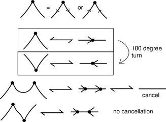
Figure 3: Arrow Convention.

H. A. Dye and L. H. Kauffman studied an equivalent version of the arrow polynomial [DK09] and used it to obtain a lower bound on the virtual crossing number for diagrams of a virtual link. In the Dye-Kauffman version the cusps are replaced by an extra orientation convention. See Figure 3. Here we shall refer to $\langle K\rangle_{A}$ as the arrow polynomial of $K.$ We call the reduced cusp count $n(c)$ for a state loop the arrow number of this loop. Thus a state loop with label $K_{n}$ has arrow number $n.$

Both the extended bracket polynomial and the arrow polynomial $\langle K\rangle_{A}$ are invariant with respect to the second and the third Reidemeister moves. They can be made invariant under the first Reidemeister move by the usual normalisation by a power of $(-A^{3}).$ In the rest of the paper, we shall omit this normalisation. Moreover, while passing to the Khovanov homology, we shall omit the corresponding renormalisation and refer the interested reader to [BN02, Man05b] or [BN02, BN05].

The aim of the present paper is to present two categorifications of the arrow polynomial [Kau09, DK09]. We split the chain spaces of the Khovanov complex ${\cal C}(K)$ into subspaces ${\cal C}_{gr=x}(K)$ with a fixed new grading $x$ and restrict our differential $\partial$ to these subspaces. Now, set $\partial=\partial^{\prime}+\partial^{\prime\prime}$ where $\partial^{\prime}$ is the part of $\partial$ which preserves the new gradings for basic chains, and $\partial^{\prime\prime}$ is the remaining part of $\partial$. We have to define this new grading in such a way that the new differential $\partial^{\prime}$ is well defined and the corresponding homology groups $H({\cal C}(K),\partial^{\prime})$ are invariant with respect to Reidemeister moves.

A Khovanov homology theory for virtual knots has been constructed in a sequence of papers by Manturov. In [Man08], one gives a certain procedure for further generalization of these invariants, which deals with so-called dotted gradings. In working with Khovanov homology we use enhanced states of the Kauffman bracket polynomial. These enhanced states are collections of labelled simple closed curves obtained by smoothing crossings in the diagram. Each curve is labelled with either the algebra element $X$ or with the number $1$. The elements $X$ and $1$ belong to the algebra $k[X]/(X^{2})$ where $k=Z[A,A^{-1}].$ In the dotted grading, the $X$ and the $1$ can acquire a dot in the form $\dot{X}$ and $\dot{1}.$ We explain how this notation works in the discussion below.

We assume all circles in Kauffman states of a diagram can be assigned a mod ${\bf Z}_{2}$ dotting: every state circle is either dotted or not (the dotting should be read from the topology/combinatorics of the diagram), and the new integral grading of a chain is set to be ${\#}{\dot{X}}-{\#}{\dot{1}}$, i.e. the number of dotted circles with the element $X$ minus the number of dotted circles carrying the element $1$. If this dotting satisfies certain very simple axioms [Man08], then the complex is well defined and its homology is invariant under Reidemeister moves.

Another way to introduce the gradings for a given Khovanov homology theory is to take the coefficients like $[S]$ or $\prod_{c(S)}K_{n(s)}$ to be new (multi)gradings themselves, but for this we use ${\bf Z}_{2}$-coefficients. Possibly, this ${\bf Z}_{2}$-reduction can be avoided if we use twisted coefficients similar to those from [Man07b], but this has not been done so far.

We note that this paper makes use of enhanced states of the bracket polynomial for discussing Khovanov homology. This approach was introduced in [Viro1, Viro2]. The first categorification of link invariants in thickened surfaces, thus also of the Kauffman bracket of virtual links occurs in [APS]. Finally, two recent papers by[Caprau, CMW] can also be viewed as categorifying the arrow polynomial. although that was not the principle aim of these works. A sequel to this paper will discuss these relationships.

1.1 Acknowledgements

The last two authors (L.H.K. and V.O.M.) express their gratitude to the Mathematisches Forschungsinstitut-Oberwolfach, where this paper was finished, for a nice creative scientific atmosphere.

2 The Arrow Polynomial $\langle K\rangle_{A}$

In this section we describe the arrow polynomial invariant [Kau09, DK09]. One way to see the definition of the arrow polynomial is to begin with the extended bracket invariant [Kau09] and simplify it. The extended invariant is a sum of graphs (taken up to virtual equivalence in the plane) weighted by polynomials. In the extended bracket one uses an oriented expansion so that the smoothings consist of oriented smoothings and disoriented smoothings. At a disoriented smoothing one sees two cusps with orientation arrows going into the cusp point in one cusp and out of the cusp point for the other cusp. Rules for reducing the states of the extended bracket keep the cusps paired whenever possible. If we release the cusp pairings at the disoriented smoothings, we get simpler graphs. These are composed of disjoint collections of circle graphs that are labelled with the orientation markers and left-right distinctions that occur in the state expansion. The basic conventions for this simplification are shown in Figure 2. In that figure we illustrate how the disoriented smoothing is a local disjoint union of two vertices (the cusps). Each cusp is denoted by an angle with arrows either both entering the cusp or both leaving the cusp. Furthermore, the angle locally divides the plane into two parts: One part is the span of an acute angle (of size less than $\pi$); the other part is the span of an obtuse angle. We refer to the span of the acute angle as the inside of the cusp. In Figure 2, we have labelled the insides of the cusps with the symbol $\sharp.$

Figure 1 illustrates the basic oriented bracket expansion formula. Figure 2 illustates the reduction rule for the arrow polynomial. While we have indicated (above) the relationship of the arrow polynomial with the extended bracket polynomial, the reduction rule for the arrow polynomial is completely described by Figure 2. We shall denote the arrow polynomial by the notation $\langle K\rangle_{A},$ for a virtual knot or link diagram $K.$ The reduction rule allows the cancellation of two adjacent cusps when they have insides on the same side of the segment that connects them. When the insides of the cusps are on opposite sides of the connecting segment, then no cancellation is allowed. All graphs are taken up to virtual equivalence. Figure 2 illustrates the simplification of two circle graphs. In one case the graph reduces to a circle with no vertices. In the other case there is no further cancellation, but the graph is equivalent to one without a virtual crossing. The state expansion for $\langle K\rangle_{A}$ is exactly as shown in Figure 1, but we use the reduction rule of Figure 2 so that each state is a disjoint union of reduced circle graphs. Since such graphs are planar, each is equivalent to an embedded graph (no virtual crossings) and the reduced forms of such graphs have $2n$ cusps that alternate in type around the circle so that $n$ are pointing inward and $n$ are pointing outward. The circle with no cusps is evaluated as $d=-A^{2}-A^{-2}$ as is usual for these expansions and the circle is removed from the graphical expansion. Let $K_{n}$ denote the circle graph with $2n$ alternating vertex types as shown in Figure 2 for $n=1$ and $n=2.$ By our conventions for the extended bracket polynomial, each circle graph contributes $d=-A^{2}-A^{-2}$ to the state sum and the graphs $K_{n}$ (with $n\geq 1$) remain in the graphical expansion. For the arrow polynomial $\langle K\rangle_{A}$ we can regard each $K_{n}$ as an extra variable in the polynomial. Thus a product of the $K_{n}$’s denotes a state that is a disjoint union of copies of these circle graphs with multiplicities. By evaluating each circle graph as $d=-A^{2}-A^{-2}$ we guarantee that the resulting polynomial will reduce to the original bracket polynomial when each of the new variables $K_{n}$ is set equal to unity. Note that we continue to use the caveat that an isolated circle or circle graph (i.e. a state consisting in a single circle or single circle graph) is assigned a loop value of unity in the state sum. This assures that $\langle K\rangle_{A}$ is normalized so that the unknot receives the value one.

Formally, we have the following state summation for the arrow polynomial

$$\langle K\rangle_{A}=\sum_{S}\langle K|S\rangle d^{||S||-1}P[S]$$

where $S$ runs over the oriented bracket states of the diagram, $\langle K|S\rangle$ is the usual product of vertex weights as in the standard bracket polynomial, $||S||$ is the number of circle graphs in the state $S$, and $P[S]$ is a product of the variables $K_{n}$ associated with the non-trivial circle graphs in the state $S.$ Note that each circle graph (trivial or not) contributes to the power of $d$ in the state summation, but only non-trivial circle graphs contribute to $P[S].$ The regular isotopy invariance of $\langle K\rangle_{A}$ follows from an analysis of the behaviour of this state summation under the Reidemeister moves.

Theorem 1.

With the above conventions, the arrow polynomial $\langle K\rangle_{A}$ is a polynomial in $A,A^{-1}$ and the graphical variables $K_{n}$ (of which finitely many will appear for any given virtual knot or link). $\langle K\rangle_{A}$ is a regular isotopy invariant of virtual knots and links. The normalized version

$$W[K]=(-A^{3})^{-wr(K)}\langle K\rangle_{A}$$

is an invariant of virtual isotopy. Here $wr(K)$ denotes the writhe of the diagram $K$; this is the sum of the signs of all the classical crossings in the diagram. If we set $A=1$ and $d=-A^{2}-A^{-2}=-2$, then the resulting specialization

$$F[K]=\langle K\rangle_{A}(A=1)$$

is an invariant of flat virtual knots and links.

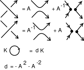
Figure 1: Oriented Bracket Expansion.

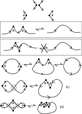
Figure 2: Reduction Relation for the Arrow Polynomial.

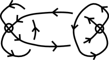
Figure 4: Kishino Diagram.

Example. Figure 4 illustrates the Kishino diagram. With $d=-A^{2}-A^{-2}$

$$\langle K\rangle_{A}=1+A^{4}+A^{-4}-d^{2}K_{1}^{2}+2K_{2}.$$

Thus the simple extended bracket shows that the Kishino is non-trivial and non-classical. In fact, note that

$$F[K]=3+2K_{2}-4K_{1}^{2}.$$

Thus the invariant $F[K]$ of flat virtual diagrams proves that the flat Kishino diagram is non-trivial. This example shows the power of the arrow polynomial. See [Kau09, DK09] for the details of this calculation.

3 Khovanov homology for virtual knots

In this section, we describe Khovanov homology for virtual knots along the lines of [Kho97, BN02, Man07b].

The bracket polynomial [Kau87] is usually described by the expansion

$$\langle\raisebox{-0.25pt}{\includegraphics[width=14.22636pt]{skcrossr.eps}}\rangle=A\langle\raisebox{-0.25pt}{\includegraphics[width=14.22636pt]{skcrh.eps}}\rangle+A^{-1}\langle\raisebox{-0.25pt}{\includegraphics[width=14.22636pt]{skcrv.eps}}\rangle$$ (2)

Letting $c(K)$ denote the number of crossings in the diagram $K,$ if we replace $\langle K\rangle$ by $A^{-c(K)}\langle K\rangle,$ and then replace $A^{2}$ by $-q^{-1},$ the bracket will be rewritten in the following form:

$$\langle\raisebox{-0.25pt}{\includegraphics[width=14.22636pt]{skcrossr.eps}}\rangle=\langle\raisebox{-0.25pt}{\includegraphics[width=14.22636pt]{skcrh.eps}}\rangle-q\langle\raisebox{-0.25pt}{\includegraphics[width=14.22636pt]{skcrv.eps}}\rangle$$ (3)

with $\langle\bigcirc\rangle=(q+q^{-1})$. In this form of the bracket state sum, the grading of the Khovanov homology (which is described below) appears naturally. We shall continue to refer to the smoothings labelled $q$ (or $A^{-1}$ in the original bracket formulation) as $B$-smoothings. We should further note that we use the well-known convention of enhanced states where an enhanced state has a label of $1$ or $X$ on each of its component loops. We then regard the value of the loop $(q+q^{-1})$ as the sum of the value of two circles: a circle labelled with a $1$ (the value is $q$) and a circle labelled with an $X$ (the value is $q^{-1}).$

To see how the Khovanov grading arises, consider the form of the expansion of this version of the bracket polynomial in enhanced states. We have the formula as a sum over enhanced states $s:$

$$\langle K\rangle=\sum_{s}(-1)^{n_{B}(s)}q^{j(s)}$$

where $n_{B}(s)$ is the number of $B$-type smoothings in $s$, $\lambda(s)$ is the number of loops in $s$ labelled $1$ minus the number of loops labelled $X,$ and $j(s)=n_{B}(s)+\lambda(s)$. This can be rewritten in the following form:

$$\langle K\rangle=\sum_{i,\,j}(-1)^{i}q^{j}\left[\sum_{s:{n_{B}(s)=i,\,j(s)=j}}1\right]=\sum_{i\,,j}(-1)^{i}q^{j}dim({\cal C}^{ij}).$$

In the Khovanov homology, the states with $n_{B}(s)=i$ and $j(s)=j$ form the basis for a module ${\cal C}^{ij}$ over the ground ring $k.$ Thus we can write

$$dim({\cal C}^{ij})=\sum_{s:{n_{B}(s)=i,\,j(s)=j}}1.$$

The bigraded complex composed of the ${\cal C}^{ij}$ has a differential $d:{\cal C}^{ij}\longrightarrow{\cal C}^{i+1\,j}.$ That is, the differential increases the homological grading $i$ by $1$ and preserves the quantum grading $j.$ Below, we will remind the reader of the formula for the differential in the Khovanov complex. Note however that the existence of a bigraded complex of this type allows us to further write:

$$\langle K\rangle=\sum_{j}q^{j}\sum_{i}(-1)^{i}dim({\cal C}^{ij})=\sum_{j}q^{j}\chi({\cal C}^{\bullet\,j}),$$

where $\chi({\cal C}^{\bullet\,j})$ is the Euler characteristic of the subcomplex ${\cal C}^{\bullet\,j}$ for a fixed value of $j.$ Since $j$ is preserved by the differential, these subcomplexes have their own Euler characteristics and homology. We can write

$$\langle K\rangle=\sum_{j}q^{j}\chi(H({\cal C}^{\bullet\,j})),$$

where $H({\cal C}^{\bullet\,j})$ denotes the homology of this complex. Thus our last formula expresses the bracket polynomial as a graded Euler characteristic of a homology theory associated with the enhanced states of the bracket state summation. This is the categorification of the bracket polynomial. Khovanov proves that this homology theory is an invariant of knots and links, creating a new and stronger invariant than the original Jones polynomial.

We explain the differential in this complex for mod-$2$ coefficients and leave it to the reader to see the references for the rest. The differential is defined via the algebra ${\cal A}=k[X]/(x^{2})$ so that $X^{2}=0$ with coproduct $\Delta:{\cal A}\longrightarrow{\cal A}\otimes{\cal A}$ defined by $\Delta(X)=X\otimes X$ and $\Delta(1)=1\otimes X+X\otimes 1.$ Partial differentials (which are defined on an enhanced state with a chosen site, whereas the differential is a sum of these mappings) are defined on each enhanced state $s$ and a site $\kappa$ of type $A$ in that state. We consider states obtained from the given state by smoothing the given site $\kappa$. The result of smoothing $\kappa$ is to produce a new state $s^{\prime}$ with one more site of type $B$ than $s.$ Forming $s^{\prime}$ from $s$ we either amalgamate two loops to a single loop at $\kappa$, or we divide a loop at $\kappa$ into two distinct loops. In the case of amalgamation, the new state $s$ acquires the label on the amalgamated circle that is the product of the labels on the two circles that are its ancestors in $s$. That is, $m(1\otimes X)=X$ and $m(X\otimes X)=0$. Thus this case of the partial differential is described by the multiplication in the algebra. If one circle becomes two circles, then we apply the coproduct. Thus if the circle is labelled $X$, then the resultant two circles are each labelled $X$ corresponding to $\Delta(X)=X\otimes X$. If the orginal circle is labelled $1$ then we take the partial boundary to be a sum of two enhanced states with labels $1$ and $X$ in one case, and labels $X$ and $1$ in the other case on the respective circles. This corresponds to $\Delta(1)=1\otimes X+X\otimes 1.$ Modulo two, the differential of an enhanced state is the sum, over all sites of type $A$ in the state, of the partial differential at these sites. It is not hard to verify directly that the square of the differential mapping is zero and that it behaves as advertised, keeping $j(s)$ constant. There is more to say about the nature of this construction with respect to Frobenius algebras and tangle cobordisms. See [Kho97, BN02, BN05]

Here we consider bigraded complexes ${\cal C}^{ij}$ with height (homological grading) $i$ and quantum grading $j.$ In the unnormalized Khovanov complex $[[K]]$ the index $i$ is the number of $B$-smoothings of the bracket, and for every enhanced state, the index $j$ is equal to the number of components labelled $1$ minus the number of components labelled $X$ plus the number of $B$-smoothings. The normalized complex differs from $[[K]]$ by an overall shift of both gradings; the differential preserves the quantum grading and increases the height by $1$. The height and grading shift operations are defined as $({\cal C}[k]\{l\})^{ij}={\cal C}[i-k]\{j-l\}$.

This form is used as the starting point for the Khovanov homology. We now describe the formalism in a bit more detail in order to give the structure of the differential for Khovanov homology of virtual knots and links. For a diagram $K$ of a virtual knot, we consider the state cube defined as follows: Enumerate all $n$ classical crossings of $K$ in arbitrary way and consider all Kauffman states (states as collections of loops without specific enhancement labels) as vertices of the discrete cube $\{0,1\}^{n}.$ Each coordinate corresponds to a way of smoothing and is equal to $0$ (the $A$-smoothing) or $1$ (the $B$-smoothing). Thus, each vertex of the cube defines a set of circles (say, $p$ circles), and this set of circles defines a certain vector space (module) of dimension $2^{p}.$ The module for a single circle is generated by $1$ and $X.$ The spaces together form the total chain space of the unnormalized Khovanov complex $[[K]]$ and its normalized version ${\cal C}[[K]]$. We omit the normalisation, which is standard, and refer the reader to [Kho97, BN02, Man07b].

We regard the loop factors for the unenhanced bracket, $(q+q^{-1}),$ as graded dimensions of the module $V=Span(\{1,X\}),\mbox{deg}\;1=1,\mbox{deg}\;X=-1$ over some ring $k$, and the height $i(s)$ plays the role of homological dimension. Define the chain space $[[K]]_{i}$ of homological dimension $i$ to be the direct sum over all vertices of height $i$ (defined as above) of $V^{\gamma(s)}\{i\}$ (here $\{\cdot\}$ is the quantum grading shift and $\gamma(s)$ is the number of loops in the state $s$). Then the alternating sum of graded dimensions of $[[K]]_{i}$, is precisely equal to the (modified) Kauffman bracket, as we have described above.

Thus, if one defines a differential on $[[K]]$ that preserves the grading and increases the homological dimension by $1$, the Euler characteristic of that complex will be precisely the bracket.

We now consider a generalization of the Khovanov homology to virtual knots. When we pass from one state of the state cube to a neighboring state (which differs precisely at one coordinate), we get a resmoothing of the set of circles. We refer to that as a bifurcation of the state cube. Such a bifurcation can either merge two circles into one ($2\to 1$-bifurcation) or split one circle into two ($1\to 2$-bifurcation), or (in the case of virtual knots and links) transform one circle into one ($1\to 1$-bifurcation). These bifurcations encode the information about differentials in the complex as follows.

We have defined the state cube consisting of state loops and carrying no information how these loops interact. For Khovanov homology, we deal with the same cube, remembering the information about the loop bifurcation. Later on, we refer to it as a bifurcation cube.

The chain spaces of the complex are well defined. However, the problem of finding a differential $\partial$ in the general case of virtual knots, is not easy. See Figure 7 for a key example that we shall discuss. To define the differential, we have to pay attention to the different isomorphism classes of the chain space identified by using local bases (see below).

The differential acts on the chain space as follows: it takes a chain (regard an enhanced state as an elementary chain) corresponding to a certain vertex of the bifurcation cube to some chains corresponding to all adjacent vertices with greater homological degree. That is, the differential is a sum of partial differentials, each partial differential acts along an edge of the cube. Every partial differential corresponds to some direction and is associated with some classical crossing of the diagram. The total differential is the sum of these partial differentials, and so formally looks like

$$\partial=\sum_{a}\partial_{a}$$

where the summation is over all edges of the cube. In discussing differentials we shall often refer to a partial differential without indicating its subscript.

Selecting an un-enhanced Kauffman state $S$ (consisting of loops with cusps), we choose an arbitrary order for the circles in S. and then orient each circle in $S$. Letting $\gamma(S)=||S||$ be the number of loops in $S$, associate the module $\Lambda^{||S||}(V)$ to $S$ where this denotes the $||S||^{th}$ exterior power of $V$ – the order of the factors in the exterior power depends on the choice of the ordering that was chosen. Having made this choice (of ordering and orientation), if $s$ is an enhancement of $S$ then label all loops in the state $s$ with either $+X$ or $+1$ according to the enhancement. This oriented, ordered, and labelled state forms a generating chain in the complex. If the orientation of a loop in $S$ is reversed then the label for $X$ becomes $-X$ but the label for $1$ does not change. Otherwise, signs change according to the structure of the exterior algebra.

Then for a state with $l$ circles, we get a vector space (module) of dimension $2^{l}$. All these chains have homological dimension $i=n_{B}$. We set the quantum grading $j$ of these chains equal to $i$ plus the number of circles marked by $\pm 1$ minus the number of circles marked by $\pm X$.

Let us now define the partial differentials of our complex. First, we think of each classical crossing so that its edges are oriented upwards, as in Figure 5, upper left picture.

Choose a certain state of a virtual link diagram $L\subset{\cal M}$. Choose a classical crossing $U$ of $L$. We say that in a state $s$ that a state circle $\gamma$ is incident to a classical crossing $U$ if at least one of the two local parts of smoothed crossing $U$ belongs to $\gamma$. Consider all circles $\gamma$ incident to $U$. Fix some orientation of these circles according to the orientation of the edge emanating in the upward-right direction and opposite to the orientation of the edge coming from the bottom left, see Figure 5. Such an orientation is well defined except for the case when resmoothing one edge takes one circle to one circle. In such a situation, we shall not define the local basis $\{1,X\}$, and we set the partial differential corresponding to that edge to be zero.

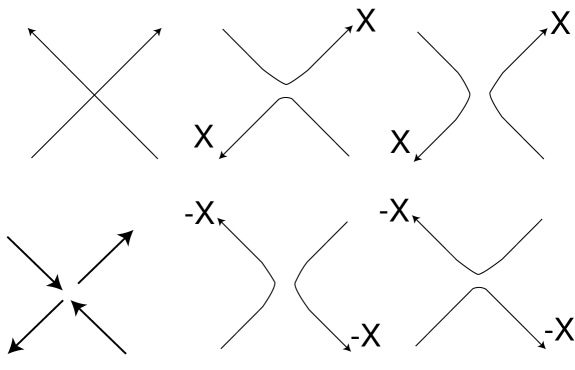
Figure 5: Setting the local basis for a crossing

In the other situations, the edge of the cube corresponding to the partial differential either increases or decreases the number of circles. This means that at the corresponding crossing the local bifurcation either takes two circles into one or takes one circle into two. If we deal with two circles incident to a crossing from opposite signs, we order them in such a way that the upper (resp., left) one is the first one; the lower (resp., right) one is the second; here the notions “left, right, upper, lower” are chosen according to the rule for identifying the crossing neighbourhood with Figure 5. Furthermore, for defining the partial differentials of types $m$ and $\Delta$ (which correspond to decreasing/increasing the number of circles by one) we assume that the circles we deal with are in the initial positions specified in our ordered tensor product; this can always be achieved by a preliminary permutation, which, possibly leads to a sign change. Now, let us define the partial differential locally according to the prescribed choice of generators at crossings and the prescribed ordering.

Now, we describe the partial differentials $\partial$ from [Man07b] without new gradings. If we set $\Delta(1)=1_{1}\wedge X_{2}+X_{1}\wedge 1_{2};\Delta(X)=X_{1}\wedge X_{2}$ and $m(1_{1}\wedge 1_{2})=1;m(X_{1}\wedge 1_{2})=m(1_{1}\wedge X_{2})=X;m(X_{1}\wedge X_{2})=0$, define the partial differential $\partial$ according to the rule $\partial(\alpha\wedge\beta)=m(\alpha)\wedge\beta$ (in the case we deal with a $2\to 1$-bifurcation, where $\alpha$ denotes the first two circles $\alpha$) or $\partial(\alpha\wedge\beta)=\Delta(\alpha)\wedge\beta$ (when one circle marked by $\alpha$ bifurcates to two ones); here by $\beta$ we mean an ordered set of oriented circles, not incident to the given crossings; the marks on these circles $\pm 1$ and $\pm X$ are given.

Theorem 2.

[Man07b] Let $K$ be a virtual knot or link. Then $[[K]]$ is a well-defined complex with respect to $\partial.$ After a small grading shift and a height shift, the homology of $[[K]]$ is invariant under the generalised Reidemeister moves for virtual knots and links.

4 Grading Considerations for the Arrow Polynomial $\langle K\rangle_{A}$

In order to consider gradings for Khovanov homology in relation to the structure of the arrow polynomial $\langle K\rangle_{A}$ we have to examine how the arrow number of state loops change under a replacement of an $A$-smoothing by a $B$-smoothing. Such replacement, when we use oriented diagrams involves the replacement of a cusp pair by an oriented smoothing or vice versa. Furthermore, we may be combining or splitting two loops. Refer to Figure 6 for a depiction of the different cases. This figure shows the three basic cases.

In the first case we have two loops $C_{1}$ and $C_{2}$ sharing a disoriented site and the smoothing is a single loop $C$ where the paired cusps of the disoriented site disappear. In this case if $n(C_{1})=n$ and $n(C_{2})=m$, then $n(C)=|n-m|.$

In the second case, we have a single loop $C$ with a disoriented site and a pair of cusps, and on smoothing this site we obtain two loops $C_{1}$ and $C_{2}$ whose arrow numbers are $n(C_{1})=n$ and $n(C_{2})=m.$ The following arrow numbers for $C$ are then possible $|n(C)|=|n-m|$ or $|n+m|.$

In the third case, we have a single loop $C$ with a disoriented site and a pair of cusps, and on smoothing this site we obtain a single loop $C^{\prime}$. Assuming that $n(C^{\prime})=|n+m|$ as shown in the figure, we have $|n(C)|=|n+m+1|$ where $n$ and $m$ can be positive or negative.

These are all the ways that loops can interact and change their respective arrow numbers. In the next section, we will apply these results to the grading in Khovanov homology.

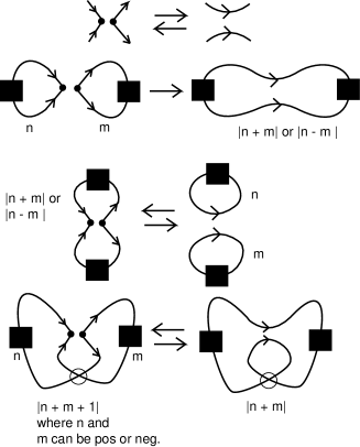
Figure 6: Arrow Numbers for Interacting Loops

5 Dotted gradings and the dotted categorification

First, we introduce a concept of dotting axiomatics as developed in [Man08]. The purpose of this dotting axiomatics is to give general conditions under which extra decorations on the states can be used to create new gradings and hence new versions of Khovanov homology. We will apply these axiomatics to the arrow numbers on the state loops of the arrow polynomial.

For the axiomatics, assume we have some class of objects with Reidemeister moves, Kauffman bracket and the Khovanov homology (in the usual setup or in the setup of [Man05c]). Assume that there is a method, which for every diagram and every state of it associates dots to some of the circles in the bracket states in such a way that the following conditions hold:

1. The dotting of circles is additive with respect to $2\to 1$-bifurcations and $1\to 2$-bifurcations mod $2$. This additivity means that when we merge two circles (split one circle into two), the number of dots on the circles being operated on is preserved modulo ${\bf Z}_{2}$.

   This means that the parity of the number of dots on the circles operated on is preserved whenever we merge two circles or split one circle into two.

   If the dotting is not preserved under a $1\to 1$ bifurcation, then this bifurcation is taken to be the zero map.

2. Similar curves for corresponding smoothings of the RHS and the LHS of any Reidemeister move have the same dotting.

3. Small circles appearing for the first, the second, and the third Reidemeister moves are not dotted.

Let us call the conditions above the dotting conditions. With such a structure in hand, one defines a new grading $g(s)$ for states $s$ by taking the difference between the number of dotted $X$’s and the number of dotted $1$’s in the state.

$$g(s)=\sharp({\dot{X}})-\sharp({\dot{1}})$$

We shall use this grading in the constructions that follow.

Theorem 3.

Assume there is a theory using the Khovanov complex $([[K]],\partial)$ such that the Kauffman states can be dotted so that the dotting conditions hold. Take $[[K]]_{g}$ to be the space $[[K]]$ endowed with new grading as above.

Define $\partial^{\prime}$ to be the composition of $\partial$ with the new grading projection and set $\partial^{\prime\prime}=\partial-\partial^{\prime}$.

Then the homology of $[[K]]_{g}$ (with respect to $\partial^{\prime}$) is invariant (up to a degree shift and a height shift).

For any operator $\lambda$ on the ground ring, the complex $[[K]]_{g}$ is well defined with respect to the differential $\partial^{\prime}+\lambda\partial^{\prime\prime}$, and the corresponding homology is invariant (up to well-known shifts).

Moreover, if we have several forms of dotting $g_{1},g_{2},\dots,g_{k}$ occuring together on the same Khovanov complex so that for each of them the dotting condition holds, then the complex $K_{g_{1},\dots,g_{k}}$ with differential $\partial_{g_{1},\dots,g_{k}}$ defined to be the projection of $\partial$ to the subspace preserving all the gradings, is invariant.

The theorem above allows one to ‘raise’ some additional information modulo ${\bf Z}_{2}$ to the level of gradings. Our aim is to categorify the arrow polynomial, that is, to add new gradings corresponding to the arrow count: for every state we have a set of circles labelled by a set of non-zero integers, and this set of integers should be represented in the complex as a grading. Theorem 3 shows that it is possible to do that when we consider the information of the arrow count only modulo ${\bf Z}_{2}$: the conditions of additivity and similarity under Reidemeister moves for arrow count were checked in the previous section of this paper.

In order to use the integral information about the arrow count, we have to undertake a generalization of the construction of theorem 3. We shall do this in the next section. This section of the paper is devoted to describing a first-order categorification of the arrow polynomial.

The main idea behind the proof of Theorem 3 is as follows. Additivity of the grading can be verified and checked on a bifurcation cube. First of all, it follows from a straightforward check that $\partial^{\prime\prime}$ always increases the dotted grading (this is proved in [Man07b] but can be taken here as an exercise for the reader). Then, the complex is well defined because $(\partial^{\prime})^{2}$ is nothing but a composition of $(\partial)^{2}$ with a “grading-preserving projection”. This is guaranteed because $\partial^{\prime\prime}$ strictly increases the new grading. Note the the mod-2 preservation of the dotting is what makes this grading increase of $\partial^{\prime\prime}$ work. thus Theorem 3 depends ultimately on that parity presevation of the dotted grading.

The main idea of the invariance under Reidemeister moves is similar to the usual Khovanov idea, see for example [BN02]: we have to check that the multiplication $m$ remains surjective after reducing $\partial$ to $\partial^{\prime}$ and $\Delta$ remains injective. The latter follows from the fact that “small circles are not dotted”.

Now, one can easily check that the conditions of the theorem hold if we set the dotting as follows: the curve is dotted if it is marked as $K_{j}$ with $j$ odd, and it is not dotted if it is marked as $K_{i}$ with $i$ even.

Now, one checks that

1. The dotting is ${\bf Z}_{2}$-additive with respect to resmoothing (performing $1\to 2$ or $2\to 1$ bifurcation).

   This follows from Figure 6 upper part: we see that when merging two circles with arrow count $m$ and $n$, we get $\pm m\pm n$ and when splitting a circle with arrow number $k$, we get two circles with arrow numbers $l$ and $\pm k\pm l$ which results in ${\bf Z}_{2}$-additivity under $2\to 1$ and $1\to 2$-bifurcations.

   On the other hand, if partial differentials for all $1\to 1$ bifurcations are set to be zero, it can be checked that all faces having at least $1\to 1$-bifurcation are anticommutative because $0=0$. The only non-trivial example is shown in Figure 7, and the corresponding calculation is performed in [Man07b].

2. The small circles coming from Reidemeister moves are not dotted. Indeed, for the 1st Reidemeister move we have no cusps at all, and for the second move and for the third move we have two cusps of opposite signs.

3. For any Reidemeister move, the corresponding state diagrams in the LHS and RHS have the same dotting. Locally, there is no grading change for the Reidemeister moves when we use arrow counts. Again, this follows from the invariance under Reidemeister moves: two pictures would not get cancelled if they had different coefficients coming from cusps; this means they have the same dotting.

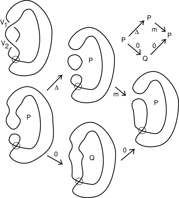
Figure 7: A face for the case of the extended bracket of the cube

6 ${\bf Z}_{2}$-categorification with general gradings

6.1 General setup

The aim of this section is to prove a general theorem on categorification that fits the arrow polynomial. This is an extension of the dotted grading construction, which works, however, only with ${\bf Z}_{2}$-coefficients for the homology. Later, we shall discuss whether this construction can be extended to the case of integral coefficients. For instance, we can extend this construction to the case of integral coefficients if the odd Khovanov homology theory [ORS07] can be defined for this class of knots.

Briefly, we want to start with a Khovanov homology (usual over ${\bf Z}_{2}$ or the one using twisted coefficients) and make some partial differentials equal to zero.

As the initial data for this theorem, we require that we have a well-defined bracket, and we assume that in each state of the diagram, each circle is given a non-negative integer. For the dotted conditions, we require that

1. The numbers are “plus-minus additive” with respect to $2\to 1$-bifurcations and $1\to 2$-bifurcations, that is, if a resmoothing of two circles labelled by non-negative integers $p$ and $q$ leads to one circle, the label of this circle will be $|p+q|$ or $|p-q|$.

2. Similar curves for corresponding smoothings of the RHS and the LHS of any Reidemeister move have the same numbers.

3. Small circles appearing for the first, the second, and the third Reidemeister moves are labelled by zeroes.

We call these conditions integer labelling conditions.

After this, our strategy will be as follows: If we attempt to make the integral arrow count the new grading and take the part of the differential preserving this, to be the new differential, we shall see that the square of this new differential will not be zero. Consider the situation when a $2$-face of the bifurcation cube has arrow counts $P$ in the left corner (both smoothings zero), $P$ in the upper corner (both smoothings one), $P$ in one right corner and $Q$ in the remaining corner. See Figure 7 for an example. Then one composition of the two differentials (going through $P$) survives, while the other one (going through $Q$) becomes zero. That is why the square of the new proposed differential, detecting the arrow count, is non-zero. On the other hand, all the information about the arrow count has to be included in order to get a faithful categorification of the arrow polynomial (that is, having a chain space with gradings one can restore the arrow count, and having the homology one can restore the arrow polynomial). In order to solve this problem, we are going to introduce two new sorts of gradings, one of which will correct the other, and make the differential well-defined.

We take the usual Khovanov differential $\partial$ and form two new series of gradings (called multiple gradings and vector gradings). After that, for each basic chain of the complex we have a whole collection of gradings, and we define the new differential $\partial^{\prime}$ to be the composition of $\partial$ with the projection to the subspace where all gradings are preserved by $\partial$, having the same gradings (all multiple and vector gradings) as in the preimage. That is, we let $S=\{x|gr(x)=gr(\partial x)\}$ and define $\partial^{\prime}=\partial|_{S}.$

Now, we introduce multiple gradings as follows. A multiple grading is a set of strictly positive integers that is associated with a Kauffman state of the diagram. That is,the state is not yet labelled with $X$ and $1$; a basic chain in the state is such a labelling. With each state, we shall associate exactly one multiple grading for each basic chain in this state, independently from the particular choice of $X$ and $1$ on circles. This multiple grading is just the set of all non-zero arrow counts on circles of the state.

The vector grading is an infinite ordered collection (list) of integers (first, second, third, etc.) each of which might be either positive or negative or zero. The vector grading depends on the particular choice of $1$ and $X$ on all state circles. But before introducing the vector grading, we introduce the vector dotting for state circles (that have the initial labelling by arrow numbers). For a circle labelled by $p$ we put no dots at all if $p=0$; otherwise we represent $p=2^{k-1}{l}$, where $l$ is odd and put exactly one dot of order $k$ over this circle (we also call it a $k$-th dot). Thus, for $p=1$ we will have only one primary dot, for $p=2$ we will have only one secondary dot, for $p=4$ we will have only one ternary dot and so on. The vector dotting is an infinite vector of these dot numbers with one possibly non-zero coordinate for each state circle. Note that the vector dotting depends only on arrow numbers for the Kauffman state.

Now we can define the vector grading. The vector grading of a trivial circle (without dots) is the zero vector $(0,\dots,0,\dots)$. For a non-trivial circle having one $k$-th dot, the grading is set to be $+1$ on $k$-th vector position for the enhanced state carrying $X$ and $-1$ on $k$-th vector position for the enhanced state carrying $1$; the other entries of the vector grading for a given enhanced state circle are set to be zero.

The vector grading of a basic chain (enhanced state) is defined to be the coordinatewise sum of the vector gradings (these are infinite vectors) over all circles in the enhanced state. Thus, if we have one circle labelled by $2$ with element $X$ on it and another circle labelled by $1$ with element $1$ on it, we get the vector grading: $(-1,1,0,\dots,0,\dots)$.

The chain space of the initial Khovanov complex is split into subspaces with respect to the multiple grading and vector grading. We set the differential $\partial^{\prime}$ to be the composition of the initial differential $\partial$ with the projection to the subspace having the same gradings as the preimage.

Theorem 4.

If a state labelling satisfies the integer labelling conditions, then the complex ${\cal C}$ is well defined with respect to differential $\partial^{\prime}$ (that is, $(\partial^{\prime})^{2}=0$), and its homology groups $H({\cal C},{\partial^{\prime}})$ are invariant with respect to the Reidemeister moves.

First, let us check that the arrow polynomial statisfies the integer labelling conditions. This follows from Figure 6. Now, the second condition “similar curves generate similar smoothing” also follows from a direct calculation, as well as the third condition about trivial circles coming from Reidemeister moves. Indeed, for the first Reidemeister move one gets a small loop without any cusp, for the second Reidemeister move one gets either a loop without cusps or a loop with two cusps cancelling each other. The same for the third Reidemeister move: one gets at least two cusps, which should cancel each other. This proves that the integer labelling conditions hold for the arrow count.

Now, let us prove the main theorem. The proof will consist of the two parts: the difficult one, where we show that the complex is well defined (the square of the differential is zero) and the easy one, where we prove that the homology is invariant under Reidemeister moves. The second part will be standard and in main features it will repeat the analogous proof for the usual Khovanov homology.

Part 1. Proof that the complex is well defined.

We first note that we work over ${\bf Z}_{2}$-coefficients. We have to prove that for every $2$-face of the bifurcation cube, the two compositions corresponding to faces will coincide. This means that commutativity and anticommutativity coincide.

An atom is a pair $(M,\Gamma)$ of a $2$-manifold $M$ and a graph $\Gamma$ embedded $M$ together with a colouring of $M\backslash\Gamma$ in a checkerboard manner. Here $\Gamma$ is called the frame of the atom, whence by genus (resp., Euler characteristic) of the atom we mean that of the surface $M$.

With a virtual knot diagram (with every component having at least one classical crossing) we associate an atom as follows. (Note that the atom need not be orientable). We take all classical crossings to be vertices of the frame. The edges of the frame correspond to branches of the diagram connecting classical crossings (we do not take into account how they intersect in virtual crossings). Moreover, the edges of the frame emanating from a vertex are naturally split into two pairs of opposite ones: the opposite relation (ordering of edges) is taken from the plane diagram. Thus we get two pairs of opposite edges (opposite in the sense that these edges are not adjacent in the cyclic order of edges about the vertex) and also four angles generated by pairs of adjacent (non-opposite) edges. Now, for the obtained four-valent graph we attach black and white cells as follows: for every crossing we indicate two pairs of adjacent edges for “pasting the black cells”, and the remaining pair of angles are used for attaching black cells. Cells are attached globally to conform these local conditions. The “black angles” correspond to pairs of edges taken from the $B$-smoothing of the bracket. This completely defines the way for attaching black and white cells to get a $2$-manifold starting from the frame.

This atomic terminology is useful in classifying virtual diagrams in terms of orientability and non-orientability of the corresponding atoms. An atom has a $1\to 1$-bifurcation if and only if it is non-orientable [Man07b]. In the following we shall need to discuss all atoms that derive from diagrams with two crossings. The reader can easily enumerate the possible Gauss codes with two symbols and arrive at the possibilities $(11)(22)$ (two components, four cases depending on the crossings), $(12)(12)$ (a Hopf link configuration with four crossing possibilities), $(1122)$ (a single unknotted component), $(1212)$ (a non-orientable atom). These cases need to be analyzed and the reader will find them depicted in Figures 8. See also Figures 9 through 12.

Each possible $2$-face of the bifurcation cube represents an atom with $2$ vertices (that is, the face represents all four possibilities for smoothing a pair of crossings in the original link diagram): for each atom, there are four states $AA,AB,BA,BB$ and four maps corresponding to partial differentials $AA\to AB,AA\to BA,AB\to BB,BA\to BB$. Some of them correspond to $1\to 1$-bifurcation which means that the corresponding partial differential in the usual Khovanov complex is zero. Thus, so is the partial differential in question (it is a composition of zero map with a projection). By parity reasons, for a given atom, there may be $4,2$ or $0$ partial differentials (in the initial cube) which are equal to zero.

If all four differentials are equal to zero, then we get the desired equality for the composition of the differentials as $0=0$. If we have $2$ maps of type $1\to 1$ then two options are possible. In one of them we have one zero map for each of the two compositions, which leads to $0=0$. We call such atoms inessential. In the other case we have $0$ for the composition of the two $1\to 1$ maps, but the other composition of maps must be analyzed.

Thus we are left with $6$ essential atoms as shown in Figure 8.

For each of these atoms the usual Khovanov differential produces a commutative diagram. Now, multi-gradings and multi-dotted gradings come into play. We have to show that for each atom $V$ the equality of partial differentials $q\circ p=s\circ r$ for the usual Khovanov differentials will hold for the reduced differentials $q^{\prime}\circ p^{\prime}=s^{\prime}\circ r^{\prime}$. Here $p,q,r,s$ denote the four partial differentials that occur in the Khovanov complex at the atom in question. Some remarks are in order.

Notation. Let us denote the differential of the Khovanov complex by $\partial$, and denote its combination with the projection respecting the multiple grading by $\partial_{multi}$, its combination with the projection respecting the vector gradings by $\partial_{vect}$ and denote the combination with both projections by $\partial^{\prime}$. We are mostly interested in the cases when $\partial=\partial^{\prime}$ or when $\partial^{\prime}=0$ for some particular element of the chain complex.

We have to list all atoms with two vertices. Some of them are disconnected in the sense that there is no edge connecting one vertex to the other.

For such atoms the (anti)commutativity obviously holds.

Now, let us list all connected essential atoms. There are exactly $6$ of them, one non-orientable, $3$ orientable with the frame of the unlink and $2$ orientable with the frame of the Hopf link, see Figure 8.

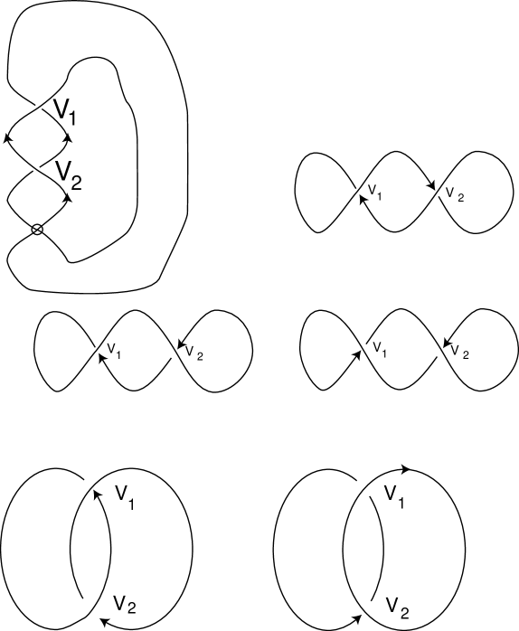
Figure 8: Essential atoms with 2 vertices

For each atom, the anticommutativity of the virtual Khovanov homology over ${\bf Z}$ is checked in [Man07b], which leads to the (anti)commutativity over ${\bf Z}_{2}$. Our goal is to check that the multigradings and dotted multigradings preserve this (anti)commutativity.

For this sake we must consider all possible labellings of the state circles for atoms. Each labelling gives a number of integers, for which we take only absolute values and consider only non-zero ones. This leads to the following multiple gradings $P,Q,R,S$ where $P$ corresponds to the smoothing of the atom where both crossings have $A$-type of smoothing, for $S$ both crossings have $B$-type of smoothing, and for each of $Q,R$ one crossing has $A$-smoothing and the other one has the $B$-smoothing. See Figure 9.

We must look at the differentials depending on $P,Q,R,S$. Denote the corresponding partial differentials of $\partial^{\prime}$ by $f_{1},f_{2},f_{3},f_{4}$, respectively, see Figure 9.

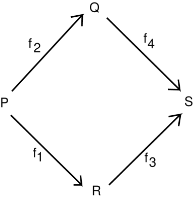
Figure 9: Each atom generates a labelling and two compositions of maps

The following lemma holds.

Lemma 1.

If the multiple gradings $P,Q,R,S$ as described above are all equal ($P=Q=R=S$), then for all partial differentials corresponding to the atom under discussion, we have $\partial_{mult}=\partial$.

Let us now look at vector gradings. There is one case when $\partial_{vect}\neq\partial$ because of the following. Assume we have a $1\to 2$ or $2\to 1$-bifurcation where all three circles are dotted: two circles have dotting of order $k$ and one circle has dotting of higher order $l>k$. This may happen, e.g., in $2\to 1$-bifurcation, when the two circles to merge have arrow label one each (one primary dot) and one target circle has arrow label $2$. In this case $\partial_{vect}\neq\partial$ because the non-trivial secondary dot leads to either $+1$ or $-1$ in the vector grading, hence a non-trivial higher order grading.

Note that this situation does not depend on the particular choice of chain ($1$ or $X$ in a given state). It depends only on the labelling in the two neighboring states. We call this shifting in the vector grading the odd dotting condition.

The following Lemma follows from the definition of the vector grading.

Lemma 2.

If for an atom we have $P=Q=R=S$ then the odd dotting condition does not hold for any of the four edges of the bifurcation diagram.

Now, it turns out that $\partial_{vect}$ in some cases can play the role of the differential, that is, in some cases, $\partial_{vect}^{2}=0$.

Namely, we have the following

Lemma 3.

If the odd dotting condition fails, then $\partial$ does not decrease the vector grading, that is, $\partial=\partial_{vect}+{\tilde{\partial}}$ where $\partial_{vect}$ preserves the vector grading and ${\tilde{\partial}}$ increases exactly one of the dotted gradings (one of the vector slots) by $2$.

Proof.

We deal with a $2\to 1$-bifurcation or $1\to 2$-bifurcation. We may assume that precisely two of the $3$ circles are dotted; moreover, without loss of generality, we may think that these two circles have a primary dot.

Then we have to list all possible maps $m$ and $\Delta$ to see that some of them preserve the vector grading, and the others increase the vector grading by $2.$ Note that all calculations occur in one vector slot since the odd dotting condition fails. In this context we can speak freely about the dotted grading and whether it increases or decreases under a differential.

Let us start with the multiplication. We see that the multiplication of $1$ (without dot) with any of $1$, ${\dot{1}}$, $X$, ${\dot{X}}$ leads to $1$, ${\dot{1}}$, $X$, ${\dot{X}}$ and this multiplication preserves the dotted grading. Now, ${\dot{1}}\otimes{\dot{X}}$ (or ${\dot{X}}\otimes{\dot{1}}$) multiply to get $X$, which does not change the dotted grading. Multiplication of $X$ (or ${\dot{X}}$) with another $X$ (or ${\dot{X}})$ gives zero.

Finally, ${\dot{1}}\otimes{\dot{1}}\to 1$ increases the dotted grading by $2$ as well as any of ${\dot{1}}\otimes X\to{\dot{X}}$ or $\dot{X}\otimes 1\to{\dot{X}}$.

With comultiplication the situation is quite analogous. When none of the three circles is dotted, then the dotted grading is preserved under multiplication. If the circle in the source space and one circle in the target space is dotted, then the comultiplication looks like ${\dot{1}}\to{\dot{1}}\otimes X+{\dot{X}}\otimes 1$ or ${\dot{X}}\to{\dot{X}}\otimes X$. Here the only term where the dotted grading is not preserved, is ${\dot{1}}\to{\dot{X}}\otimes 1$; in this case it is increased by $2$.

If the circle in the source space is not dotted and both circles in the target space are dotted then the dotting is preserved for $1\to 1\otimes X+X\otimes 1$, and it is increased by $2$ for $X\to X\otimes X$. ∎

Altogether Lemmas 2 and 3 lead to the following

Lemma 4.

Assume for an atom representing a face of the bifurcation cube the labellings of all four states coincide. Then the restriction of $(\partial^{\prime})^{2}$ to this atom gives zero.

Proof.

We see that the differentials $\partial$ and $\partial_{mult}$ agree along the edges of such an atom because of Lemma 1, so the $2$-face corresponding to that atom $\partial_{mult}$ (anti)commutes. Moreover, by Lemma 2, the differential $\partial$ splits into the sum of two differentials, $\partial^{\prime}+\partial^{\prime\prime}$, where $\partial^{\prime\prime}$ strictly increases the multi-dotted grading. This means that $(\partial^{\prime})^{2}=0$ because $(\partial^{\prime})^{2}$ is a composition of $(\partial^{2})=0$ with the projection to the “dotted-grading preserving subspace” ∎

The next lemma is obvious.

Lemma 5.

Assume in the setting above $P\neq S$. Then both compositions for our atom are zero maps because of the multi-grading. Thus, the restriction of $(\partial^{\prime})^{2}$ to this atom is zero.

Proof.

This happens just because $\partial^{\prime}$ preserves the multi-grading, and so does $(\partial^{\prime})^{2}$. ∎

In the third case we have $P=Q=S\neq R$ or $P=R=S\neq Q$.

In this case, we must separately consider all the six atoms (the schema representing each atom depicted as in Figure 9) to show that the corresponding faces of the cube anti-commute. We shall draw each atom separately in referring to the appropriate Figures in the paper.

Consider the upper left atom depicted in Figure 8. We leave it to the reader to label the maps so that $f_{2}$ and $f_{4}$ correspond to $1\to 1$-bifurcations. The composition $f_{4}\circ f_{2}$ is then a zero-map, by definition. The remaining two maps are labelled $f_{1}$ and $f_{3}.$

Thus, we have two options. If $R\neq P$ then the other composition of differentials is zero because of multiple gradings. If $P=R=S$ then in the $A$-state we have only one circle labelled by $P$ as well as in the $B$-state; in the intermediate state we have two circles labelled by $P$ and $0$.

The composition $f_{3}\circ f_{1}$ behaves as follows. First, we comultiply $1$, and then we multiply the result. If we start with $X$, we would end up with $0$ because $X\to X\otimes X\to 0$ even for the usual differential $\partial$. If we had $1$ then two options are possible. If $P=0$ then the composition $f_{3}\circ f_{1}$ will lead to $1\to 1\otimes X+X\otimes 1\to X+X=0$. If $P\neq 0$ then the $f_{3}\circ f_{1}$ will take $1$ to $0$ as well because of the vector grading: the vector grading of $1$ for a non-zero $P$ differs from that for $X$ by sign.

Thus, for the unique non-orientable essential atom with two vertices we have the equality $f_{4}\circ f_{2}=0=f_{3}\circ f_{1}$, which shows the (anti)commutativity. For the other atom with the same frame (which corresponds to the Hopf link with the $A$-state having $2$ circles) the “bad” situation does not occur, just because two single-circle states can not have different $K_{j}$’s. This completes the analysis of the upper left atom in Figure 8.

We now consider the remaining five essential atoms in Figure 8. The atoms are all orientable, so the arrow count (labelling) is additive. Following the methodology of our previous argument, we can verify that the anticommutativity survives after the new grading is imposed for these atoms.

The unlink (bottom right in Figure 8) has one circle in the opposite states and two circles in the intermediate states (see the upper part of Figure 10). The Hopf link has 2 circles in the A-state, 2 circles in the B-state, and 1 circle in each of the two intermediate states, as shown in the lower part of Figure 10.

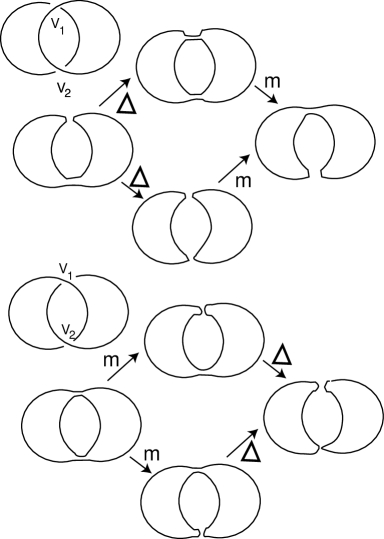
Figure 10: The two atoms with the shadow of the Hopf link

Consider the three atoms having the frame of the unknot with two curls as shown in Figure 8. The corresponding bifurcation cubes have a state with three circles, two states with two circles and one state with one circle (that is positioned opposite the state with three circles). The three possible bifurcation cubes depend on the number of circles in the initial state of the cube. An example of this is shown in Figure 11.

For the Hopf link, assume that for both $2$-circle states the multiple grading is the same as that of one of the two $1$-circle states. By definition, this means that one of the two circles in one $2$-circle state has arrow count zero. Denote the arrow count for the other circle by $p$. Consequently, the other way of merging the two circles gives us $p$ again. This means that the labelling is $A=B=C=D=\{p\}$, and we are in the situation of Lemma 4.

If we have $1$-circle in the $A$-state and $1$-circle in the $B$-state, we may have a “bad” situation $(P=Q=S\neq R)$ (not covered by Lemmas 4 and 5) occurring as described below.

First, note that if $P=Q=S$ then the $A$-state with two circles should have labelling $\{P\}$ as well as the $B$-state, whence the labelling for two circles corresponding to $Q$ should be $\{P,0\}$. We are interested in the case when the other intermediate state has labelling $R=(\alpha,\beta)$, say, $(\alpha,P\pm\alpha)$, where $\alpha\neq 0$.

In this case the composition $f_{3}\circ f_{1}$ is zero. Let us consider the composition $f_{4}\circ f_{2}$.

First, let us consider the partial differentials corresponding to $\partial.$ If we apply it to $X$, we get $0$, because the comultiplication $f_{1}$ gives us $X\otimes X$ and the further multiplication gives zero. On the other hand, the composition $f_{4}\circ f_{2}$ takes $1$ to $0$ because we first get $1\otimes X+X\otimes 1$, which is then mapped to $2X=0$. Now, when we pass from $\partial$ to $\partial^{\prime}$, we see that both multiplication and comultiplication either preserve the vector grading or increase it by $2$, we should compare the dotting of the initial $1$ and the final $X$. If they both are zero, then the composition takes $1$ to $2X=0$, otherwise, $1$ is taken to $0$ because of the dotted gradings.

Note that this is precisely the case where we need our coefficients to be defined over ${\bf Z}_{2}$.

Finally, all 3 atoms with the frame an unknot (drawn in the middle of Figure 8) are to be double-checked.

The three possibilities are: the $A$-state has $3$ circles, or it has $2$ circles or it has $1$ circle, see Figure 11.

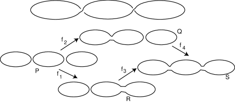
Figure 11: An atom with 2 vertices

Assume $P=Q=S$ (the case $P=R=S$ is analogous because of the symmetry). We claim that in this case $R=P$. Indeed, since we have $3$ circles in the $A$-state, and one circle in the $B$-state, we see that the labellings of the circles are $\{p,0,0\}$ in the $A$-state and $\{p\}$ in the $B$-state. This yields that $R=\{p,0\}=\{p\}$, and the (anti)commutativity follows from Lemma 4.

The atom when we have three circles in the $B$-state is analogous.

In fact, because of the symmetry, we can reduce these three cases to two cases: when we have $1$ and $3$ at the ends, or when we have $2$ and $2$ at the ends.

Now, we are left with the example shown in Figure 12.

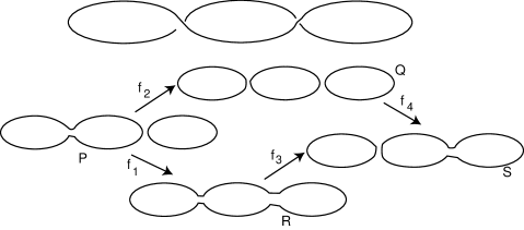
Figure 12: An atom with 2 vertices

We are interested in the case when $P=S$ and either $Q\neq P$ or $R\neq P$.

Note that each of $P$ and $S$ consists of $2$ circles. Assume $P=S=\{a,b\}$.

It is easy to see that if $R=P=S$ then $Q=P=S=R$. Indeed, if $R=S$, this means that both $P$ and $S$ are of the form $\{a,0\}$ (or both are $\{b,0\}$) which yields $Q=\{a,0,0\}=P=S$.

Thus we are interested in the case when $a\neq 0,b\neq 0$ and $Q=P=S$. This means that $Q=\{a,0,b\}$, whence $R$ may be of the form $\{|a\pm b|\}.$ In this case the composition $f_{3}\circ f_{1}=0$ because $Q\neq P$. Let us show that the composition $f_{4}\circ f_{2}=0$.

Recall that both $f_{4}$ and $f_{2}$ are compositions of the partial differential $\partial$ with the projection map preserving the multi-grading and the multi-dotted grading.

Regardless any grading, $f_{4}\circ f_{2}$ would take $1\otimes 1\to 1\otimes X+X\otimes 1$, $1\otimes X\to X\otimes X$, $X\otimes 1\to X\otimes X$.

Now we note that none of these maps survives after applying the projection with respect to vector grading. Indeed, consider for instance the map from $1\otimes 1$ to the summand $1\otimes X$. In the source space we had $1$ and $1$ with vector grading coming from labelling $a$ and $b$; let us denote it by $1_{a}+1_{b}$. For $1\otimes X$ we have either $1_{a}\otimes X_{b}$ or $1_{b}\otimes X_{b}$ depending on the circle having label $a$.

Here $1_{a}$ denotes the $(0,\dots,0,-1,0,\dots,0)$ with the only non-trivial entry on $k$-th position, $a=2^{k-1}m$ for odd $m$. Analogously, $X_{a}$ denotes $(0,\dots,0,+1,0,\dots,0)$ with the only non-trivial entry on $k$-th position.

It is crucially important here that neither $a$ nor $b$ is equal to zero. This means that $1_{a}+1_{b}\neq 1_{a}+X_{b}$ just because $1_{b}\neq X_{b}$.

The same happens in the other cases.

This proves that $f_{4}\circ f_{2}=0$, and the atom is (anti)commutative because both compositions are zeroes.

This completes the check of cases of the different atoms corresponding to faces of the bifurcation cube.

Part 2. Proof that the homology is invariant under Reidemeister moves.

Below, we shall sketch the outline of the main ideas of the proof. The main features mirror the invariance proof for the usual Khovanov homology along the lines of [BN02].

The invariance under the first Reidemeister move is based on the following two statements which will held when adding a small curl:

1. The mapping $\Delta$ is injective.

2. The mapping $m$ is surjective.

In fact, the last two conditions hold when the small circle has the trivial arrow count, and this means that it does not contribute to any of the gradings.

Indeed, consider the complex

$$[[\raisebox{-0.25pt}{\includegraphics[width=14.22636pt]{skkinkr.eps}}]]=\left([[\raisebox{-0.25pt}{\includegraphics[width=14.22636pt]{skroh.eps}}]]\stackrel{{\scriptstyle\Delta}}{{\to}}[[\raisebox{-0.25pt}{\includegraphics[width=14.22636pt]{skrov.eps}}]]\{1\}\right).$$ (4)

The usual argument goes as follows: the complex in the right hand side contains a $\Delta$-type partial differential, which is injective. Thus, the complex $[[\raisebox{-0.25pt}{\includegraphics[width=14.22636pt]{skrov.eps}}]]$ is killed, and what remains from $[[\raisebox{-0.25pt}{\includegraphics[width=14.22636pt]{skroh.eps}}]]$ is precisely (after a suitable normalisation) the homology of $[[\raisebox{-0.25pt}{\includegraphics[width=14.22636pt]{skkinkl.eps}}]]$.

But $\Delta$ is injective because for any $l\in\{1,X\}$ we have $\Delta(l)=l\otimes X+\langle\mbox{other terms}\rangle$, where the second term $X$ in $l\otimes X$ corresponds to the small circle.

But in our situation with dotted circles, this happens only if the small circle is not dotted. But if the small circle has non-trivial arrow count (say, it appears after splitting a circle without dots into two circles with primary dot each), it would lead, say, to $\Delta:X\to 0$, because $\mbox{$\dot{X}$}\wedge\mbox{$\dot{X}$}$ has another vector grading (which is greater by $2$ than the grading of $X$).

An analogous situation happens with the other curl

$$[[\raisebox{-0.25pt}{\includegraphics[width=14.22636pt]{skkinkl.eps}}]]=\left([[\raisebox{-0.25pt}{\includegraphics[width=14.22636pt]{skrov.eps}}]]\stackrel{{\scriptstyle m}}{{\to}}[[\raisebox{-0.25pt}{\includegraphics[width=14.22636pt]{skroh.eps}}]]\{1\}\right).$$ (5)

Here we need that the mapping $m$ be surjective; actually, it would suffice that the multiplication by $1$ on the small circle is the identity. But this happens if and only if the small circle has arrow count 0, that is, we have $1$, not $\dot{1}$.

Quite similar things happen for the second and for the third Reidemeister moves. The necessary conditions can be summarised as follows:

The small circles which appear for the second and the third Reidemeister move should not be dotted, and similar curves for corresponding smoothings of the RHS and the LHS of any Reidemeister move have the same dotting.

The explanation comes a bit later. Now, we see that this condition is obviously satisfied when the dotting comes from a cohomology class, and not necessarily the Stiefel-Whitney cohomology class for non-orientable surface. Any homology class should do.

Thus (modulo some explanations given below) we have proved the following

Theorem 5.

Let ${\cal M}\to M$ be a fibration with $I$-fibre so that ${\cal M}$ is orientable and $M$ is a $2$-surface. Let $h$ be a $Z_{2}$-cohomology class and let $g$ be the corresponding dotting. Consider the corresponding grading on $[[K]]$. Then for a link $K\subset{\cal M}$ the homology of $[[K]]_{g}$ is invariant under isotopy of $K$ in $M$ (with both the orientation of $M$ and the $I$-bundle structure fixed) up to some shifts of the usual (quantum) grading and height (homological grading).

Explanation for the second and the third moves.

We have the following picture for the Reidemeister move for $[[\raisebox{-0.25pt}{\includegraphics[width=14.22636pt]{skrtwhh.eps}}]]$:

$$\begin{array}[]{ccc}\mbox{[[}\raisebox{-0.25pt}{\includegraphics[width=14.22636pt]{skrtwhh.eps}}\mbox{]]}\{1\}&\stackrel{{\scriptstyle m}}{{\longrightarrow}}&\mbox{[[}\raisebox{-0.25pt}{\includegraphics[width=14.22636pt]{skrtwvh.eps}}\mbox{]]}\{2\}\\ \Delta\uparrow&&\uparrow\\ \mbox{[[}\raisebox{-0.25pt}{\includegraphics[width=14.22636pt]{skrtwhv.eps}}\mbox{]]}&\longrightarrow&\mbox{[[}\raisebox{-0.25pt}{\includegraphics[width=14.22636pt]{skrtwvv.eps}}\mbox{]]}\{1\}\end{array}.$$ (6)

Here we use the notation ${\{\cdot\}}$ for the degree shifts, see page 3.

$$\begin{array}[]{ccc}\mbox{[[}\raisebox{-0.25pt}{\includegraphics[width=14.22636pt]{skrtwhh.eps}}\mbox{]]}\{1\}&\stackrel{{\scriptstyle m}}{{\longrightarrow}}&\mbox{[[}\raisebox{-0.25pt}{\includegraphics[width=14.22636pt]{skrtwvh.eps}}\mbox{]]}\{2\}\\ \Delta\uparrow&&\uparrow\\ \mbox{[[}\raisebox{-0.25pt}{\includegraphics[width=14.22636pt]{skrtwhv.eps}}\mbox{]]}&\longrightarrow&\mbox{[[}\raisebox{-0.25pt}{\includegraphics[width=14.22636pt]{skrtwvv.eps}}\mbox{]]}\{1\}\end{array}.$$ (7)

This complex contains the subcomplex ${\cal C}^{\prime}$:

$${\cal C}^{\prime}=\begin{array}[]{ccc}\mbox{[[}\raisebox{-0.25pt}{\includegraphics[width=14.22636pt]{skrtwhh.eps}}\mbox{]]}_{1}\{1\}&\stackrel{{\scriptstyle m}}{{\longrightarrow}}&\mbox{[[}\raisebox{-0.25pt}{\includegraphics[width=14.22636pt]{skrtwvh.eps}}\mbox{]]}\{2\}\\ \uparrow&&\uparrow\\ 0&\longrightarrow&0\end{array}$$ (8)

if the small circle is not dotted.

From now on $1$ denotes the mark on the small circle. Then the acyclicity of ${\cal C}^{\prime}$ is evident. Factoring ${\cal C}$ by ${\cal C^{\prime}}$, we get:

$$\begin{array}[]{ccc}\mbox{[[}\raisebox{-0.25pt}{\includegraphics[width=14.22636pt]{skrtwhh.eps}}\mbox{]]}\{1\}/_{1=0}&\longrightarrow&0\\ \Delta\uparrow&&\uparrow\\ \mbox{[[}\raisebox{-0.25pt}{\includegraphics[width=14.22636pt]{skrtwhv.eps}}\mbox{]]}&\longrightarrow&\mbox{[[}\raisebox{-0.25pt}{\includegraphics[width=14.22636pt]{skrtwvv.eps}}\mbox{]]}\{1\}\end{array}.$$ (9)

In the last complex, the mapping $\Delta$ directed upwards, is an isomorphism (when our small circle is not dotted). Thus the initial complex has the same homology group as $[[\raisebox{-0.25pt}{\includegraphics[width=14.22636pt]{skrtwvv.eps}}]]$. This proves the invariance under $\Omega_{2}$.

The argument for $\Omega_{3}$ is standard as well; it relies on the invariance under $\Omega_{2}$ and thus we also require that the small circle is not dotted.

7 Applications

The complex constructed in this paper allows us to prove some properties of virtual knot diagrams coming from the Kauffman bracket, the Khovanov homology and the arrow polynomial, see [Man05b],[Kau09], [Man05a],[Tur87],[DK09].

First, the consideration of the chain spaces and arrow counts immediately leads to the following theorem.

Theorem 6.

Assume K is a virtual link diagram, and assume there is a non-trivial homology class of [[K]] with multiple grading $\{k_{1},\dots,k_{n}\}$, such that $\sum_{i}|k_{j}|=k$. Then any diagram of $K$ has at least $k$ virtual crossings.

Besides, the following generalization of the Kauffman-Murasugi Theorem says

Theorem 7.

Let $K$ be a virtual link diagram with a connected shadow (that is, every classical crossing of $K$ can be connected to any other classical crossing by a sequence of arcs starting and ending at classical crossings and going through virtual crossings).

Let $g$ be the minimal oriented atom genus for the diagram of $K$ and let $n$ be the number of crossings in the diagram $K$. Then $span\langle K\rangle\leq 4n-4g$, where $span$ stands for the difference between the leading degree and the lowest degree of the Kauffman bracket with respect to the variable $a$.

The condition of theorem 7 rules out the split link diagrams. The same argument (see [Man05b, Man05a, Man07a]) leads to

Theorem 8.

For $K$ as in Theorem 7, the span of the arrow polynomial of $K$ taken with respect to $a$ does not exceed $4n-4g$.

On the other hand, the genus of the atom estimates from above the thickness of the Khovanov homology: the number of diagonals with slope two in coordinates (homological grading, quantum grading) which appear between the leftmost and the rightmost diagonal having a non-trivial homology group. The estimate in [Man07a] says that this thickness does not exceed $2+g$. Similar considerations lead to the same estimate for the thickness of $[[\cdot]]$ (taking with respect to the old gradings, after forgetting all new gradings of non-trivial homology groups):

Theorem 9.

For $K$ as in Theorem 7, the thickness of $[[\cdot]]$ does not exceed $2+g$.

Theorems 8 and 9 together lead to the following

Theorem 10.

Assume the diagram $K$ represents a split virtual link (e.g. virtual knot). Then, if $K$ having $span$ of the arrow bracket equal to $4n-4g$ and the thickness of the extended Khovanov homology equal to $2+g$ then this diagram is minimal with respect to the number of classical crossings.

It is an interesting question to determine if there exist examples where the theorems stated above give sharper estimates than the already existing invariants.

8 Open questions

The methods described in the present paper allow us to extend the arrow counts in the arrow polynomial to the level of gradings of a link homology theory. We can recover the arrow polynomial from this link homology by taking the Euler characteristic, forgetting vector gradings and taking the multiple gradings as arrow counts. In this sense, our link homology theory is a true categorification of the arrow polynomial.

There is a more delicate invariant, the extended bracket polynomial, [Kau09], which generalizes the arrow polynomial and takes geometrical information into account (instead of just arrow counts). Can this polynomial be categorified by using techniques given in the present paper?

Another question is whether there is a categorification of the arrow polynomial (or the extended bracket polynomial) with integral coefficients. The only point where we needed the ${\bf Z}_{2}$ coefficients was the atom in Fig. 11 where the vector gradings and the multiple gradings together did not make the complex over ${\bf Z}$ well defined. However, in a similar situation one gets the commutativity of the corresponding face of the atom for odd Khovanov homology theory, [ORS07]. Thus, the question of generalizing odd Khovanov homology theory for virtual links gets one more motivation: it would be useful to have it for constructing a categorification of the arrow polynomial with integral coefficients.

Another issue of investigation is the notion of parity of crossings, developed recently by Manturov, [Man09a, Man09b] (see also [Kau04] for a precursor to this approach). The idea is to distinguish between two types of crossings, the even ones, and the odd ones according to some axioms. This approach turns out to be extremely powerful in recognizing some virtual knots and creating new virtual knot invariants. There is a natural way to generalize the arrow polynomial by using the parity argument. This, and a corresponding categorification will be discussed in a subsequent paper.

References

- [APS] M. M. Asaeda, J. H. Przytycki, A. S. Sikora, Categorification of the Kauffman bracket skein module of -bundles over surfaces, Algebraic & Geometric Topology (AGT), 4, 2004, 1177-1210;
- [BN02] D. Bar-Natan. On Khovanov’s categorification of the Jones polynomial. Algebraic and Geometric Topology, 2(16):337–370, 2002.
- [BN05] D. Bar-Natan. Khovanov’s homology for tangles and cobordisms. Geometry and Topology, 9-33:1465–1499, 2005, arXiv:math.GT/0410495.
- [Bou08] M.O. Bourgoin. Twisted Link Theory. Algebraic & Geometric Topology, 8(3):1249–1279, 2008, arXiv:math.GT/0608233.
- [Caprau] C. Caprau. The universal sl(2)) cohomology via webs and foams. arXiv:math.GT/0802.2848v2.
- [CMW] C. Clark, S. Morrison,K .Walker. Fixing the functoriality of Khovanov homology. arXiv:math.GT/0701339v2.
- [CK09] A. Champanerkar and I. Kofman. Spanning trees and Khovanov homology. Proc. Amer. Math. Soc., 137:2157–2167, 2009, arXiv:math.GT/0607510.
- [DK09] H. Dye and L.H. Kauffman. Virtual crossing number and the arrow polynomial. J. Knot Theory Ramifications 18 (2009), no. 10, 1335–1357, arXiv:math.GT/0810:3858.
- [Dro91] Yu.V. Drobotukhina. An Analogue of the Jones-Kauffman poynomial for links in and a generalisation of the Kauffman-Murasugi Theorem. Algebra and Analysis, 2(3):613–630, 1991.
- [FKM05] R.A. Fenn, L.H. Kauffman, and V.O. Manturov. Virtual Knots: Unsolved Problems. In Proceedings of the Conference “Knots in Poland-2003”, volume 188, pages 293–323. Fundamenta Mathematicae, 2005.
- [Fom91] A.T. Fomenko. The theory of multidimensional integrable hamiltonian systems (with arbitrary many degrees of freedom). Molecular table of all integrable systems with two degrees of freedom. Adv. Sov. Math, 6:1–35, 1991.
- [Kau87] L.H. Kauffman. State Models and the Jones Polynomial. Topology, 26:395–407, 1987.
- [Kau99] L.H. Kauffman. Virtual knot theory. Eur. J. Combinatorics, 20(7):662–690, 1999.
- [Kau04] L.H. Kauffman. A self-linking invariant of virtual knots. Fund. Math., 184:135–158, 2004, arXiv:math.GT/0405049.
- [Kau09] L.H. Kauffman. An Extended Bracket Polynomial for Virtual Knots and Links. J. Knot Theory Ramifications 18 (2009), no. 10, 1369–1422., arXiv:math.GT/0712.2546.
- [KD05] Louis H. Kauffman and Heather A. Dye. Minimal surface representations of virtual knots and links. Algebr. Geom. Topol., 5:509–535, 2005, arXiv:math.GT/0401035.
- [Kho97] M. Khovanov. A categorification of the Jones polynomial. Duke Math. J, 101(3):359–426, 1997.
- [Kho06] M. Khovanov. Link homology and Frobenius extensions. Fund. Math, 190:179–190, 2006, arXiv:math.GT/0411447.
- [KR08] M. Khovanov and L. Rozansky. Matrix Factorizations and Link Homology. Fundamenta Mathematicae, 199(1):1–91, 2008, arXiv:math.GT/0401268.
- [Lee03] E.S. Lee. On Khovanov invariant for alternating links. 2003, arXiv:math.GT/0210213.
- [Man03] V.O. Manturov. Kauffman–like polynomial and curves in –surfaces. Journal of Knot Theory and Its Ramifications, 12(8):1145–1153, 2003.
- [Man04] V.O. Manturov. The Khovanov polynomial for Virtual Knots. Russ. Acad. Sci. Doklady, 398(1):11–15, 2004.
- [Man05a] V.O. Manturov. Minimal diagrams of classical knots. 2005, arXiv:math.GT/0501510.
- [Man05b] V.O. Manturov. Teoriya Uzlov (Knot Theory, In Russian). RCD. M.-Izhevsk, 2005.
- [Man05c] V.O. Manturov. The Khovanov complex for virtual links. Fundamental and applied mathematics, 11(4):127–152, 2005.
- [Man06] V.O. Manturov. The Khovanov Complex and Minimal Knot diagrams. Russ. Acad. Sci. Doklady, 406(3):308–311, 2006.
- [Man07a] V.O. Manturov. Additional gradings in the Khovanov Complex for Thickened Surfaces. Doklady Mathematics, 77:368–370, 2007.
- [Man07b] V.O. Manturov. Khovanov Homology for Virtual Knots with Arbitrary Coefficients. Russ. Acad. Sci. Izvestiya, 71(5):111–148, 2007.
- [Man08] V.O. Manturov. Additional Gradings in Khovanov Homology, Proceedings of the conference “Topology and Physics. Dedicated to the memory of Xiao-Song Lin”, Nankai Tracts in Mathematics. World Scientific, Singapore, pages 266–300, 2008.
- [Man09a] V.O. Manturov. On Free Knots. 2009, arXiv:math.GT/09012214.
- [Man09b] V.O. Manturov. On Free Knots and Links. 2009, arXiv:math.GT/09020127.
- [Miy06] Y. Miyazawa. Magnetic Graphs and an Invariant for Virtual Links. J. Knot Theory & Ramifications, 15(10):1319–1334, 2006.
- [Miy08] Y. Miyazawa. A Multi-Variable Polynomial Invariant for Virtual Knots and links. J. Knot Theory & Ramifications, 17(11):1311–1326, 2008.
- [MMO00] Goussarov M., Polyak M., and Viro O. Finite type invariants of classical and virtual links. Topology, 39:1045–1068, 2000.
- [ORS07] P. Ozsváth, J. Rasmussen, and Z. Szabó. Odd Khovanov homology. 2007, arXiv:math-qa/0710.4300.
- [Ras04] J.A. Rasmussen. Khovanov Homology and the slice genus. 2004, arXiv:math.GT/O402131.
- [Tur87] V.G. Turaev. A simple proof of the Murasugi and Kauffman theorems on alternating links. Enseign. Math. (2), 33(3-4):203–225, 1987.
- [Viro1] O. Viro, Remarks on definition of Khovanov homology, e-print: http://arxiv.org/abs/math.GT/0202199
- [Viro2] O. Viro, Khovanov homology, its definitions and ramifications, Fund. Math., 184, 317-342, 2004.