Fast generation of entangled photon pairs from a single quantum dot embedded in a photonic crystal cavity

Abstract

We present a scheme for the fast generation of entangled photons from a single quantum dot coupled to a planar photonic crystal that support two orthogonally polarized cavity modes. We discuss “within generation” and “across generation” of entangled photons when both biexciton to exciton, and exciton to ground state transitions, are coupled through cavity modes. In the across generation, the photon entanglement is restored through a time delay between the photons. The two photon concurrence, which is a measure of entanglement, is greater than 0.7 and 0.8 using experimentally achievable parameters in across generation and within generation, respectively. We also show that the entanglement can be distilled in both cases using a simple spectral filter.

I Introduction

Entangled photons are an essential resource for various quantum information processing protocols qcomp ; qcomp2 , such as quantum cryptography crypto and quantum teleportation tele . The entangled photons employed in most experiments to date have been generated using parametric down conversion mandelwolf ; kwait . However, recent developments of scalable quantum systems scalable will require a scalable “on demand” source of entangled photons.

With regard to suitable material systems for on demand photon sources, there has been considerable progress for developing entangled photon sources using single quantum dots (QDs) akopian ; mfield ; efield ; annealing ; dotselection ; timegate . In semiconductor QDs, entangled photons are generated in a biexciton-exciton cascade decay. However, the entanglement between the generated photons is limited by inherent cylindrical asymmetries and various dephasing processesdephasing ; dephasing2 ; new_tejedor . The cylindrical asymmetries produce fine structure splitting (FSS) in the exciton states anisotropy ; as a result, the emitted $x-$polarized and $y-$polarized photon pairs become distinguishable in frequencies, and the entanglement between the photons is largely destroyed. Several methods have been employed to minimize the detrimental effects of FSS on generated photons, for example, by spectrally filtering the indistinguishable photon pairs akopian , by applying external fields to suppress the FSS mfield ; efield , by thermal annealing the QDs annealing , by selecting QDs with smaller FSS dotselection , and by using temporal gates timegate . In all of these approaches, the photons of different polarizations, generated within the same generations, are forced to match in their frequencies.

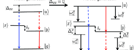
Figure 1: (Color online) Schematic of the resulting energy level diagram for cavity-QED assisted generation of entangled photons in the biexciton-exciton cascade decay after manipulating the binding energy of biexciton ($\Delta_{xx}\rightarrow 0$). The biexciton state $|u\rangle$ decays to the ground state $|g\rangle$ via intermediate exciton state $|x\rangle$ or $|y\rangle$, creating an $x-$polarized or $y-$polarized photons in the cavity modes. The $x-$polarized and $y-$polarized cavity modes are coupled with the $|u\rangle\rightarrow|x\rangle$, $|x\rangle\rightarrow|g\rangle$ and $|u\rangle\rightarrow|y\rangle$, $|y\rangle\rightarrow|g\rangle$ transitions, respectively.

An interesting alternate approach, insensitive to FSS, has been proposed recently, which suppressing the binding energy of the biexciton reimer ; avron ; tejedor . For a zero binding energy of the biexciton, photons of different polarizations match in energy in “across generations” (see Fig. 1). Because of the different ordering in the emission for $x-$polarized and $y-$polarized photon pairs, the photons are distinguishable temporarily and remain unentangled, but the entanglement can be restored using a time delay between photons of different generations.

The effects of dephasing in the generated entangled state of photons can be minimized significantly by enhancing the emission rates of photons through the Purcell effect in a system comprised of a QD coupled with a microcavity. Several experiments have also demonstrated single QD strong coupling to semiconductor cavities photocavity1 ; photocavity2 ; Peter2005 . Recently, Johne et al. johne proposed a cavity-QED scheme for generating entangled photons in the strong coupling regime. In their scheme, excitons are strongly coupled with cavity modes and form degenerate polariton states polariton . A formal theory of this scheme, including exciton and biexciton broadenings, has been reported by us ours . However, one drawback of the proposed scheme is that because of the large binding energy, the biexciton remains uncoupled with cavity modes and thus the first generation of photons has a long life time. In this paper, we propose a scheme for the fast generation of entangled photons from a single QD, by manipulating the binding energy of the biexciton such that both biexciton to excitons and excitons to ground state are coupled with two cavity modes of orthogonal polarization. Experimentally, manipulation of the binding energies of the biexciton has been reported by applying lateral electric field reimer and by thermal annealing annealing . In this proposed fast generation schemes introduced below, we discuss both “across generation” and “within generation” of entangled photons.

This paper is organized as follows. In Sec. II, we present a formal theory of a single QD coupled to a planar photonic cavity cavity. The cavity-assisted across generation of entangled photons is discussed in Sec. III. In Sec. IV, the cavity-assisted within generation of entangled photons is studies. In section V, we present our conclusions. In the appendix, we show a derivation for the dressed states of the biexciton.

II Theory

We consider a QD embedded in a photonic crystal (PC) cavity having two orthogonal polarization modes of frequencies $\omega_{c}^{x}$ and $\omega_{c}^{y}$, which can be realized and tuned experimentally using electron-beam lithography and, for example, AFM oxidization techniques HennessyAPL06 . The exciton states, $|x\rangle$ and $|y\rangle$, have FSS $\delta_{\rm x}$. The cavity modes are coupled with the biexciton to exciton and exciton to ground-state transitions, by manipulating the biexciton binding energy annealing ; reimer . The schematic arrangement of the system is shown in Fig. 1.

The Hamiltonian for the system of QD coupled with two-modes in PC-cavity, in the interaction picture, can be written as

$$\frac{H_{I}(t)}{\hbar} = g^{x}_{1}|x\rangle\langle g|\hat{a}_{c}^{x}e^{i\Delta_{c}^{x}t}+g^{x}_{2}|u\rangle\langle x|\hat{a}_{c}^{x}e^{i(\omega_{ux}-\omega_{c}^{x})t}+g^{y}_{1}|y\rangle\langle g|\hat{a}_{c}^{y}e^{i\Delta_{c}^{y}t}+g^{y}_{2}|u\rangle\langle y|\hat{a}_{c}^{y}e^{i(\omega_{uy}-\omega_{c}^{x})t}$$ (1)

$$+\sum_{m\neq c}\Omega_{xm}\hat{a}_{c}^{x{\dagger}}\hat{a}^{x}_{m}e^{i(\omega_{c}^{x}-\omega_{m})t}+\sum_{m\neq c}\Omega_{ym}\hat{a}_{c}^{y{\dagger}}\hat{a}^{y}_{m}e^{i(\omega_{c}^{y}-\omega_{m})t}+H.c.,\,$$

where $\omega_{ux}=\omega_{u}-\omega_{x}$, $\omega_{uy}=\omega_{u}-\omega_{y}$, $\Delta_{c}^{x}=\omega_{x}-\omega^{x}_{c}$, $\Delta_{c}^{y}=\omega_{y}-\omega_{c}^{y},$ and $\hat{a}^{i}_{j}$ are the field operators with $\hat{a}_{c}^{x}$ and $\hat{a}_{c}^{y}$ the cavity mode operators. Here, $\Omega_{xm}$, and $\Omega_{ym}$ represent the couplings to the environment from the cavity mode; $g^{i}_{j}$ are the coupling strength between the exciton/biexciton and cavity mode; $\omega_{m}^{i}$ are the frequencies of the $i-$polarized photons emitted from the cavity mode, and $\omega_{u}$, $\omega_{x}$, $\omega_{y}$ are the the frequency of the biexciton and excitons, respectively. We consider a system that is optically pumped in such a way as to have an initially-excited biexciton, with no photons inside the cavity, thus the state of the system at any time $t$ can be written as follows:

$$|\psi(t)\rangle = c_{1}(t)|u,0,0\rangle+c^{x}_{2}(t)|x,1,0\rangle+c^{y}_{2}(t)|y,0,1\rangle+c^{x}_{3}(t)|g,2,0\rangle+c^{y}_{3}(t)|g,0,2\rangle$$ (2)

$$+\sum_{m}c^{x}_{4m}(t)|x,0,0\rangle|1_{m}\rangle_{x}|0\rangle_{y}+\sum_{m}c^{y}_{4m}(t)|y,0,0\rangle|0\rangle_{x}|1_{m}\rangle_{y}+\sum_{m}c^{x}_{5m}(t)|g,1,0\rangle|1_{m}\rangle_{x}|0\rangle_{y}$$

$$+\sum_{m}c^{y}_{5m}(t)|g,0,1\rangle|0\rangle_{x}|1_{m}\rangle_{y}+\sum_{mn}c^{x}_{mn}(t)|g,0,0\rangle|1_{m},1_{n}\rangle_{x}|0\rangle_{y}+\sum_{mn}c^{y}_{mn}(t)|g,0,0\rangle|0\rangle_{x}|1_{m},1_{n}\rangle_{y}.\ \ \$$

The different terms in the state vector $|\psi\rangle$ represent, respectively: the dot is in the biexciton state with zero photons in the cavity; the dot is in the exciton state with one photon in the $x$-polarized cavity mode; the dot is in the exciton state with one photon in the $y$-polarized cavity mode; the dot is in ground state with two photon in $x$-polarized cavity mode; the dot is in the ground state with two photons in $y$-polarized cavity modes; and the additional possible terms due to leakage of photons from the cavity modes to the reservoirs; the suffixs to the reservoir kets represent their polarization.

By using the Schrödinger equation, applying the Weisskopf-Wigner approximation wwa ; raymer ; yao , and introducing biexciton and exciton broadenings, we derive the following equations of motion for the probability amplitudes:

$$\dot{c}_{1}(t) = -ig^{x}_{2}c^{x}_{2}(t)e^{i(\omega_{ux}-\omega_{c}^{x})t}-ig^{y}_{2}c^{y}_{2}(t)e^{i(\omega_{uy}-\omega_{c}^{y})t}$$ (3)

$$-\gamma_{1}c_{1}(t),$$

$$\dot{c^{\alpha}_{2}}(t) = -ig^{\alpha}_{2}c_{1}(t)e^{-i(\omega_{u\alpha}-\omega_{c}^{\alpha})t}-ig^{\alpha}_{1}\sqrt{2}\,c^{\alpha}_{3}(t)e^{i\Delta_{c}^{\alpha}t}$$ (4)

$$-\kappa c^{\alpha}_{2}(t)-\gamma_{2}c^{\alpha}_{2}(t),$$

$$\dot{c^{\alpha}_{3}}(t) = -ig^{\alpha}_{1}\sqrt{2}c^{\alpha}_{2}(t)e^{-i\Delta_{c}^{\alpha}t}-2\kappa c^{\alpha}_{3}(t),$$ (5)

$$\dot{c}^{\alpha}_{4m}(t) = -ig^{\alpha}_{1}c^{\alpha}_{5m}e^{i\Delta_{c}^{\alpha}t}-i\Omega_{\alpha m}^{*}c^{\alpha}_{2}e^{-i(\omega_{c}^{\alpha}-\omega_{m})t}$$ (6)

$$-\gamma_{2}c^{\alpha}_{4m}(t),$$

$$\dot{c}^{\alpha}_{5m}(t) = -ig^{\alpha}_{1}c^{\alpha}_{4m}e^{-i\Delta_{c}^{\alpha}t}-i\Omega_{\alpha m}^{*}\sqrt{2}\,c^{\alpha}_{3}(t)e^{-i(\omega_{c}^{\alpha}-\omega_{m})t}$$

$$-\kappa c^{\alpha}_{5m}(t),$$

$$\dot{c}^{\alpha}_{mn}(t) = -i\Omega_{\alpha n}^{*}c^{\alpha}_{5m}e^{-i(\omega_{c}^{\alpha}-\omega_{n})t},$$ (7)

where $\alpha=x$ or $y$, $\kappa=\pi|\Omega_{xm}|^{2}=\pi|\Omega_{ym}|^{2}$ is the half width of the cavity modes (assuming uniform and equal coupling for $x$ and $y$), and $\gamma_{1}$, $\gamma_{2}$ are the half widths of the biexciton and exciton levels, respectively. We note that $\gamma_{1}$ and $\gamma_{2}$ can include both radiative and nonradiative broadening, and for QDs, $\gamma_{1}\approx 2\gamma_{2}$. We next solve Eqs.(4)-(7) to obtain $c^{x}_{mn}$ and $c^{y}_{mn}$, using the Laplace transform method. The probability amplitudes for emission of a photon pair, in the long time limit, are

$$c^{x}_{mn}(\infty) = \frac{g^{x}_{1}\Omega^{*}_{xn}(\omega_{m}+3\omega_{n}-2\omega_{x}-2\omega_{c}^{x}+2i\kappa+2i\gamma_{2})}{(\omega_{n}-\omega_{x}+i\gamma_{2})(\omega_{n}-\omega_{c}^{x}+i\kappa)-(g^{x}_{1})^{2}}$$ (8)

$$\times\frac{g^{x}_{2}\Omega^{*}_{xm}F_{y}(\omega_{m},\omega_{n})}{D(\omega_{m},\omega_{n})},$$

$$c^{y}_{mn}(\infty) = \frac{g^{y}_{1}\Omega^{*}_{yn}(\omega_{m}+3\omega_{n}-2\omega_{y}-2\omega_{c}^{y}+2i\kappa+2i\gamma_{2})}{(\omega_{n}-\omega_{y}+i\gamma_{2})(\omega_{n}-\omega_{c}^{y}+i\kappa)-(g^{y}_{1})^{2}}$$ (9)

$$\times\frac{g^{y}_{2}\Omega^{*}_{ym}F_{x}(\omega_{m},\omega_{n})}{D(\omega_{m},\omega_{n})},$$

where

$$F_{\alpha}(\omega_{m},\omega_{n}) = 2(g^{\alpha}_{1})^{2}-(\omega_{m}+\omega_{n}-\omega_{\alpha}-\omega_{c}^{\alpha}+i\kappa+i\gamma_{2})$$ (10)

$$(\omega_{m}+\omega_{n}-2\omega_{c}^{\alpha}+2i\kappa),$$

$$D(\omega_{m},\omega_{n}) = (\omega_{m}+\omega_{n}-\omega_{u}+i\gamma_{1})F_{x}F_{y}$$ (11)

$$+(g^{x}_{2})^{2}F_{y}(\omega_{m}+\omega_{n}-2\omega_{c}^{x}+2i\kappa)$$

$$+(g^{y}_{2})^{2}F_{x}(\omega_{m}+\omega_{n}-2\omega_{c}^{y}+2i\kappa).$$

The optical spectrum of the generated $x$-polarized photon-pair is given by $S(\omega_{m},\omega_{n})=|c^{x}_{mn}(\infty)|^{2}$, and the spectrum for $y$-polarized photon pair is given by $S(\omega_{m},\omega_{n})=|c^{y}_{mn}(\infty)|^{2}$. The spectral functions, $S(\omega_{m},\omega_{n})$, represent the joint probability distribution, and thus the integration over the one frequency variable gives the spectrum at the other frequency. For example, the spectrum of the first generation of photons emitted via cavity mode is given by $S(\omega_{m})=\int_{-\infty}^{\infty}S(\omega_{m},\omega_{n})\,d\omega_{n}$, and the spectrum of second generation of photons is $S(\omega_{n})=\int_{-\infty}^{\infty}S(\omega_{m},\omega_{n})\,d\omega_{m}$.

From the above discussion, the state of the photon pair emitted from both the cavity modes is given by

$$|\psi\rangle=\sum_{m,n}c^{x}_{mn}(\infty)|1_{m},1_{n}\rangle_{x}+\sum_{m,n}c^{y}_{mn}(\infty)|1_{m},1_{n}\rangle_{y},$$ (12)

where in each term the ket represents the state of the cavity mode reservoirs, and the ket suffix labels the polarization. The coefficients $c^{\alpha}_{mn}(\infty)$ are given by the analytical expressions described through Eqs. (8) and (9).

III Cavity-assisted “across generation” of entangled photons

In the previous section, we have derived expressions for the final state of the photons generated in the biexciton-exciton cascade decay through leaky cavity modes. Depending on the coupling strength and detunings of the cavity modes from the transition frequencies in QD, the emitted $x-$polarized and $y-$polarized photons can match in energies within the same generations or through across generations. In this section we discuss the case when the photons match in energy in across generations. The state of the emitted photon pair is given by

$$|\psi\rangle=\sum_{k,l}[c^{x}_{kl}(\infty)|1_{k}\rangle_{x}|1_{l}\rangle_{x}+c^{y}_{lk}(\infty)|1_{l}\rangle_{y}|1_{k}\rangle_{y}],$$ (13)

where the first and second ket in each term show the photon of the first generation and the second generation, respectively; the second term corresponding to the $y-$polarized photon pair has the reverse ordering of indices compared to the first term. Although the photons of different polarizations in different generation could be degenerate in frequencies, they are distinguishable in order, namely in time. Thus, for generating entangled photons it is necessary to make photons temporally indistinguishable as well. For erasing the temporal information, photons of the first generation are delayed by time $t_{0}$. The normalized off-diagonal element of the density matrix of photons, in the polarization basis, is given by

$$\gamma=\frac{\int\int c^{x*}_{kl}(\infty)c^{y}_{lk}(\infty)W_{\rm opt}(\omega_{k},\omega_{l})\,d\omega_{k}d\omega_{l}}{\int\int|c^{x}_{kl}(\infty)|^{2}\,d\omega_{k}d\omega_{l}+|c^{y}_{lk}(\infty)|^{2}\,d\omega_{k}d\omega_{l}},$$ (14)

where $W_{\rm opt}=\exp[-i(\omega_{k}-\omega_{l})t_{0}]$ is an additional phase generated by the time delay. For $t_{0}=0$, i.e., no time delay is employed, $W_{\rm opt}=1$, and from Eq. (14) one gets $\gamma=0$. This shows that the phase $W_{\rm opt}$ is essential to erase the temporal information of photon emission from the state $\psi$ (Eq. 13). For a certain value of delay $t_{0}$, the photons of the first generation and second generations can become indistinguishable and the value of $|\gamma|$ has a maximum. We note that the concurrence wooters , which is a quantitative measure of entanglement, for the generated state of photons $|\psi\rangle$ is equal to $2|\gamma|$; so $|\gamma|=0.5$ represents the maximum entanglement.

In order to better understand the results for cavity-assisted generation of entangled photons we first consider the case when the QD is not coupled with the cavity modes. In that case, the photons are generated in the spontaneous emission through biexciton-exciton cascade decay avron , and the coefficients $c$ in Eq.(13) are given by

$$c^{x}_{kl}=\frac{\sqrt{\gamma_{1}\gamma_{2}/2\pi^{2}}}{(\omega_{k}+\omega_{l}-\omega_{u}+i\gamma_{1})(\omega_{l}-\omega_{x}+i\gamma_{2})},$$ (15)

$$c^{y}_{lk}=\frac{\sqrt{\gamma_{1}\gamma_{2}/2\pi^{2}}}{(\omega_{k}+\omega_{l}-\omega_{u}+i\gamma_{1})(\omega_{k}-\omega_{y}+i\gamma_{2})}.$$ (16)

For a QD having zero biexciton binding energy, i.e., $\omega_{u}=\omega_{x}+\omega_{y}$, and with a time delay $t_{0}$, from Eq. (14), one gets

$$\gamma=\frac{2\gamma_{2}e^{-2\gamma_{2}t_{0}}}{\gamma_{1}}(1-e^{-\gamma_{1}t_{0}}).$$ (17)

From Eq. (17), we notice that $\gamma$ is maximized for $\gamma_{2}t_{0}=\gamma_{2}\ln(1+\gamma_{1}/2\gamma_{2})/\gamma_{1}$. Normally for a QD, $\gamma_{1}/\gamma_{2}=2$, and the maximum value of $\gamma$ is 0.25; so after manipulating the decay such that $\gamma_{1}/\gamma_{2}\rightarrow 0$, the maximum value of $\gamma=1/e$ is obtained. Similar values have also been reported by simulating correlations within the density matrix formalism tejedor .

Figure 2: (color online) (a) Optimum value of $|\gamma|$ corresponding to a time delay $\gamma_{2}t_{0}=\gamma_{2}\ln(1+\gamma_{1}/2\gamma_{2})/\gamma_{1}$. (b) The value of $|\gamma|$ for $\gamma_{1}/\gamma_{2}=2$ (black) and for $\gamma_{1}/\gamma_{2}\rightarrow 0$ (blue).

It is important to note here, that the values of $|\gamma|$ using a time delay are quite different to the values reported by Avron et. al. avron . The reason for this discrepancy, is that we have considered an experimentally feasible linear time delay, while Avron et al. considered a complex nonlinear time delay that is practically impossible to realize comment . Consequently, the maximum value of concurrence in across generation of entangled photons through time reordering is 0.73, even after optimally manipulating the exciton/biexciton line widths. In Fig. 2(a) we show the dependence of entanglement on the value of $\gamma_{1}/\gamma_{2}$. The dependence of the off-diagonal element of of photon density matrix on delay time is shown in Fig. 2(b). For QDs, $\gamma_{1}$ and $\gamma_{2}$ have radiative and non-radiative parts, and generally the nonradiative parts are larger than the radiative parts. Thus it is not possible to manipulate the values of $\gamma_{1}/\gamma_{2}$ significantly by changing the decay rates of the biexciton and excitons dotsize . However, in the coupld QD - PC cavity system, the radiative halfwidths of biexciton and excitons can be significantly larger than their nonradiative half widths, and by tuning the cavity mode frequencies and couplings parameters one can manipulate the ratio of the biexciton line width to the exciton line width and thus increase the degree of entanglement. Also, the required delay time for maximizing the entanglement can be achieved by creating path differences for photons of selected polarization and frequency. For smaller values of $\gamma_{2}$, one must generate a large optical path difference between photons to realize the appropriate time delays $t_{0}$, corresponding to $\gamma_{2}t_{0}=\gamma_{2}\ln(1+\gamma_{1}/2\gamma_{2})/\gamma_{1}$. However, for a QD coupled with a cavity, the decay rates of the biexciton and exciton could be very large, thus the required delay time will be significantly small and can be achieved easily in an appropriate optical delay scheme avron .

For across generation of entangled photons, we consider a QD coupled with a PC-cavity when the binding energy of biexciton is suppressed to zero. We plot values of $|\gamma|$ for typical values of cavity couplings and detunings in Fig. 3. For the weak coupling regime, the radiative decay rates of the exciton states via the cavity modes are given by $\Gamma^{i}_{2}=g^{i~{}2}_{1}\kappa/(\kappa^{2}+\Delta^{i~{}2}_{c})$, for $i=x,y$. The radiative decay rates for the biexciton state $|u\rangle$ into the exciton states $|x\rangle$ and $|y\rangle$ are given by $\Gamma^{x}_{1}=g^{x~{}2}_{2}\kappa/[\kappa^{2}+(\Delta^{x}_{c}-\delta_{x})^{2}]$ and $\Gamma^{y}_{1}=g^{y~{}2}_{2}\kappa/[\kappa^{2}+(\Delta^{y}_{c}+\delta_{x})^{2}]$. The value of $|\gamma|$ is larger when the biexciton decay rates into both exciton states are equal, i.e., $\Gamma^{x}_{1}=\Gamma^{y}_{1}$. For positive $\delta_{x}=\omega_{x}-\omega_{y}$, if we choose $\Delta_{c}^{x}$ negative and $\Delta_{c}^{y}$ positive, the transition $|u\rangle\rightarrow|x\rangle$ and $|u\rangle\rightarrow|y\rangle$ will be detuned with cavity modes by $-(\Delta_{c}^{x}+\delta_{x})$ and $\Delta_{c}^{y}+\delta_{x}$. Because of the larger detunings, the decay rates of the biexciton states becomes smaller which enhances the entanglement between the generated photons. In addition, the ratio $\Gamma^{x}_{1}/\Gamma^{x}_{2}$ and $\Gamma^{y}_{1}/\Gamma^{y}_{2}$ is a maximum for cavity mode frequencies resonant with the excitons, i.e. $\Delta^{x}_{c}=\Delta^{y}_{c}=0$, and for larger values of $\delta_{x}$. In Figs. 3(a,c), the cavity modes are resonant with the exciton frequencies and interact with the QD in the weak coupling regime. The maximum possible values of $|\gamma|$ is nearly 0.35 (Fig. 3(c)) which is close to the theoretical maximum value of 0.367. For the strong coupling regime, the two frequencies of photons in each polarization become inseparable for small detunings. However, for larger detunings, when the photons are spectrally well resolved (see Figs. 3(b,d)), the decay rates of the biexciton to excitons and the excitons to the ground state remains nearly the same and the value of $|\gamma|$ is around 0.25.

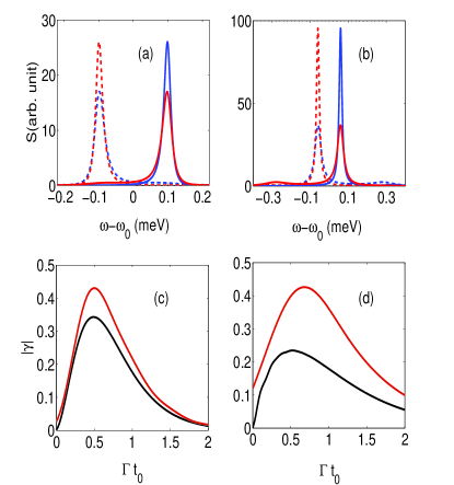
Figure 3: (Color online) The “across generation” of entangled photons when biexciton is also coupled with cavity modes after reducing binding energy $\Delta_{xx}=0$ meV. On the left, we consider weak coupling with the cavity modes degenerate with the exciton modes, and on the right we consider strong coupling with the cavity modes detuned with respect to the exciton modes. The spectrum of the photons $S(\omega)$ for $\delta_{x}=0.2$ meV, $\gamma_{1}=2\gamma_{2}=0.004\,$meV, $\kappa=0.05$ meV, for (a) $g^{x}_{1}=g^{x}_{2}=g^{y}_{1}=g^{y}_{2}=0.02$ meV, and $\Delta_{c}^{x}=\Delta_{c}^{y}=0$ meV, and for (b) $g^{x}_{1}=g^{x}_{2}=g^{y}_{1}=g^{y}_{2}=0.1$ meV, and $\Delta_{c}^{x}=-\Delta_{c}^{y}=-0.2$ meV. The $x-$polarized photons are shown in blue and the $y-$polarized are shown in red; also, the solid curves are for photons generated in the exciton decay and the dotted curves are for photons generated in the biexciton decay. (c-d) The values of $|\gamma|$ corresponding to time delay $\Gamma t_{0}$, where $\Gamma=g^{2}\kappa/(\kappa^{2}+\Delta_{c}^{x2})$. The red (black) curves represent results for filtered (unfiltered) photons. For (c) the filter function corresponds to two spectral windows of width $w=0.05\,$ meV, centered at $\omega_{x}$ and $\omega_{y}$, and for (d) the filter function corresponds to two spectral windows of width $w=0.03\,$ meV, centered at $\omega_{x}^{-}$ and $\omega_{y}^{+}$.

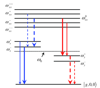
Figure 4: (color online) The dressed states of biexciton and exciton for across generation of entangled photons. The upper five states $\omega_{xx}^{i}$ are the dressed state of the biexciton and the lower states $\omega_{x}^{i}$, $\omega_{y}^{i}$ are the dressed state of the $|x\rangle$ and $|y\rangle$ excitons, respectively. The bold arrows corresponding to the dominating peaks in the emitted spectrum.

To better understand the physical origin of the spectrum of Fig. 3(b), we have analytically calculated the dressed states of the biexciton and excitons in the rotating frame with frequency $\omega_{0}$, in the strong coupling regime. We relegate the details of the calculation to the appendix. For an initial state $|u,0,0\rangle$, the coupled cavity-QD system has five dressed states that can be expressed as the orthonormal superpositions of the bare states $|u,0,0\rangle$, $|x,1,0\rangle$, $|y,0,1\rangle$, $|g,2,0\rangle$, and $|g,0,2\rangle$. For $\Delta_{c}^{x}=-\Delta_{c}^{y}=\Delta$, $g_{1}^{x}=g_{1}^{y}=g_{1}$, and $g_{2}^{x}=g_{2}^{y}=g_{2}$, the energies of these biexciton dressed states are given by $\omega_{xx}^{0}=0$, $\omega_{xx}^{\pm}=\pm\sqrt{A-B}$, and $\omega_{xx}^{\pm\pm}=\pm\sqrt{A+B}$, where $A=[4g_{2}^{2}+(2\delta_{x}-3\Delta)^{2}+\Delta^{2}+8g_{1}^{2}]/4$, and $B=\sqrt{[2g_{2}^{2}+\Delta(2\delta_{x}-3\Delta)]^{2}+8g_{1}^{2}(2\delta_{x}-3\Delta)^{2}}/2$. After emitting the first photon via the leaky cavity mode, the system jumps to the dressed states of the excitons, which are superposition of either $|x,0,0\rangle$ and $|g,1,0\rangle$ or $|y,0,1\rangle$ and $|g,0,1\rangle$, depending on whether the emitted photon was $x-$polarized or $y-$polarized, respectively. The frequencies of the exciton dressed states are given by $\omega_{x}^{\pm}=(\delta_{x}-\Delta\pm\sqrt{4g_{1}^{2}+\Delta^{2}})/2$, $\omega_{y}^{\pm}=(-\delta_{x}+\Delta\pm\sqrt{4g_{1}^{2}+\Delta^{2}})/2$. In principle, the first emitted photon from the dressed states of biexciton can have ten peaks in the spectrum; however, for the initial state $|u,0,0\rangle$ and an off-resonant leaky cavity modes, only two peaks appear in the spectrum corresponding to $\omega_{xx}^{0}\rightarrow\omega_{x}^{-}$ and $\omega_{xx}^{+}\rightarrow\omega_{x}^{-}$ for $x-$polarized and $\omega_{xx}^{0}\rightarrow\omega_{y}^{+}$ and $\omega_{xx}^{-}\rightarrow\omega_{y}^{+}$ for $y-$polarization; other possible transitions are negligible (see Fig. 4). Further, the peaks corresponding to $\omega_{xx}^{0}\rightarrow\omega_{x}^{-}$ and $\omega_{xx}^{0}\rightarrow\omega_{y}^{+}$ dominate completely. The second photon is emitted from the decay of the dressed states of excitons and have a two-peak spectrum corresponding to frequencies $\omega_{x}^{\pm}$ or $\omega_{y}^{\pm}$. The peaks corresponding to frequencies $\omega_{x}^{-}$ for the $x-$polarized photon and $\omega_{y}^{+}$ for the $y-$polarized photon are largely dominating.

Although the value of $|\gamma|$ is limited by $2/e$ in across generation of photons through time delay, nevertheless, the entanglement can be distilled by using a frequency filter having two narrow spectral windows of width $w$ centered at the frequencies of degenerate peaks in the spectrum of $x-$polarized and $y-$polarized photons, say, $\omega_{1}$ and $\omega_{2}$. Subsequently, the response of the spectral filter can be written as a projection operator of the following form

$$F(\omega_{k},\omega_{l})=\left\{\begin{array}[]{cc}1,&{\rm for}~{}|\omega_{k}-\omega_{1}|<w,\\ 1,&{\rm for}~{}|\omega_{l}-\omega_{2}|<w,{}{}{}{}{}{}{}{}{}\\ 0,&{\rm otherwise.{}{}{}{}{}{}{}{}{}{}{}{}{}{}{}{}{}}\end{array}\right.$$ (21)

After operating on the wave function of the emitted photons (Eq. (12)), by the spectral function $F(\omega_{k},\omega_{l})$ and tracing over the energy states akopian , we get the reduced density matrix of the filtered photon pairs in the polarization basis. The normalized off-diagonal element of the density matrix for filtered photons $\gamma$ can be computed by integrating over the projection operator of the filter akopian . One has

$$\gamma=\frac{\int\int c^{x*}_{kl}c^{y}_{lk}W_{opt}(\omega_{k},\omega_{l})F(\omega_{k},\omega_{l})d\omega_{k}d\omega_{l}}{\int\int\left[|c^{x}_{kl}|^{2}F(\omega_{k},\omega_{l})+|c^{y}_{lk}|^{2}F(\omega_{k},\omega_{l})\right]d\omega_{k}d\omega_{l}}.$$ (22)

We show in Figs. 3(c,d) (red curves) that large values of $|\gamma|$ can be achieved by using a spectral filter. The higher values of $|\gamma|$ are achieved because of the fact that the photons along the tails in the spectrum do not get time reordered properly using a linear time delay and thus reduce the entanglement. We find that the entanglement can be distilled by using a frequency filter with two spectral windows centered at the frequencies $\omega_{x}$ and $\omega_{y}$ for the weakly coupling case and $\omega_{x}^{-}$ and $\omega_{y}^{+}$ for the strong coupling case. Again it should be noted that the conditional probabilities after filtering, for generating entangled photon pairs, are very large (80% for Fig. 3(c) and 50% for Fig. 3(d)) because of the fact that photons are selected around the degenerate spectral peaks not along the degenerate tails as performed in earlier works akopian , where the conditional probabilities are much less (e.g., less than 5% conditional probabilities for 80% concurrence values).

IV “Within generation” of entangled photons

For within generation of entangled photons, the $x-$polarized and $y-$polarized photons should match in energy within the same generations. In this case we consider the exciton states, which have a small but non-zero FSS, to interact with cavity modes in strong coupling regime so that the system forms degenerate polariton states johne ; ours . Here we extend previous works johne ; ours by considering that the biexciton state is also coupled with the same cavity modes by reducing the binding energy; however, the biexciton to exciton transition is more off-resonant so that further splitting in the polariton states due to biexciton couplings is negligible.

The state of the photon pair emitted via cavity modes can be rewritten as

$$|\psi\rangle=\sum_{k,l}[c^{x}_{kl}(\infty)|1_{k}\rangle_{x}|1_{l}\rangle_{x}+c^{y}_{kl}(\infty)|1_{k}\rangle_{y}|1_{l}\rangle_{y}],$$ (23)

The coefficients $c$ are given by the previously calculated Eqs. (8)-(9). For state (23), the off-diagonal density matrix elements in the polarization basis is written as

$$\gamma=\frac{\int\int c^{x*}_{kl}(\infty)c^{y}_{kl}(\infty)\,d\omega_{k}d\omega_{l}}{\int\int|c^{x}_{kl}(\infty)|^{2}\,d\omega_{k}d\omega_{l}+|c^{y}_{lk}(\infty)|^{2}\,d\omega_{k}d\omega_{l}}.$$ (24)

We consider a positive detuning $\Delta_{c}^{x}$ and a negative detuning $\Delta_{c}^{y}$, which are equal to the FSS, i.e., $\Delta_{c}^{x}=-\Delta_{c}^{y}=\delta_{x}$. In this case, the biexciton to exciton transition $|u\rangle\rightarrow|x\rangle$ and $|u\rangle\rightarrow|y\rangle$ are equally detuned by $-\Delta_{xx}$. The exciton coupled with cavity modes form degenerate polariton states for $\Delta_{c}^{x}=-\Delta_{c}^{y}=\delta_{x}$. It should be noted here that although the biexciton is more detuned, still the decay rate of biexciton via cavity modes could be much larger than $\gamma_{1}$ (sum of radiative and nonradiative half width in free space).

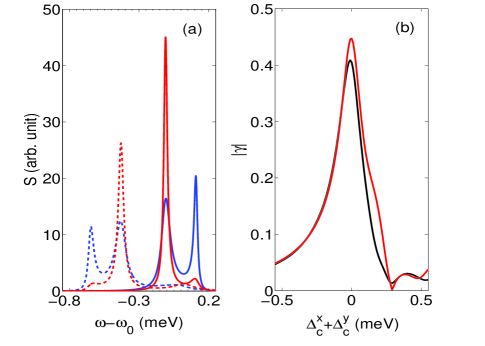
Figure 5: (Color online) The “within generation” of entangled photons when the biexciton is also coupled with the cavity modes; the biexciton binding energy is reduced to $\Delta_{xx}=0.5$ meV. (a) The spectrum of the photons $S(\omega)$ for $\delta_{x}=0.1$ meV, $\gamma_{1}=2\gamma_{2}=0.004\,$meV, $\kappa=0.05$ meV, $g^{x}_{1}=g^{x}_{2}=g^{y}_{1}=g^{y}_{2}=g=0.1$ meV, and $\Delta_{c}^{x}=-\Delta_{c}^{y}=0.1$ meV . The $x-$polarized photons are shown in blue and the $y-$polarized are shown in red; also, the solid curves are for photons generated in the exciton decay and the dotted curves are for photons generated in the biexciton decay. (b) The values of $|\gamma|$ for generated photons, by changing $\Delta_{c}^{x}$ for $\Delta_{c}^{y}=-0.1$ meV. The red (black) curve represents the results for filtered (unfiltered) photons; the filter function corresponds to two spectral windows of width $w=0.15\,$ meV, centered at $\omega-\omega_{0}=-0.45$ meV and $\omega-\omega_{0}=-0.05$ meV.

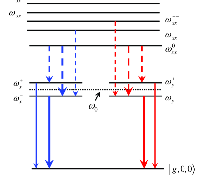
Figure 6: (color online) Same as in Fig. 4, but for within generation of entangled photons.

In Fig. 5(a), we show the spectrum of the photons generated in first generation (dotted lines) and in the second generation (solid line). It is necessary that the first generation and the second generation photons should be well resolved spectrally, therefore a moderate ($\sim 2\sqrt{4g_{1}^{x~{}2}+\delta_{x}^{2}}$) binding energy of the biexciton is essential for the within generation scheme of entangled photons. In this case, for $\Delta_{c}^{x}=-\Delta_{c}^{y}=\delta_{x}$, $g_{1}^{x}=g_{1}^{y}=g_{1}$, $g_{2}^{x}=g_{2}^{y}=g_{2}$, and $\Delta_{xx}\gg g_{2}$, we find that the dressed states of biexciton are given by (see appendix)

$$\omega_{xx}^{0} \approx -\left(\Delta_{xx}+\frac{2g_{2}^{2}}{\Delta_{xx}}\right),$$ (25)

$$\omega_{xx}^{+} \approx \epsilon^{+}+\frac{g_{2}^{2}\cos^{2}\theta}{\Delta_{xx}+\epsilon^{+}},$$ (26)

$$\omega_{xx}^{-} \approx \epsilon^{-}+\frac{g_{2}^{2}\sin^{2}\theta}{\Delta_{xx}+\epsilon^{-}},$$ (27)

$$\omega_{xx}^{++} \approx -\epsilon^{-}+\frac{g_{2}^{2}\sin^{2}\theta}{\Delta_{xx}-\epsilon^{-}},$$ (28)

$$\omega_{xx}^{--} \approx -\epsilon^{+}+\frac{g_{2}^{2}\cos^{2}\theta}{\Delta_{xx}-\epsilon^{+}},$$ (29)

where $\epsilon_{\pm}=(-\delta_{x}\pm\sqrt{\delta_{x}^{2}+8g_{1}^{2}})/2$, and $\theta=\tan^{-1}[2\sqrt{2}g_{1}/(\delta_{x}+\sqrt{\delta_{x}^{2}+8g_{1}^{2}})]$. Using the parameters of Fig. 5, $\omega_{xx}^{0}=-0.54$ meV, $\omega_{xx}^{+}=0.11$ meV, $\omega_{xx}^{-}=-0.19$ meV, $\omega_{xx}^{++}=0.20$ meV, $\omega_{xx}^{--}=-0.08\,$meV, and the dressed states of exciton are given by $\omega_{x}^{\pm}=\omega_{y}^{\pm}=\pm(4g_{1}^{2}+\delta_{x}^{2})/2=\pm 0.11$. Both exciton states for different polarization becomes degenerate for $\Delta_{c}^{x}=-\Delta_{c}^{y}=\delta_{x}$ johne ; ours . The schematic diagram of the dressed states is shown in Fig.6. The spectra of the first generation photons, mostly generated in the decay of biexciton dressed state $\omega_{xx}^{0}$, have two pronounced peaks corresponding to the frequencies $\omega_{xx}^{0}-\omega^{\pm}_{x}$, i.e., at -0.65 meV and -0.43 meV in Fig. 5; there is a very small probability for generation of photons in the transitions $\omega_{xx}^{-}\rightarrow\omega_{x}^{-}$ and $\omega_{xx}^{--}\rightarrow\omega_{y}^{-}$ corresponding to frequencies -0.08 meV, 0.03 meV, respectively. The spectra of photons in the second generation have two peaks corresponding to dressed state of excitons at $\pm 0.11$ meV.

The calculated value of $|\gamma|$ is shown in Fig. 5(b). For tuning the cavity mode frequencies, we fix one of the detunings $\Delta_{c}^{x}$ and $\Delta_{c}^{y}$, and change the other. This type of tuning has been experimentally shown using AFM oxidization techniques HennessyAPL06 , and note note that this scheme would be suitable to tune a large number of cavity-QD systems on the same chip. For this within generation study, we find very large values of $|\gamma|$ for the deterministic generation of photons. For further distilling the entanglement, spectral filters can also be used, but with a reduced probability and efficiency. Using spectral filtering, the maximally entangled photons can be generated with a small reduction of probability of detection. We show the results for spectrally filtered photons in Fig. 5(b) by the red curve. The values of $|\gamma|$ are calculated using Eq.(24) after multiplying with the filter function (Eq. 21).

V Conclusions

In summary, we have presented methods for across generation and within generation of entangle photons using single QD coupled with a PC-cavity, and exploited the fact that the biexciton binding energy can be tuned. For zero biexciton binding energy, the concurrence for the across generation through time delay of photons is limited by 2/e, which can be enhanced to 1 using a spectral filter, at the expense of reduced probability. For small biexciton binding energies, the system can be tuned for efficient within generation of entangled photons. The concurrence larger than 0.8 has been shown for within generation of fast entangled photons, even without spectral filtering.

Appendix A Dressed states of the biexciton

The Hamiltonian for the system of the QD coupled with two-modes in PC-cavity, in the rotating frame with frequency $\omega_{0}=(\omega_{x}+\omega_{y})/2$, for $\Delta_{c}^{x}=-\Delta_{c}^{y}=\Delta$, $g_{1}^{x}=g_{1}^{y}=g_{1}$, and $g_{2}^{x}=g_{2}^{y}=g_{2}$, and neglecting the coupling with environment, can be written as

$$\frac{H_{R}}{\hbar} = -\Delta_{xx}|u\rangle\langle u|+\frac{\delta_{x}}{2}\left(|x\rangle\langle x|-|y\rangle\langle y|\right)$$ (30)

$$-\left(\Delta-\frac{\delta_{x}}{2}\right)\hat{a}_{c}^{x{\dagger}}\hat{a}_{c}^{x}+\left(\Delta-\frac{\delta_{x}}{2}\right)\hat{a}_{c}^{y{\dagger}}\hat{a}_{c}^{y}$$

$$+[g_{1}|x\rangle\langle g|\hat{a}_{c}^{x}+g_{2}|u\rangle\langle x|\hat{a}_{c}^{x}+g_{1}|y\rangle$$

$$\langle g|\hat{a}_{c}^{y}+g_{2}|u\rangle\langle y|\hat{a}_{c}^{y}+H.c.].$$

For the across generation of entangled photons, $\Delta_{xx}=0$, we diagonalize the Hamiltonian and find the dressed energy states of the biexciton as follows

$$\omega_{xx}^{0}=0,$$ (31)

$$\omega_{xx}^{+}=\sqrt{A-B},$$ (32)

$$\omega_{xx}^{-}=-\sqrt{A-B},$$ (33)

$$\omega_{xx}^{++}=\sqrt{A+B},$$ (34)

$$\omega_{xx}^{--}=-\sqrt{A+B},$$ (35)

with

$$A=\frac{1}{4}[4g_{2}^{2}+(2\delta_{x}-3\Delta)^{2}+\Delta^{2}+8g_{1}^{2}]$$

$$B=\frac{1}{2}\sqrt{[2g_{2}^{2}+\Delta(2\delta_{x}-3\Delta)]^{2}+8g_{1}^{2}(2\delta_{x}-3\Delta)^{2}}.$$

For within generation of entangled photons, $\Delta_{xx}\neq 0$ and $\Delta=\delta_{x}$, from Eq.(30) we can rewrite the Hamiltonian $H_{R}$, in the basis of the state of the combined QD-cavity system as follows

$$H_{R} = -\hbar\Delta_{xx}|u,0,0\rangle\langle u,0,0|+\hbar g_{2}\left[|u,0,0\rangle\langle x,1,0|\right.$$ (37)

$$\left.+|u,0,0\rangle\langle y,0,1|+H.c.\right]+H_{S},$$

$$H_{S} = -\hbar\delta_{x}\left(|g,2,0\rangle\langle g,2,0|-|g,0,2\rangle\langle g,0,2|\right)$$ (38)

$$+\hbar g_{1}\sqrt{2}\left[|x,1,0\rangle\langle g,2,0|+|y,0,1\rangle\langle g,0,2|\right.$$

$$\left.+H.c.\right].$$

After diagonalizing $H_{S}$, the eigenstates and corresponding eigenvalues of $H_{S}$ are given by

$$|x_{+}\rangle = \cos\theta|x,1,0\rangle+\sin\theta|g,2,0\rangle,~{}~{}~{}~{}~{}\epsilon_{+}$$ (39)

$$|x_{-}\rangle = -\sin\theta|x,1,0\rangle+\cos\theta|g,2,0\rangle,~{}~{}\epsilon_{-}$$ (40)

$$|y_{+}\rangle = \sin\theta|y,0,1\rangle+\cos\theta|g,0,2\rangle,~{}~{}-\epsilon_{-}$$ (41)

$$|y_{-}\rangle = \cos\theta|y,0,1\rangle-\sin\theta|g,0,2\rangle,~{}~{}-\epsilon_{+},$$ (42)

where $\epsilon_{\pm}=(-\delta_{x}\pm\sqrt{\delta_{x}^{2}+8g_{1}^{2}})/2$, and $\theta=\tan^{-1}[2\sqrt{2}g_{1}/(\delta_{x}+\sqrt{\delta_{x}^{2}+8g_{1}^{2}})]$. We can rewrite the Hamiltonian $H_{0}$ in terms of eigenstates of $H_{s}$ as follows

$$H_{0} = -\hbar\Delta_{xx}|u\rangle\langle u|+\hbar\epsilon^{+}(|x_{+}\rangle\langle x_{+}|-|y_{-}\rangle\langle y_{-}|)$$ (43)

$$+\hbar\epsilon^{-}(|x_{-}\rangle\langle x_{-}|-|y_{+}\rangle\langle y_{+}|)$$

$$+\hbar g_{2}\cos\theta\left[|u\rangle\langle x_{+}|+|u\rangle\langle y_{-}|+H.c\right]$$

$$-\hbar g_{2}\sin\theta\left[|u\rangle\langle x_{-}|-|u\rangle\langle y_{+}|+H.c\right].$$

For $\Delta_{xx}>>g_{2}$, we can use perturbation theory and obtain the frequency eigenvalues

$$\omega_{xx}^{0} = -\Delta_{xx}-2\Delta_{xx}\left(\frac{g_{2}^{2}\cos^{2}\theta}{\Delta_{xx}^{2}-\epsilon^{+2}}+\frac{g_{2}^{2}\sin^{2}\theta}{\Delta_{xx}^{2}-\epsilon^{-2}}\right),$$ (44)

$$\approx -\left(\Delta_{xx}+\frac{2g_{2}^{2}}{\Delta_{xx}}\right),$$

$$\omega_{xx}^{+} = \epsilon^{+}+\frac{g_{2}^{2}\cos^{2}\theta}{\Delta_{xx}+\epsilon^{+}},$$ (45)

$$\omega_{xx}^{-} = \epsilon^{-}+\frac{g_{2}^{2}\sin^{2}\theta}{\Delta_{xx}+\epsilon^{-}},$$ (46)

$$\omega_{xx}^{++} = -\epsilon^{-}+\frac{g_{2}^{2}\sin^{2}\theta}{\Delta_{xx}-\epsilon^{-}},$$ (47)

$$\omega_{xx}^{--} = -\epsilon^{+}+\frac{g_{2}^{2}\cos^{2}\theta}{\Delta_{xx}-\epsilon^{+}}.$$ (48)

References

- (1) E. Knill, R. Laflamme and G. J. Milburn, Nature(London) 409, 46 (2001).
- (2) J. L. O’Brien, G. J. Pryde, A. G. White, T. C. Ralph, and D. Branning, Nature (London) 426, 264 (2003).
- (3) T. Jennewein, C. Simon, G. Weihs, H. Weinfurter, and A. Zeilinger, Phys. Rev. Lett. 84, 4729 (2000); D. S. Naik, C. G. Peterson, A. G. White, A. J. Berglund, and P. G. Kwiat, ibid. 84, 4733 (2000).
- (4) D. Bouwmeester, J.-W. Pan, K. Mattle, M. Eibl, H. Weinfurter, A. Zeilinger, Nature (London) 390, 575 (1997); D. Boschi, S. Branca, F. De Martini, L. Hardy, and S. Popescu, Phys. Rev. Lett. 80, 1121 (1998).
- (5) L. Mandel and E. Wolf, Optical Coherence and Quantum Optics (Cambridge University Press, Cambridge, England, 1995).
- (6) P. G. Kwiat, K. Mattle, H. Weinfurter, A. Zeilinger, A. V. Sergienko, and Y. Shih, Phys. Rev. Lett. 75, 4337 (1995).
- (7) P. Zoller, Th. Beth, D. Binosi, R. Blatt, H. J. Briegel, D. Bruss, T. Calarco, J. I. Cirac, D. Deutsch, J. Eisert, A. Ekert, C. Fabre, N. Gisin, P. Grangiere, M. Grassl, S. Haroche, A. Imamoglu, A. Karlson, J. Kempe, L. Kouwenhoven, S. Kr ll, G. Leuchs, M. Lewenstein, D. Loss, N. L tkenhaus, S. Massar, J.E. Mooij, M. B. Plenio, E. S. Polzik, S. Popescu, G. Rempe, A. Sergienko, D. Suter, J. Twamley, G. Wendin, R. Werner, A. Winter, J. Wrachtrup, A. Zeilinger, Eur. Phys. J. D 36/2, 203 (2005).
- (8) N. Akopian, N. H. Lindner, E. Poem, Y. Berlatzky, J. Avron, D. Gershoni, B. D. Gerardot, and P. M. Petroff, Phys. Rev. lett 96, 130501 (2006).
- (9) R. M. Stevenson, R. J. Young, P. Atkinson, K. Cooper, D. A. Ritchie, and A. J. Shields, Nature (London) 439, 179 (2006); R. M. Stevenson, R. J. Young, P. See, D. G. Gevaux, K. Cooper, P. Atkinson, I. Farrer, D. A. Ritchie, and A. J. Shields, Phys. Rev. B 73, 033306 (2006); K. Kowalik, O. Krebs, A. Golnik, J. Suffczyn’ski, P. Wojnar, J. Kossut, J. A. Gaj, and P. Voisin, Phys. Rev. B 75, 195340 (2007).
- (10) B. D. Gerardot, S. Seidl, P. A. Daigarno, R. J. Warburton, D. Granados, J. M. Garcia, K. Kowalik, and O. Krebs, Appl. Phys. Lett. 90, 041101 (2007); M. M. Vogel, S. M. Ulrich, R. Hafenbrak, P. Michler, L. Wang, A. Rastelli, and O. G. Schmidt, Appl. Phys. Lett. 91, 051904 (2007).
- (11) R. Seguin, S. Schliwa, T. D. Germann, S. Rodt, K. P tschke, A. Strittmatter, U. W. Pohl, D. Bimberg, M. Winkelnkemper, T. Hammerschimidt, and P. Kratzer, Appl. Phys. Lett. 89, 263109 (2006); D. J. P. Ellis, R. M. Stevenson, R. J. Young, A. J. Shields, P. Atkinson, and D. A. Ritchie, ibid. 90, 011907 (2007).
- (12) R. Hafenbrak, S. M. Ulrich, P. Michler, L. Wang, A. Rastelli and O. G. Schmidt, New J. Phys. 9, 315 (2007).
- (13) R. M. Stevenson, A. J. Hudson, A. J. Bennett, R. J. Young, C. A. Nicoll, D. A. Ritchie, and A. J. Shields, Phys. Rev. Lett. 101, 170501 (2008); R. J. Young, R. M. Stevenson, A. J. Hudson, C. A. Nicoll, D. A. Ritchie, and A. J. Shields, Phys. Rev. Lett. 102, 030406 (2009).
- (14) U. Hohenester, G. Pfanner, and M. Seliger, Phys. Rev. Lett. 99, 047402 (2007).
- (15) A. J. Hudson, R. M. Stevenson, A. J. Bennett, R. J. Young, C. A. Nicoll, P. Atkinson, K. Cooper, D. A. Ritchie, and A. J. Shields, Phys. Rev. Lett. 99, 266802 (2007).
- (16) F. P. Laussy, E. delValle, and C. Tejedor, Phys. Rev. Lett. 101, 083601 (2008).
- (17) D. Gammon, E. S. Snow, B. V. Shanabrook, D. S. Katzer, and D. Park, Phys. Rev. Lett. 76, 3005 (1996).
- (18) M. E. Reimer, M. Korkusin’ski, D. Dalacu, J. Lefebvre, J. Lapointe, P. J. Poole, G. C. Aers, W. R. McKinnon, P. Hawrylak, and R. L. Williams, Phys. Rev. B 78, 195301 (2008); M. Korkusinski, M. E. Reimer, R. L. Williams, and P. Hawrylak, Phys. Rev. B 79, 035309 (2009).
- (19) J. E. Avron, G. Bisker, D. Gershoni, N. H. Lindner, E. A. Meirom, and R. J. Warburton, Phys. Rev. Lett. 100, 120501 (2008).
- (20) F. Troiani and C. Tejedor, Phys. Rev. B 78, 155305 (2008).
- (21) J. P. Reithmaier, G. Sek, A. Löffler, C. Hofmann, S. Kuhn, S. Reitzenstein, L. V. Keldysh, V. D. Kulakovskii, T. L. Reinecke and A. Forchel, Nature (London) 432, 197 (2004).
- (22) T. Yoshie, A. Scherer, J. Hendrickson, G. Khitrova, H. M. Gibbs, G. Rupper, C. Ell, O. B. Shchekin, and D. G. Deppe, Nature (London) 432, 200 (2004).
- (23) E. Peter, P. Senellart, D. Martrou, A. Lemaitre, J. Hours, J. M. Gérard, and J. Bloch, Phys. Rev. Lett., 95, 067401 (2005).
- (24) R. Johne, N. A Gippius, G. Pavlovic, D. D. Solnyshkov, I. A. Shelykh, and G. Malpuech, Phys. Rev. lett. 100, 240404 (2008).
- (25) G. Jundt, L. Robledo, A. Hogele, S. Falt, and A. Imamoglu, Phys. Rev. Lett. 100, 177401 (2008).
- (26) P. K. Pathak and S. Hughes, Phys. Rev. B 79, 205416 (2009).
- (27) K. Hennessy, C. Hogerle, E. Hu, A. Badolato, and A. Imamoglu, Appl. Phys. Lett. 89, 041118 (2006).
- (28) M. M. Ashraf, Phys. Rev. A 50, 741 (1994).
- (29) V. Weisskopf and E. Wigner, Z. Phys. 63, 54 (1930).
- (30) G. Cui and M. G. Raymer, Phys. Rev. A 73, 053807 (2006).
- (31) S. Hughes and P. Yao, Optics Express 17, 3322 (2009).
- (32) W. K. Wooters, Phys. Rev. Lett. 80, 2245 (1998).
- (33) P. K. Pathak and S. Hughes, submitted; see arXiv:0905.4420v1 [cond-mat.mes-hall]
- (34) M. Wimmer, S. V. Nair, and J. Shumway, Phys. Rev. B 73, 165305 (2006).