On the density of the sum of two independent Student t-random vectors

Abstract

In this paper, we find an expression for the density of the sum of two independent $d-$dimensional Student $t-$random vectors $\mathbf{X}$ and $\mathbf{Y}$ with arbitrary degrees of freedom. As a byproduct we also obtain an expression for the density of the sum $\mathbf{N}+\mathbf{X}$, where $\mathbf{N}$ is normal and $\mathbf{X}$ is an independent Student $t-$vector. In both cases the density is given as an infinite series

$$\sum_{n=0}^{\infty}c_{n}f_{n}$$

where $f_{n}$ is a sequence of probability densities on $\mathbb{R}^{d}$ and $\left(c_{n}\right)$ is a sequence of positive numbers of sum $1$, i.e. the distribution of a non-negative integer-valued random variable $C$, which turns out to be infinitely divisible for $d=1$ and $d=2.$ When $d=1$ and the degrees of freedom of the Student variables are equal, we recover an old result of Ruben.

1 Introduction

The Student $t-$distributions plays an important role in statistics for the analysis of normal samples. One of the major properties of these distributions is their heavy-tail behaviour; the same behaviour is shown by the famous family of stable distributions. The Student t-distributions show the advantage of having an explicit expression, what allows for example to write down explicitly their likelihood function [4]; this is not the case for the stable distributions, except some well-known particular cases.

However, except in the Gaussian and Cauchy case, the Student t-distributions show the drawback of not being stable by convolution. Thus the study of their behavior by convolution is of high interest. This study has been first addressed in [15] and more recently in [17, 6], but concerns only the case where the degrees of freedom is an odd integer. The study of Student t-processes has recently given rise to a series of studies [8, 7, 11].

The $d-$dimensional Student $t-$density with $2\nu>0$ degrees of freedom is

$$f_{\nu}\left(\mathbf{t}\right)=A_{\nu,d}\left(1+\|\mathbf{t}\|^{2}\right)^{-\nu-\frac{d}{2}},\,\,\mathbf{t}\in\mathbb{R}^{d};\,\,A_{\nu,d}=\frac{\Gamma\left(\nu+\frac{d}{2}\right)}{\Gamma\left(\nu\right)\pi^{\frac{d}{2}}}.$$

In the following, we provide an expression for the density of the sum

$$\mathbf{Y}=\mathbf{T}_{1}+\mathbf{T}_{2}$$

where $\mathbf{T}_{1}$ and $\mathbf{T}_{2}$ are $d-$variate independent $t-$distributed random variables with respective degrees of freedom $2\nu$ and $2\mu$. When $\mu=\nu$ and $d=1,$ this equals an expression found by Ruben, cf. [14, formula 3.4]. As a byproduct, we also obtain an expression for the density of

$$\mathbf{Z}=\mathbf{X}+\mathbf{T},$$

where $\mathbf{X}$ is standard Gaussian. Moreover, we extend this result to the case of $\tilde{\mathbf{Z}}=a_{1}\mathbf{X}+a_{2}\mathbf{T}$ with $a_{1},a_{2}>0$. In all cases, our expression is an infinite convex combination of a sequence of $d-$variate densities, which we describe next.

Let us introduce the family of densities

$$g_{k,\sigma}(\mathbf{z})=\frac{1}{\sigma^{d}}g_{k,1}\left(\frac{\mathbf{z}}{\sigma}\right)=\frac{\Gamma(\frac{d}{2})}{\Gamma\left(k+\frac{d}{2}\right)\left(\sigma\sqrt{2\pi}\right)^{d}}\left(\frac{\|\mathbf{z}\|^{2}}{2\sigma^{2}}\right)^{k}\exp\left(-\frac{\|\mathbf{z}\|^{2}}{2\sigma^{2}}\right),\,\,\mathbf{z}\in\mathbb{R}^{d}$$ (1)

with $k\in\mathbb{N}.$ We remark that $g_{0,\sigma}$ is the $d-$variate Gaussian density with zero mean and covariance matrix $\sigma^{2}I_{d};$ for $k\neq 0$, by [9, Th. 2.9], $g_{k,\sigma}$ is the density of $\sigma\|\mathbf{X}_{2k+d}\|\mathbf{U}_{d}$ where $\mathbf{X}_{2k+d}\in\mathbb{R}^{2k+d}$ is a Gaussian vector with identity covariance matrix and $\mathbf{U}_{d}$ is uniformly distributed on the unit sphere $\mathcal{S}_{d}$ of $\mathbb{R}^{d}$ and independent of $\mathbf{X}_{2k+d}.$

Let us also introduce the family of densities

$$\phi_{n,\eta}\left(\mathbf{x}\right)=\frac{\Gamma\left(\frac{d}{2}\right)}{\pi^{\frac{d}{2}}B\left(\eta,n+\frac{d}{2}\right)}\frac{\|\mathbf{x}\|^{2n}}{\left(1+\|\mathbf{x}\|^{2}\right)^{\eta+n+\frac{d}{2}}},\,\,\mathbf{x}\in\mathbb{R}^{d},$$ (2)

where $\eta>0.$ We note that, with the same notation as above, $\phi_{n,\eta}$ is the density of $\|\mathbf{T}_{2n+d}\|\mathbf{U}_{d},$ where $\mathbf{T}_{2n+d}\in\mathbb{R}^{2n+d}$ follows a multivariate Student t-distribution with $2\eta$ degrees of freedom

$$\frac{\Gamma\left(\eta+n+\frac{d}{2}\right)}{\Gamma\left(\eta\right)\pi^{n+\frac{d}{2}}}\left(1+\|\mathbf{x}\|^{2}\right)^{-\eta-n-\frac{d}{2}},\,\,\mathbf{x}\in\mathbb{R}^{2n+d}.$$

At last, we recall that a discrete random variable $B$ follows a negative binomial distribution with parameters $r$ and $p$ (denoted as $NB\left(r,p\right)$) if

$$\Pr\left\{B=k\right\}={k+r-1\choose k}p^{r}\left(1-p\right)^{k},\,\,r>0,\,\,0<p<1,\,\,k=0,1\dots$$

$NB$ distributions with non-integer parameter $r$ are also known as Pólya distributions.

2 Results

The distribution of the sum of two independent Student $t-$vectors

$$\mathbf{Y}=\mathbf{T}_{1}+\mathbf{T}_{2}$$

can be deduced by subordination from the distribution of $\mathbf{Z}=\mathbf{X}+\mathbf{T}$ where $\mathbf{X}$ is Gaussian : if $\tilde{\gamma}_{\nu}$ denotes the inverse Gamma measure with scale parameter $\frac{1}{4}$ and shape parameter $\nu>0$

$$d\tilde{\gamma}_{\nu}\left(t\right)=\frac{1}{2^{2\nu}\Gamma\left(\nu\right)}\exp\left(-\frac{1}{4t}\right)t^{-\nu-1}dt,\,\,t>0,$$

and if $g_{t}\left(\mathbf{x}\right)$ denotes the $d-$variate Gaussian semi-group of normal densities

$$g_{t}\left(\mathbf{x}\right)=\left(4\pi t\right)^{-\frac{d}{2}}\exp\left(-\frac{\|\mathbf{x}\|^{2}}{4t}\right),\,\,t>0,\,\,\mathbf{x}\in\mathbb{R}^{d},$$

then the Student $t-$density can be obtained as the mixture

$$f_{\nu}\left(\mathbf{x}\right)=\int_{0}^{+\infty}g_{t}\left(\mathbf{x}\right)d\tilde{\gamma}_{\nu}\left(t\right).$$

Therefore, we begin by finding an expression for the density of $\mathbf{Z}$.

2.1 The sum of a Gaussian and a Student $t-$vector

Our first result states as follows.

Theorem 1.

The density of $\mathbf{Z}=\mathbf{X}+\mathbf{T}$ can be written

$$f_{\mathbf{Z}}(\mathbf{z})=\sum_{k=0}^{+\infty}\alpha_{k}^{(\nu,\gamma)}g_{k,\sigma}(\mathbf{z})$$ (3)

where the densities $g_{k,\sigma}$ are defined in (1), $\alpha_{k}^{(\nu,\gamma)}$ are positive coefficients that sum to $1$ and given by

$$\alpha_{k}^{(\nu,\gamma)}=\frac{\Gamma(k+\frac{d}{2})}{k!\Gamma\left(\frac{d}{2}\right)\Gamma(\nu)}\gamma^{2k}\int_{0}^{+\infty}\exp(-a)a^{\nu+\frac{d}{2}-1}\left(a+\gamma^{2}\right)^{-k-\frac{d}{2}}da,\,\,\,k\geq 0$$ (4)

and $\gamma$ is defined as

$$\gamma=\frac{1}{\sigma\sqrt{2}}.$$ (5)

Proposition 2.

The same result as in Theorem 1 holds for $\tilde{\mathbf{Z}}=a_{1}\mathbf{X}+a_{2}\mathbf{T},\,\,\,a_{1}\in\mathbb{R}^{+},\,a_{2}\in\mathbb{R}^{+}$ replacing $\sigma$ by $a_{1}\sigma$ and $\gamma$ by $\frac{a_{2}}{\sigma\sqrt{2}a_{1}}.$

Note that $a_{1}\mathbf{X}$ and $a_{2}\mathbf{T}$ have the same distributions as $\left(-a_{1}\mathbf{X}\right)$ and $\left(-a_{2}\mathbf{T}\right)$ respectively, so that we only need to consider the case $a_{1}>0,\,a_{2}>0$ in the above Proposition.

2.2 The sum of two Student $t-$vectors

Starting from the distribution (3) we obtain the following

Theorem 3.

The distribution of $\mathbf{Y}=\mathbf{T}_{1}+\mathbf{T}_{2},$ where $\mathbf{T}_{1}$ and $\mathbf{T}_{2}$ are independent $t-$distributed with respective degrees of freedom $2\nu>0$ and $2\mu>0,$ can be written as the infinite convex combination

$$f_{\mathbf{Y}}\left(\mathbf{x}\right)=\sum_{n=0}^{+\infty}c_{n}^{\left(\nu,\mu\right)}\phi_{n,\nu+\mu}\left(\mathbf{x}\right),$$ (6)

where $\phi_{n,\nu+\mu}$ are the probability densities given by (2) and $c_{n}^{\left(\nu,\mu\right)}$ are positive coefficients that sum to $1$ defined by

$$c_{n}^{\left(\nu,\mu\right)}=\frac{1}{B\left(\nu,\mu\right)}\frac{\left(\frac{d}{2}\right)_{n}}{n!}\int_{0}^{1}t^{\mu+\frac{d}{2}-1}\left(1-t\right)^{\nu+\frac{d}{2}-1}\left(1-t+t^{2}\right)^{n}dt,\,\,n\geq 0.$$ (7)

Note that (7) shows that $c_{n}^{\left(\mu,\nu\right)}=c_{n}^{\left(\nu,\mu\right)}$ as is to be expected.

Remark 1.

The Fourier transform of the Student $t-$density in the case $d=1$ is

$$\hat{f}_{\nu}(y)=\int_{-\infty}^{+\infty}e^{ixy}f_{\nu}\left(x\right)dx=k_{\nu}\left(|y|\right)$$ (8)

with

$$k_{\nu}(u)=\frac{2^{1-\nu}}{\Gamma(\nu)}u^{\nu}K_{\nu}(u),\,\,u\geq 0,$$

where $K_{\nu}$ is the MacDonald function.

We claim that

$$D^{2n}\hat{f}_{\mu+\nu+n}\left(y\right)=\left(-1\right)^{n}\frac{\left(\frac{1}{2}\right)_{n}}{\left(\mu+\nu\right)_{n}}\hat{\phi}_{n,\mu+\nu}\left(y\right),\,\,y\in\mathbb{R}.$$ (9)

In fact, from (8), we get

$$D^{2n}\hat{f}_{\mu+\nu+n}\left(y\right)=\left(-1\right)^{n}\int_{-\infty}^{+\infty}e^{ixy}A_{\mu+\nu+n,1}\frac{x^{2n}}{\left(1+x^{2}\right)^{\mu+\nu+n+\frac{1}{2}}}dx$$

which is (9) because

$$A_{\mu+\nu+n,1}B\left(\mu+\nu,n+\frac{1}{2}\right)=\frac{\left(\frac{1}{2}\right)_{n}}{\left(\mu+\nu\right)_{n}}.$$

Theorem 3 can be expressed for $d=1$ as

$$k_{\nu}\left(|y|\right)k_{\mu}\left(|y|\right)=\sum_{n=0}^{+\infty}c_{n}^{\left(\nu,\mu\right)}\hat{\phi}_{n,\mu+\nu}\left(y\right)$$

hence by (9)

$$=\sum_{n=0}^{+\infty}(-1)^{n}c_{n}^{\left(\nu,\mu\right)}\frac{\left(\mu+\nu\right)_{n}}{\left(\frac{1}{2}\right)_{n}}k_{\mu+\nu+n}^{\left(2n\right)}\left(|y|\right)$$

and finally by (7), for $u>0,$

$$B\left(\mu,\nu\right)k_{\nu}\left(u\right)k_{\mu}\left(u\right)=\sum_{n=0}^{+\infty}\frac{\left(-1\right)^{n}\left(\mu+\nu\right)_{n}}{n!}C_{n}(\nu,\mu)k_{\mu+\nu+n}^{\left(2n\right)}\left(u\right)$$

with

$$C_{n}(\nu,\mu)=\int_{0}^{1}t^{\mu-\frac{1}{2}}\left(1-t\right)^{\nu-\frac{1}{2}}\left(1-t+t^{2}\right)^{n}dt.$$

In terms of the Macdonald function, this equation can be written

$$K_{\nu}\left(u\right)K_{\mu}\left(u\right)=\sum_{n=0}^{+\infty}\frac{\left(-1\right)^{n}}{n!2^{n+1}}C_{n}(\nu,\mu)u^{-\mu-\nu}D^{2n}\left\{u^{\mu+\nu+n}K_{\mu+\nu+n}\left(u\right)\right\}.$$

We have not been able to find this expression in the literature.
Still another interpretation of formula (6) for $d=1$ is to rewrite it as

$$f_{\mu}*f_{\nu}\left(x\right)=f_{\mu+\nu}\left(x\right)\sum_{n=0}^{+\infty}\frac{\left(\mu+\nu+\frac{1}{2}\right)_{n}}{\left(\frac{1}{2}\right)_{n}}c_{n}^{\left(\nu,\mu\right)}\left(\frac{x^{2}}{1+x^{2}}\right)^{n},$$

which shows that $\frac{f_{\mu}*f_{\nu}\left(x\right)}{f_{\mu+\nu}\left(x\right)}$ has a holomorphic extension to the open set $\left\{z\in\mathbb{C}\,\,|\,\,|\frac{z^{2}}{1+z^{2}}|<1\right\},$ which is the region between the two branches of the equilateral hyperbola $y^{2}-x^{2}=\frac{1}{2}.$

Remark 2.

In [14], Ruben shows that in the $d=1$ dimensional case, the density $f_{Z}$ of the convolution $Z=T_{1}+T_{2}$ can be written as a mixture of scaled Student t-distributions with $\mu+\nu$ degrees of freedom, i.e. as

$$f_{Z}(z)=\int_{2}^{+\infty}\frac{1}{t}f_{\mu+\nu}\left(\frac{z}{t}\right)h(t)dt$$

for some probability density $h$ on $]2,+\infty[$. This representation differs from (6) which is a discrete mixture of the densities (2). In the same paper, Ruben obtains several expressions for the density $f_{\mathbf{Z}}$ in the case $\mu=\nu.$ Ruben’s formula (3.4) coincides with formula (6) in the special case $\mu=\nu,\,d=1.$

3 Properties of the mixing distributions

In this section, we derive several properties of the discrete distributions (4) and (7).

3.1 Stochastic interpretation

Since, as a consequence of (4), the coefficients $\alpha_{k}^{\left(\nu,\gamma\right)}$ are positive, and since they sum to 1 (see Theorem 7), a stochastic interpretation of Theorem 1 is as follows:

$$\mathbf{Z}=\mathbf{X}+\mathbf{T}\overset{d}{=}\mathbf{G}_{K}$$

where, given $K=k,$ $\mathbf{G}_{K}$ has the conditional density (1) and $K$ is a discrete random variable with

$$\Pr\left\{K=k\right\}=\alpha_{k}^{\left(\nu,\gamma\right)},\,\,\,k=0,1,\dots$$ (10)

We deduce the following

Proposition 4.

The sum $\mathbf{Z}=\mathbf{X}+\mathbf{T}$ is distributed as $\sigma\|\mathbf{X}_{2K+d}\|\mathbf{U}_{d}$ where

• vector $\mathbf{U}_{d}$ is uniformly distributed on the unit sphere $\mathcal{S}_{d}$ in $\mathbb{R}^{d},$

• vector $\mathbf{X}_{2k+d}\in\mathbb{R}^{2k+d}$ is Gaussian with identity covariance matrix,

• random variable $K$ defined by (10) follows a compound negative binomial distribution $NB\left(\frac{d}{2},\frac{a}{1+a}\right),$ where the parameter $a$ is Gamma distributed with scale parameter $\gamma^{2}$ and shape parameter $\nu,$ (in short $a\sim\Gamma\left(\nu,\gamma^{2}\right)$) so $a$ has the density

  $$\frac{\gamma^{2\nu}}{\Gamma\left(\nu\right)}e^{-t\gamma^{2}}t^{\nu-1},\,\,t>0.$$

An analogous result in the case of the sum of two Student t-vectors is as follows: $\mathbf{Y}=\mathbf{T}_{1}+\mathbf{T}_{2}$ is distributed as a random variable $\Phi_{N}$ such that, given $N=n,$ $\Phi_{N}$ has the conditional density given by (2) and $N$ is a discrete random variable defined by

$$\Pr\left\{N=n\right\}=c_{n}^{\left(\nu,\mu\right)},\,\,\,n=0,1,\dots$$ (11)

We deduce the following

Proposition 5.

The sum $\mathbf{Y}=\mathbf{T}_{1}+\mathbf{T}_{2}$ is distributed as $\|\mathbf{T}_{2N+d}\|\mathbf{U}_{d}$ where

• vector $\mathbf{U}_{d}$ is uniformly distributed on the sphere $\mathcal{S}_{d}$ in $\mathbb{R}^{d},$

• random vector $\mathbf{T}_{2n+d}\in\mathbb{R}^{2n+d}$ is Student t-distributed with $2\nu+2\mu$ degrees of freedom

• random variable $N$ defined by (11) follows a compound negative binomial distribution $NB\left(\frac{d}{2},t\left(1-t\right)\right),$ where the parameter $t$ follows a Beta distribution with parameters $\mu$ and $\nu.$

3.2 Hausdorff moment sequence

A sequence $\left\{s_{n}\right\}$ is called a Hausdorff moment sequence if it has the form

$$s_{n}=\int_{0}^{1}x^{n}d\mu\left(x\right),\,\,n=0,1,\dots$$

for some positive measure $\mu.$ It is called normalized if $\mu_{0}=1.$ The following result holds:

Theorem 6.

Both sequences $\left\{\alpha_{k}^{\left(\nu,\gamma\right)}\right\}$ and $\left\{c_{n}^{\left(\nu,\mu\right)}\right\}$ are Hausdorff moment sequences for $d=1$ and $d=2.$

3.3 Mean and Variance

The first and second order moments of these distributions can be easily computed as a consequence of the fact that they are compound distributions.

Theorem 7.

The distribution (10) of $K$ verifies

$$\sum_{k=0}^{+\infty}\alpha_{k}^{\left(\nu,\gamma\right)} = 1,$$

$$EK = \frac{d\gamma^{2}}{2\nu-2},\,\,\nu>1,$$

$$\sigma_{K}^{2} = \frac{d\gamma^{2}}{2\left(\nu-1\right)}\left(1+\frac{\gamma^{2}}{2}\frac{d+2\left(\nu-1\right)}{\left(\nu-1\right)\left(\nu-2\right)}\right),\,\,\nu>2.$$

In the case of the sum of Student t- variables, we have

Theorem 8.

The distribution (11) of $N$ verifies

$$\sum_{k=0}^{+\infty}c_{n}^{\left(\nu,\mu\right)} = 1,$$

$$EN = \frac{d}{2}\left(\frac{B\left(\nu-1,\mu-1\right)}{B\left(\nu,\mu\right)}-1\right)$$

$$\sigma_{N}^{2} = \frac{d}{4}\left(\left(d+2\right)\frac{B\left(\nu-2,\mu-2\right)}{B\left(\nu,\mu\right)}-2\frac{B\left(\nu-1,\mu-1\right)}{B\left(\nu,\mu\right)}-d\frac{B^{2}\left(\nu-1,\mu-1\right)}{B^{2}\left(\nu,\mu\right)}\right).$$

3.4 Asymptotic behaviors

3.4.1 fixed value of $\gamma$

Let us now study the asymptotic behavior of the distribution (3) for large value of the degrees of freedom $\nu:$ note that the two next theorems can be checked directly by looking at the stochastic representation of $K$ as given in Proposition 4, but their proofs are instructive by themselves.

Theorem 9.

For a fixed value of the parameter $\gamma,$

$$\lim_{\nu\to+\infty}\alpha_{k}^{\left(\nu,\gamma\right)}=\begin{cases}1&k=0\\ 0&k\neq 0\end{cases}$$

We note that this result is a consequence of the fact that since $\mathbf{T}$ has covariance matrix $\frac{1}{2\nu-2}I_{d},$ the random variable $\mathbf{Z}=\mathbf{X}+\mathbf{T}$ has the same distribution as $\mathbf{X}$ as $\nu\to+\infty.$

3.4.2 covariance matrix of $\mathbf{T}$ fixed

Let us now look at the asymptotic behavior of these coefficients for large values of $\nu$ but for a fixed value of the covariance matrix of $\mathbf{T}:$ since $\mathbf{T}$ has covariance matrix $\frac{1}{2\left(\nu-1\right)}I_{d},$ let us consider

$$\mathbf{Z}=\mathbf{X}+\eta\sqrt{2\left(\nu-1\right)}\mathbf{T},$$ (12)

where $\mathbf{X}$ has covariance matrix $\sigma^{2}I_{d}$ and $\eta\sqrt{2\left(\nu-1\right)}\mathbf{T}$ has covariance matrix $\eta$${}^{2}I_{d}$. Define

$$\tilde{\gamma}=\frac{\eta\sqrt{\nu-1}}{\sigma}$$

so that

$$f_{\mathbf{Z}}\left(\mathbf{z}\right)=\sum_{k=0}^{+\infty}\alpha_{k}^{\left(\nu,\tilde{\gamma}\right)}g_{k,\sigma}\left(\mathbf{z}\right).$$ (13)

Theorem 10.

The coefficients $\alpha_{k}^{\left(\nu,\tilde{\gamma}\right)}$ in (13) behave for large $\nu$ as

$$\alpha_{k}^{\left(\nu,\tilde{\gamma}\right)}\sim\frac{\Gamma\left(k+\frac{d}{2}\right)}{k!\Gamma\left(\frac{d}{2}\right)}\left(\frac{\eta^{2}}{\sigma^{2}}\right)^{k}\left(1+\frac{\eta^{2}}{\sigma^{2}}\right)^{-k-\frac{d}{2}}$$

As a consequence, the density of $\mathbf{Z}=\mathbf{X}+\eta\sqrt{2\left(\nu-1\right)}\mathbf{T}$ converges to a Gaussian density with covariance matrix $\left(\sigma^{2}+\eta^{2}\right)I_{d}$, as expected.

In Fig.1 are shown the succesive terms of the approximation of the density of $Z$ in the one-dimensional case ($d=1$): the upper curve is the density $f_{Z},$ the second one is the approximation of $f_{Z}$ by the sum of the four first terms $0\leq k\leq 3$ in (3), and the four lower curves are the successive terms of this sum for $k=0,1,2$ and $3.$ The first $(k=0)$ term (Gaussian density) fits $f_{Z}$ around $z=0,$ but the tail is underestimated; the other terms contribute to correct this underestimation, each adding, as $k$ increases, a smaller contribution farther from the origin.

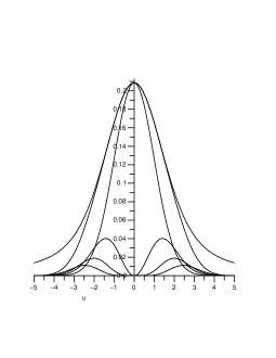
Figure 1: from top to bottom, density $f_{Z}$ in the case $d=1$, its approximation by the sum of the first four term in (3) and these first four terms

4 Proofs

4.1 Proof of Theorem 1

Using a result by Keilson and Steutel [12], a stochastic representation for the random variable $\mathbf{Z}$ is

$$\mathbf{Z}=\sigma\mathbf{N}_{1}+\frac{1}{\sqrt{2a}}\mathbf{N}_{2}\overset{d}{=}\sqrt{\sigma^{2}+\frac{1}{2a}}\mathbf{N}$$

where $\mathbf{N}$ is $d-$variate standard normal, $a$ is Gamma distributed $\Gamma\left(\nu,1\right)$ and $\overset{d}{=}$ denotes equality in distribution. The density of $\mathbf{Z}$ reads thus

$$f_{\mathbf{Z}}\left(\mathbf{z}\right)=\int_{0}^{+\infty}\frac{1}{\Gamma\left(\nu\right)}e^{-a}a^{\nu-1}\frac{1}{\left(2\pi\left(\sigma^{2}+\frac{1}{2a}\right)\right)^{\frac{d}{2}}}\exp\left(-\frac{\|\mathbf{z}\|^{2}}{2\left(\sigma^{2}+\frac{1}{2a}\right)}\right)da.$$ (14)

Since $\exp\left(-\frac{\|\mathbf{z}\|^{2}}{2\left(\sigma^{2}+\frac{1}{2a}\right)}\right)=\exp\left(-\frac{\|\mathbf{z}\|^{2}}{2\sigma^{2}}\right)\exp\left(\frac{\|\mathbf{z}\|^{2}}{2\sigma^{2}}\frac{\gamma^{2}}{a+\gamma^{2}}\right)$ with $\gamma^{2}=\frac{1}{2\sigma^{2}}$, we deduce

$$f_{\mathbf{Z}}\left(\mathbf{z}\right) = \frac{1}{\left(\sigma\sqrt{2\pi}\right)^{d}}\exp\left(-\frac{\|\mathbf{z}\|^{2}}{2\sigma^{2}}\right)\frac{1}{\Gamma\left(\nu\right)}\int_{0}^{+\infty}e^{-a}a^{\nu-1}\frac{a^{\frac{d}{2}}}{\left(a+\gamma^{2}\right)^{\frac{d}{2}}}\exp\left(\frac{\|\mathbf{z}^{2}\|}{2\sigma^{2}}\frac{\gamma^{2}}{a+\gamma^{2}}\right)da$$

$$= \frac{1}{\left(\sigma\sqrt{2\pi}\right)^{d}}\exp\left(-\frac{\|\mathbf{z}\|^{2}}{2\sigma^{2}}\right)\frac{1}{\Gamma\left(\nu\right)}\sum_{k=0}^{+\infty}\frac{\gamma^{2k}}{k!}\left(\frac{\|\mathbf{z}\|^{2}}{2\sigma^{2}}\right)^{k}\int_{0}^{+\infty}e^{-a}a^{\nu+\frac{d}{2}-1}\left(a+\gamma^{2}\right)^{-k-\frac{d}{2}}da,$$

where the interchange of the sum and the integral is justified by the Lebesgue monotone convergence theorem. Since, using [10, 4.642], $\forall k\in\mathbb{N},$

$$\int_{\mathbb{R}^{d}}\left(\frac{\|\mathbf{x}\|^{2}}{2\sigma^{2}}\right)^{k}\exp\left(-\frac{\|\mathbf{x}\|^{2}}{2\sigma^{2}}\right)d\mathbf{x}=\frac{2\pi^{\frac{d}{2}}}{\Gamma\left(\frac{d}{2}\right)}\int_{0}^{+\infty}\left(\frac{r^{2}}{2\sigma^{2}}\right)^{k}\exp\left(-\frac{r^{2}}{2\sigma^{2}}\right)r^{d-1}dr,$$

which is equal to $\frac{\pi^{\frac{d}{2}}}{\Gamma\left(\frac{d}{2}\right)}\left(\sigma\sqrt{2}\right)^{d}\Gamma\left(k+\frac{d}{2}\right),$ the function $g_{k,\sigma}$ as defined by (1) is a probability density and the result follows. Using the Kummer function

$$\Psi(\alpha,\beta;z)=\frac{1}{\Gamma(\alpha)}\int_{0}^{\infty}e^{-zt}t^{\alpha-1}(1+t)^{\beta-\alpha-1}dt,$$ (15)

cf. [10, p.1085], the integral in the expression of $f_{\mathbf{Z}}$ can be written

$$\int_{0}^{\infty}a^{\nu+\frac{d}{2}-1}e^{-a}(a+\gamma^{2})^{-k-\frac{d}{2}}da=(\gamma^{2})^{\nu-k}\Gamma(\nu+\frac{d}{2})\Psi(\nu+\frac{d}{2},\nu-k+1;\gamma^{2}).$$ (16)

4.2 Proof of Proposition 2

We have

$$\tilde{\mathbf{Z}}=a_{2}\left(\frac{a_{1}}{a_{2}}\mathbf{X}+\mathbf{T}\right)=a_{2}\left(\tilde{\sigma}\mathbf{N}_{1}+\mathbf{T}\right)=a_{2}\tilde{\mathbf{Z}}$$

with $\tilde{\sigma}=\frac{a_{1}}{a_{2}}\sigma$ so that $\tilde{\gamma}=\frac{a_{2}}{\sigma\sqrt{2}a_{1}}$ and

$$f_{\tilde{\mathbf{Z}}}\left(z\right)=\frac{1}{a_{2}^{d}}f_{\mathbf{Z}}\left(\frac{\mathbf{z}}{a_{2}}\right)=\sum_{k=0}^{+\infty}\alpha_{k}^{\left(\nu,\tilde{\gamma}\right)}\frac{1}{a_{2}^{d}}g_{k,\frac{a_{1}}{a_{2}}\sigma}\left(\frac{\mathbf{z}}{a_{2}}\right)$$

but $\frac{1}{a_{2}^{d}}g_{k,\frac{a_{1}}{a_{2}}\sigma}\left(\frac{\mathbf{z}}{a_{2}}\right)=g_{k,a_{1}\sigma}\left(\mathbf{z}\right)$ so that the result holds.

4.3 Proof of Theorem 3

Let us define $t=\frac{\sigma^{2}}{2}$ so that $\gamma=\frac{1}{\sigma\sqrt{2}}=\frac{1}{2\sqrt{t}}$ and consider the $k-$th term in the convex combination (3)

$$\alpha_{k}^{\left(\nu,\frac{1}{2\sqrt{t}}\right)}g_{k,\sqrt{2t}}\left(\mathbf{x}\right)=\frac{1}{\pi^{\frac{d}{2}}\Gamma\left(\nu\right)k!}\left(\frac{\|\mathbf{x}\|^{2}}{4t}\right)^{k}\exp\left(-\frac{\|\mathbf{x}\|^{2}}{4t}\right)\int_{0}^{+\infty}\frac{s^{\nu+\frac{d}{2}-1}\exp\left(-s\right)}{\left(1+4ts\right)^{k+\frac{d}{2}}}ds;$$

putting $w=4ts$ and subordinating with the inverse Gamma distribution yields

$$\int_{0}^{+\infty}\alpha_{k}^{\left(\nu,\frac{1}{2\sqrt{t}}\right)}g_{k,\sqrt{2t}}\left(\mathbf{x}\right)d\tilde{\gamma}_{\mu}\left(t\right) = \frac{2^{-2\mu}}{\pi^{\frac{d}{2}}\Gamma\left(\mu\right)\Gamma\left(\nu\right)}\frac{\|\mathbf{x}\|^{2k}}{k!}\int_{0}^{+\infty}\left(\frac{1}{4t}\right)^{k+\nu+\frac{d}{2}}\frac{e^{-\frac{\|\mathbf{x}\|^{2}+1}{4t}}}{t^{\mu+1}}\int_{0}^{+\infty}\frac{w^{\nu+\frac{d}{2}-1}e^{-\frac{w}{4t}}}{\left(1+w\right)^{k+\frac{d}{2}}}dwdt$$

$$= \frac{4^{-\mu-\nu-k-\frac{d}{2}}}{\pi^{\frac{d}{2}}\Gamma\left(\mu\right)\Gamma\left(\nu\right)}\frac{\|\mathbf{x}\|^{2k}}{k!}\int_{0}^{+\infty}\frac{w^{\nu+\frac{d}{2}-1}}{\left(1+w\right)^{k+\frac{d}{2}}}\int_{0}^{+\infty}\frac{e^{-\frac{w+\|\mathbf{x}\|^{2}+1}{4t}}}{t^{k+\mu+\nu+\frac{d}{2}+1}}dtdw.$$

By the change of variable $u=\frac{w+\|\mathbf{x}\|^{2}+1}{4t},$ this is equal to

$$\frac{1}{4^{\mu+\nu+k+\frac{d}{2}}\pi^{\frac{d}{2}}\Gamma\left(\mu\right)\Gamma\left(\nu\right)}\frac{\|\mathbf{x}\|^{2k}}{k!}\int_{0}^{+\infty}\frac{w^{\nu+\frac{d}{2}-1}}{\left(1+w\right)^{k+\frac{d}{2}}}\left(\frac{w+\|\mathbf{x}\|^{2}+1}{4}\right)^{-k-\mu-\nu-\frac{d}{2}}\int_{0}^{+\infty}u^{k+\mu+\nu+\frac{d}{2}-1}e^{-u}dudw$$

and, since the latter integral is a Gamma integral, to

$$\frac{\Gamma\left(\mu+\nu+k+\frac{d}{2}\right)}{\pi^{\frac{d}{2}}\Gamma\left(\mu\right)\Gamma\left(\nu\right)}\frac{\|\mathbf{x}\|^{2k}}{k!}\int_{0}^{+\infty}\frac{w^{\nu+\frac{d}{2}-1}}{\left(1+w\right)^{k+\frac{d}{2}}\left(w+\|\mathbf{x}\|^{2}+1\right)^{k+\mu+\nu+\frac{d}{2}}}dw$$

The latter integral can be identified as Euler’s integral representation of a hypergeometric function [3, Th. 2.2.1 p.65]

$$\int_{0}^{+\infty}\frac{w^{\nu+\frac{d}{2}-1}}{\left(1+w\right)^{k+\frac{d}{2}}\left(w+\|\mathbf{x}\|^{2}+1\right)^{k+\mu+\nu+\frac{d}{2}}}dw$$

$$= \frac{\Gamma\left(2k+\mu+\frac{d}{2}\right)\Gamma\left(\nu+\frac{d}{2}\right)}{\Gamma\left(2k+\mu+\nu+d\right)}{}_{2}F_{1}\left(\begin{array}[]{c}k+\mu+\nu+\frac{d}{2},\,\,2k+\mu+\frac{d}{2}\\ 2k+\mu+\nu+d\end{array};-\|\mathbf{x}\|^{2}\right)$$

so that, using Pfaff’s formula [3, 2.2.6 p.68]

$${}_{2}F_{1}\left(\begin{array}[]{c}a,\,\,b\\ c\end{array};x\right)=\left(1-x\right)^{-a}{}_{2}F_{1}\left(\begin{array}[]{c}a,\,c-b\\ c\end{array};\frac{x}{x-1}\right)$$

we deduce

$$\int_{0}^{+\infty}\alpha_{k}^{\left(\nu,\frac{1}{2\sqrt{t}}\right)}g_{k,\sqrt{2t}}\left(\mathbf{x}\right)d\tilde{\gamma}_{\mu}\left(t\right) = \frac{\Gamma\left(\mu+\nu+k+\frac{d}{2}\right)\Gamma\left(\nu+\frac{d}{2}\right)}{\pi^{\frac{d}{2}}\Gamma\left(\mu\right)\Gamma\left(\nu\right)k!}\frac{\Gamma\left(2k+\mu+\frac{d}{2}\right)}{\Gamma\left(2k+\mu+\nu+d\right)}$$

$$\times \frac{\|\mathbf{x}\|^{2k}}{\left(1+\|\mathbf{x}\|^{2}\right)^{k+\mu+\nu+\frac{d}{2}}}{}_{2}F_{1}\left(\begin{array}[]{c}k+\mu+\nu+\frac{d}{2},\,\,\nu+\frac{d}{2}\\ 2k+\mu+\nu+d\end{array};\frac{\|\mathbf{x}\|^{2}}{1+\|\mathbf{x}\|^{2}}\right).$$

Replacing the hypergeometric function by its series, we deduce

$$\int_{0}^{+\infty}\alpha_{k}^{\left(\nu,\frac{1}{2\sqrt{t}}\right)}g_{k,\sqrt{2t}}\left(\mathbf{x}\right)d\tilde{\gamma}_{\mu}\left(t\right) = \frac{\Gamma\left(\mu+\nu+k+\frac{d}{2}\right)\Gamma\left(\nu+\frac{d}{2}\right)}{\pi^{\frac{d}{2}}\Gamma\left(\mu\right)\Gamma\left(\nu\right)k!}\frac{\Gamma\left(2k+\mu+\frac{d}{2}\right)}{\Gamma\left(2k+\mu+\nu+d\right)}$$

$$\times \sum_{l=0}^{+\infty}\frac{\left(\nu+\frac{d}{2}\right)_{l}\left(k+\mu+\nu+\frac{d}{2}\right)_{l}}{\left(2k+\mu+\nu+d\right)_{l}l!}\frac{\|\mathbf{x}\|^{2k+2l}}{\left(1+\|\mathbf{x}\|^{2}\right)^{k+l+\mu+\nu+\frac{d}{2}}}$$

$$= \sum_{l=0}^{+\infty}d_{k,l}\phi_{l+k,\eta}\left(\mathbf{x}\right)$$

where $\eta=\mu+\nu,$ the density $\phi_{n,\eta}\left(\mathbf{x}\right)$ is defined by (2) and the coefficient $d_{k,l}$ is equal to

$$d_{k,l} = \frac{\Gamma\left(\mu+\nu+k+\frac{d}{2}\right)\Gamma\left(\nu+\frac{d}{2}\right)}{\pi^{\frac{d}{2}}\Gamma\left(\mu\right)\Gamma\left(\nu\right)k!}\frac{\Gamma\left(2k+\mu+\frac{d}{2}\right)}{\Gamma\left(2k+\mu+\nu+d\right)}\frac{\left(\nu+\frac{d}{2}\right)_{l}\left(k+\mu+\nu+\frac{d}{2}\right)_{l}}{\left(2k+\mu+\nu+d\right)_{l}l!}\frac{\Gamma\left(\mu+\nu\right)\Gamma\left(k+l+\frac{d}{2}\right)}{\Gamma\left(\mu+\nu+k+l+\frac{d}{2}\right)}\frac{\pi^{\frac{d}{2}}}{\Gamma\left(\frac{d}{2}\right)}$$

$$= \frac{\Gamma\left(\nu+\frac{d}{2}\right)\left(\nu+\frac{d}{2}\right)_{l}}{\Gamma\left(\mu\right)\Gamma\left(\nu\right)k!l!}\frac{\Gamma\left(2k+\mu+\frac{d}{2}\right)\Gamma\left(\mu+\nu\right)\Gamma\left(k+l+\frac{d}{2}\right)}{\Gamma\left(2k+l+\mu+\nu+d\right)\Gamma\left(\frac{d}{2}\right)}.$$

using the identity $\left(a\right)_{l}\Gamma\left(a\right)=\Gamma\left(a+l\right)$ twice. Writing $\Gamma\left(2k+\mu+\frac{d}{2}\right)=\left(\mu+\frac{d}{2}\right)_{2k}\Gamma\left(\mu+\frac{d}{2}\right),$ $\Gamma\left(k+l+\frac{d}{2}\right)=\left(\frac{d}{2}\right)_{k+l}\Gamma\left(\frac{d}{2}\right)$ and $\Gamma\left(2k+l+\mu+\nu+d\right)=\left(\mu+\nu+d\right)_{2k+l}\Gamma\left(\mu+\nu+d\right),$ we deduce

$$d_{k,l}=\frac{B\left(\nu+\frac{d}{2},\mu+\frac{d}{2}\right)}{B\left(\nu,\mu\right)k!l!}\frac{\left(\mu+\frac{d}{2}\right)_{2k}\left(\nu+\frac{d}{2}\right)_{l}\left(\frac{d}{2}\right)_{k+l}}{\left(\mu+\nu+d\right)_{2k+l}}.$$

Now the density of $\mathbf{Y}=\mathbf{T}_{1}+\mathbf{T}_{2}$ is the sum over $k$ of these terms and reads

$$f_{Y}\left(\mathbf{x}\right)=\sum_{k,l=0}^{+\infty}d_{k,l}\phi_{k+l,\eta}\left(\mathbf{x}\right).$$

We perform the change of variable $n=k+l$ to obtain

$$f_{\mathbf{Y}}\left(\mathbf{x}\right)=\sum_{n=0}^{+\infty}\phi_{n,\eta}\left(\mathbf{x}\right)\sum_{k=0}^{n}d_{k,n-k}.$$

The inner sum can be written

$$c_{n}^{\left(\nu,\mu\right)}=\sum_{k=0}^{n}d_{k,n-k} = \frac{B\left(\nu+\frac{d}{2},\mu+\frac{d}{2}\right)}{B\left(\nu,\mu\right)}\frac{\left(\frac{d}{2}\right)_{n}}{n!}\sum_{k=0}^{n}\binom{n}{k}\frac{\left(\mu+\frac{d}{2}\right)_{2k}\left(\nu+\frac{d}{2}\right)_{n-k}}{\left(\mu+\nu+d\right)_{n+k}}$$

$$=\frac{B\left(\nu+\frac{d}{2},\mu+\frac{d}{2}\right)}{B\left(\nu,\mu\right)} \frac{\left(\frac{d}{2}\right)_{n}}{\left(\mu+\nu+d\right)_{2n}n!} \sum_{k=0}^{n}\binom{n}{k}\left(\mu+\frac{d}{2}\right)_{2k}\left(\nu+\frac{d}{2}\right)_{n-k}\left(\mu+\nu+d+n+k\right)_{n-k}$$

where we have used the identity

$$\frac{1}{\left(\mu+\nu+d\right)_{n+k}}=\frac{\left(\mu+\nu+d+n+k\right)_{n-k}}{\left(\mu+\nu+d\right)_{2n}}.$$

By the Chu-Vandermonde identity [3, p.70]

$$\left(\mu+\nu+d+n+k\right)_{n-k} = \left(\left(\mu+\frac{d}{2}+2k\right)+\left(\nu+\frac{d}{2}+n-k\right)\right)_{n-k}$$

$$= \sum_{j=0}^{n-k}\binom{n-k}{j}\left(\mu+\frac{d}{2}+2k\right)_{n-k-j}\left(\nu+\frac{d}{2}+n-k\right)_{j}$$

and using the identities $\left(\mu+\frac{d}{2}\right)_{2k}\left(\mu+\frac{d}{2}+2k\right)_{n-k-j}=\left(\mu+\frac{d}{2}\right)_{n+k-j}$ and $\left(\nu+\frac{d}{2}\right)_{n-k}\left(\nu+\frac{d}{2}+n-k\right)_{j}=\left(\nu+\frac{d}{2}\right)_{n-k+j},$ we deduce

$$c_{n}^{\left(\nu,\mu\right)} = \frac{B\left(\nu+\frac{d}{2},\mu+\frac{d}{2}\right)}{B\left(\nu,\mu\right)}\frac{\left(\frac{d}{2}\right)_{n}}{\left(\mu+\nu+d\right)_{2n}n!}\sum_{k=0}^{n}\sum_{j=0}^{n-k}\binom{n}{k}\binom{n-k}{j}\left(\mu+\frac{d}{2}\right)_{n+k-j}\left(\nu+\frac{d}{2}\right)_{n-k+j}$$

$$= \frac{B\left(\nu+\frac{d}{2},\mu+\frac{d}{2}\right)}{B\left(\nu,\mu\right)}\frac{\left(\frac{d}{2}\right)_{n}}{n!}\sum_{p=-n}^{n}\binom{n}{p}_{2}\frac{\left(\mu+\frac{d}{2}\right)_{n+p}\left(\nu+\frac{d}{2}\right)_{n-p}}{\left(\mu+\nu+d\right)_{2n}},$$

where we have used the change of summation index $p=k-j$ and where the trinomial [2] coefficient $\binom{n}{p}_{2}$ is

$$\binom{n}{p}_{2}=\sum_{\underset{j+k\leq n;\,k-j=p}{j,k=0}}^{n}\binom{n}{k}\binom{n-k}{j},\,\,-n\leq p\leq n.$$

Writing $\left(\mu+\frac{d}{2}\right)_{n+p}\Gamma\left(\mu+\frac{d}{2}\right)=\Gamma\left(\mu+n+p+\frac{d}{2}\right)$ and $\left(\nu+\frac{d}{2}\right)_{n-p}\Gamma\left(\nu+\frac{d}{2}\right)=\Gamma\left(\nu+\frac{d}{2}+n-p\right)$ and replacing the resulting Beta function by its integral representation we obtain

$$c_{n}^{\left(\nu,\mu\right)}=\frac{1}{B\left(\nu,\mu\right)}\frac{\left(\frac{d}{2}\right)_{n}}{n!}\sum_{p=-n}^{n}\binom{n}{p}_{2}\int_{0}^{1}t^{\mu+n+p+\frac{d}{2}-1}\left(1-t\right)^{\nu+n-p+\frac{d}{2}-1}dt,$$

and since the generating function of the trinomial coefficient is

$$\sum_{p=-n}^{+n}\binom{n}{p}_{2}x^{p}=\left(x+x^{-1}+1\right)^{n}$$

we finally obtain

$$c_{n}^{\left(\nu,\mu\right)}=\frac{1}{B\left(\nu,\mu\right)}\frac{\left(\frac{d}{2}\right)_{n}}{n!}\int_{0}^{1}t^{\mu+n+\frac{d}{2}-1}\left(1-t\right)^{\nu+n+\frac{d}{2}-1}\left(1+\frac{t}{1-t}+\frac{1-t}{t}\right)^{n}dt$$

which is the desired result.

4.4 Proof of Theorem 6

In the case of the coefficients $\alpha_{k}^{\left(\nu,\gamma\right)},$ we can factorize

$$\alpha_{k}^{\left(\nu,\gamma\right)}=\frac{\left(\frac{d}{2}\right)_{k}}{k!}\tau_{k}$$

where

$$\tau_{k}=\frac{\left(\sigma\sqrt{2}\right)^{d}}{\Gamma\left(\nu\right)}\int_{0}^{+\infty}\frac{s^{\nu+\frac{d}{2}-1}e^{-s}}{\left(1+2\sigma^{2}s\right)^{k+\frac{d}{2}}}ds=\frac{1}{\left(2\sigma^{2}\right)^{\nu}\Gamma\left(\nu\right)}\int_{0}^{1}u^{k}\frac{\left(1-u\right)^{\nu+\frac{d}{2}-1}}{u^{\nu+1}}\exp\left(-\frac{1-u}{2\sigma^{2}u}\right)du.$$

This expression shows that the sequence $\left\{\tau_{k}\right\}$ is also a Hausdorff moment sequence (not normalized) and hence $\alpha_{k}^{\left(\nu,\gamma\right)}$ is a Hausdorff moment sequence for $d=1,2$ as product of two such sequences. It is not normalized since $\sum_{k=0}^{+\infty}\alpha_{k}^{\left(\nu,\gamma\right)}=1.$ In fact, $\frac{\left(\frac{d}{2}\right)_{k}}{k!}$ is trivially a Hausdorff moment sequence when $d=2,$ and for $d=1$ we have

$$\frac{\left(\frac{1}{2}\right)_{k}}{k!}=\frac{1}{\pi}\int_{0}^{1}\frac{s^{k}ds}{\sqrt{s\left(1-s\right)}}.$$

It is a general fact that $s_{k}=\frac{\left(a\right)_{k}}{\left(b\right)_{k}}$ is a Hausdorff moment sequence when $0<a\leq b,$ see [5, formula (26)] and if $a>b$ then $s_{k}$ is not even a Hamburger moment sequence since the Hankel determinant $D_{2}=s_{0}s_{2}-s_{1}^{2}=\frac{a\left(b-a\right)}{b^{2}\left(b+1\right)}<0.$

This shows that the density (3) is an infinite convex combination of the densities (1) and the discrete probability $\alpha^{\left(\nu,\gamma\right)}=\sum_{k=0}^{+\infty}\alpha_{k}^{\left(\nu,\gamma\right)}\delta_{k}$ is infinitely divisible for $d=1,2$ since the sequence $\left\{\alpha_{k}^{\left(\nu,\gamma\right)}\right\}$ is completely monotonic, which is the same as being a Hausdorff moment sequence.

In the case of the sequence $\left\{c_{n}^{\left(\nu,\mu\right)}\right\},$ we find

$$c_{n}^{\left(\nu,\mu\right)} = \frac{1}{B\left(\nu,\mu\right)}\frac{\left(\frac{d}{2}\right)_{n}}{n!}\int_{\frac{3}{4}}^{1}u^{n}\times$$

$$\left[\left(\frac{1}{2}-\sqrt{u-\frac{3}{4}}\right)^{\mu+\frac{d}{2}-1}\left(\frac{1}{2}+\sqrt{u-\frac{3}{4}}\right)^{\nu+\frac{d}{2}-1}+\left(\frac{1}{2}+\sqrt{u-\frac{3}{4}}\right)^{\mu+\frac{d}{2}-1}\left(\frac{1}{2}-\sqrt{u-\frac{3}{4}}\right)^{\nu+\frac{d}{2}-1}\right]\frac{du}{2\sqrt{u-\frac{3}{4}}}.$$

As before $\left\{c_{n}^{\left(\nu,\mu\right)}\right\}$ is a Hausdorff moment sequence for $d=1,2$.

4.5 Proof of Theorem 7

Although the first result can be obtained by integrating (3) over $\mathbf{z}\in\mathbb{R}^{d},$ we check it directly since the computation of the sum is instructive by itself. For any $u\in\left]-1,1\right[,$ we have by the binomial series

$$\sum_{k=0}^{+\infty}\frac{\Gamma\left(k+\frac{d}{2}\right)}{k!}u^{k}=\frac{\Gamma\left(\frac{d}{2}\right)}{\left(1-u\right)^{\frac{d}{2}}}$$ (19)

so that, with $u=\frac{\gamma^{2}}{a+\gamma^{2}}$,

$$\sum_{k=0}^{+\infty}\frac{\Gamma\left(k+\frac{d}{2}\right)}{k!}\left(\frac{\gamma^{2}}{a+\gamma^{2}}\right)^{k}=\Gamma\left(\frac{d}{2}\right)\left(\frac{a+\gamma^{2}}{a}\right)^{\frac{d}{2}}$$

and we deduce

$$\sum_{k=0}^{+\infty}\alpha_{k}^{\left(\nu,\gamma\right)} = \int_{0}^{+\infty}\frac{e^{-a}}{\Gamma\left(\nu\right)\Gamma\left(\frac{d}{2}\right)}\frac{a^{\nu+\frac{d}{2}-1}}{\left(a+\gamma^{2}\right)^{\frac{d}{2}}}\Gamma\left(\frac{d}{2}\right)\left(\frac{a+\gamma^{2}}{a}\right)^{\frac{d}{2}}da=1.$$

The expectation and variances are easily computed from the stochastic representation of $K=NB\left(\frac{d}{2},\frac{a}{1+a}\right);$ the mean of a negative binomial variable $NB\left(r,p\right)$ being $\frac{r\left(1-p\right)}{p},$

$$EK=\frac{d}{2}E\frac{\frac{1}{1+a}}{\frac{a}{1+a}}=\frac{d}{2}E\frac{1}{a}=\frac{d\gamma^{2}}{2\nu-2}$$

since $a$ is $\Gamma\left(\nu,\gamma^{2}\right).$ Since moreover, the second order moment of a negative binomial is $\frac{r\left(1-p\right)\left(1+r\left(1-p\right)\right)}{p^{2}},$ a straightforward computation gives

$$EK^{2} = \frac{d}{2}\left(E\frac{1+a}{a^{2}}+\frac{d}{2}E\frac{1}{a^{2}}\right)=\frac{d}{2}\left(1+\frac{d}{2}\right)E\frac{1}{a^{2}}+\frac{d}{2}E\frac{1}{a}$$

$$= \frac{d}{2}\left(1+\frac{d}{2}\right)\frac{\gamma^{4}}{\left(\nu-1\right)\left(\nu-2\right)}+\frac{d}{2}\frac{\gamma^{2}}{\nu-1}$$

and

$$\sigma_{K}^{2}=\frac{d}{2}\frac{\gamma^{2}}{\nu-1}\left(1+\frac{\gamma^{2}}{2}\frac{d+2\left(\nu-1\right)}{\left(\nu-1\right)\left(\nu-2\right)}\right).$$

4.6 Proof of Theorem 8

The fact that the coefficients $c_{n}^{\left(\nu,\mu\right)}$ sum to $1$ is proved in the same way as in the Proof of Theorem 7; the expectation is computed accordingly as

$$EN=\frac{d}{2}E\left(\frac{1}{t\left(1-t\right)}-1\right)$$

with

$$E\frac{1}{t\left(1-t\right)}=\frac{B\left(\nu-1,\mu-1\right)}{B\left(\nu,\mu\right)}.$$

The second order moment is similarly computed as

$$EN^{2}=\frac{d}{2}E\frac{\left(1-t\left(1-t\right)\right)\left(1+\frac{d}{2}\left(1-t\left(1-t\right)\right)\right)}{t^{2}\left(1-t\right)^{2}}=\frac{d}{2}\left(1+\frac{d}{2}\right)E\frac{1}{t^{2}\left(1-t\right)^{2}}-\frac{d\left(1+d\right)}{2}E\frac{1}{t\left(1-t\right)}+\frac{d^{2}}{4}$$

so that the variance reads

$$\sigma_{N}^{2}=\frac{d^{2}}{4}-\frac{d\left(1+d\right)}{2}\frac{B\left(\nu-1,\mu-1\right)}{B\left(\nu,\mu\right)}+\frac{d}{2}\left(1+\frac{d}{2}\right)\frac{B\left(\nu-2,\mu-2\right)}{B\left(\nu,\mu\right)}-\frac{d^{2}}{4}\left(\frac{B\left(\nu-1,\mu-1\right)}{B\left(\nu,\mu\right)}-1\right)^{2}$$

and the result follows after simplification.

4.7 Proof of Theorem 9

It is clearly enough to prove that $\lim_{\nu\to\infty}\alpha_{0}^{(\nu,\gamma)}=1$ since $0\leq\alpha_{k}^{(\nu,\gamma)}\leq 1-\alpha_{0}^{(\nu,\gamma)}$ for $k>0$. We have

$$\alpha_{0}^{(\nu,\gamma)}=\frac{1}{\Gamma(\nu)}\int_{0}^{\infty}e^{-a}a^{\nu-1}\left(1+\frac{\gamma^{2}}{a}\right)^{-d/2}\,da,$$

hence

$$1-\alpha_{0}^{(\nu,\gamma)}=\frac{1}{\Gamma(\nu)}\int_{0}^{\infty}e^{-a}a^{\nu-1}\left(1-\left(1+\frac{\gamma^{2}}{a}\right)^{-d/2}\right)\,da=\frac{d\gamma}{\Gamma(\nu)}\int_{0}^{\infty}e^{-a}a^{\nu-2}\xi\left(1+\frac{\xi^{2}}{a}\right)^{-d/2-1}\,da,$$

for some $0<\xi<\gamma$ by the mean value theorem. For $\nu>1$ we therefore get

$$1-\alpha_{0}^{(\nu,\gamma)}=\frac{d\gamma^{2}}{\Gamma(\nu)}\int_{0}^{\infty}e^{-a}a^{\nu-2}\,da=\frac{d\gamma^{2}}{\nu-1}$$

which tends to 0 for $\nu\to\infty$.

4.8 Proof of Theorem 10

The coefficients $\alpha_{k}^{(\nu,\tilde{\gamma})}$ read

$$\alpha_{k}^{(\nu,\tilde{\gamma})} = \frac{\Gamma(k+\frac{d}{2})}{k!\Gamma\left(\frac{d}{2}\right)\Gamma(\nu)}\left(\frac{\eta^{2}\left(\nu-1\right)}{\sigma^{2}}\right)^{k}\int_{0}^{+\infty}\exp(-a)a^{\nu+\frac{d}{2}-1}\left(a+\frac{\eta^{2}\left(\nu-1\right)}{\sigma^{2}}\right)^{-k-\frac{d}{2}}da$$

$$= \frac{\Gamma(k+\frac{d}{2})}{k!\Gamma\left(\frac{d}{2}\right)\Gamma(\nu)}\left(\frac{\eta^{2}}{\sigma^{2}}\right)^{k}\left(\nu-1\right)^{\nu}\int_{0}^{+\infty}\exp(-b\left(\nu-1\right))b^{\nu+\frac{d}{2}-1}\left(b+\frac{\eta^{2}}{\sigma^{2}}\right)^{-k-\frac{d}{2}}db$$

using change of variable $a=b\left(\nu-1\right).$ Let us apply Laplace’s method [16, p.278]: if $f^{\prime}\left(x_{0}\right)=0$ and $f^{\prime\prime}\left(x_{0}\right)<0$ then for large $M$,

$$\int_{a}^{b}g(x)e^{Mf(x)}dx\sim g\left(x_{0}\right)e^{Mf\left(x_{0}\right)}\sqrt{\frac{2\pi}{M|f^{\prime\prime}\left(x_{0}\right)|}}.$$

Choosing $M=\nu-1,\,f\left(x\right)=-x+\log{x},\,g(x)=x^{\frac{d}{2}}\left(x+a^{2}\right)^{-k-\frac{d}{2}}$ and $x_{0}=1$, an equivalent of the right-hand side integral reads

$$e^{-\left(\nu-1\right)}\sqrt{\frac{2\pi}{\nu-1}}\left(1+\frac{\eta^{2}}{\sigma^{2}}\right)^{-k-\frac{d}{2}}.$$

Thus an equivalent of the coefficients $\alpha_{k}^{\left(\nu,\tilde{\gamma}\right)}$ reads

$$\frac{\Gamma(k+\frac{d}{2})}{k!\Gamma\left(\frac{d}{2}\right)}\frac{\left(\nu-1\right)^{\nu-\frac{1}{2}}e^{-\left(\nu-1\right)}\sqrt{2\pi}}{\Gamma\left(\nu\right)}\left(\frac{\eta^{2}}{\sigma^{2}}\right)^{k}\left(1+\frac{\eta^{2}}{\sigma^{2}}\right)^{-k-\frac{d}{2}}$$

which, by Stirling’s formula, is equivalent to

$$\frac{\Gamma\left(k+\frac{d}{2}\right)}{k!\Gamma\left(\frac{d}{2}\right)}\left(\frac{\eta^{2}}{\sigma^{2}}\right)^{k}\left(1+\frac{\eta^{2}}{\sigma^{2}}\right)^{-k-\frac{d}{2}}.$$

As a consequence, for large values of $\nu$, the density $f_{\mathbf{Z}}$ of $\mathbf{Z}$ reads

$$f_{\mathbf{Z}}\left(\mathbf{z}\right) \sim \sum_{k=0}^{+\infty}\frac{\Gamma\left(\frac{d}{2}\right)}{\left(\sigma\sqrt{2\pi}\right)^{d}\Gamma\left(k+\frac{d}{2}\right)}\left(\frac{\|\mathbf{z}\|^{2}}{2\sigma^{2}}\right)^{k}\exp\left(-\frac{\|\mathbf{z}\|^{2}}{2\sigma^{2}}\right)\frac{\Gamma\left(k+\frac{d}{2}\right)}{k!\Gamma\left(\frac{d}{2}\right)}\left(\frac{\eta^{2}}{\sigma^{2}}\right)^{k}\left(1+\frac{\eta^{2}}{\sigma^{2}}\right)^{-k-\frac{d}{2}}$$

$$= \frac{1}{\left(\sigma\sqrt{2\pi}\right)^{d}}\frac{1}{\left(1+\frac{\eta^{2}}{\sigma^{2}}\right)^{\frac{d}{2}}}\exp\left(-\frac{\|\mathbf{z}\|^{2}}{2\sigma^{2}}\right)\exp\left(\frac{\|\mathbf{z}\|^{2}}{2\sigma^{2}}\frac{\frac{\eta^{2}}{\sigma^{2}}}{1+\frac{\eta^{2}}{\sigma^{2}}}\right)$$

$$= \frac{1}{\left(\tilde{\sigma}\sqrt{2\pi}\right)^{d}}\exp\left(-\frac{\|\mathbf{z}\|^{2}}{2\tilde{\sigma}^{2}}\right)$$

with

$$\tilde{\sigma}^{2}=\sigma^{2}+\eta^{2}.$$

4.9 Proof of Proposition 4

Conditionnally to a given value of $K=k,$ the random variable $\sigma\|\mathbf{X}_{2k+d}\|\mathbf{U}_{d}$ follows the distribution $g_{k,\sigma}$; let us check that the random variable $K$ follows a $NB\left(\frac{d}{2},\frac{a}{1+a}\right)$ compound distribution where $a$ is $\Gamma\left(\nu,\gamma^{2}\right)$: conditionnally to $a,$ such a compound distribution reads

$$p_{k}|a=\binom{k+\frac{d}{2}-1}{k}\left(\frac{a}{1+a}\right)^{\frac{d}{2}}\left(\frac{1}{1+a}\right)^{k}$$

so that

$$\alpha_{k}^{\left(\nu,\gamma\right)}=Ep_{k}|a = \binom{k+\frac{d}{2}-1}{k}\int_{0}^{+\infty}\frac{\gamma^{2\nu}}{\Gamma\left(\nu\right)}e^{-\gamma^{2}a}a^{\nu+\frac{d}{2}-1}\left(1+a\right)^{-k-\frac{d}{2}}da$$

$$= \frac{\Gamma\left(k+\frac{d}{2}\right)\gamma^{2k}}{k!\Gamma\left(\frac{d}{2}\right)\Gamma\left(\nu\right)}\int_{0}^{+\infty}e^{-b}b^{\nu+\frac{d}{2}-1}\left(\gamma^{2}+b\right)^{-k-\frac{d}{2}}db$$

by the change of variable $b=\gamma^{2}a;$ this expression coincides with (4).

4.10 Proof of Proposition 5

Conditionnally to a value of $N=n,$ the random variable $\|\mathbf{T}_{2n+d}\|\mathbf{U}_{d}$ follows the distribution $\phi_{n,\nu+\mu};$ we check that the random variable $N$ follows a $NB\left(\frac{d}{2},t\left(1-t\right)\right),$ where $t$ follows a Beta distribution with parameters $\mu$ and $\nu$: conditionnally to $t,$ this compound distribution reads

$$p_{n}|t=\binom{n+\frac{d}{2}-1}{n}t^{\frac{d}{2}}\left(1-t\right)^{\frac{d}{2}}\left(1-t\left(1-t\right)\right)^{n}$$

so that

$$c_{n}^{\left(\nu,\mu\right)} = Ep_{n}|t=\frac{1}{B\left(\nu,\mu\right)}\binom{n+\frac{d}{2}-1}{n}\int_{0}^{1}t^{\mu+\frac{d}{2}-1}\left(1-t\right)^{\nu+\frac{d}{2}-1}\left(1-t\left(1-t\right)\right)^{n}dt$$

$$= \frac{1}{B\left(\nu,\mu\right)}\frac{\Gamma\left(n+\frac{d}{2}\right)}{n!\Gamma\left(\frac{d}{2}\right)}\int_{0}^{1}t^{\mu+\frac{d}{2}-1}\left(1-t\right)^{\nu+\frac{d}{2}-1}\left(1-t\left(1-t\right)\right)^{n}dt$$

which coincides with (7).

References

• [1] M. Abramowitz, I. Stegun, Handbook of Mathematical Functions: with formulas, Graphs, and Mathematical Tables, Dover Publications, 1965.
• [2] G. Andrews, Euler’s ’exemplum memorabile inductionis fallacis’ and $q-$Trinomial Coefficients, J. Amer. Math. Soc. 3, 653–669, 1990.
• [3] G. E. Andrews, R. Askey, and R. Roy, Special Functions, Cambridge University Press, Cambridge, UK, 1st ed., Feb. 1999.
• [4] V. E. Bening, V. Yu. Korolev, On an application of the Student distribution in the theory of probability and mathematical statistics, Theory Probab. Appl., Vol. 49, No. 3 (2005), 377–391.
• [5] C. Berg, On powers of Stieltjes moment sequences, II, J. Comput. Appl. Math., Vol. 199 (2007), 23–38.
• [6] C. Berg, C. Vignat, Linearization Coefficients of Bessel Polynomials and Properties of Student t-Distributions, Constructive Approximation, Vol. 27 (2008), 15–32.
• [7] C. Berg, C. Vignat, On some results of Cufaro Petroni about Student t-processes, J. Phys. A: Math. Theor. 41 (2008) 265004.
• [8] N. Cufaro Petroni, Mixtures in nonstable Lévy processes, J. Phys. A: Math. Theor. 40 (2007), 2227–2250.
• [9] K.-T. Fang, S. Kotz, K. W. Ng, Symmetric Multivariate and Related Distributions, Monographs on Statistics and Applied Probability, Chapman & Hall/CRC, 1989.
• [10] I. S. Gradshteyn, I. M. Ryzhik, Table of Integrals, Series, and Products, Seventh Edition, Academic Press, 2007.
• [11] C. C. Heyde, N. N. Leonenko, Student Processes, Adv. Appl. Prob. 37 (2005), 342–365.
• [12] J. Keilson, F.W. Steutel, Mixtures of Distributions, Moment Inequalities and Measures of Exponentiality and Normality, Annals of Probability, Volume 2, Issue 1, Feb. 1974, 112–130.
• [13] G. P. Nason, On the sum of $t$ and Gaussian random variables, Statistics and Probability Letters 76 (2006) 1280.
• [14] H. Ruben, On the distribution of the weighted difference of two independent Student variables. J. Roy. Statist. Soc. Ser. B, 22 (1960), 188–194.
• [15] G.A. Walker, J.G. Saw, The Distribution of Linear Combinations of $t$-Variables. Journal of the American Statistical Association, Vol. 73, Issue 364, Dec. 1978, 876–878.
• [16] D.V. Widder, The Laplace Transform, Princeton University Press, 1946.
• [17] V. Witkovský, Exact distribution of positive linear combinations of inverted chi-square random variables with odd degrees of freedom. Statistics and Probability Letters 56 (2002), 45–50.