CPHT-RR0470605

CERN-PH-TH/2009-074

Open string wavefunctions
in flux compactifications
Pablo G. Cámara¹ and Fernando Marchesano²

¹Centre de Physique Théorique, UMR du CNRS 7644,
Ecole Polytechnique, 91128 Palaiseau, France

² PH-TH Division, CERN CH-1211 Geneva 23, Switzerland

Abstract

We consider compactifications of type I supergravity on manifolds with $SU(3)$ structure, in the presence of RR fluxes and magnetized D9-branes, and analyze the generalized Dirac and Laplace-Beltrami operators associated to the D9-brane worldvolume fields. These compactifications are T-dual to standard type IIB toroidal orientifolds with NSNS and RR 3-form fluxes and D3/D7 branes. By using techniques of representation theory and harmonic analysis, the spectrum of open string wavefunctions can be computed for Lie groups and their quotients, as we illustrate with explicit twisted tori examples. We find a correspondence between irreducible unitary representations of the Kaloper-Myers algebra and families of Kaluza-Klein excitations. We perform the computation of 2- and 3-point couplings for matter fields in the above flux compactifications, and compare our results with those of 4d effective supergravity.

1 Introduction

Realizing that background fluxes have a non-trivial effect on the spectrum of a string compactification has been an important step towards constructing realistic 4d string vacua. This is particularly manifest in those vacua that admit a 10d supergravity description, where compactifications with fluxes [1, 2, 3] have been shown to provide a powerful framework to address moduli stabilization and supersymmetry breaking. Indeed, in the regime of weak fluxes and constant warp factor, the effect of fluxes on the light string modes can be summarized by adding a superpotential to the 4d effective theory that arises in the fluxless limit [4]. This superpotential has then the effect of lifting a non-trivial set of moduli and producing ${\cal N}=0$ vacua at tree level [5, 6].

While the above observation has mainly been exploited for the gravity sector of the theory, it is easy to see that it also applies to the gauge sector. In particular, in the context of type II compactifications with D-branes, it has been shown that fluxes induce supersymmetric and soft term masses on the light open string degrees of freedom of the theory. This can be seen both from a microscopic [7, 8, 9] and from a 4d effective field theory viewpoint [10, 11]. In fact, in this particular case it turns out that the 4d effective sugra approach is somehow more complete that the higher dimensional results, since it allows to compute soft term masses for certain open strings modes that the analysis in terms of D-brane actions has yet not been able to deal with. These modes are nothing but open strings with twisted boundary conditions, and more precisely those arising between two stacks of intersecting and/or magnetized D-branes. Generically, these open string modes are the ones giving rise to the chiral content of the 4d effective theory [3, 12]. Hence, analyzing these modes is crucial to describe the effect of fluxes on the visible sector of a realistic string compactification.

Here we would like to improve the current situation by considering a string theory limit where the coupling between open string modes and open and closed background fluxes is well-defined. More precisely, we consider type I supergravity compactifications in the presence of gauge bundles, torsion and non-trivial RR 3-form fluxes. Due to the closed string fluxes and the torsion, the internal manifold is not Calabi-Yau, but possesses an $SU(3)$-structure. One can then analyze the effect of the closed string background fluxes on open strings by directly looking at how their presence modifies the 10d equations of motion for the fluctuations of the gauge sector of the theory. Such modification will affect the spectrum of open string modes, which in this approach are described as eigenfunctions of the flux-modified Laplace and Dirac operators. These new open string wavefunctions, together with the new couplings induced by the background fluxes, will dictate the effect of fluxes on the 4d effective action upon dimensional reduction of the 10d supergravity background.

Note that this approach of computing explicit wavefunctions and using them in the dimensional reduction is essentially the one used in [13] to compute Yukawa couplings in toroidal models with magnetized D9-branes (see also [14, 15, 16, 17]). In this sense, this work can be seen as an extension of [13] to compactifications with non-vanishing closed string fluxes. Moreover, here we will analyze the full spectrum of Kaluza-Klein modes, which in fact can also be seen as open strings with twisted boundary conditions. Finally note that, unlike in the fluxless case, the CFT techniques of [18, 19, 20, 21, 22, 23] can no longer be used and supergravity is the only available tool.

As pointed out in the literature, dimensional reduction in a fluxed closed string background presents several subtleties that need to be addressed. In fact, a concrete prescription for performing a consistent 4d truncation of the theory in twisted tori (and more generical, in manifolds with SU(3) structure) is missing. The common practice is then to use instead the harmonic expansion of a standard torsionless manifold. This indeed produces the right results for the light modes in the 4d supergravity regime. Here we will follow an alternative, more controlled strategy and use techniques of non-commutative harmonic analysis to explicitly solve for the spectrum of eigenmodes of the flux-modified Dirac and Laplace operators. In this way, we perform the computation of wavefunctions for massless and massive Kaluza-Klein modes of vector bosons, scalars, fermions and matter fields for magnetized D-branes in simple type I flux compactifications. Interestingly, we find that the resulting spectrum can be classified in terms of irreducible unitary representations of the Kaloper-Myers gauge algebra [27].

The computation of the above wavefunctions carries a lot of information, that can be used for several phenomenological applications. First, by means of this formalism we can show explicitly that some wavefunctions in flux compactifications are insensitive to the flux background. Thus, if those are the lightest modes of the spectrum (as is indeed the case for weak fluxes), it is justified to expand the fluctuations in fluxless harmonics. We can also compute physical observables in the 4d effective theory, such as Yukawa couplings, in terms of overlap integrals of the corresponding wavefunctions. As a last application, one may consider integrating the spectrum of massive charged excitations in order to compute threshold corrections to the physical gauge couplings. This will however be addressed in a separate publication [28].

The above techniques are applied to three different classes of vacua: $\mathcal{N}=2$ vacua without flux-induced masses in the open string sector, $\mathcal{N}=1$ vacua with flux-induced $\mu$-terms and $\mathcal{N}=0$ vacua, and more precisely to explicit examples based on twisted tori. These examples are T-dual to type IIB flux compactifications with D3/D7-branes [5, 6] and S-dual to heterotic compactifications with torsion [29, 30]. It is then easy to see that our analysis can be easily extended to other families of flux compactifications.

The outline of the paper is as follows. In Section 2 we identify the class of type I flux vacua that we consider in the paper, and compute the modified Dirac and Laplace operators for their open string modes. We also provide two explicit supersymmetric examples of such vacua, to which we will apply our techniques in the sections to follow. Indeed, in Section 3 we address the computation of the wavefunctions for gauge bosons and introduce the necessary tools to solve for the spectrum of the Laplace-Beltrami operator in arbitrary twisted tori. Sections 4 and 5 are devoted respectively to the computation of wavefunctions for neutral scalars and fermions and, finally, matter field wavefunctions are considered in Section 6. In Section 7 we summarize the structure of massive excitations previously obtained, and then compare our results to those obtained from a 4d supergravity approach. We also translate our results to the more familiar context of type IIB flux compactifications. Section 8 contains our conclusions, while the most technical material has been left for the appendices. In particular, in Appendix C we show that our approach can also be applied to ${\cal N}=0$ vacua.

2 Dirac and Laplace equations in type I flux vacua

2.1 Type I Dirac and Laplace equations

A simple way to construct a theory of gravity and non-Abelian gauge interactions is to consider the low-energy limit of either heterotic or type I superstring theories. Indeed, in such limit we obtain a 10d ${\cal N}=1$ supergravity whose bosonic and fermionic degrees of freedom are contained in a gravity and a vector multiplet as

$$\begin{array}[]{ccc}&\text{bosons}&\text{fermions}\\ \text{\bf gravity}&g_{MN},C_{MN},\phi&\psi_{M},\lambda\\ \text{\bf vector}&A_{M}^{\alpha}&\chi^{\alpha}\end{array}$$

The gravitational content is then given by the 10d metric $g$, the two-form $C_{2}$, the dilaton $\phi$ and the Majorana-Weyl fermions $\psi$ and $\lambda$, respectively dubbed gravitino and dilatino. The vector multiplet is that of 10d ${\cal N}=1$ Yang-Mills theory, with both the gauge vector $A$ and the gaugino $\chi$ transforming in the adjoint of the gauge group $G_{gauge}$.

Both multiplets couple to each other via a relatively simple 10d ${\cal N}=1$ action which, in the Einstein frame, is given by [31, 32, 33]

$$S=-\int dx^{10}(\textrm{det }g)^{1/2}\textrm{Tr}\left[\frac{e^{\phi/2}}{4}F^{\alpha}_{MN}F^{\alpha,MN}+\bar{\chi}^{\alpha}\Gamma^{M}D_{M}\chi^{\alpha}+\frac{e^{\phi}}{24}F_{MNP}F^{MNP}\right.\\ \left.+\frac{1}{24}e^{\phi/2}F_{MNP}\bar{\chi}^{\alpha}\Gamma^{MNP}\chi^{\alpha}-\frac{1}{2}e^{\phi/4}F_{MN}^{\alpha}\bar{\chi}^{\alpha}\Gamma^{Q}\Gamma^{MN}(\psi_{Q}+\frac{\sqrt{2}}{12}\Gamma_{Q}\lambda)+\dots\right]$$ (2.1)

where all terms not involving $A$ or $\chi$ have been dropped. Here $F_{MN}$ and $F_{MNP}$ are gauge-invariant field strengths

$$F^{\alpha}_{MN}\,=\,\partial_{M}A_{N}^{\alpha}-\partial_{N}A_{M}^{\alpha}+g^{\alpha}_{\beta\gamma}A^{\beta}_{M}A^{\gamma}_{N}$$ (2.2)

$$F_{MNP}\,=\,3!\partial_{[M}C_{NP]}+3!\ A^{\alpha}_{[M}\partial_{N}A_{P]}^{\alpha}+2g_{\alpha\beta\gamma}A^{\alpha}_{M}A^{\beta}_{N}A^{\gamma}_{P}$$ (2.3)

that will be respectively written as $F_{2}$ and $F_{3}$ when expressed in $p$-form language. Finally the gauge-covariant derivative $D_{M}$ acts on the gaugino as

$$D_{M}\chi^{\alpha}\,=\,\nabla_{M}\chi^{\alpha}+g^{\alpha}_{\beta\gamma}A^{\beta}_{M}\chi^{\gamma}$$ (2.4)

with $g^{\alpha}_{\beta\gamma}$ the structure constant of $G_{gauge}$.

In bosonic backgrounds $\langle\psi\rangle=\langle\lambda\rangle\equiv 0$, and so the last piece of (2.1) does not contribute to the equations of motion for the components of the vector multiplet. Applying the Euler-Lagrange equations, it is easy to see that those read

$$\left(\not{D}+\frac{1}{4}e^{\phi/2}\not{F}_{3}\right)\chi\,=\,0$$ (2.5)

$$\nabla_{K}F^{KP}-i[A_{K},F^{KP}]-\frac{e^{\phi/2}}{2}F_{MN}F^{MNP}=0$$ (2.6)

where we have introduced the slashed notation $\not{A}_{n}\equiv\frac{1}{n!}A_{i_{1}\ldots i_{n}}\Gamma^{i_{1}\ldots i_{n}}$, and we have made use of the equation of motion for $F_{3}$ to discard terms proportional to $\nabla_{n}F^{nkp}$ in (2.6).

In the spirit of [29], let us consider 4d vacua with non-trivial $F_{3}$. In order to preserve 4d Poincaré invariance one imposes an Einstein frame ansatz of the form

$$ds^{2}\,=\,Z^{-1/2}ds^{2}_{\mathbb{R}^{1,3}}+ds^{2}_{{\cal M}_{6}}$$ (2.7)

where the warp factor $Z$ only depends on ${\cal M}_{6}$, as well as all $F_{3}$ indices lie along ${\cal M}_{6}$. In general, vacua of this kind are such that ${\cal M}_{6}$ admits an SU(3) structure, specified in terms of two globally well-defined SU(3) invariant forms $J$ and $\Omega$. In particular, we consider backgrounds where the following relations are satisfied

$$Ze^{\phi} \equiv g_{s}\,=\,\text{const.}$$ (2.8)

$$g_{s}^{1/2}e^{\phi/2}F_{3} = *_{{\cal M}_{6}}\,e^{-3\phi/2}d(e^{3\phi/2}J)$$ (2.9)

$$d\left(e^{\phi}J\wedge J\right) = 0$$ (2.10)

Note that these equations are less restrictive than those obtained in [29]. As discussed in [34, 11, 35], these are necessary conditions to construct a 4d vacuum of no-scale type. Sufficiency conditions also involve a constraint on $d\Omega$, which for supersymmetric vacua reads $d(Z^{-5/4}\Omega)=0$ and implies that ${\cal M}_{6}$ is a complex manifold.

Due to the presence of $F_{3}$, the compactification manifold ${\cal M}_{6}$ has intrinsic torsion and it is not Calabi-Yau. As a result, the usual Dirac and Laplace equations of Calabi-Yau compactifications are also modified. Let us then compute the new equations via a general dimensional reduction of eqs.(2.5) and (2.6) to 4d, closely following [13]. For simplicity, we will consider a $U(N)$ gauge field $A$. It can then be expanded as

$$A_{M}=B_{M}^{\alpha}U_{\alpha}+W^{\alpha\beta}_{M}e_{\alpha\beta}$$ (2.11)

with $B^{\alpha}_{M}$ real and $(W^{\alpha\beta}_{M})^{*}=W^{\beta\alpha}_{M}$. The $U(N)$ generators $U_{\alpha}$ and $e_{\alpha\beta}$ are given by

$$(U_{\alpha})_{ij}=\delta_{\alpha i}\delta_{\alpha j}\quad\quad(e_{\alpha\beta})_{ij}=\delta_{\alpha i}\delta_{\beta j}\quad\quad\alpha\neq\beta$$ (2.12)

In general, when performing a dimensional reduction on an SU(3)-structure manifold several subtleties arise. The first and most important one concerns the identification of a suitable basis to expand the four dimensional fluctuations [24], since different choices should be related by highly non-trivial field redefinitions in the 4d effective theory. In our computations below, we find convenient to expand the vector fields in terms of vielbein 1-forms $e^{m}$ of ${\cal M}_{6}$

$$B(x^{\mu},x^{i}) \ =\ b_{\mu}(x^{\mu})\ B(x^{i})\ dx^{\mu}\ +\ \sum_{m}b^{m}(x^{\mu})\ [\langle B^{m}\rangle+\xi^{m}](x^{i})\ e^{m}$$ (2.13)

$$W(x^{\mu},x^{i}) \ =\ w_{\mu}(x^{\mu})\ W(x^{i})\ dx^{\mu}\ +\ \sum_{m}w^{m}(x^{\mu})\ \Phi^{m}(x^{i})\ e^{m}$$ (2.14)

where $x^{\mu}$, $x^{i}$ denote respectively the 4d Minkowski and 6d internal coordinates. Here, as in [13], we have set $\langle W\rangle=0$ and allowed for a non-trivial internal vev for $B$, which breaks the initial $U(N)$ gauge group into a subgroup $G_{unbr}=\prod_{i}U(n_{i})\subset U(N)$. The modes $b_{\mu}(x^{\mu})$, $w_{\mu}(x^{\mu})$, and $b^{m}(x^{\mu})$, $w^{m}(x^{\mu})$ transform respectively as 4d Lorentz vector and scalar fields, while from the point of view of $G_{unbr}$ the $b$’s transform in the adjoint and the $w$’s in the bifundamental representation. Finally, these modes satisfy standard equations of motion for 4d gauge bosons

$$\nabla_{\mu}F^{\mu\nu}-i[A_{\mu},F^{\mu\nu}]=m^{2}_{A}A^{\nu}$$ (2.15)

and Klein-Gordon fields

$$\nabla^{2}_{\mathbb{R}^{1,3}}b^{m} =m^{2}_{\xi}\ b^{m}$$ (2.16)

$$\nabla^{2}_{\mathbb{R}^{1,3}}w^{m} =m^{2}_{\Phi}\ w^{m}$$ (2.17)

where in (2.15) $A_{\mu}=b_{\mu}+w_{\mu}$ and $m^{2}_{A}=m^{2}_{B}+m^{2}_{W}$.

Similarly, the 10d Majorana-Weyl spinor $\chi$ can be decomposed as

$$\chi\,=\,\zeta+\mathcal{B}^{*}\zeta^{*}\quad\quad\zeta\,=\,\chi_{4}\otimes\chi_{6}$$ (2.18)

where $\chi_{6}$ is a 6d Weyl spinor of negative chirality, $\mathcal{B}=\mathcal{B}_{4}\otimes\mathcal{B}_{6}$ a Majorana matrix and $\chi_{4}$ is a 4d Weyl spinor of positive chirality satisfying

$$\gamma_{(4)}\not{\partial}_{\mathbb{R}^{1,3}}\mathcal{B}_{4}^{*}\chi_{4}^{*}=-m_{\chi}\,\chi_{4}$$ (2.19)

where the 4d fermionic modes will arise from. Just as in eqs.(2.13), (2.14), in the decomposition (2.18) there is a choice of basis for the 4d fluctuation modes, now implicit in the definition of $\chi_{6}$. Such choice of basis is given in Appendix A, where the fermion conventions used in this paper are specified. As one can check explicitly in the examples below, the choices performed in the bosonic and fermionic sectors are related to each other via the 10d supersymmetry variation

$$\delta_{\epsilon}A_{M}\,=\,\frac{i}{2}\bar{\epsilon}\,\Gamma_{M}\chi$$ (2.20)

where $\epsilon$ is the 10d Killing spinor of the background. As a result, the effective theory obtained from the above dimensional reduction scheme will inherit a 4d SUSY structure that can be obtained directly from reducing (2.20).

In general, in order to fully specify the 4d couplings of the effective action one first needs to compute internal wavefunctions of the fields $B(y)$, $W(y)$, $\xi^{m}(y)$, $\Phi^{m}(y)$ and $\chi_{6}(y)$ that appear in eqs.(2.13), (2.14) and (2.18). Such wavefunctions can be obtained by solving the corresponding internal 6d Dirac and Laplace equations for a type I background with fluxes. One can compute these equations by plugging (2.13)-(2.19) into (2.5)-(2.6) and the ansatz (2.7). We obtain

$$\nabla^{\mathcal{M}_{6}}{}^{m}\nabla^{\mathcal{M}_{6}}_{m}B-(\partial_{m}\textrm{log }Z)\nabla^{\mathcal{M}_{6}}{}^{m}B\,=\,-Z^{1/2}m_{B}^{2}B$$ (2.21)

$$\tilde{D}^{m}\tilde{D}_{m}W-2(\partial_{m}\textrm{log}Z)\tilde{D}^{m}W\,=\,-Z^{1/2}m_{W}^{2}W$$ (2.22)

$$\nabla^{\mathcal{M}_{6}}{}^{m}\nabla^{\mathcal{M}_{6}}_{m}\xi^{p,\alpha}-[\nabla_{m}^{\mathcal{M}_{6}},\nabla^{\mathcal{M}_{6}}{}^{p}]\xi^{m,\alpha}-2(\partial_{k}\textrm{log }Z)\nabla^{\mathcal{M}_{6}}{}^{[k}\xi^{p],\alpha}+\\ +e^{\phi/2}(\nabla^{\mathcal{M}_{6}}_{m}\xi^{n,\alpha})F_{n}{}^{mp}=-Z^{1/2}m_{\xi}^{2}\xi^{p,\alpha}$$ (2.23)

$$\tilde{D}^{m}\tilde{D}_{m}\Phi^{p,\alpha\beta}-[\nabla_{m}^{\mathcal{M}_{6}},\nabla^{\mathcal{M}_{6}}{}^{p}]\Phi^{m,\alpha\beta}-2(\partial_{k}\textrm{log }Z)\tilde{D}^{[k}\Phi^{p],\alpha\beta}+2i\Phi^{m,\alpha\beta}\langle G_{m}{}^{p,\alpha\beta}\rangle+\\ +e^{\phi/2}(\tilde{D}_{m}\Phi^{n,\alpha\beta})F_{n}{}^{mp}=-Z^{1/2}m_{\Phi}^{2}\Phi^{p,\alpha\beta}$$ (2.24)

for the bosonic wavefunctions and

$$\Gamma_{(4)}\left(\not{D}^{{\cal M}_{6}}+\frac{1}{4}e^{\phi/2}\not{F}_{3}-\frac{1}{2}\not{\partial}\ln Z\right)\chi_{6}\,=\,Z^{1/4}m_{\chi}\,\mathcal{B}_{6}^{*}\chi_{6}^{*}$$ (2.25)

for the fermionic wavefunctions, where $\nabla^{\mathcal{M}_{6}}_{m}$ and $\not{D}^{{\cal M}_{6}}=\Gamma^{m}D_{m}$ are the bosonic and fermionic covariant derivatives in ${\cal M}_{6}$ and we have introduced the notation

$$\tilde{D}_{m}\Phi^{\alpha\beta}_{n}=\nabla_{m}^{\mathcal{M}_{6}}\Phi^{\alpha\beta}_{n}-i(\langle B^{\alpha}_{m}\rangle-\langle B^{\beta}_{m}\rangle)\Phi^{\alpha\beta}_{n}$$ (2.26)

$$\langle G^{\alpha\beta}_{mn}\rangle=2\nabla_{[m}^{\mathcal{M}_{6}}\langle B^{\alpha}_{n]}\rangle-2\nabla_{[m}^{\mathcal{M}_{6}}\langle B^{\beta}_{n]}\rangle$$ (2.27)

Finally, note that if we expand the fermionic wavefunction as $\chi_{6}=\lambda^{\alpha}U_{\alpha}+\Psi^{\alpha\beta}e_{\alpha\beta}$, we have that $\not{D}^{{\cal M}_{6}}\lambda^{\alpha}=\not{\nabla}^{{\cal M}_{6}}\lambda^{\alpha}$ and $\not{D}^{{\cal M}_{6}}\Psi^{\alpha\beta}=\tilde{\not{D}}\Psi^{\alpha\beta}$.

2.2 Elliptic fibrations

A simple way to find solutions to the equations (2.8)-(2.10) is to consider the particular case where ${\cal M}_{6}$ is an elliptic fibration of fiber $\Pi_{2}$ over a four dimensional base $B_{4}$ [5, 34, 11, 35]. In particular, we consider a metric ansatz of the form

$$ds^{2}_{{\cal M}_{6}}\,=\,Z^{-1/2}\sum_{a\in\Pi_{2}}\left(e^{a}\right)^{2}+Z^{3/2}ds^{2}_{B_{4}}$$ (2.28)

where neither the base metric $ds^{2}_{B_{4}}$ nor the vielbein 1-forms of the fiber $e^{a}$ depend on the warp factor $Z$, which in turn only depends on the $B_{4}$ coordinates. This will be indeed the case if $Z$ is sourced by background fluxes and/or D5-branes/O5-planes wrapped on $\Pi_{2}$ (see e.g. [34, 35] for explicit examples of this kind). The structure of the (unwarped) fibration can then be parameterized as

$$de^{a}=\frac{1}{2}f^{a}_{mn}e^{m}\wedge e^{n}\in H^{2}(B_{4},\mathbb{R})$$ (2.29)

with $f^{a}_{mn}$ some structure constants.

In general, $\nabla^{\mathcal{M}_{6}}_{m}$, $\not{D}^{{\cal M}_{6}}$ and $e^{\phi/2}\not{F}$ will depend on the warp factor $Z$, that will enter eqs.(2.21)-(2.25) in a rather non-trivial way. Even if as shown in Appendix B the on-shell relations (2.8)-(2.10) simplify such dependence, we would like to simplify the problem by taking a limit of constant warp factor. In practice, one can achieve such limit via the non-isotropic fibration $\textrm{Vol}_{B_{4}}^{1/2}\gg\textrm{Vol}_{\Pi_{2}}$, that in terms of mass scales translates into the hierarchy $m^{\text{KK}}_{\text{fib}}\gg m^{\text{KK}}_{\text{base}}\gg m_{\text{flux}}$ [34]. Here $m_{\text{flux}}$ (denoted $\varepsilon$ in the following sections) is the mass scale introduced by the presence of background fluxes, and in particular the mass scale of closed and open string lifted moduli. As a result, this hierarchy of scales is essential to understand the process of moduli stabilization in terms of a 4d ${\cal N}=1$ effective theory where all KK modes have been integrated out. In addition, as discussed in section 7.2 the condition $m^{\text{KK}}_{\text{base}}\gg m_{\text{flux}}$ also ensures that the warp factor can be taken to be constant, which is the approximation that we would like to consider in the following. Finally, imposing $\textrm{Vol}_{B_{4}}^{1/2},\textrm{Vol}_{\Pi_{2}}\gg\alpha^{\prime}$ guarantees that the supergravity approximation in which we are working remains valid.

Splitting the 2-form $J$ as $J=J_{\Pi_{2}}+J_{B_{4}}$ as in [11], introducing the projectors,

$$P_{\pm}^{\Pi_{2}}\,=\,\frac{1}{2}\left(1\pm i\not{J}_{\Pi_{2}}\gamma_{(6)}\right)$$ (2.30)

and taking $Z$ constant eq.(2.25) becomes (see Appendix B)

$$\left(\not{D}^{\Pi_{2}}+\not{D}^{B_{4}}+\frac{1}{2}\not{f}P_{+}^{\Pi_{2}}\right)\chi_{6}\,=\,m_{\chi}\,\mathcal{B}_{6}^{*}\chi_{6}^{*}$$ (2.31)

where we have absorbed the operator $\Gamma_{(4)}$ in the definition of slashed contraction. Indeed, in the expression above all slashed quantities are constructed from the set of $\Gamma$-matrices defined in (A.9), a convention that we will take from now on. Finally, we have defined the antisymmetrized geometric flux

$$f_{mnp}\,=\,3\,\delta_{r[m}f^{r}_{np]}$$ (2.32)

The projector $P_{+}^{\Pi_{2}}$ corresponds to the chirality projector of the 4d base $B_{4}$. One can then split the internal 6d fermion as

$$\chi_{6}\,=\,\chi_{\Pi_{2}}+\chi_{B_{4}}$$ (2.33)

where $\chi_{\Pi_{2},B_{4}}$ satisfy $P_{+}^{\Pi_{2}}\chi_{\Pi_{2}}=\chi_{\Pi_{2}}$ and $P_{+}^{\Pi_{2}}\chi_{B_{4}}=0$. Since $\mathcal{B}_{6}$ changes the fiber chirality but not the base chirality, we can split the Dirac equation as

$${\not{D}}^{\Pi_{2}}\chi_{B_{4}}+{\not{D}}^{B_{4}}\chi_{\Pi_{2}} = m_{\chi}\mathcal{B}_{6}^{*}\chi_{B_{4}}^{*}$$ (2.34)

$${\not{D}}^{\Pi_{2}}\chi_{\Pi_{2}}+{\not{D}}^{B_{4}}\chi_{B_{4}}+\frac{1}{2}{\not{f}}\chi_{\Pi_{2}} = m_{\chi}\mathcal{B}_{6}^{*}\chi_{\Pi_{2}}^{*}$$ (2.35)

A similar analysis can be carried out for the scalar wavefunctions, governed by eqs.(2.23) and (2.24). Distinguishing between scalars corresponding to the base and to the fiber, the equations of motion (2.23) and (2.24) read

$$\hat{\partial}_{m}\hat{\partial}^{m}\xi^{p}_{\Pi_{2}}-(f^{p}_{mn}-e^{\phi/2}F_{nm}{}^{p})\hat{\partial}^{m}\xi^{n}_{B_{4}}-\frac{1}{2}f^{a}_{mn}(f^{p}_{mn}-e^{\phi/2}F_{nm}{}^{p})\xi^{a}_{\Pi_{2}}=-m_{\xi}^{2}\xi^{p}_{\Pi_{2}}$$ (2.36)

$$\hat{\partial}_{m}\hat{\partial}^{m}\xi^{p}_{B_{4}}-(f^{m}_{pn}-e^{\phi/2}F_{n{m}}{}^{p})\hat{\partial}^{m}\xi^{n}_{B_{4}}+(f_{mp}^{n}+e^{\phi/2}F_{{n}m}{}^{p})\hat{\partial}^{m}\xi^{n}_{\Pi_{2}}=-m_{\xi}^{2}\xi_{B_{4}}^{p}$$ (2.37)

and

$$\hat{D}_{m}\hat{D}^{m}\Phi^{p}_{\Pi_{2}}-(f^{p}_{mn}-e^{\phi/2}F_{nm}{}^{p})\hat{D}^{m}\Phi^{n}_{B_{4}}-\frac{1}{2}f^{a}_{mn}(f^{p}_{mn}-e^{\phi/2}F_{nm}{}^{p})\Phi^{a}_{\Pi_{2}}=-m_{\Phi}^{2}\Phi^{p}_{\Pi_{2}}$$ (2.38)

$$\hat{D}_{m}\hat{D}^{m}\Phi^{p}_{B_{4}}-(f^{m}_{pn}-e^{\phi/2}F_{n{m}}{}^{p})\hat{D}^{m}\Phi^{n}_{B_{4}}+(f_{mp}^{n}+e^{\phi/2}F_{{n}m}{}^{p})\hat{D}^{m}\Phi^{n}_{\Pi_{2}}+2i\Phi_{\Pi_{2}}^{m}\langle\hat{G}_{m}{}^{p}\rangle$$

$$\hskip 312.9803pt=-m_{\Phi}^{2}\Phi_{B_{4}}^{p}$$ (2.39)

where $\hat{D}_{m}\Phi_{n}^{\alpha\beta}$ and $\langle\hat{G}^{\alpha\beta}_{mn}\rangle$ are respectively defined as in (2.26) and (2.27), but replacing the covariant derivative $\nabla_{m}^{\mathcal{M}_{6}}$ by twisted derivatives defined in terms of the vielbein as

$$\hat{\partial}_{a}\equiv e_{a}{}^{\alpha}(x)\ \partial_{x^{\alpha}}$$ (2.40)

Finally, we have assumed that $\langle B_{m}^{\alpha}\rangle$ is constant along the fiber, as dictated by cancelation of Freed-Witten anomalies [41, 27].

2.3 Twisted tori examples

In order to provide explicit examples of the metric ansatz (2.28) one may consider the simple case where the base of the fibration $B_{4}$ corresponds to a flat four-torus $T^{4}$. This basically implies that, up to warp factors, ${\cal M}_{6}$ lies within a particular class of twisted tori, which are in fact the simplest non-trivial examples of SU(3) structure manifold. A very interesting feature of twisted tori, and which will be crucial in the discussion of next section, is that they can be defined in a group theoretic way, and more precisely as a left quotient of groups ${\cal M}_{6}=\Gamma\backslash G$.

Indeed, let us consider a $d$-dimensional group manifold $G$ and its Lie algebra $\mathfrak{g}=\textrm{Lie}(G)$. The latter is specified by a set of structure constants $f^{a}_{bc}$ that satisfy the Jacobi identity $f^{a}_{[bc}f^{g}_{d]a}=0$. In terms of a matrix representation of the Lie Group $g_{G}\in GL(n)$, one can easily compute the vielbein left-invariant 1-forms as $g_{G}^{-1}dg_{G}=e^{a}\mathfrak{t}_{a}$, with $\mathfrak{t}_{a}\in\mathfrak{g}$ the algebra generators, and hence the structure constants via

$$de^{a}=\frac{1}{2}f^{a}_{bc}e^{b}\wedge e^{c}\quad\quad\Leftrightarrow\quad\quad[\hat{\partial}_{b},\hat{\partial}_{c}]=-f^{a}_{bc}\hat{\partial}_{a}$$ (2.41)

with $\hat{\partial}_{a}$ defined as in (2.40). These twisted derivatives can then be identified with $\mathfrak{t}_{a}$. While in general $G$ may not be a compact manifold, one can construct such manifold by left-quotienting $G$ by a discrete, cocompact subgroup $\Gamma\subset G$. The resulting twisted torus ${\cal M}_{d}=\Gamma\backslash G$ is no longer a group, but it is a parallelizable manifold since the left-invariant 1-forms are still globally well-defined.

Given a set of structure constants $f^{a}_{bc}$, constructing a compact manifold ${\cal M}_{d}=\Gamma\backslash G$ is usually a non-trivial problem. This is however greatly simplified if we restrict ourselves to the case where $\mathfrak{g}$ is a nilpotent Lie algebra. That is, we consider the case where the series $\{\mathfrak{g}_{s}\equiv[\mathfrak{g}_{s-1},\mathfrak{g}_{0}]\}$, with $\mathfrak{g}_{0}\equiv\mathfrak{g}=\textrm{Lie}(G)$, has $k$ non-vanishing elements, in which case $\mathfrak{g}$ is said to be $k$-step nilpotent. Then, in order for a cocompact $\Gamma$ to exist, we only need to require that $f^{a}_{ab}=0$ and that the structure constants are integers in some particular basis [46]. The resulting nilmanifold is a non-flat, compact (usually iterated) fibration of tori. In particular, we will obtain elliptic fibrations that fit into our metric ansatz (2.28).

If in particular we consider an elliptic fibration over $T^{d-2}$, then $\mathfrak{g}$ should be 2-step nilpotent. The associated Lie group has then the following faithful representation

$$g_{G}=\begin{pmatrix}{\mathbb{I}}_{d}-\frac{1}{2}ad_{\vec{X}}&\vec{X}\\ 0&1\end{pmatrix}\quad\quad\quad[ad_{\vec{X}}]^{i}_{j}\,=\,X^{k}f^{i}_{kj}$$ (2.42)

in terms of $GL(d+1,\mathbb{R})$ matrices. Here $\vec{X}$ is a $d$-dimensional coordinate vector parameterizing $\mathfrak{g}$ and $ad$ is the adjoint representation of the algebra, which due to 2-step nilpotency satisfies $ad^{2}=0$. Note that this implies that $e^{i}=dX^{i}+\frac{1}{2}f^{i}_{kj}X^{k}dX^{j}$.

A classical example of this construction is given by the $(2p+1)$-dimensional Heisenberg manifold $\mathcal{H}_{2p+1}$, the canonical example of nilpotent Lie group. Here we can split $\vec{X}^{t}=(z,\vec{x}^{\,t},\vec{y}^{\,t})$, $\vec{x},\vec{y}\in\mathbb{R}^{p}$ and express the algebra as

$$[\mathfrak{t}_{x^{i}},\mathfrak{t}_{y^{j}}]\,=\,\delta_{ij}\,\mathfrak{t}_{z}$$ (2.43)

so that (2.42) reads

$$g_{\mathcal{H}_{2p+1}}\,=\,\begin{pmatrix}1&-\frac{1}{2}\vec{y}^{\,t}&\frac{1}{2}\vec{x}^{\,t}&z\\ 0&1&0&\vec{x}\\ 0&0&1&\vec{y}\\ 0&0&0&1\end{pmatrix}$$ (2.44)

In this case, a suitable choice for $\Gamma$ is the lattice $\Gamma_{{\cal H}_{2p+1}}=\{(\vec{x},\vec{y},z)=M(\vec{n}_{x},\vec{n}_{y},n_{z})\}$ with $M,n_{z}\in\mathbb{Z}$ and $\vec{n}_{x},\vec{n}_{y}\in\mathbb{Z}^{n}$. One can then normalize the generators as $\tilde{\mathfrak{t}}_{a}=M\mathfrak{t}_{a}$, so that the algebra becomes $[\tilde{\mathfrak{t}}_{x^{i}},\tilde{\mathfrak{t}}_{y^{j}}]\,=\,\delta_{ij}M\,\tilde{\mathfrak{t}}_{z}$ and the invariant 1-forms read

$$\tilde{e}^{z}\,=\,dz-\frac{M}{2}\left(\vec{x}^{\,t}d\vec{y}-\vec{y}^{\,t}d\vec{x}\right)\quad\quad\tilde{e}^{x^{i}}\,=\,dx^{i}\quad\quad\tilde{e}^{y^{i}}\,=\,dy^{i}$$ (2.45)

The nilmanifold $\Gamma\backslash G$ then corresponds to an $S^{1}$ fibration (whose fiber is parameterized by $z$) over a $T^{2p}$ (parameterized by $(\vec{x},\vec{y})$) and of Chern class $F_{2}=M\sum_{i}dy^{i}\wedge dx^{i}$. Such U(1)-bundle structure will become manifest below, when analyzing the spectrum of the Laplace and Dirac operators in the (compactified) Heisenberg manifold. Finally, a rescaling of the form $\tilde{\mathfrak{t}}_{a}\rightarrow(2\pi R_{a})^{-1}\tilde{\mathfrak{t}}_{a}$, $X^{a}\rightarrow 2\pi R_{a}\,X^{a}$ will take us to a moduli-dependent set of structure constants, which are those that correspond to the set of vielbein left-invariant 1-forms in (2.29) and (2.41).

It follows from the above discussion that a good starting point to construct explicit solutions to eqs.(2.8)-(2.10) is to consider ${\cal M}_{6}$ to be either a nilmanifold or a product like $S^{1}\times\Gamma_{{\cal H}_{5}}\backslash{\cal H}_{5}$. In the following we will provide two different type I backgrounds based on such strategy, for which we will later on explicitly solve the Laplace and Dirac equations (see Sections 3 to 6).

According to the open string spectrum, we can roughly classify nilmanifold type I flux vacua in two different classes. The first one is that where the spectrum of massless open string adjoint scalars $b^{m}$ (see (2.13)) remains identical with respect to a toroidal (or toroidal orientifold), fluxless compactification. The second class is that where, because of the presence of the flux, some of these adjoint scalars develop up a mass of the order of $m_{\text{flux}}$, just like the closed string moduli of the compactification. We will dub such classes of vacua as vacua with vanishing and non-vanishing flux-generated $\mu$-term, respectively, and present a supersymmetric example for each of them below. A non-supersymmetric type I flux vacua will be considered in Appendix C.

2.3.1 Example with vanishing $\mu$-terms

Let us consider the following type I flux background, displayed in the ten dimensional Einstein frame and $\alpha^{\prime}$ units

$$ds^{2}=Z^{-1/2}(ds^{2}_{\mathbb{R}^{1,3}}+ds^{2}_{\Pi_{2}})+Z^{3/2}ds^{2}_{T^{4}}$$ (2.46a)

$$ds^{2}_{T^{4}}=(2\pi)^{2}\sum_{m=1,2,4,5}(R_{m}dx^{m})^{2}$$ (2.46b)

$$ds^{2}_{\Pi_{2}}=(2\pi)^{2}\left[(R_{3}dx^{3})^{2}+(R_{6}\tilde{e}^{6})^{2}\right]$$ (2.46c)

$$F_{3}=-(2\pi)^{2}N(dx^{1}\wedge dx^{2}+dx^{4}\wedge dx^{5})\wedge\tilde{e}^{6}-g_{s}^{-1}*_{T^{4}}dZ^{2}$$ (2.46d)

$$e^{\phi}Z=g_{s}=\text{const.}$$ (2.46e)

where we have included the warp factor dependence, as well as provisionally set $F_{2}=0$.

Let us first focus on the metric background (2.46a)-(2.46c), parameterized by the six compactification radii $R_{i}$. Here $\tilde{e}^{6}$ stands for a left-invariant 1-form satisfying

$$d\tilde{e}^{6}=M(dx^{1}\wedge dx^{2}+dx^{4}\wedge dx^{5})\ .$$ (2.47)

so from (2.43) it is easy to see that (up to warp factors) ${\cal M}_{6}$ looks locally like $\mathbb{R}\times\mathcal{H}_{5}$, and that $\tilde{e}^{6}$ is associated to the center of the 5-dimensional Heisenberg group $\mathcal{H}_{5}$. Following our general discussion above, we can easily integrate eq.(2.47) to obtain

$$\tilde{e}^{6}=dx^{6}+\frac{M}{2}(x^{1}dx^{2}-x^{2}dx^{1}+x^{4}dx^{5}-x^{5}dx^{4})$$ (2.48)

as well as the vielbein 1-forms $e^{a}$. From the latter, we obtain the twisted derivatives

$$\hat{\partial}_{1} =(2\pi R_{1})^{-1}\left(\partial_{x^{1}}+\frac{M}{2}x^{2}\partial_{x^{6}}\right) \hat{\partial}_{4} =(2\pi R_{4})^{-1}\left(\partial_{x^{4}}+\frac{M}{2}x^{5}\partial_{x^{6}}\right)$$ (2.49a)

$$\hat{\partial}_{2} =(2\pi R_{2})^{-1}\left(\partial_{x^{2}}-\frac{M}{2}x^{1}\partial_{x^{6}}\right) \hat{\partial}_{5} =(2\pi R_{5})^{-1}\left(\partial_{x^{5}}-\frac{M}{2}x^{4}\partial_{x^{6}}\right)$$ (2.49b)

$$\hat{\partial}_{3} =(2\pi R_{3})^{-1}\partial_{x^{3}} \hat{\partial}_{6} =(2\pi R_{6})^{-1}\partial_{x^{6}}$$ (2.49c)

Finally, the global structure of ${\cal M}_{6}$ is not $\mathbb{R}\times\mathcal{H}_{5}$ but rather the compact manifold ${\cal M}_{6}=\Gamma\backslash(\mathbb{R}\times\mathcal{H}_{5})$, where $\Gamma$ is a cocompact subgroup of $\mathbb{R}\times\mathcal{H}_{5}$, which we take to be $\mathbb{Z}\times\Gamma_{{\cal H}_{5}}$. Such quotient requires $M\in 2\mathbb{Z}$ and produces the identifications

$$x^{1}\to x^{1}+1\quad\quad x^{6}\to x^{6}-\frac{Mx^{2}}{2}$$ (2.50a)

$$x^{2}\to x^{2}+1\quad\quad x^{6}\to x^{6}+\frac{Mx^{1}}{2}$$ (2.50b)

$$x^{3}\to x^{3}+1$$ (2.50c)

$$x^{4}\to x^{4}+1\quad\quad x^{6}\to x^{6}-\frac{Mx^{5}}{2}$$ (2.50d)

$$x^{5}\to x^{5}+1\quad\quad x^{6}\to x^{6}+\frac{Mx^{4}}{2}$$ (2.50e)

$$x^{6}\to x^{6}+1$$ (2.50f)

which by construction leave (2.48) and (2.49) invariant.

Taking now into account the RR flux (2.46d) it is easy to see that eqs.(2.8)-(2.10) are satisfied provided that the on-shell relations $g_{s}N=MR_{6}^{2}$ and $R_{1}R_{2}=R_{4}R_{5}$ are imposed. This implies that $d(Z^{-5/4}\Omega)=0$ for some suitable choice of $\Omega$ (see below), which in turn implies that our compactification manifold ${\cal M}_{6}$ is complex and our 4d theory supersymmetric. Finally, we should also impose $N\in\mathbb{Z}$ by standard Dirac quantization arguments.

Since ${\cal M}_{6}$ is a compact manifold, we should check that both NSNS and RR tadpoles are canceled globally. Before that, let us include in our background an open string field strength of the form

$$F_{2}\,=\,F_{14}\,dx^{1}\wedge dx^{4}+F_{25}\,dx^{2}\wedge dx^{5}$$ (2.51)

as well as D5-branes and O5-planes wrapping $\Pi_{2}$. The Bianchi identity for $F_{3}$ then reads

$$dF_{3} = -\left((2\pi)^{2}\frac{2NM+{\rm tr\,}(F_{14}F_{25})}{\text{Vol}(T^{4})}+g_{s}^{-1}\nabla^{2}_{T^{4}}Z^{2}\right)e^{1}\wedge e^{2}\wedge e^{3}\wedge e^{4}$$ (2.52)

$$= (2\pi)^{2}\sum_{j}q_{j}\delta_{T^{4}}(x-x_{j})\,e^{1}\wedge e^{2}\wedge e^{3}\wedge e^{4}$$

where in the second line we have made use of the warp factor equation

$$-g_{s}^{-1}\nabla^{2}_{T^{4}}Z^{2}\,=\,(2\pi)^{2}\left(\frac{2NM+{\rm tr\,}(F_{14}F_{25})}{\text{Vol}(T^{4})}+\sum_{j}q_{j}\delta_{T^{4}}(x-x_{j})\right)$$ (2.53)

where $q_{j}=1$ for D5-branes and $q_{j}=-2$ for O5-planes. Note that (2.52) does not imply that $\sum_{j}q_{j}=0$, as it would for ${\cal M}_{6}=T^{6}$, but rather that $\sum_{j}q_{j}=0\,\text{mod}\,M$, due to the torsional cohomology of ${\cal M}_{6}$ [34, 48]. On the other hand, the r.h.s. of (2.53) must vanish upon integration on $B_{4}$. Since the background BPS conditions imply that $NM>0$ and that ${\rm tr\,}(F_{14}F_{25})>0$, this is only possible if O5-planes are present on the compactification. We will thus implement their presence via the additional orbifold quotient ${\cal R}:x^{m}\mapsto-x^{m}$, where $x^{m}$ is a $B_{4}$ coordinate.

Finally, let us discuss the amount of supersymmetry preserved by this background. The fact we are compactifying type I string theory sets the maximal amount of supersymmetry to 4d ${\cal N}=4$, which would be the case if we were compactifying in $T^{6}$. Adding the orbifold quotient ${\cal R}$ above (or equivalently adding the induced O5-planes) halves the amount of SUSY to 4d ${\cal N}=2$. These two generators of supersymmetry can be associated with two different choices of complex structure, $(z^{1},z^{2},z^{3})$ and $(\bar{z}^{1},\bar{z}^{2},z^{3})$, with $z^{i}=x^{i}+i\tau_{i}x^{i+3}$ and $\tau_{i}=R_{i+3}/R_{i}$, that preserve the orientation of $T^{6}$ and of the 2-cycle $\Pi_{2}$ wrapped by the O5-plane. If as a last ingredient we add the background flux (RR and geometric) with the above choice of dilaton and compactification radii ($g_{s}N=MR_{6}^{2}$ and $R_{1}R_{2}=R_{4}R_{5}$) we see that no further supersymmetries are broken. Indeed, taking for simplicity the $Z=1$ limit, this can be checked by noting that $g_{s}F_{3}-idJ$ is a (2,1)-form for both choices of complex structure, or by the fact that both choices of 3-form $\Omega=e^{z^{1}}\wedge e^{z^{2}}\wedge e^{z^{3}}$ and $\Omega^{\prime}=e^{\bar{z}^{1}}\wedge e^{\bar{z}^{2}}\wedge e^{z^{3}}$ are closed, and so define a good complex structure even in the presence of the geometric flux.

2.3.2 Example with non-vanishing $\mu$-terms

Let us now consider a slightly more involved solution to the equations (2.8)-(2.10), this time yielding supersymmetric mass terms ($\mu$-terms) for some of the 4d adjoint multiplets. Such background is given by

$$ds^{2}=Z^{-1/2}(ds^{2}_{\mathbb{R}^{1,3}}+ds^{2}_{\Pi_{2}})+Z^{3/2}ds^{2}_{T^{4}}$$ (2.54a)

$$ds^{2}_{T^{4}}=(2\pi)^{2}\sum_{m=1,2,4,5}(R_{m}dx^{m})^{2}$$ (2.54b)

$$ds^{2}_{\Pi_{2}}=(2\pi)^{2}\left[(R_{3}\tilde{e}^{3})^{2}+\left(R_{6}\tilde{e}^{6}\right)^{2}\right]$$ (2.54c)

$$F_{3}=(2\pi)^{2}(N_{6}\,dx^{2}\wedge\tilde{e}^{6}-N_{3}\,dx^{5}\wedge\tilde{e}^{3})\wedge dx^{4}-g_{s}^{-1}*_{T^{4}}dZ^{2}$$ (2.54d)

and again $e^{\phi}Z=g_{s}$. This time the left-invariant 1-forms satisfy

$$d\tilde{e}^{3}=M_{3}dx^{1}\wedge dx^{2}\quad\quad\text{and}\quad\quad d\tilde{e}^{6}=M_{6}dx^{1}\wedge dx^{5}$$ (2.55)

which again corresponds to a nilpotent Lie algebra. The twisted derivatives now read

$$\hat{\partial}_{1} =(2\pi R_{1})^{-1}\left(\partial_{x^{1}}+\frac{M_{3}}{2}x^{2}\partial_{x^{3}}+\frac{M_{6}}{2}x^{5}\partial_{x^{6}}\right) \hat{\partial}_{4} =(2\pi R_{4})^{-1}\partial_{x^{4}}$$

$$\hat{\partial}_{2} =(2\pi R_{2})^{-1}\left(\partial_{x^{2}}-\frac{M_{3}}{2}x^{1}\partial_{x^{3}}\right) \hat{\partial}_{5} =(2\pi R_{5})^{-1}\left(\partial_{x^{5}}-\frac{M_{6}}{2}x^{1}\partial_{x^{6}}\right)$$

$$\hat{\partial}_{3} =(2\pi R_{3})^{-1}\partial_{x^{3}} \hat{\partial}_{6} =(2\pi R_{6})^{-1}\partial_{x^{6}}$$

and the quotient by $\Gamma$ produces the identifications

$$x^{1}\to x^{1}+1\quad\quad x^{3}\to x^{3}-\frac{M_{3}}{2}x^{2}\quad\quad x^{6}\to x^{6}-\frac{M_{6}}{2}x^{5}$$ (2.56a)

$$x^{2}\to x^{2}+1\quad\quad x^{3}\to x^{3}+\frac{M_{3}}{2}x^{1}$$ (2.56b)

$$x^{3}\to x^{3}+1$$ (2.56c)

$$x^{4}\to x^{4}+1$$ (2.56d)

$$x^{5}\to x^{5}+1\quad\quad x^{6}\to x^{6}+\frac{M_{6}}{2}x^{1}$$ (2.56e)

$$x^{6}\to x^{6}+1$$ (2.56f)

so that the resulting nilmanifold can be seen as the simultaneous fibration of two $S^{1}$’s along a $T^{4}$ base.

The equations of motion for this background now require the on-shell relations $M_{3}R_{3}^{2}R_{4}R_{5}=g_{s}N_{3}R_{1}R_{2}$ and $M_{6}R_{6}^{2}R_{2}R_{4}=g_{s}N_{6}R_{1}R_{5}$, with $N_{3},N_{6},M_{3},M_{6}\in\mathbb{Z}$. In addition, tadpole cancelation will need of the presence of O5-planes wrapping the $\Pi_{2}$ fiber, that again will be introduced via the orbifold quotient ${\cal R}:x^{m}\mapsto-x^{m}$ on the base coordinates.

As before the presence of O5-planes will reduce the amount of supersymmetry as ${\cal N}=4\rightarrow{\cal N}=2$, while the background fluxes will further break the amount of SUSY. More precisely, if we impose $M_{3}N_{3}=M_{6}N_{6}$, we will satisfy the supersymmetry condition $d(Z^{-5/4}\Omega)=0$ for the choice $\Omega=e^{z^{1}}\wedge e^{z^{2}}\wedge e^{z^{3}}$, this being the only choice of closed SU(3)-invariant 3-form. Hence, in general the fluxes will break the 4d supersymmetry as ${\cal N}=2\rightarrow{\cal N}=0$, while they will do as ${\cal N}=2\rightarrow{\cal N}=1$ if we impose that $M_{3}N_{3}=M_{6}N_{6}$. For simplicity, we will assume the latter constraint to hold for the rest of the paper.

3 Wavefunctions for gauge bosons

The simplest family of wavefunctions that one may analyze in type I flux vacua correspond to the gauge bosons of the 4d gauge group $G_{unbr}$ and their massive Kaluza-Klein excitations, transforming in the adjoint representation of $G_{unbr}$. Indeed, all these modes arise from the term $b_{\mu}(x^{\mu})B(x^{i})$ in the expansion (2.13) and, as (2.21) shows, their internal Laplace equation for $B$ does not involve the flux $F_{3}$. In fact, in the limit of constant warp factor (2.21) reduces to the standard Laplace-Beltrami equation in the manifold ${\cal M}_{6}$. In the notation of Sections 2.2 and 2.3 such equation can be written as

$$\Delta B\,=\,\hat{\partial}_{a}\hat{\partial}^{a}B=-m_{B}^{2}B$$ (3.1)

where $B$ is a complex wavefunction describing two real d.o.f. of the 4d gauge boson, while $\hat{\partial}_{a}$ are the twisted derivatives defined by (2.40).

From (3.1) it is easy to see that, as expected, gauge boson zero modes are given by constant internal wavefunctions $B=const$. Computing the internal wavefunction of massive KK modes is however more involved, and in general requires the explicit knowledge of the Laplace-Beltrami operator. As shown in the previous section, twisted tori provide simple examples of compactification manifolds where $\hat{\partial}_{a}$ have a simple, globally well-defined expression, which allows to compute analytically the full spectrum of KK masses and wavefunctions of $\Delta$. Indeed, in this section we will compute such spectrum for the explicit twisted tori examples described in Section 2.3. As we will see, in simple twisted tori like that of subsection 2.3.1 the spectrum of wavefunctions is analogous to that of open strings in magnetized D-brane models, and so it can be easily computed using the results of [13]. On the other hand, for more involved nilmanifolds such analogy becomes less fruitful, and one is led to apply group theoretic techniques as well as tools of non-commutative harmonic analysis to compute the spectrum of $\Delta$. We will present below a general description of the latter method, and apply it to the computation of wavefunctions in the twisted torus background of subsection 2.3.2.

3.1 Vanishing $\mu$-terms

Let us then consider the Laplace-Beltrami equation for the type I vacuum of subsection 2.3.1. As discussed above, in the limit of constant warp factor this equation reduces to (3.1), where the twisted derivatives are given by (2.49). Solving (3.1), however, does still not guarantee that our wavefunction is well-defined globally, as the twisted derivatives only see the local geometry $\mathbb{R}\times\mathcal{H}_{5}$ of the twisted torus ${\cal M}_{6}=\Gamma\backslash(\mathbb{R}\times\mathcal{H}_{5})$. Hence, proper wavefunctions will also be invariant under the left action of the discrete subgroup $\Gamma$, and more precisely under the identifications (2.50).

Following a similar strategy to [13], we will first impose $\Gamma$-invariance via the ansatz

$$B_{k_{3},k_{6}}(\vec{x})=\sum_{k_{1},k_{4}}f_{k_{1},k_{3},k_{4},k_{6}}(x^{2},x^{5})\,{e}^{2\pi i(k_{1}x^{1}+k_{3}x^{3}+k_{4}x^{4}+k_{6}\dot{x}^{6})}\quad\quad\quad k_{i}\in\mathbb{Z}$$ (3.2)

with

$$f_{k_{1},k_{3},k_{4},k_{6}}(x^{2}+\ell_{2},x^{5}+\ell_{5})=f_{k_{1}+Mk_{6}\ell_{2},k_{3},k_{4}+Mk_{6}\ell_{5},k_{6}}(x^{2},x^{5})\quad\quad\quad\ell_{2},\ell_{5}\in\mathbb{Z}$$ (3.3)

and where we have performed the change of variables

$$\dot{x}^{6}\equiv x^{6}+\frac{M}{2}(x^{1}x^{2}+x^{4}x^{5})$$ (3.4)

Then, substituting into eq.(3.1) and proceeding by separation of variables

$$f_{k_{1},k_{3},k_{4},k_{6}}(x^{2},x^{5})\equiv f_{k_{1},k_{3},k_{6}}(x^{2})f_{k_{3},k_{4},k_{6}}(x^{5})$$ (3.5)

one can see that (3.1) is equivalent to a system of Weber differential equations [49]

$$\left[(\partial_{\dot{x}^{2}})^{2}-\frac{1}{4}(\dot{x}^{2})^{2}+\nu-\alpha\right]f_{k_{1},k_{3},k_{6}}(\dot{x}^{2})=0$$ (3.6)

$$\left[(\partial_{\dot{x}^{5}})^{2}-\frac{1}{4}(\dot{x}^{5})^{2}+\alpha\right]f_{k_{3},k_{4},k_{6}}(\dot{x}^{5})=0$$ (3.7)

for some constant $\alpha$, where we have made the following definitions:

$$\dot{x}^{2} \equiv\frac{2}{R_{1}}a^{-1/2}(k_{1}+k_{6}Mx^{2})$$ (3.8)

$$\dot{x}^{5} \equiv\frac{2}{R_{4}}a^{-1/2}(k_{4}+k_{6}Mx^{5})$$ (3.9)

$$\nu \equiv\frac{1}{a}\left(m_{B}^{2}-\left[\left(\frac{k_{6}}{R_{6}}\right)^{2}+\left(\frac{k_{3}}{R_{3}}\right)^{2}\right]\right)$$ (3.10)

$$a \equiv\frac{|k_{6}M|}{\pi R_{1}R_{2}}$$ (3.11)

The general solution is then given in terms of Hermite functions $\psi_{n}(x)$ as

$$f_{k_{1},k_{3},k_{6}}(\dot{x}^{2}) =\psi_{\nu-\alpha-\frac{1}{2}}\left(\frac{\dot{x}^{2}}{\sqrt{2}}\right)$$ (3.12)

$$f_{k_{3},k_{4},k_{6}}(\dot{x}^{5}) =\psi_{\alpha-\frac{1}{2}}\left(\frac{\dot{x}^{5}}{\sqrt{2}}\right)$$ (3.13)

where

$$\psi_{n}(x)\equiv\frac{1}{\sqrt{n!2^{n}\pi^{1/2}}}e^{-x^{2}/2}H_{n}(x),$$ (3.14)

and $H_{n}(x)$ stands for the Hermite polynomial of degree $n$. Note that this requires that the Hermite functions in (3.12) and (3.13) have subindices $\nu-\alpha-1/2,\ \alpha-1/2\in\mathbb{N}$ and, in particular, that $\nu-1=n\in\mathbb{N}$. This turns out to fix the mass eigenvalues, obtaining the following KK mass spectrum

$$m_{B}^{2}=\frac{|k_{6}M|}{\pi R_{1}R_{2}}(n+1)+\left(\frac{k_{6}}{R_{6}}\right)^{2}+\left(\frac{k_{3}}{R_{3}}\right)^{2}$$ (3.15)

Plugging back these solutions into (3.5) and (3.2) and defining $k_{1,4}=\delta_{1,4}+k_{6}Ms_{1,4}$ with $s_{i}\in\mathbb{Z}$, we obtain the set of eigenfunctions

$$B^{(k,\delta_{1},\delta_{4})}_{n,k_{3},k_{6}}\,=\,{\cal N}_{B}\sum_{s_{1},s_{4}}\psi_{n-k}\left(\frac{\dot{x}^{2}}{\sqrt{2}}\right)\ \psi_{k}\left(\frac{\dot{x}^{5}}{\sqrt{2}}\right)\,e^{2\pi i\left[(\delta_{1}+k_{6}Ms_{1})x^{1}+k_{3}x^{3}+(\delta_{4}+k_{6}Ms_{4})x^{4}+k_{6}\dot{x}^{6}\right]}\\ {\cal N}_{B}\,=\,\left(\frac{2\pi|k_{6}M|}{\textrm{Vol}_{{\cal M}_{6}}}\frac{R_{5}}{R_{1}}\right)^{1/2}\quad\quad\quad\textrm{Vol}_{{\cal M}_{6}}=\prod_{i=1}^{6}(2\pi R_{i})\quad\quad\quad\quad\quad\quad$$ (3.16)

where the indices run as $k=\alpha-1/2=0,\ldots,n$ and $\delta_{1,4}=0,\ldots,k_{6}M-1$. As in [13], the fact that different choices of $\delta_{1},\delta_{4}$ give independent wavefunctions is related to the recurrence relation (3.3). Finally, the normalization has been fixed so that

$$\langle{B}^{(k,\delta_{1},\delta_{4})}_{n,k_{3},k_{6}}\ ,\ B^{(k^{\prime},\delta_{1}^{\prime},\delta_{4}^{\prime})}_{n^{\prime},k_{3}^{\prime},k_{6}^{\prime}}\rangle=\prod_{i=n,k,k_{3},k_{6},\delta_{1},\delta_{4}}\delta_{ii^{\prime}}$$ (3.17)

where $\langle\,,\rangle$ stands for the usual inner product of complex functions.

Besides the set of wavefunctions (3.16) there is a different family of solutions to (3.1). Indeed, simple inspection shows that these are given by

$$B_{k_{1},k_{2},k_{3},k_{4},k_{5}}(\vec{x})=\textrm{exp}[2\pi i(k_{1}x^{1}+k_{2}x^{2}+k_{3}x^{3}+k_{4}x^{4}+k_{5}x^{5})]$$ (3.18)

$$m_{B}^{2}=\sum_{i=1}^{5}\left(\frac{k_{i}}{R_{i}}\right)^{2}$$ (3.19)

so that, in terms of the ansatz (3.2), correspond to the choice $k_{6}=0$. We then find that there are two families of Kaluza-Klein excitations for each 4d massless gauge boson, and that KK modes enter in one family or the other depending on whether they have KK momentum along the fiber coordinate $x^{6}$ or not. The spectrum of KK modes which are not excited along $x^{6}$, given by the wavefunctions (3.18), is the same than we would find in an ordinary $T^{5}$.

On the other hand, Kaluza-Klein modes excited along $x^{6}$, given by the wavefunctions (3.16), present an interesting Landau degeneracy. For each energy level there are exactly $(k_{6}M)^{2}(n+1)$ degenerate modes, labeled by the triplet $(k,\delta_{1},\delta_{4})$. We have represented in figure 1 the resulting spectrum of particles associated to the gauge boson, in the regime $R_{1}R_{2}\gg MR_{6}$, and we have compared with the spectrum resulting in the fluxless case. As discussed in Section 2.3, in this regime the KK excitations along the base are much lighter than the excitations along the fiber, and the mass scale induced by the fluxes is much smaller than any KK scale. Hence, in analogy with standard type IIB flux compactifications with large volumes and diluted fluxes, the effect of the flux can be understood as a perturbation from the fluxless toroidal setup.

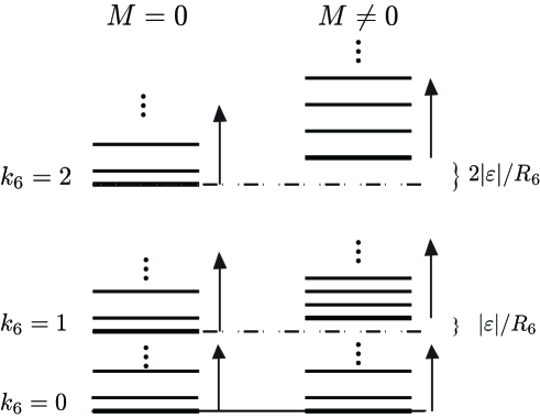
Figure 1: Spectra of massive gauge bosons in a fluxless toroidal compactification (left) and in the fluxed example at hand (right), in the regime $R_{1}R_{2}\gg MR_{6}$. The mass scale introduced by the fluxes is given by $\varepsilon=MR_{6}/\pi R_{1}R_{2}$.

Note that, even if we consider diluted fluxes, there are some qualitative differences in the KK open string spectrum with respect to the fluxless case. In particular, for $k_{6}\neq 0$ the masses of all the excitations along the base $B_{4}$ scale linearly with respect to their KK quantum numbers, whereas in the toroidal case these scale quadratically. In addition, the wavefunctions $|B^{(k,\delta_{1},\delta_{4})}_{n,k_{3},k_{6}}|^{2}$ have a non-constant profile only along two directions, $x^{1}$ and $x^{4}$, as depicted in figure 2 for the first energy levels, reflecting the localization (independently of the warping) of these Kaluza-Klein modes along those directions. Note that the localization of Kaluza-Klein excitations may affect in an interesting way the effective supergravity description, leading to suppressions in the couplings of these modes to the low energy effective theory.

Figure 2: $|B^{(k,\delta_{1},\delta_{4})}_{n,k_{3},k_{6}}|^{2}$ for $k=0,1$, $k_{6}M=0,1,2$, $n=k$ and arbitrary $\delta_{1},\delta_{4},$ and $k_{3}$, in the plane $x^{i}=0,\ \ i=3\ldots 6$. The normalization has been left unfixed.

Interestingly, the family of wavefunctions (3.16) can be easily understood in terms of ordinary theta functions as follows. First note that for $n=0$ and $k_{6}M>0$ we have

$$B^{(0,\delta_{1},\delta_{4})}_{0,k_{3},k_{6}}=\left(\frac{2|k_{6}M|R_{5}}{R_{1}\ \textrm{Vol}_{{\cal M}_{6}}}\right)^{1/2}\vartheta\left[{-\frac{\delta_{1}}{k_{6}M}\atop 0}\right]\left(k_{6}M\tilde{z}_{1};\ k_{6}M\tilde{\tau}_{1}\right)\ \vartheta\left[{-\frac{\delta_{4}}{k_{6}M}\atop 0}\right]\left(k_{6}M\tilde{z}_{2};\ k_{6}M\tilde{\tau}_{2}\right)\\ \times\textrm{exp}\left[i\pi k_{6}M\left(\frac{\tilde{z}_{1}\textrm{Im }\tilde{z}_{1}}{\textrm{Im }\tilde{\tau}_{1}}+\frac{\tilde{z}_{2}\textrm{Im }\tilde{z}_{2}}{\textrm{Im }\tilde{\tau}_{2}}\right)\right]\textrm{exp}\left[2\pi i(k_{6}x^{6}+k_{3}x^{3})\right]$$ (3.20)

where we have defined a non-standard complex structure

$$\begin{array}[]{ccc}\tilde{z}_{1}=x^{1}+\tilde{\tau}_{1}x^{2}&&\tilde{\tau}_{1}=iR_{2}/R_{1}\\ \tilde{z}_{2}=x^{4}+\tilde{\tau}_{2}x^{5}&&\tilde{\tau}_{2}=iR_{5}/R_{4}\end{array}$$ (3.21)

The higher energy levels corresponding to $n>0$ can then be built by acting with the following raising operators

$$a^{\dagger}_{1}\equiv\hat{\partial}_{1}-i\hat{\partial}_{2}\qquad a^{\dagger}_{2}\equiv\hat{\partial}_{4}-i\hat{\partial}_{5}$$ (3.22)

which act on the wavefunctions (3.16) as

$$a^{\dagger}_{1}B^{(k,\delta_{1},\delta_{4})}_{n,k_{3},k_{6}}=i\sqrt{\frac{k_{6}M(n-k+1)}{\pi R_{1}R_{2}}}B^{(k,\delta_{1},\delta_{4})}_{n+1,k_{3},k_{6}}$$ (3.23)

$$a^{\dagger}_{2}B^{(k,\delta_{1},\delta_{4})}_{n,k_{3},k_{6}}=i\sqrt{\frac{k_{6}M(k+1)}{\pi R_{1}R_{2}}}B^{(k+1,\delta_{1},\delta_{4})}_{n+1,k_{3},k_{6}}$$ (3.24)

Similarly, for $k_{6}M<0$ we should complex conjugate $\tilde{z}_{k},\tilde{\tau}_{k}$ in (3.20) and $a^{\dagger}_{k}$ in (3.22).

Note that the kind of wavefunctions (3.20) are precisely those arising from open string zero modes charged under a constant $U(1)$ field strength $F_{2}$ in toroidal magnetized compactifications [13]. This was indeed expected, as nilmanifolds $\Gamma\backslash{\cal H}_{2p+1}$ based on the Heisenberg manifold are standard examples of $S^{1}\simeq U(1)$ bundles, and so both kind of wavefunctions can be understood mathematically in terms of sections of the same vector bundle. It is amusing, however, to note that the physical origin of the bundle geometry is quite different for these two cases. Indeed, while in [13] the bundle arises from an open string flux $F_{2}$ and the $U(1)$ fiber is not a physical dimension, in the present case the bundle geometry is sourced entirely form closed string fluxes, and all the coordinates of the fibration correspond to the background geometry. This multiple interpretation of the wavefunctions (3.20) could presumably be understood as a particular case of open/closed string duality, where the closed string background (2.46) is dual to a background of magnetized D9-branes. More precisely, one can build a dictionary between both classes of backgrounds as

closed string		open string
$e^{6}$	$\leftrightarrow$	$A$
$x^{6}$	$\leftrightarrow$	$\Lambda$
$F_{3}^{\text{cl}}$	$\leftrightarrow$	$\omega_{3}$

where $F_{3}=F_{3}^{\text{cl}}+\omega_{3}$, $\omega_{3}$ is the Chern-Simons 3-form for the open string gauge bundle and $\Lambda$ the gauge transformation parameter.

To finish our discussion let us comment on the uniqueness of the above solutions. Note in particular that the change of variables in (3.4) is not unique, and one can check that taking different choices for $\dot{x}^{6}$ leads to wavefunctions that are localized along different directions. Again, this fact is not totally unexpected, since similar effects occur in the context of magnetized D-branes in toroidal compactifications [13]. Let us then consider the following change of coordinates

$${\dot{x}}^{6}\equiv x^{6}+\frac{M}{2}(\epsilon_{a}x^{1}x^{2}+\epsilon_{b}x^{4}x^{5})$$ (3.25)

with $\epsilon_{a},\ \epsilon_{b}=\pm 1$. From a group theoretical point of view, this choice of signs are nothing but the four possible manifold polarizations of the 5-dimensional Heisenberg group ${\cal H}_{5}$. Proceeding as we did in the previous sections, we obtain the following set of wavefunctions

$$B^{(k,\delta_{a},\delta_{b})_{\epsilon_{a},\epsilon_{b}}}_{n,k_{3},k_{6}}={\cal N}_{\epsilon_{a}\epsilon_{b}}\sum_{s_{a},s_{b}\in\mathbb{Z}}\psi_{n-k}\left(\frac{\dot{x}^{a}}{\sqrt{2}}\right)\ \psi_{k}\left(\frac{\dot{x}^{b}}{\sqrt{2}}\right)\,e^{2\pi i\left((\delta_{a}+k_{6}Ms_{a})x^{a}+k_{3}x^{3}+(\delta_{b}+k_{6}Ms_{b})x^{b}+k_{6}\dot{x}^{6}\right)}\\ {\cal N}_{\epsilon_{a}\epsilon_{b}}\,=\,\left(\frac{2\pi|k_{6}M|}{\textrm{Vol}_{{\cal M}_{6}}}\frac{R_{1}R_{2}}{R_{a}R_{b}}\right)^{1/2}\quad\quad\quad\quad\quad\quad\quad\quad\quad\quad$$ (3.26)

with

$$\dot{x}^{a} \equiv\begin{cases}\frac{2}{R_{a}}a^{-1/2}(\delta_{a}+k_{6}M(x^{2}+s_{a}))&\textrm{for }\epsilon_{a}=+1\\ \frac{2}{R_{a}}a^{-1/2}(\delta_{a}-k_{6}M(x^{1}-s_{a}))&\textrm{for }\epsilon_{a}=-1\end{cases}$$ (3.27)

$$\dot{x}^{b} \equiv\begin{cases}\frac{2}{R_{b}}a^{-1/2}(\delta_{b}+k_{6}M(x^{5}+s_{b}))&\textrm{for }\epsilon_{b}=+1\\ \frac{2}{R_{b}}a^{-1/2}(\delta_{b}-k_{6}M(x^{4}-s_{b}))&\textrm{for }\epsilon_{b}=-1\end{cases}$$ (3.28)

$$x^{a}\equiv\begin{cases}x^{1}&\textrm{for }\epsilon_{a}=+1\\ x^{2}&\textrm{for }\epsilon_{a}=-1\end{cases}\qquad x^{b}\equiv\begin{cases}x^{4}&\textrm{for }\epsilon_{b}=+1\\ x^{5}&\textrm{for }\epsilon_{b}=-1\end{cases}$$ (3.29)

and an analogous definition to (3.29) for $R_{a,b}$. Note that $\epsilon_{a}=+1\ (-1)$ leads to wavefunctions localized in $x^{1}\ (x^{2})$, whereas $\epsilon_{b}=+1\ (-1)$ leads to wavefunctions localized in $x^{4}\ (x^{5})$. Each choice of polarization, however, leads to a complete set of wavefunctions. Therefore any wavefunction within a given polarization can be expressed as a linear combination of wavefunctions in a different polarization through a discrete Fourier transform [13]. See Appendix D for a more general, formal presentation of manifold polarizations for the case of nilmanifolds.

3.2 Laplace-Beltrami operators for group manifolds

When finding solutions to the equation (3.1) in our previous example, a key ingredient was to impose $\Gamma$-invariance via the ansatz (3.2). While such ansatz is easy to guess either from the identifications (2.50) or from the magnetized D-brane literature, it is a priori not obvious how to formulate such an ansatz for arbitrary twisted tori.

In the following we would like to systematize the procedure above and generalize it to solve the Laplace-Beltrami equation in arbitrary manifolds of the form ${\cal M}_{6}=\Gamma\backslash G$. As we will see, the method described below not only leads automatically to the two families of KK towers (3.16) and (3.18) that we found for ${\cal M}_{6}=\Gamma\backslash(\mathbb{R}\times{\cal H}_{5})$, but also gives a simple group theoretical understanding of their existence in terms of the irreducible representations of $\mathbb{R}\times{\cal H}_{5}$.

In fact, the relation between families of KK modes on ${\cal M}_{6}=\Gamma\backslash G$ and irreducible representations of a group $G$ can be traced back to the mathematical literature that analyzes the spectrum of Laplace-Beltrami operators in group manifolds. Particularly useful for our purposes will be the tools developed in the context of non-commutative harmonic analysis (see e.g. [50, 51]), a field aiming to extend the results of Fourier analysis to non-commutative topological groups.

In order to motivate this approach let us first consider the Laplace eigenvalue problem in the Abelian case ${\cal M}_{n}=\mathbb{Z}^{n}\backslash\mathbb{R}^{n}=T^{n}$. Here the twisted derivative operators $\hat{\partial}_{m}$ are nothing but ordinary derivatives, so (3.1) reduces to

$$\partial_{x^{i}}\partial^{x^{i}}B=-m_{B}^{2}B$$ (3.30)

and the underlying algebra of isometries is Abelian. A standard approach to solve this Laplace equation is to apply Fourier analysis. More precisely, we can apply the Fourier transform

$$\hat{f}_{\vec{\omega}}=\int_{\mathbb{R}^{n}}B(\vec{x})e^{i\vec{\omega}\cdot\vec{x}}d\vec{x}$$ (3.31)

to rewrite (3.30) in the dual space of momenta. We then obtain

$$\int_{\mathbb{R}^{n}}|\vec{\omega}|^{2}\hat{f}_{\vec{\omega}}\,=\,\int_{\mathbb{R}^{n}}m_{B}^{2}\hat{f}_{\vec{\omega}}$$ (3.32)

which easily gives $\hat{f}_{\vec{\omega}}=\delta(\vec{\omega}-\vec{\omega}_{0})$ and $|\vec{\omega}_{0}|^{2}=m_{B}^{2}$. Hence, the eigenfunctions of the Laplace operator correspond to Kaluza-Klein excitations with constant momentum of norm $m_{B}$. Applying the inverse Fourier transform we find that these are given by $B_{\vec{\omega}}(\vec{x})=e^{-i\vec{\omega}_{0}\cdot\vec{x}}$. The eigenfunctions of $\Delta$ are then nothing but the irreducible unitary representations $e^{i\vec{\omega}\cdot\vec{x}}$ of the group $\mathbb{R}^{n}$, which are also the “coefficients” entering the Fourier transform (3.31). Finally, imposing invariance under the compactification lattice $\Gamma=\mathbb{Z}^{n}$ restricts $\vec{\omega}$ to the dual sublattice $2\pi\mathbb{Z}$.

So one interesting observation that we can extract from this example is that the irreducible unitary representations $\pi_{\vec{\omega}}(\vec{x})=e^{i\vec{\omega}\cdot\vec{x}}$ of the Abelian group $G=\mathbb{R}^{n}$ correspond to the eigenfunctions of the Laplace operator. In particular, those which are invariant under the subgroup $\Gamma=\mathbb{Z}^{n}$ are well-defined in the compact quotient $\Gamma\backslash G$, and so describe the KK wavefunctions of $T^{n}$.

Naively, we would expect that some sort of analogous statement can be made for $G$ a non-Abelian group. Again, a good starting point is to consider the non-commutative version of (3.31), which reads [50, 51]

$$\hat{f}_{\vec{\omega}}\,\varphi(\vec{s})=\int_{G}B(g)\pi_{\vec{\omega}}(g)\varphi(\vec{s})dg$$ (3.33)

with $\pi_{\vec{\omega}}(g)$ a complete set of inequivalent irreducible unitary representations of $G$. An important difference with respect to the Abelian case is that the irreducible representations $\pi_{\vec{\omega}}(g)$ are no longer simple functions, but rather operators acting on a Hilbert space of functions, $\varphi(\vec{s})\in L^{2}(\mathbb{R}^{p(\pi)})$ with $p(\pi)\in\mathbb{N}$, and so is $\hat{f}_{\vec{\omega}}$. Remarkably, the set $\pi_{\vec{\omega}}$ can be computed systematically by means of the so-called orbit method, mainly developed by A. Kirillov [53], and which we briefly summarize in Appendix D.

In principle, one could follow the standard strategy of the Abelian case and make use of (3.33) to write down eq.(3.1) in the space of momenta, and then apply the inverse Fourier transform to obtain our wavefunction $B$. An alternative approach, which we will adopt here, is to start with an educated ansatz for $\Gamma$-invariant wavefunctions, based on the close relation between Laplace-Beltrami eigenfunctions and unitary irreps of $G$.

Indeed, consider a complex valued function $B_{\vec{\omega}}:G\rightarrow\mathbb{C}$, defined as

$$B^{\varphi,\psi}_{\vec{\omega}}(g)\,=\,\left(\pi_{\vec{\omega}}(g)\varphi,\psi\right)\,\equiv\,\int_{\mathbb{R}^{p(\pi)}}\bar{\psi}(\vec{s})\cdot[\pi_{\vec{\omega}}(g)\varphi(\vec{s})]\,d\vec{s}$$ (3.34)

where $(\,,\,)$ is the usual $L^{2}(\mathbb{C}^{p(\pi)})$ norm. If ${\cal L}$ is a differential operator acting on the space of wavefunctions $L^{2}(G)$ that can be expressed as a polynomial $P(\{\mathfrak{t}_{a}\})$ of the algebra generators, then it is easy to see that

$${\cal L}\left(\pi_{\vec{\omega}}(g)\varphi,\psi\right)\,=\,\left(\pi_{\vec{\omega}}(g)\pi_{\vec{\omega}}({\cal L})\varphi,\psi\right)$$ (3.35)

where $\pi_{\vec{\omega}}({\cal L})$ is defined in the obvious way [50, 51]. Hence, finding eigenfunctions of ${\cal L}$ reduces to finding eigenfunctions of $\pi_{\vec{\omega}}({\cal L})$ in the auxiliary space $L^{2}(\mathbb{R}^{p(\pi)})$, since $\pi_{\vec{\omega}}({\cal L})\varphi=\lambda\varphi\Rightarrow{\cal L}B^{\varphi,\psi}_{\vec{\omega}}=\lambda B^{\varphi,\psi}_{\vec{\omega}}$. Note that this is independent of our choice of $\psi$, which we can take to be, e.g., a delta function $\delta(\vec{s}-\vec{s}_{0})$. A suitable set of eigenfunctions of ${\cal L}$ is then given by

$$B^{\varphi_{\alpha}}_{\vec{\omega}}(g)\,=\,\pi_{\vec{\omega}}(g)\varphi_{\alpha}(\vec{s}_{0})$$ (3.36)

where $\varphi_{\alpha}$ is an eigenfunction of $\pi_{\vec{\omega}}({\cal L})$. In particular, this result applies to the Laplace-Beltrami operator $\Delta$, which can be written as a quadratic form on $\{\mathfrak{t}_{a}\}$. Hence, (3.36) provides a clear correspondence between unitary irreps of $G$ and families of eigenfunctions of its Laplace-Beltrami operator.

As stressed before, we also need to impose that our wavefunctions are well-defined in the quotient space ${\cal M}=\Gamma\backslash G$. A simple way to proceed is to consider the sum

$$B_{\vec{\omega}}(g)\,=\,\sum_{\gamma\in\Gamma}\pi_{\vec{\omega}}(\gamma g)\varphi(\vec{s}_{0})\,\equiv\,\pi_{\vec{\omega}}^{\Gamma}(g)\varphi(\vec{s}_{0})$$ (3.37)

keeping only the wavefunctions $B_{\vec{\omega}}$ belonging to $L^{2}({\cal M})$. Again, if $\varphi$ is an eigenfunction of $\pi_{\vec{\omega}}({\cal L})$ then (3.37) is automatically an eigenfunction of $\Delta$. Alternatively, one may consider $\varphi$ an unknown function and the expression (3.37) an educated ansatz to be plugged into the Laplace-Beltrami equation (3.1).

In order to illustrate how this ansatz works, let us again consider the $(2p+1)$ dimensional Heisenberg manifold $\mathcal{H}_{2p+1}$, discussed in Section 2.3. The Stone-von Neumann theorem [50, 51] states that the irreducible unitary representations for $\mathcal{H}_{2p+1}$ are given by two inequivalent sets

$$\pi_{k_{z}^{\prime}}(\vec{X})\,u(\vec{s})\,=\,e^{2\pi ik_{z}^{\prime}[z+\vec{x}\cdot\vec{y}/2+\vec{y}\cdot\vec{s}]}\,u(\vec{s}+\vec{x})\ u(\vec{s}) \in L^{2}(\mathbb{R}^{p})$$ (3.38)

$$\pi_{\vec{k}_{x}^{\prime},\vec{k}_{y}^{\prime}}(\vec{X})\,=\,e^{2\pi i(\vec{k}_{x}^{\prime}\cdot\vec{x}\ +\ \vec{k}_{y}^{\prime}\cdot\vec{y})}$$ (3.39)

where we are taking the same parameterization $\vec{X}^{t}=(z,\vec{x}^{\,t},\vec{y}^{\,t})$ of $\mathcal{H}_{2p+1}$ as in (2.44). Considering the cocompact subgroup $\Gamma_{{\cal H}_{2p+1}}=\{(\vec{x},\vec{y},z)=M(\vec{n}_{x},\vec{n}_{y},n_{z})\in M\mathbb{Z}^{2p+1}\}$, $M\in 2\mathbb{Z}$, and the $\Gamma_{{\cal H}_{2p+1}}$-invariant representations $\pi^{\Gamma}$ we obtain

$$\pi_{k_{z}}^{\Gamma}(\vec{X})\,u(\vec{s})=\sum_{\vec{s}_{x},\vec{s}_{y}\in\mathbb{Z}^{p}}e^{2\pi ik_{z}[z+\frac{M}{2}\vec{x}\cdot\vec{y}+(\vec{y}+\vec{s}_{y})\cdot(\vec{s}+M\vec{s}_{x})]}\,u(\vec{s}+M(\vec{s}_{x}+\vec{x}))\quad\quad\quad k_{z}\in\mathbb{Z}$$ (3.40)

$$\pi_{\vec{k}_{x},\vec{k}_{y}}^{\Gamma}(\vec{X})=e^{2\pi i(\vec{k}_{x}\cdot\vec{x}\ +\ \vec{k}_{y}\cdot\vec{y})}\hskip 206.28247pt\vec{k}_{x},\vec{k}_{y}\in\mathbb{Z}^{p}$$ (3.41)

where as before we have normalized the generators of the algebra as $\tilde{\mathfrak{t}}_{\alpha}=M\mathfrak{t}_{\alpha}$, and in addition we have relabeled the unirreps as $\vec{k}_{a}=M\vec{k}_{a}^{\prime}$, $a=x,y,z$. An interesting effect of considering the invariant unirreps $\pi^{\Gamma}$ is that the allowed choices for $\vec{s}\in\mathbb{R}^{p}$ become discrete. Indeed, note that (3.40) vanishes unless $k_{z}\vec{s}\in\mathbb{Z}^{p}$, and that if we impose the latter condition we no longer need to sum over $\vec{s}_{y}$ to produce an invariant unirrep. Hence, we can identify our set of $\Gamma$-invariant unirreps producing our ansatz (3.37) as

$$\pi_{k_{z}}^{\Gamma}(\vec{X})\,\varphi_{\vec{\delta}}=\sum_{\vec{s}_{x}\in\mathbb{Z}^{p}}e^{2\pi ik_{z}\left(z+\frac{M}{2}\vec{x}\cdot\vec{y}\right)}e^{2\pi i\left(\vec{y}\cdot(\vec{\delta}+k_{z}M\vec{s}_{x})\right)}\varphi(\vec{\delta}+k_{z}M(\vec{s}_{x}+\vec{x}))\quad\quad k_{z}\in\mathbb{Z}$$ (3.42)

$$\pi_{\vec{k}_{x},\vec{k}_{y}}^{\Gamma}(\vec{X})=e^{2\pi i(\vec{k}_{x}\cdot\vec{x}\ +\ \vec{k}_{y}\cdot\vec{y})}\hskip 206.28247pt\vec{k}_{x},\vec{k}_{y}\in\mathbb{Z}^{p}$$ (3.43)

where $\varphi(\vec{s})=u(k_{z}^{-1}\vec{s})$ and $\vec{\delta}\in\mathbb{Z}^{p}$. Note that because of the sum over $\vec{s}_{x}$, for fixed $k_{z}$ there are only $|k_{z}M|^{p}$ independent choices of $\vec{\delta}$ that we can take. Moreover, all these choices can be related via a redefinition of $\vec{x}$, so if we find a solution to the Laplace equation via the ansatz (3.42) in general we will have $|k_{z}M|^{p}$ independent solutions.

To be more concrete, let us go back to the twisted torus example of subsection 2.3.1. Recall that there the internal geometry is given by ${\cal M}_{6}=\Gamma\backslash(\mathbb{R}\times{\cal H}_{5})=S^{1}\times\Gamma_{{\cal H}_{5}}\backslash{\cal H}_{5}$, and that in (3.38) and (3.39) we should take $p=2$ and identify $z\equiv x^{6}$, $\vec{x}\equiv(x^{2},x^{5})$ and $\vec{y}\equiv(x^{1},x^{4})$. The ansatz (3.37) then amounts to take the invariant unirreps (3.42) and (3.43) with the same identifications, and tensored with the unitary irreps of $S^{1}\simeq U(1)$, given by $e^{2\pi ik_{3}x^{3}}$. More precisely we obtain

$$B^{(\delta_{1},\delta_{4})}_{k_{3},k_{6}}(\vec{x})\,=\,\sum_{k_{1},k_{4}}\varphi\left(k_{1}+k_{6}Mx^{2},k_{4}+k_{6}Mx^{5}\right)e^{2\pi i\left(k_{1}x^{1}+k_{3}x^{3}+k_{4}x^{4}+k_{6}\dot{x}^{6}\right)}$$ (3.44)

$$\hskip 142.26378ptk_{i}=\delta_{i}+k_{6}Ms_{i}\quad\quad\quad n_{i}\in\mathbb{Z}$$

$$B_{k_{1},k_{2},k_{3},k_{4},k_{5}}(\vec{x})=\textrm{exp}[2\pi i(k_{1}x^{1}+k_{2}x^{2}+k_{3}x^{3}+k_{4}x^{4}+k_{5}x^{5})]$$ (3.45)

with $\varphi(x,y)$ a function to be determined. Eq.(3.44) is indeed the ansatz considered in eq.(3.2), while (3.45) gives the set of wavefunctions (3.18) obtained by inspection. Finally, plugging (3.44) into (3.1), directly leads to $\varphi(x,y)=\psi_{k}(\mu_{1}x)\psi_{n-k}(\mu_{2}y)$, with $\mu_{1}^{2}=4\pi k_{6}R_{2}/R_{1}$ and $\mu_{2}^{2}=4\pi k_{6}R_{5}/R_{4}$ reproducing the results of the previous section.

As promised, the ansatz (3.37) gives a direct relation between families of KK modes on ${\cal M}_{6}=\Gamma\backslash G$ and invariant unirreps of $G$. In this respect, note that the inequivalent unirreps of $G={\rm exp\,}\mathfrak{g}$ can be extracted from its Lie algebra $\mathfrak{g}$, given by (2.41). Now, from the 4d effective theory point of view $\mathfrak{g}$ is nothing but the 4d gauge algebra resulting from dimensional reduction of the 10d metric [27]. Hence, we can establish a correspondence between inequivalent unirreps of the 4d gauged isometry algebra and families of eigenfunctions of the internal Laplace-Beltrami operator. Note also that $\mathfrak{g}$ is only part of the full 4d $\mathcal{N}=4$ gauged supergravity algebra, as there are further gauge symmetries arising from dimensional reduction of the 10d $p$-forms. As we will argue below, by making use of the global $SL(2)\times SO(6,6+n)$ symmetry one should be able to extend such correspondence to the full 4d gauged algebra and the full set of massive modes of the untwisted D9-brane sector.

3.3 Non-vanishing $\mu$-terms

Let us now apply the ansatz (3.37) to a more involved background, namely the twisted torus compactification with flux-generated $\mu$-terms of subsection 2.3.2. Again, the wavefunctions for the 4d gauge boson are given by the eigenfunctions of the Laplace-Beltrami operator $\Delta$, and more precisely by the solutions to eq.(3.1), with the twisted derivatives given by (2.49). As before, the first step of the ansatz is to find the set of inequivalent unirreps of the Lie group $G$. This can be done via the orbit method, as shown in Appendix D. We then find four families of irreducible unitary representations associated to the Lie algebra defined by eq.(2.55), given in eqs.(D.20)-(D.23).

As a second step, we need to impose $\Gamma$-invariance on these unirreps. For this purpose it is useful to introduce the variables

$$\dot{x}^{3}=x^{3}-\frac{M_{3}}{2}x^{1}x^{2}\quad\text{and}\quad\dot{x}^{6}=x^{6}-\frac{M_{6}}{2}x^{5}x^{1}$$ (3.46)

so that the action of $\Gamma$, given by (2.50), now reads

$$x^{1}\to x^{1}+1\quad\quad\dot{x}^{3}\to\dot{x}^{3}-M_{3}x^{2}\quad\quad\dot{x}^{6}\to\dot{x}^{6}-M_{6}x^{5}$$ (3.47)

with all the other coordinates being periodic, $x^{i}\to x^{i}+1$ for $i=2,4,5$, and $\dot{x}^{i}\to\dot{x}^{i}+1$ for $i=3,6$. Imposing invariance of (D.20)-(D.23) under (3.47) and plugging the result into (3.1), leads to the following $6\times 4=24$ towers of KK gauge boson wavefunctions:

Modes not excited along the fiber $\{\dot{x}^{3},\dot{x}^{6}\}$

These are given by standard toroidal wavefunctions in the base

$$B_{k_{1},k_{2},k_{4},k_{5}}=e^{2\pi i(k_{1}x^{1}+k_{2}x^{2}+k_{4}x^{4}+k_{5}x^{5})}$$ (3.48)

with mass eigenvalue

$$m_{B}^{2}=\sum_{a=1,2,4,5}\left(\frac{k_{a}}{R_{a}}\right)^{2}$$ (3.49)

In particular, this includes the massless gauge boson.

Modes excited along $\dot{x}^{r}$, with $r=3$ or $6$

Their wavefunction is given by

$$B^{(\delta)}_{k_{r},k_{4},k_{8-r},n}\,=\,{\cal N}\,\sum_{s\in\mathbb{Z}}\psi_{n}\left(\frac{\dot{x}^{1}}{\sqrt{2}}\right)e^{2\pi i\left(k_{r}\dot{x}^{r}+k_{4}x^{4}+k_{8-r}x^{8-r}+(\delta+sk_{r}M_{r})x^{r-1}\right)}$$ (3.50)

with $\delta=0\ldots k_{r}M_{r}-1$ and where $\varepsilon_{\mu}\equiv{M_{3}R_{3}}/{2\pi R_{1}R_{2}}$ stands for the mass scale of the flux

$${\cal N}=\left(\frac{2\pi R_{1}}{\textrm{Vol}_{{\cal M}_{6}}}\sqrt{\frac{|k_{r}\varepsilon_{\mu}|}{R_{r}}}\right)^{1/2}\quad\quad\dot{x}^{1}\equiv 2\pi R_{1}\left(\frac{2|\varepsilon_{\mu}k_{r}|}{R_{r}}\right)^{1/2}\left(x^{1}-s-\frac{\delta}{k_{r}M_{r}}\right)$$ (3.51)

The corresponding mass eigenvalues are

$$m_{B}^{2}=\frac{|\varepsilon_{\mu}k_{r}|}{R_{r}}(2n+1)\,+\sum_{a=r,4,8-r}\left(\frac{k_{a}}{R_{a}}\right)^{2}$$ (3.52)

Modes excited along both $\dot{x}^{3}$ and $\dot{x}^{6}$

The wavefunctions for these modes are

$$B^{(\delta_{2},\delta_{5})}_{k_{3},k_{4},k_{6},n}={\cal N}\,\sum_{s\in\mathbb{Z}}\psi_{n}\left(\frac{\dot{x}^{1}}{\sqrt{2}}\right)\,e^{2\pi i\left[k_{4}x^{4}+k_{3}\dot{x}^{3}+k_{6}\dot{x}^{6}+(\delta_{5}+sk_{6}M_{6})x^{5}+(\delta_{2}+sk_{3}M_{3})x^{2}\right]}$$ (3.53)

with

$${\cal N}=\left(\frac{2\pi R_{1}\sqrt{\Delta_{k_{3},k_{6}}|\varepsilon_{\mu}|}}{\textrm{Vol}_{{\cal M}_{6}}}\right)^{1/2}\quad\quad\dot{x}^{1}\equiv 2\pi(2\Delta_{k_{3},k_{6}}|\varepsilon_{\mu}|)^{1/2}R_{1}\left(x^{1}-s-\frac{\delta_{2}}{k_{3}M_{3}}\right)$$ (3.54)

$$\Delta_{k_{3},k_{6}}^{2}\equiv\left(\frac{k_{3}}{R_{3}}\right)^{2}+\left(\frac{k_{6}}{R_{6}}\right)^{2}$$ (3.55)

and where $\delta_{2},\delta_{5}\in\mathbb{Z}$ are related through the constraint $k_{6}\delta_{2}M_{6}=\delta_{5}k_{3}M_{3}$. Finally, the mass eigenvalues are

$$m_{B}^{2}=\Delta_{k_{3},k_{6}}^{2}+\left(\frac{k_{4}}{R_{4}}\right)^{2}+|\varepsilon_{\mu}|\Delta_{k_{3},k_{6}}(2n+1)$$ (3.56)

4 Scalar wavefunctions

In this section we proceed with the computation of the wavefunctions for the 4d scalar modes transforming in the adjoint representation of the gauge group $G_{unbr}$. These modes arise from the term $b^{m}(x^{\mu})\xi^{m}(x^{i})$ in the dimensional reduction (2.13) of the 10d gauge boson, so they can be thought as Wilson line moduli of the compactification plus their KK replicas. Note that the choice of expansion (2.13) in terms of the left-invariant 1-forms $e^{m}$ indeed simplifies the computation of the wavefunctions $\xi^{m}(x^{i})$ which, just as the previous gauge boson wavefunction $B(x^{i})$, are invariant under the action of the subgroup $\Gamma$ in ${\cal M}_{6}=\Gamma\backslash G$.

In fact, we will see that having computed the spectrum of $B(x^{i})$’s, the computation of $\xi^{m}(x^{i})$’s reduces to a purely algebraic problem. This problem is easily solved in the case of our compactification with vanishing $\mu$-terms, since it basically amounts to diagonalize a $3\times 3$ matrix with commuting entries. The case with non-vanishing $\mu$-term, on the other hand, turns out to be more involved, as the entries of this $3\times 3$ matrix become non-commutative.

4.1 Vanishing $\mu$-terms

As discussed in Section 2.2, for elliptic fibrations of the form (2.28) the internal profiles $\xi^{p}_{\Pi_{2},B_{4}}$ of the 4d scalars in the adjoint of $G_{unbr}$ are real functions satisfying eqs.(2.36) and (2.37). These equations of motion can be summarized in matrix notation as

$$\left[\mathbb{M}+m_{b}^{2}\ \mathbb{I}_{6}\right]\mathbb{V}=0$$ (4.1)

where

$$\mathbb{V}=\begin{pmatrix}\xi^{1}\\ \xi^{2}\\ \xi^{3}\\ \xi^{*\,1}\\ \xi^{*\,2}\\ \xi^{*\,3}\end{pmatrix}\quad\quad\quad\begin{array}[]{c}\xi^{1}\,\equiv\,\xi_{B_{4}}^{1}+i\xi_{B_{4}}^{4}\\ \xi^{2}\,\equiv\,\xi_{B_{4}}^{2}+i\xi_{B_{4}}^{5}\\ \xi^{3}\,\equiv\,\xi_{\Pi_{2}}^{3}+i\xi_{\Pi_{2}}^{6}\end{array}\quad\quad\quad\begin{array}[]{c}\xi^{*\,1}\,\equiv\,\xi_{B_{4}}^{1}-i\xi_{B_{4}}^{4}\\ \xi^{*\,2}\,\equiv\,\xi_{B_{4}}^{2}-i\xi_{B_{4}}^{5}\\ \xi^{*\,3}\,\equiv\,\xi_{\Pi_{2}}^{3}-i\xi_{\Pi_{2}}^{6}\end{array}$$ (4.2)

and the matrix $\mathbb{M}$ has as entries differential operators whose general expression is given in Appendix E. For the type I vacuum of subsection 2.3.1, one can check that $\mathbb{M}$ reduces to

$$\mathbb{M}\,=\,\begin{pmatrix}\hat{\partial}_{m}\hat{\partial}^{m}&-\varepsilon\hat{\partial}_{6}&0&0&0&0\\ \varepsilon\hat{\partial}_{6}&\hat{\partial}_{m}\hat{\partial}^{m}&0&0&0&0\\ 0&0&\hat{\partial}_{m}\hat{\partial}^{m}&0&0&0\\ 0&0&0&\hat{\partial}_{m}\hat{\partial}^{m}&-\varepsilon\hat{\partial}_{6}&0\\ 0&0&0&\varepsilon\hat{\partial}_{6}&\hat{\partial}_{m}\hat{\partial}^{m}&0\\ 0&0&0&0&0&\hat{\partial}_{m}\hat{\partial}^{m}\end{pmatrix}$$ (4.3)

where as before $\varepsilon=MR_{6}/\pi R_{1}R_{2}$ is the flux scale. Note that all the entries of the matrix $\mathbb{M}$ commute, and so (4.1) can be treated as an ordinary eigenvalue problem. Moreover, $\mathbb{M}$ is block diagonal, with no entries mixing holomorphic and antiholomorphic states. This can be traced back to the fact that our compactification manifold ${\cal M}_{6}$ is complex, as required by $\mathcal{N}=1$ supersymmetry. Therefore, it is enough to solve for one of the $3\times 3$ blocks in (4.3).

In order to do so let us distinguish again between states which are excited along the fiber coordinate $x^{6}$ and states which are not excited along it. For the latter the wavefunction should not depend on $x^{6}$, and so they are annihilated by $\hat{\partial}_{6}$. Therefore, for those states $\mathbb{M}$ is proportional to the Laplace-Beltrami operator, whose eigenvalues were solved for in Section 3.1. It is then straightforward to verify that the wavefunctions associated with these modes are given by the same functions $B_{k_{1},k_{2},k_{3},k_{4},k_{5}}$ defined in equation (3.18). Similarly, the mass eigenvalues are

$$m_{\xi}^{2}=\sum_{i=a}^{5}\left(\frac{k_{a}}{R_{a}}\right)^{2}$$

so the wavefunction $B_{0,0,0,0,0}=const.$ corresponds to the six real Wilson line moduli.

On the other hand, $\hat{\partial}_{6}$ does not act trivially on modes excited along the fiber, as they depend on $x^{6}$. Note however that $\hat{\partial}_{6}$ belongs to the center of the Lie algebra $\mathfrak{g}$ of our twisted torus ${\cal M}_{6}=\Gamma\backslash G$. Hence, $\hat{\partial}_{6}$ commutes with the Laplace-Beltrami operator $\hat{\partial}_{m}\hat{\partial}^{m}$, and so they can be simultaneously diagonalized. In fact, it turns out that the family of wavefunctions (3.16) obtained above are not only eigenfunctions of $\hat{\partial}_{m}\hat{\partial}^{m}$ but also of $\hat{\partial}_{6}$, their eigenvalue for the latter being $ik_{6}/R_{6}$. This allows to diagonalize the upper $3\times 3$ block of (4.3) for the fiber KK modes as

$$(\xi_{\pm})_{n,k_{3},k_{6}}^{(k,\delta_{1},\delta_{4})}\equiv\begin{pmatrix}1\\ \pm i\\ 0\end{pmatrix}B_{n,k_{3},k_{6}}^{(k,\delta_{1},\delta_{4})}$$ (4.4)

with mass eigenvalue

$$m^{2}_{\xi_{\pm}}\,=\,\frac{|\varepsilon k_{6}|}{R_{6}}\left(n+1\mp s_{k_{6}M}\right)+\Delta^{2}_{k_{3},k_{6}}$$ (4.5)

where $s_{k_{6}M}=\text{sign}(k_{6}M)$ and $\Delta_{k_{3},k_{6}}$ is given by (3.55). The effect of the off-diagonal entries in (4.3) is then to shift up or down the mass eigenvalues with respect to the ones computed in Section 3.1 for the gauge bosons. In figure 3 we have represented the splitting of the Laplace-Beltrami energy levels due to this mass shift effect.

The remaining eigenvector is

$$(\xi_{3})_{n,k_{3},k_{6}}^{(k,\delta_{1},\delta_{4})}\equiv\begin{pmatrix}0\\ 0\\ 1\end{pmatrix}B_{n,k_{3},k_{6}}^{(k,\delta_{1},\delta_{4})}$$ (4.6)

with mass eigenvalue

$$m^{2}_{\xi_{3}}\,=\,\frac{|\varepsilon k_{6}|}{R_{6}}(n+1)+\Delta^{2}_{k_{3},k_{6}}$$ (4.7)

identical to the KK masses of the corresponding massive gauge boson. In fact, the degrees of freedom coming from (4.6) should be seen as the extra polarizations that massive gauge bosons have with respect to massless ones.

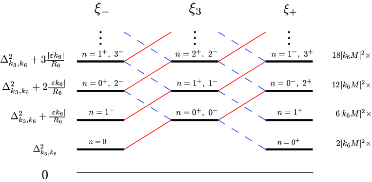
Figure 3: Mass spectra for the complex scalar modes $\xi_{3}$ and $\xi_{\pm}$ excited along the fiber with same momentum $|k_{6}|$ in the example with vanishing $\mu$-terms. Continuous red lines relate states with same $n$ and $k_{6}<0$, whereas dashed blue lines relate states with same $n$ and $k_{6}>0$. We have labeled the energy levels by $n^{s_{k_{6}M}}$. The spectrum of gauge boson excitations coincide with the one of $\xi_{3}$. The flux mass scale is given by $\varepsilon=\frac{MR_{6}}{\pi R_{1}R_{2}}$, whereas $\Delta_{k_{3},k_{6}}^{2}$ is defined in (3.55). We have also indicated the number of real scalars at each energy level, for fixed $s_{k_{6}}$, $s_{k_{3}}$.

Putting these results together with the spectrum of gauge bosons computed in Section 3.1, and the fermionic spectrum (to be computed in next section), one can observe that the content of massive Kaluza-Klein replicas can be arranged into $\mathcal{N}=4$ vector multiplets, except for the levels $k_{6}\neq 0$, $n=0$, which only fit into ultrashort $\mathcal{N}=2$ hypermultiplets. See Section 7.1 for a more detailed discussion.

4.2 Non-vanishing $\mu$-terms

Let us now turn to the type I vacuum of subsection 2.3.2, where the background induces a non-vanishing mass term for one of the chiral multiplets. The internal profiles of the adjoint scalars must again satisfy the eigenvalue problem (4.1), now with $\mathbb{M}$ given by

$$\mathbb{M}=\begin{pmatrix}\hat{\partial}_{m}\hat{\partial}^{m}&-\varepsilon_{\mu}\hat{\partial}_{z^{3}}&-\varepsilon_{\mu}\hat{\partial}_{z^{2}}&0&0&0\\ \varepsilon_{\mu}\hat{\partial}_{\bar{z}^{3}}&\hat{\partial}_{m}\hat{\partial}^{m}&\varepsilon_{\mu}\hat{\partial}_{z^{1}}&0&0&0\\ \varepsilon_{\mu}\hat{\partial}_{\bar{z}^{2}}&-\varepsilon_{\mu}\hat{\partial}_{\bar{z}^{1}}&\hat{\partial}_{m}\hat{\partial}^{m}-\varepsilon_{\mu}^{2}&0&0&0\\ 0&0&0&\hat{\partial}_{m}\hat{\partial}^{m}&-\varepsilon_{\mu}\hat{\partial}_{\bar{z}^{3}}&-\varepsilon_{\mu}\hat{\partial}_{\bar{z}^{2}}\\ 0&0&0&\varepsilon_{\mu}\hat{\partial}_{z^{3}}&\hat{\partial}_{m}\hat{\partial}^{m}&\varepsilon_{\mu}\hat{\partial}_{\bar{z}^{1}}\\ 0&0&0&\varepsilon_{\mu}\hat{\partial}_{z^{2}}&-\varepsilon_{\mu}\hat{\partial}_{z^{1}}&\hat{\partial}_{m}\hat{\partial}^{m}-\varepsilon_{\mu}^{2}\end{pmatrix}$$ (4.8)

with $\varepsilon_{\mu}\equiv M_{3}R_{3}/2\pi R_{1}R_{2}$ and where the complexification

$$\hat{\partial}_{z^{k}}\equiv\hat{\partial}_{k}-i\hat{\partial}_{k+3}$$ (4.9)

is related to the standard choice of complex structure $z^{k}=x^{k}+i(R_{k+3}/R_{k})x^{k+3}$. Note that again the mass matrix is block diagonal, as expected for a 4d SUSY vacuum. We will thus solve (4.1) for the upper block and obtain the other eigenfunctions by complex conjugation.

An important qualitative difference with the case of vanishing $\mu$-term (4.3), is that the entries of the matrix $\mathbb{M}$ are operators that no longer commute. However, using the following commutation relations

$$[\hat{\partial}_{z^{1}},\hat{\partial}_{z^{2}}]\,=\,[\hat{\partial}_{\bar{z}^{1}},\hat{\partial}_{z^{2}}]\,=\,-\varepsilon_{\mu}\hat{\partial}_{z^{3}}\qquad\quad[\hat{\partial}_{z^{1}},\hat{\partial}_{\bar{z}^{2}}]\,=\,[\hat{\partial}_{\bar{z}^{1}},\hat{\partial}_{\bar{z}^{2}}]\,=\,-\varepsilon_{\mu}\hat{\partial}_{\bar{z}^{3}}$$ (4.10)

$$[\hat{\partial}_{m}\hat{\partial}^{m},\hat{\partial}_{z^{2}}]\,=\,-\varepsilon_{\mu}\hat{\partial}_{z^{3}}(\hat{\partial}_{z^{1}}+\hat{\partial}_{\bar{z}^{1}})\qquad[\hat{\partial}_{m}\hat{\partial}^{m},\hat{\partial}_{\bar{z}^{2}}]\,=\,-\varepsilon_{\mu}\hat{\partial}_{\bar{z}^{3}}(\hat{\partial}_{z^{1}}+\hat{\partial}_{\bar{z}^{1}})$$

$$[\hat{\partial}_{m}\hat{\partial}^{m},\hat{\partial}_{z^{1}}]\,=\,[\hat{\partial}_{m}\hat{\partial}^{m},\hat{\partial}_{\bar{z}^{1}}]\,=\,\varepsilon_{\mu}\left(\hat{\partial}_{\bar{z}^{2}}\hat{\partial}_{z^{3}}+\hat{\partial}_{z^{2}}\hat{\partial}_{\bar{z}^{3}}\right)$$

one can still diagonalize this matrix. Indeed, after some little effort one can check that the above system have a complex eigenvector

$$\xi_{3}\equiv\begin{pmatrix}\hat{\partial}_{\bar{z}^{1}}\\ \hat{\partial}_{\bar{z}^{2}}\\ \hat{\partial}_{\bar{z}^{3}}\end{pmatrix}B(\vec{x})$$ (4.11)

with mass eigenvalue $m^{2}_{\xi_{3}}=m_{B}^{2}$, and two complex eigenvectors

$$\xi_{\pm}\equiv\begin{pmatrix}\hat{\partial}_{z^{3}}\hat{\partial}_{\bar{z}^{1}}+m_{\xi_{\pm}}\hat{\partial}_{z^{2}}\\ \hat{\partial}_{z^{3}}\hat{\partial}_{\bar{z}^{2}}-m_{\xi_{\pm}}\hat{\partial}_{z^{1}}\\ \hat{\partial}_{z^{3}}\hat{\partial}_{\bar{z}^{3}}+m_{\xi_{\pm}}^{2}\end{pmatrix}B(\vec{x})$$ (4.12)

with mass eigenvalues

$$m_{\xi_{\pm}}^{2}-\varepsilon_{\mu}m_{\xi_{\pm}}-m_{B}^{2}=0\quad\Longrightarrow\quad m_{\xi_{\pm}}^{2}=\frac{1}{4}\left(\varepsilon_{\mu}\pm\sqrt{\varepsilon_{\mu}^{2}+4m_{B}^{2}}\right)^{2}$$ (4.13)

Here $B(\vec{x})$ is any of the gauge boson wavefunctions (3.48), (3.50) or (3.53) with mass $m_{B}^{2}$ given respectively by eqs.(3.49), (3.52) and (3.56). Hence, for each Kaluza-Klein boson with mass $m_{B}^{2}$, there is one complex scalar with the same mass (eaten by the massive gauge boson via a Higgs mechanism) and two complex scalars whose masses are solutions to the quadratic equation in (4.13).

Note that for the lowest modes of the neutral gauge boson, $B=\textrm{const.}$, the eigenvector parametrization (4.11) and (4.12) breaks down, and does not constitute a good representation of the lightest modes for the scalar fields. Instead, these states correspond to the constant eigenvectors

$$(\xi_{\pm})_{0}\equiv\begin{pmatrix}1\\ \pm i\\ 0\end{pmatrix}\times\text{const.}\qquad(\xi_{3})_{0}\equiv\begin{pmatrix}0\\ 0\\ 1\end{pmatrix}\times\text{const.}$$ (4.14)

with masses $m_{\xi_{\pm}}^{2}=0$ and $m_{\xi_{3}}^{2}=\varepsilon_{\mu}^{2}$, respectively, recovering in this way the low energy effective supergravity result [11]. We will come back to this point in Section 7.2.

5 Fermionic wavefunctions

Let us now turn to the equation (2.31) describing the wavefunctions of fermionic eigenmodes. As in the two previous sections, we will consider those modes transforming in the adjoint representation of the unbroken gauge group $G_{unbr}$, computing them explicitly for the two examples of Section 2.3. In general, for compactifications preserving 4d ${\cal N}=1$ supersymmetry, one expects all those modes belonging to the same supermultiplet to share the same internal wavefunction. This should in particular apply to the two type I vacua examples analyzed above, and so the eigenvalue problem for fermionic modes should reduce to the one already solved in Sections 3 and 4. We will see that this is indeed the case. Let us however stress that, as our approach treats bosons and fermions independently, the method below could also be applied to type I backgrounds where the flux breaks 4d supersymmetry and so wavefunctions no longer match. An example of such ${\cal N}=0$ flux vacuum is discussed in Appendix C, where both classes of open string wavefunctions are computed.

Following the conventions of Appendix A, we can take our wavefunction as a linear combination of the fermionic basis (A.7). Defining the vector

$$\Psi\,=\,\left(\begin{array}[]{c}\psi^{0}\\ \psi^{1}\\ \psi^{2}\\ \psi^{3}\end{array}\right)$$ (5.1)

it is then easy to see that (2.31) can be expressed as

$$i({\bf D}+{\bf F})\Psi\,=\,m_{\chi}\Psi^{*}$$ (5.2)

where

$${\bf D}\,=\,\left(\begin{array}[]{cccc}0&\hat{\partial}_{{z}^{1}}&\hat{\partial}_{{z}^{2}}&\hat{\partial}_{{z}^{3}}\\ -\hat{\partial}_{{z}^{1}}&0&-\hat{\partial}_{\bar{z}^{3}}&\hat{\partial}_{\bar{z}^{2}}\\ -\hat{\partial}_{{z}^{2}}&\hat{\partial}_{\bar{z}^{3}}&0&-\hat{\partial}_{\bar{z}^{1}}\\ -\hat{\partial}_{{z}^{3}}&-\hat{\partial}_{\bar{z}^{2}}&\hat{\partial}_{\bar{z}^{1}}&0\end{array}\right)$$ (5.3)

and ${\bf F}$ contains the contribution of the term proportional to $\not{f}$ in eq.(2.31). In particular, we have that ${\bf F}=0$ for vanishing $\mu$-terms.

Eq.(5.2) implies that

$$({\bf D}+{\bf F})^{*}({\bf D}+{\bf F})\Psi\,=\,|m_{\chi}|^{2}\Psi$$ (5.4)

which is the fermionic equivalent to (4.1).

5.1 Vanishing $\mu$-terms

Let us then consider the internal Dirac equation in the vanishing $\mu$-term background of subsection 2.3.1. First, given the choice of fibration and the conventions of Appendix A, the splitting (2.33) reads

$$\chi_{\Pi_{2}}\,=\,\psi^{0}\,\chi_{---}+\psi^{3}\,\chi_{++-}$$ (5.5)

$$\chi_{B_{4}}\,=\,\psi^{1}\,\chi_{-++}+\psi^{2}\,\chi_{+-+}$$ (5.6)

Second, recall that the contraction of indices in (2.25) and (2.31) is performed with the internal gamma matrices in (A.9), which are essentially the 6d matrices in (A.3). Then, the contribution of the geometric flux to the Dirac equation (2.31) reads

$$\not{f}\,=\,\frac{MR_{6}}{2\pi}\left(\frac{\tilde{\gamma}^{126}}{R_{1}R_{2}}+\frac{\tilde{\gamma}^{456}}{R_{4}R_{5}}\right)\,=\,(2\pi)^{-1}\frac{MR_{6}}{R_{1}R_{2}}\left(\tilde{\gamma}^{126}+\tilde{\gamma}^{456}\right)$$ (5.7)

where we have used the condition $R_{1}R_{2}=R_{4}R_{5}$. In addition we have that

$$\tilde{\gamma}^{126}+\tilde{\gamma}^{456}\,=\,-i\left(\sigma_{1}\otimes\sigma_{2}-\sigma_{2}\otimes\sigma_{1}\right)\otimes\sigma_{2}\,=\,\frac{1}{2}\left(\sigma_{z}\otimes\sigma_{\bar{z}}-\sigma_{\bar{z}}\otimes\sigma_{z}\right)\otimes\sigma_{2}$$ (5.8)

where

$$\sigma_{z}\,=\,\left(\begin{array}[]{cc}0&2\\ 0&0\end{array}\right)\quad\quad\quad\sigma_{\bar{z}}\,=\,\left(\begin{array}[]{cc}0&0\\ 2&0\end{array}\right)$$ (5.9)

Hence, we see that $\not{f}\chi_{\Pi_{2}}\equiv\not{f}P_{+}^{\Pi_{2}}\chi=0$, and so ${\bf F}=0$, as expected from the fact that in this background no $\mu$-term is generated for D9-brane moduli.

In order to solve the squared Dirac equation (5.4) we just need to compute the action of ${\bf D}^{*}{\bf D}$, which in general reads

$$\begin{array}[]{c}-{\bf D}^{*}{\bf D}\,=\,\hat{\partial}_{m}\hat{\partial}^{m}\,\mathbb{I}_{4}\,+\\ \sum_{a}\left(\begin{array}[]{cccc}\frac{1}{2}(f_{1\bar{1}}^{a}+f_{2\bar{2}}^{a}+f_{3\bar{3}}^{a})&f_{\bar{2}\bar{3}}^{a}&f_{\bar{3}\bar{1}}^{a}&f_{\bar{1}\bar{2}}^{a}\\ f_{{3}{2}}^{a}&\frac{1}{2}(f_{1\bar{1}}^{a}-f_{2\bar{2}}^{a}-f_{3\bar{3}}^{a})&f_{{2}\bar{1}}^{a}&f_{{3}\bar{1}}^{a}\\ f_{{1}{3}}^{a}&f_{{1}\bar{2}}^{a}&\frac{1}{2}(-f_{1\bar{1}}^{a}+f_{2\bar{2}}^{a}-f_{3\bar{3}}^{a})&f_{{3}\bar{2}}^{a}\\ f_{{2}{1}}^{a}&f_{{1}\bar{3}}^{a}&f_{{2}\bar{3}}^{a}&\frac{1}{2}(-f_{1\bar{1}}^{a}-f_{2\bar{2}}^{a}+f_{2\bar{3}}^{a})\\ \end{array}\right)\hat{\partial}_{a}\end{array}$$

and that for the case at hand reduces to

$$-{\bf D}^{*}{\bf D}\,=\,\left(\begin{array}[]{cccc}\hat{\partial}_{m}\hat{\partial}^{m}&0&0&0\\ 0&\hat{\partial}_{m}\hat{\partial}^{m}&-\varepsilon\hat{\partial}_{6}&0\\ 0&\varepsilon\hat{\partial}_{6}&\hat{\partial}_{m}\hat{\partial}^{m}&0\\ 0&0&0&\hat{\partial}_{m}\hat{\partial}^{m}\end{array}\right)$$ (5.10)

This operator matrix is block diagonal, and it is easy to see that the upper $1\times 1$ box, containing the Laplace-Beltrami operator, corresponds to the eigenvalue problem for the 4d gaugino and its KK replicas, arising from $\psi_{0}$ in (5.1). The lower $3\times 3$ block, on the other hand, corresponds to the squared Dirac operator for the fermionic superpartners of the 4d scalars, since it exactly matches the $3\times 3$ blocks of (4.3). As the diagonalization of (5.10) proceeds exactly as in Section 4.1, we will not repeat it here.

5.2 Non-vanishing $\mu$-terms

Let us now turn to the type I vacuum with $\mu$-term of subsection 2.3.2. An obvious difference with respect to the case without $\mu$-term is the contribution of the background fluxes to the internal Dirac equation, which now reads

$$\not{f}\,=\,(2\pi)^{-1}\left(\frac{M_{3}R_{3}}{R_{1}R_{2}}\tilde{\gamma}^{123}+\frac{M_{6}R_{6}}{R_{1}R_{5}}\tilde{\gamma}^{156}\right)\,=\,\varepsilon_{\mu}\left(\tilde{\gamma}^{123}+\tilde{\gamma}^{156}\right)$$ (5.11)

where we have again used the condition $M_{3}R_{3}/R_{2}=M_{6}R_{6}/R_{5}$. Hence now we have that

$$\tilde{\gamma}^{123}+\tilde{\gamma}^{156}\,=\,\sigma_{1}\otimes\sigma_{1}\otimes i\sigma_{2}-\sigma_{1}\otimes i\sigma_{2}\otimes\sigma_{1}\,=\,\frac{1}{2}\sigma_{1}\otimes\left(\sigma_{\bar{z}}\otimes\sigma_{z}-\sigma_{z}\otimes\sigma_{\bar{z}}\right)$$ (5.12)

and so $\not{f}$ does not kill $\chi_{\Pi_{2}}$, as expected from a compactification with non-trivial $\mu$-terms. As a result, ${\bf F}$ does not vanish, and we have that

$${\bf D}+{\bf F}\,=\,\left(\begin{array}[]{cccc}0&\hat{\partial}_{{z}^{1}}&\hat{\partial}_{{z}^{2}}&\hat{\partial}_{{z}^{3}}\\ -\hat{\partial}_{{z}^{1}}&0&-\hat{\partial}_{\bar{z}^{3}}&\hat{\partial}_{\bar{z}^{2}}\\ -\hat{\partial}_{{z}^{2}}&\hat{\partial}_{\bar{z}^{3}}&0&-\hat{\partial}_{\bar{z}^{1}}\\ -\hat{\partial}_{{z}^{3}}&-\hat{\partial}_{\bar{z}^{2}}&\hat{\partial}_{\bar{z}^{1}}&\varepsilon_{\mu}\end{array}\right)$$ (5.13)

where $\varepsilon_{\mu}$ is now defined as in (4.8). The r.h.s. of eq.(5.4) then reads

$$-({\bf D}+{\bf F})^{*}({\bf D}+{\bf F})\,=\,\left(\begin{array}[]{cccc}\hat{\partial}_{m}\hat{\partial}^{m}&0&0&0\\ 0&\hat{\partial}_{m}\hat{\partial}^{m}&-\varepsilon_{\mu}\hat{\partial}_{{z}^{3}}&-\varepsilon_{\mu}\hat{\partial}_{{z}^{2}}\\ 0&\varepsilon_{\mu}\hat{\partial}_{\bar{z}^{3}}&\hat{\partial}_{m}\hat{\partial}^{m}&\varepsilon_{\mu}\hat{\partial}_{{z}^{1}}\\ 0&\varepsilon_{\mu}\hat{\partial}_{\bar{z}^{2}}&-\varepsilon_{\mu}\hat{\partial}_{\bar{z}^{1}}&\hat{\partial}_{m}\hat{\partial}^{m}-\varepsilon_{\mu}^{2}\end{array}\right)$$ (5.14)

Note that even in this more involved case, where ${\bf F}\neq 0$, the operator matrix (5.14) is block diagonal, as expected from 4d supersymmetry. Again, we can identify the upper block with the gaugino + KK modes eigenvalue equation and the lower one with that for the 4d holomorphic scalars of Section 4.2. Hence, the diagonalization of (5.14) proceeds exactly as for the bosonic sector of the theory.

6 Matter field wavefunctions

Recall that in our general discussion of Section 2, we considered a gauge subsector $U(N)\subset G_{gauge}$ and a $U(N)$ gauge field (2.11) whose vev broke this gauge symmetry as $U(N)\rightarrow\prod_{i}U(n_{i})\equiv G_{unbr}$. Just like in the more familiar fluxless case [13], from this gauge breaking pattern we obtain 4d fields transforming in the adjoint representation of each $U(n_{i})$ factor, arising from the fluctuations contained in (2.13) and their fermionic partners, as well as 4d fields in the bifundamental representations $({n}_{i},\bar{n}_{j})$, arising from those in (2.14). Up to now we have focused on those open string modes that correspond to $U(n_{i})$ adjoint representations or, otherwise said, on those wavefunctions arising from (2.13). As we have seen, both the mass spectrum and the internal wavefunctions of these modes are directly modified by the closed string background flux $F_{3}$ and by the torsional metric of the compactification manifold ${\cal M}_{6}$.

While this sector of adjoint representation modes already gives us a lot of information on the interplay between open strings and background fluxes, for phenomenological purposes it is clearly not the most interesting one. Indeed, from our recent experience with D-brane model building (see, e.g., [3, 12, 54]) we know that the bifundamental modes arising from (2.14) and their fermionic partners can in principle reproduce the matter content of the MSSM from their lightest modes. Since these light matter fields wavefunctions are crucial to compute effective theory quantities like Yukawa couplings and soft terms, an essential question to be answered is how they are affected in the presence of background fluxes. We will devote this section to obtain the spectrum of bifundamental eigenmodes and eigenfunctions arising from the expansion (2.14), leaving the discussion in terms of 4d effective theory for the next section.

As can be guessed from the magnetized D-brane literature, matter field wavefunctions will not only be affected by closed string fluxes like $F_{3}$, but also by the open string magnetic flux $F_{2}=dA$ under which they are charged. As we will see, the resulting wavefunction can be understood as an open string mode charged under an effective closed + open string magnetic flux, with the relative densities of both kind of fluxes entering the wavefunction in a rather interesting way.

Let us be more precise and let us consider the gauge symmetry breaking $U(N)\to U(p_{\alpha})\times U(p_{\beta})$. In the twisted tori examples of Section 2.3, this breaking will be induced by an open string flux $F_{2}$ with indices on the $T^{2}\times T^{2}$ base of ${\cal M}_{6}$ and of the form

$$F_{2}=2\pi\sum_{k=1,2}\begin{pmatrix}m^{k}_{\alpha}\mathbb{I}_{n_{\alpha}}&0\\ 0&m^{k}_{\beta}\mathbb{I}_{n_{\beta}}\end{pmatrix}\ dx^{k}\wedge dx^{k+3}$$ (6.1)

with $n_{\alpha}+n_{\beta}=N$ and $p_{\Lambda}\equiv g.c.d.(n_{\Lambda},n_{\Lambda}m_{\Lambda}^{1},n_{\Lambda}m_{\Lambda}^{2},n_{\Lambda}m_{\Lambda}^{1}m_{\Lambda}^{2})$, $\Lambda=\alpha,\beta$. For simplicity, we will assume that $n_{\Lambda},m_{\Lambda}^{k}\in\mathbb{Z}$, which in the language of [13] corresponds to a compactification with Abelian Wilson lines.

Given this particular choice of open string flux, we can proceed with our dimensional reduction scheme of eqs.(2.13) and (2.14). Here $\langle B\rangle=\langle B^{\Lambda}\rangle U_{\Lambda}$, where $U_{\Lambda}$ is defined by (2.12) and $\langle B^{\Lambda}\rangle$ can be chosen to be

$$\langle B^{\Lambda}\rangle=\pi\sum_{k=1,2}m_{\Lambda}^{k}[x^{k}dx^{k+3}-x^{k+3}dx^{k}]\qquad\qquad\Lambda=\alpha,\beta$$ (6.2)

where, again for simplicity, we have set all Wilson lines to zero. The gauge transformation of a $U(N)$ adjoint field along a non-trivial closed path $\gamma$ is then

$$W\ \to\ \textrm{exp}\left[i\oint_{\gamma}\langle B^{\Lambda}\rangle U_{\Lambda}\right]\cdot W\cdot\textrm{exp}\left[-i\oint_{\gamma}\langle B^{\Lambda}\rangle U_{\Lambda}\right]$$ (6.3)

so for a $(\bar{n}_{\alpha},{n}_{\beta})$ representation we have

$$x^{k}\to x^{k}+1\ ,\ \ldots\ :\qquad W^{\alpha\beta}\to e^{i\pi I^{k}_{\alpha\beta}x^{k+3}}W^{\alpha\beta}$$ (6.4)

$$x^{k+3}\to x^{k+3}+1\ ,\ \ldots\ :\qquad W^{\alpha\beta}\to e^{-i\pi I^{k}_{\alpha\beta}x^{k}}W^{\alpha\beta}$$

where the dots in the l.h.s. indicate a possible accompanying action on the fiber, as dictated by the structure of our twisted torus ${\cal M}_{6}$ (see e.g. (2.50) or (2.56)), and $k=1,2$. We have also defined $I^{k}_{\alpha\beta}=m^{k}_{\alpha}-m^{k}_{\beta}$, following the conventions in [13].

Finally, consistency with the equations of motion for $F_{2}$ requires that $I^{1}_{\alpha\beta}I^{2}_{\alpha\beta}<0$. Let us in particular assume that $I^{2}_{\alpha\beta}>0>I^{1}_{\alpha\beta}$, and introduce the quantities

$$\sigma_{\pm}=\frac{1}{2\pi}\left(\frac{I^{2}_{\alpha\beta}}{R_{2}R_{5}}\pm\frac{I^{1}_{\alpha\beta}}{R_{1}R_{4}}\right)$$ (6.5)

so that $\sigma_{-}$ is the total density of flux $F_{2}$, whereas $\sigma_{+}$ is proportional to the D-term induced by $F_{2}$ [55]. One can check that the SUSY conditions for $F_{2}$ amount to [56, 57]

$$J^{2}\wedge F_{2}-\frac{1}{3}F_{2}^{3}=J^{2}\wedge F_{2}=0\quad\Leftrightarrow\quad\sigma_{+}=0$$ (6.6)

6.1 W bosons

Let us start considering the 4d vector bosons $w_{\mu}$ in (2.14), transforming in the bifundamental representation of $G_{unbr}=U(n_{\alpha})\times U(n_{\beta})$. The internal profile of such open string mode is given by the scalar wavefunction $W=W^{\alpha\beta}e_{\alpha\beta}$, with components $W^{\alpha\beta}$ satisfying the equation of motion

$$\hat{D}^{m}\hat{D}_{m}W^{\alpha\beta}=-m_{W}^{2}W^{\alpha\beta}$$ (6.7)

with

$$\hat{D}_{m}W^{\alpha\beta}=\hat{\partial}_{m}W^{\alpha\beta}-i(\langle B_{m}^{\alpha}\rangle-\langle B_{m}^{\beta}\rangle)W^{\alpha\beta}$$ (6.8)

in agreement with our notation in eqs.(2.38) and (2.39). Note that (6.7) reduces to (3.1) if we set $\langle B^{\Lambda}\rangle=0$, so it is reasonable to expect a structure of KK modes similar to the one found in Section 3.

In particular, for bosons in the adjoint representation we have seen that KK modes not excited along the fiber do not feel the closed string fluxes at all, and so they present the spectrum of a standard, fluxless toroidal compactification. The same result applies to W bosons, in the sense that if $W^{\alpha\beta}$ does not depend on the coordinates of the fiber $\hat{\partial}$ becomes the standard partial derivative. As a result, (6.7) becomes in this case the equation of motion for a $W$ boson in a magnetized $T^{2}\times T^{2}$, and their spectrum follows from the results in [13]. Indeed, the lightest mode, of mass $m^{2}_{W}=|\sigma_{-}|$, is given by

$$W^{\alpha\beta,\ (0,j_{1},j_{2})}_{0}(\tilde{z}_{1}^{\prime},\tilde{z}_{2}^{\prime})={\cal N}\prod_{k=1,2}e^{i\pi|I^{k}_{\alpha\beta}|\tilde{z}_{k}^{\prime}\textrm{Im }\tilde{z}_{k}^{\prime}/\textrm{Im }\tilde{\tau}_{k}^{\prime}}\ \vartheta\left[{\frac{j_{k}}{|I^{k}_{\alpha\beta}|}\atop 0}\right](|I^{k}_{\alpha\beta}|\tilde{z}_{k}^{\prime}\,{\Large;}\,|I^{k}_{\alpha\beta}|\tilde{\tau}_{k}^{\prime})\\ {\cal N}\,=\,\left(\frac{2}{\textrm{Vol}_{{\cal M}_{6}}}\right)^{1/2}\prod_{k=1,2}(|I^{k}_{\alpha\beta}|\textrm{Im }\tilde{\tau}_{k}^{\prime})^{1/4}\qquad\begin{array}[]{ccc}\tilde{z}_{1}^{\prime}=x^{4}+\tilde{\tau}_{1}^{\prime}x^{1}&&\tilde{\tau}_{1}^{\prime}=iR_{1}/R_{4}\\ \tilde{z}_{2}^{\prime}=x^{2}+\tilde{\tau}_{2}^{\prime}x^{5}&&\tilde{\tau}_{2}^{\prime}=iR_{5}/R_{2}\end{array}$$ (6.9)

where again we have defined a non-standard choice of complex structure. As in [13], a full KK tower can be constructed from (6.9) by applying appropriate raising operators.

On the other hand, for modes with non-vanishing Kaluza-Klein momentum along the fiber, some subtleties arise. Let us for concreteness focus on the example without flux-generated $\mu$-terms of subsection 2.3.1, whose gauge boson spectrum was analyzed in Section 3.1. There, we saw that in practice one can trade the effect of a closed string flux on ${\cal M}_{6}$ by an appropriate magnetic flux $F_{2}^{\text{cl}}=2\pi k_{6}M(dx^{1}\wedge dx^{2}+dx^{4}\wedge dx^{5})$ on the $T^{2}\times T^{2}$ base of the fibration. Since now our W boson also feels the genuine open string flux $(F_{2}^{\alpha\beta})^{\text{op}}=2\pi(I^{1}_{\alpha\beta}dx^{1}\wedge dx^{4}+I^{1}_{\alpha\beta}dx^{2}\wedge dx^{5})$, it is natural to consider a total, effective magnetic flux defined as $(F_{2})_{\text{eff}}=F_{2}^{\text{op}}+F_{2}^{\text{cl}}$, which in this case reads

$$(F^{\alpha\beta}_{2})_{\rm eff}\,=\,2\pi\,dx^{1}\wedge(k_{6}Mdx^{2}+I^{1}_{\alpha\beta}dx^{4})+2\pi\,(k_{6}Mdx^{4}+I^{2}_{\alpha\beta}dx^{2})\wedge dx^{5}$$ (6.10)

and to expect that our open string modes behave as particles charged under $(F_{2})_{\rm eff}$.

In our example, the choice of $T^{2}\times T^{2}$ metric (2.46b), guarantees that both fluxes $F_{2}^{\text{cl}}$ and $F_{2}^{\text{op}}$ are factorizable, in the sense that they can be decomposed as $F_{2}=F_{2}|_{(T^{2})_{i}}+F_{2}|_{(T^{2})_{j}}$, with $(T^{2})_{i}$ and $(T^{2})_{j}$ two orthogonal two-tori. In turn, this property implies that their associated lowest KK mode can be written as a product of two theta functions, which in the case at hand are given by (3.20) for $F_{2}^{\text{cl}}$ and (6.9) for $F_{2}^{\text{op}}$. Note, however, that $(F_{2})_{\text{eff}}=F_{2}^{\text{op}}+F_{2}^{\text{cl}}$ will in general not be factorizable, and so we cannot expect the associated lowest KK mode to be again a product of two Jacobi theta functions, but rather a Riemann $\vartheta$-function [13]. Hence, for matter modes excited along the fiber we would expect a lowest KK mode wavefunction of the form

$$W^{\alpha\beta,\ (j_{1},j_{2})}_{0,0,k_{3},k_{6}}=\mathcal{N}\ e^{i\pi(\mathbf{N}\cdot\vec{z})\cdot(\textrm{Im }\mathbf{\Omega}_{\bf U})^{-1}\cdot\textrm{Im }\vec{z}}\ \vartheta\left[{\vec{j}\atop 0}\right](\mathbf{N}\cdot\vec{z}\,;\,\mathbf{N}\cdot\mathbf{\Omega}_{\bf U})\ e^{2\pi i(k_{3}x^{3}+k_{6}x^{6})}$$ (6.11)

where $\vec{z}\in\mathbb{C}^{2}$, and $\mathbf{N}$ and $\mathbf{\Omega}_{\bf U}$ are $2\times 2$ real and complex matrices, respectively. The definition of the Riemann $\vartheta$-function and its properties can be found in Appendix F.

Indeed, one can check that the ansatz (6.11) is a solution of (6.7), (2.50), (6.4), with mass eigenvalue $m^{2}_{W}=\Delta^{2}_{k_{3},k_{6}}+\rho$, if we set

$$\vec{z}=\begin{pmatrix}x^{4}\\ x^{2}\end{pmatrix}+\mathbf{\Omega}_{\bf U}\cdot\begin{pmatrix}x^{1}\\ x^{5}\end{pmatrix}\quad\qquad\mathbf{\Omega}_{\bf U}=\bar{\bf B}^{-1}\cdot\bar{\bf U}\cdot\bar{\bf B}\cdot\bf{\Omega}$$ (6.12)

and

$$\mathbf{N} =\begin{pmatrix}-I^{1}_{\alpha\beta}&-k_{6}M\\ k_{6}M&I^{2}_{\alpha\beta}\end{pmatrix} \mathbf{\Omega} =i\begin{pmatrix}\frac{R_{1}}{R_{4}}&0\\ 0&\frac{R_{5}}{R_{2}}\end{pmatrix}$$ (6.13)

$$\mathbf{B} =\sqrt{2}\pi\begin{pmatrix}R_{4}&0\\ 0&R_{2}\end{pmatrix} \mathbf{U} =\begin{pmatrix}\textrm{cos }\phi&\textrm{sin }\phi\\ -\textrm{sin }\phi&\textrm{cos }\phi\end{pmatrix}$$ (6.14)

$$\mathcal{N} =\left(\frac{2R_{5}\,{\rm det\,}{\bf N}}{R_{2}\textrm{Vol}_{{\cal M}_{6}}}\right)^{1/2} \vec{j}^{\,t}{\bf N}\in\mathbb{Z}^{2}$$ (6.15)

where we have defined the effective flux density $\rho$ and the interpolation angle $\phi$ as

$$\rho=\sqrt{\rho_{\text{op}}^{2}+\rho_{\text{cl}}^{2}}=\sqrt{\sigma_{-}^{2}+\left(\frac{k_{6}\varepsilon}{R_{6}}\right)^{2}}\quad\qquad\textrm{tan }\phi=\frac{\rho_{\text{cl}}}{\rho_{\text{op}}}=\frac{k_{6}\varepsilon}{R_{6}\sigma_{-}}$$ (6.16)

Note that ${\bf N}$ and ${\bf\Omega}_{\bf U}$ satisfy the convergence conditions (F.21) that allow (6.11) to be well-defined, and that the degeneracy of each level is given by $\textrm{det }\mathbf{N}$. Moreover, under the lattice transformations (2.50a)-(2.50f), $W^{\alpha\beta}$ transforms as dictated by (6.4). Finally, $\phi$ interpolates between the two choices of complex structures (3.21) and (6.9). In the limit $\phi\rightarrow\pi/2$ we recover from (6.12) $z_{k}=\tilde{z}_{k}$ and the factorized wavefunctions (3.20) for neutral bosons, while in the limit $\phi\rightarrow 0$ we obtain $z_{k}=\tilde{z}_{k}^{\prime}$ and the wavefunctions for charged bosons without KK momentum along the fiber, given by (6.9).

In order to build the full tower of Kaluza-Klein excitations for the charged bosons, we can systematically act on (6.11) with the holomorphic covariant derivatives defined in Appendix F, which for the case at hand read

$$a^{\dagger}_{1} \equiv\hat{D}_{2}+i\ \textrm{sin }\phi\,\hat{D}_{1}-i\ \textrm{cos }\phi\,\hat{D}_{5}$$ (6.17)

$$a^{\dagger}_{2} \equiv\hat{D}_{4}-i\ \textrm{cos }\phi\,\hat{D}_{1}-i\ \textrm{sin }\phi\,\hat{D}_{5}$$ (6.18)

Indeed, note that the deformation angle $\phi$ is such that

$$\textrm{Im }{\bf\Omega}_{\bf U}^{-1}\cdot{\bf N}^{t}=(\textrm{Im }{\bf\Omega}^{-1}_{\bf U})^{t}\cdot{\bf N}$$ (6.19)

and as a result $[a_{1}^{\dagger},a_{2}^{\dagger}]=0$. This allows us to write a number operator

$$N=\hat{D}_{m}\hat{D}^{m}+\rho\$$ (6.20)

and to build the full KK tower of states by applying $(a_{1}^{\dagger})^{n-k}(a_{2}^{\dagger})^{k}$ to (6.11). The resulting spectrum of masses is given by

$$m_{W}^{2}=\left(\frac{k_{3}}{R_{3}}\right)^{2}+\left(\frac{k_{6}}{R_{6}}\right)^{2}+(n+1)\rho+(2k-n)\frac{\sigma_{+}\sigma_{-}}{\rho}\quad\qquad k,n\in\mathbb{Z}$$ (6.21)

where $k=0,\ldots,n$.

Interestingly, for a vanishing D-term $\sigma_{+}=0$ the effective flux (6.10) factorizes, and so the Riemann $\vartheta$-function in (6.11) becomes the product of two ordinary $\vartheta$-functions. In that case, the complete tower of wavefunctions is given by

$$W^{\alpha\beta,(k,\delta_{1},\delta_{2})}_{n,k_{3},k_{6}}\,=\,\left(\frac{2\pi\rho R_{1}R_{5}}{\textrm{Vol}_{{\cal M}_{6}}}\right)^{1/2}\sum_{s_{1},s_{2}\in\mathbb{Z}}\psi_{n-k}\left(\frac{\dot{x}^{a}}{\sqrt{2}}\right)\ \psi_{k}\left(\frac{\dot{x}^{b}}{\sqrt{2}}\right)\times$$ (6.22)

$$\times\,\textrm{exp}\left[2\pi i\left((-\delta_{2}-k_{6}Ms_{1}+I^{2}_{\alpha\beta}s_{2})x^{2}+k_{3}x^{3}+(\delta_{1}-I^{1}_{\alpha\beta}s_{1}+k_{6}Ms_{2})x^{4}+k_{6}\dot{x}^{6}\right)\right]$$

with $\delta_{k}=0\ldots\textrm{g.c.d}(k_{6}M,I^{k}_{\alpha\beta})-1$. Note that these wavefunctions have the same structure as in (3.16), but now they localize along the tilted coordinates

$$\dot{x}^{a}\equiv\frac{1}{R_{2}}\sqrt{\frac{4\pi}{\rho}}[\delta_{2}+k_{6}M(x^{1}+s_{1})-I^{2}_{\alpha\beta}(x^{5}+s_{2})]$$

$$\dot{x}^{b}\equiv\frac{1}{R_{4}}\sqrt{\frac{4\pi}{\rho}}[\delta_{1}-I^{1}_{\alpha\beta}(x^{1}+s_{1})+k_{6}M(x^{5}+s_{2})]$$

Alternatively, we could have derived all the above results by considering an extended version of the algebra (2.41), accounting for the D9-brane gauge generators, and then making use of the representation theory methods described in Section 3.2. More precisely, we know that the algebra (2.41) is part of the four dimensional gauge algebra, corresponding to the gauge symmetries which arise from dimensional reduction of the metric tensor. This, however, is not the full 4d gauge algebra. In particular, in the presence of D9-branes, we should also include the generators of the $U(1)$ gauge symmetries arising from such open string sector [27, 58]

$$[\hat{D}_{m},\hat{D}_{n}] =-f^{p}_{mn}\hat{D}_{p}+iF^{\alpha}_{mn}U_{\alpha}$$ (6.23)

$$[\hat{D}_{m},U_{\alpha}] =[U_{\alpha},U_{\beta}]=0$$

where the covariant twisted derivatives $\hat{D}_{m}$ are defined as in (6.8) and the Abelian gauge generators $U_{\alpha}$ by (2.12).

Given such extended algebra, it is straightforward to apply the methods of Section 3.2 and Appendix D to compute its irreducible unitary representations. For the case at hand, we find the following two sets of irreducible unitary representations

$$\pi_{k_{1},k_{2},k_{3},k_{4},k_{5}}=\prod_{r=1}^{5}\textrm{exp}[2\pi ik_{r}x^{r}]$$ (6.24)

$$\pi_{k_{3},k_{6},k_{q}}=\textrm{exp}\left[2\pi i\left(k_{3}x^{3}+k^{\alpha\beta}\left(\textrm{Tr }\Lambda_{\alpha\beta}+I^{2}_{\alpha\beta}x^{2}\left(s_{5}+\frac{x^{5}}{2}\right)-I^{1}_{\alpha\beta}x^{4}\left(s_{1}+\frac{x^{1}}{2}\right)\right)\right)\right.$$

$$\hskip 14.22636pt\left.+k_{6}\left(x^{6}-Mx^{2}\left(s_{1}+\frac{x^{1}}{2}\right)+Mx^{4}\left(s_{5}+\frac{x^{5}}{2}\right)\right)\right]u(s_{1}+x^{1},s_{5}+x^{5})$$ (6.25)

where $u(\vec{s})\in L^{2}(\mathbb{R}^{2})$ and $\textrm{Tr }\Lambda_{\alpha\beta}$ is the trace of the gauge parameter (i.e. the unphysical coordinate in the $U(1)\simeq S^{1}$ D9-brane gauge fibers). Note that there is a new natural quantum number $k^{\alpha\beta}$ which we did not find in our previous analysis.

Plugging now (6.24) and (6.25) into (6.7) we find that, indeed, the unirreps (6.25) with $k^{\alpha\beta}=1$ lead to the matter wavefunction solutions (6.11), as well as the more massive replicas produced by acting with $a_{1}^{\dagger}$, $a_{2}^{\dagger}$. It would then seem that those unirreps in (6.24) with $k^{\alpha\beta}\neq 1$ would not correspond to any physical modes, somehow against the general philosophy of Section 3.2. Let us try to argue that such modes do exist.

First, let us consider the meaning of $k^{\alpha\beta}\in\mathbb{Z}$. If we set $k^{\alpha\beta}=0$, then from (6.24) and (6.25) we recover the vector boson adjoint modes (3.16) and (3.18) of Section 3. Indeed, (6.24) directly correspond to adjoint bosons without Kaluza-Klein momentum along the fiber, given by (3.18), while (6.25) with $k^{\alpha\beta}=0$ correspond to the adjoint bosons with Kaluza-Klein momentum along the fiber, given by (3.16). This is not a surprise since, after all, the KK modes of Section 3 arose from the irreducible unitary representations of a subalgebra of (6.23). What is perhaps more illuminating is the fact that neither of the above subset of modes satisfy eq.(6.7), but rather the Laplace-Beltrami equation (3.1) for a neutral boson. This clearly suggest that the internal differential equation that should be satisfied by an arbitrary wavefunction arising from (6.25) is given by (6.7), but with the gauge covariant derivative defined as

$$\hat{D}_{m}W^{\alpha\beta}=\hat{\partial}_{m}W^{\alpha\beta}-ik^{\alpha\beta}(\langle B_{m}^{\alpha}\rangle-\langle B_{m}^{\beta}\rangle)W^{\alpha\beta}\quad\quad k^{\alpha\beta}\in\mathbb{Z}$$ (6.26)

instead of (6.8). In this sense, the massive modes corresponding to $k^{\alpha\beta}\neq 1$ should be understood as states with $U(1)$ charges $k^{\alpha\beta}(-n_{\alpha},n_{\beta})$, which hence undergo the gauge transformations

$$x^{k}\to x^{k}+1\ ,\ \ldots\ :\qquad W^{\alpha\beta}\to e^{i\pi k^{\alpha\beta}I^{k}_{\alpha\beta}x^{k+3}}W^{\alpha\beta}$$ (6.27)

$$x^{k+3}\to x^{k+3}+1\ ,\ \ldots\ :\qquad W^{\alpha\beta}\to e^{-i\pi k^{\alpha\beta}I^{k}_{\alpha\beta}x^{k}}W^{\alpha\beta}$$

In particular, those states with $k^{\alpha\beta}=-1$ correspond to the bifundamental representation $(n_{\alpha},\bar{n}_{\beta})$, whose wavefunction can be obtained by complex conjugation of (6.11). Finally, those modes with $|k^{\alpha\beta}|>1$ should be non-perturbative in nature, as they cannot arise from the perturbative open string spectrum.

Note that the existence of these exotic non-perturbative charged vector states is not only suggested by the spectrum of unirreps (6.25), but also required by global symmetry arguments. Indeed, the 4d effective action of the untwisted D9-brane sector is given by a $\mathcal{N}=4$ gauged supergravity, whose global symmetry group is $SL(2)\times SO(6,6+N)$, and where $N=n_{\alpha}+n_{\beta}$ is the number of extra vector multiplets coming from $D9$-brane gauge symmetries. The spectrum of 4d particles is therefore naturally arranged in multiplets of this global symmetry. In the particular example at hand, the global symmetry group includes a $\mathbb{Z}_{2}$ generator corresponding to the open/closed string correspondence discussed in Section 3.1. This generator maps neutral bosons with Kaluza-Klein momentum $|k_{6}|>1$ along the fiber to non-perturbative charged bosons with $U(1)$ charge $|k^{\alpha\beta}|>1$. Making use of this global symmetry, we would expect the following masses for the non-perturbative modes

$$m_{W}^{2}=\left(\frac{k_{3}}{R_{3}}\right)^{2}+\left(\frac{k_{6}}{R_{6}}\right)^{2}+(n+1)\rho_{\rm n.p.}+(2k-n)(k^{\alpha\beta})^{2}\frac{\sigma_{+}\sigma_{-}}{\rho_{\rm n.p.}}$$ (6.28)

where

$$\rho_{\rm n.p.}=\sqrt{(k^{\alpha\beta}\sigma_{-})^{2}+\left(\frac{k_{6}\varepsilon}{R_{6}}\right)^{2}}$$ (6.29)

Finally, note that the algebra (6.23) is still not the full four dimensional gauge algebra. There are further gauge symmetries which arise from dimensional reduction of e.g. the RR 2-form. In particular, the RR 3-form fluxes enter as structure constants of the complete 4d algebra [58]. We expect the irreducible unitary representations of the complete four dimensional algebra to encode further untwisted states of the higher dimensional string theory. We leave the exploration of these issues for future work.

Similarly, we can work out the wavefunctions for the charged bosons in the example with non-vanishing $\mu$-term of subsection 2.3.2. In that case, the total effective magnetic flux is given by

$$(F_{2}^{\alpha\beta})_{\rm eff}=2\pi\left(I^{1}_{\alpha\beta}dx^{1}\wedge dx^{4}+I^{2}_{\alpha\beta}dx^{2}\wedge dx^{5}+k_{3}M_{3}dx^{1}\wedge dx^{2}+k_{6}M_{6}dx^{1}\wedge dx^{5}\right)$$ (6.30)

Recall that for this vacuum we should distinguish between bosons with no Kaluza-Klein momentum along the $S^{1}$ fibers, bosons with Kaluza-Klein momentum along only one of the fibers, and bosons with momentum along both of the fibers. We can easily adapt our previous discussion in this section to describe the wavefunctions for the first two types of bosons. Indeed, it is not difficult to see that the wavefunctions for charged bosons without momentum along any fiber are given again by eq.(6.9), whereas the wavefunctions for charged bosons with Kaluza-Klein momentum along only one of the fibers, e.g. $k_{3}\neq 0,\ k_{6}=0$, are given by eq.(6.11) with the same parameters $\vec{z}$, ${\bf\Omega}$ and ${\bf B}$, but with charge matrix, deformation angle and effective flux density given by

$${\bf N}=\begin{pmatrix}-I^{1}_{\alpha\beta}&-k_{3}M_{3}\\ 0&I^{2}_{\alpha\beta}\end{pmatrix}\quad\quad\quad\textrm{tan }\phi=\frac{k_{3}\varepsilon_{\mu}}{R_{3}\sigma_{-}}\quad\quad\quad\rho=\sqrt{\sigma_{-}^{2}+\left(\frac{k_{3}\varepsilon_{\mu}}{R_{3}}\right)^{2}}$$ (6.31)

The set of charged bosons excited along both fibers, with arbitrary $k_{3}$ and $k_{6}$, is however a more involved sector, and in particular does not fall into the class of functions (6.11). This basically comes from the fact that $F_{2}$ has then all the possible components of the form $dx^{1}\wedge dx^{\alpha}$. We refer to the reader to Appendix F for a more precise statement as well as a more detailed discussion of this point.

6.2 Bifundamental scalars and fermions

Just like for adjoint KK modes, the wavefunctions for bifundamental scalars and fermions are easily worked out once that the 4d vector boson wavefunctions are known. Note that these bifundamental KK modes are particularly interesting in semi-realistic flux compactification vacua, since they correspond to the MSSM matter fields and their KK replicas.

As before, let us start our analysis by considering the scalars in the bifundamental. From eqs.(2.38)-(2.39), we see that the corresponding mass matrix can be obtained from the one for adjoint scalars analyzed in Appendix E, by simply replacing twisted derivatives $\hat{\partial}_{m}$ by covariant twisted derivatives $\hat{D}_{m}$, and adding a term proportional to $\langle G_{mp}^{\alpha\beta}\rangle$. In particular, for the example without $\mu$-terms discussed in subsection 2.3.1 we obtain the mass matrix

$$\mathbb{M}=\hat{D}_{m}\hat{D}^{m}\mathbb{I}_{6}+\begin{pmatrix}-\frac{I^{1}_{\alpha\beta}}{\pi R_{1}R_{4}}&-\varepsilon\hat{D}_{6}&0&0&0&0\\ \varepsilon\hat{D}_{6}&-\frac{I^{2}_{\alpha\beta}}{\pi R_{2}R_{5}}&0&0&0&0\\ 0&0&0&0&0&0\\ 0&0&0&\frac{I^{1}_{\alpha\beta}}{\pi R_{1}R_{4}}&-\varepsilon\hat{D}_{6}&0\\ 0&0&0&\varepsilon\hat{D}_{6}&\frac{I^{2}_{\alpha\beta}}{\pi R_{2}R_{5}}&0\\ 0&0&0&0&0&0\end{pmatrix}$$ (6.32)

where again $\varepsilon=MR_{6}/\pi R_{1}R_{2}$ and we are using the conventions of (4.2), with $\xi^{p}_{\Pi_{2},B_{4}}$ now complex functions. Like in the case of adjoint scalars, this matrix is block diagonal, and so it will be enough to diagonalize the upper $3\times 3$ block. Note that both blocks are related by an $\mathcal{N}=2$ R-symmetry transformation. However, it is important to notice that, since we are dealing with charged modes, this transformation takes $\sigma_{+}\to-\sigma_{+}$.

For the upper $3\times 3$ block we find the eigenvectors

$$\Phi_{3}^{\alpha\beta}\equiv\begin{pmatrix}0\\ 0\\ 1\end{pmatrix}W^{\alpha\beta}(\vec{x})$$ (6.33)

with mass eigenvalue $m^{2}_{\Phi_{3}}=m^{2}_{W}$, and with $W^{\alpha\beta}(\vec{x})$ the wavefunction of a charged boson. In addition, we find

$$\Phi_{\pm}^{\alpha\beta}\equiv\begin{pmatrix}\sigma_{-}\mp\rho\\ i\varepsilon\frac{k_{6}}{R_{6}}\\ 0\end{pmatrix}W^{\alpha\beta}(\vec{x})$$ (6.34)

with mass eigenvalues $m^{2}_{\Phi_{\pm}}=m^{2}_{W}+\sigma_{+}\pm\rho$. The R-symmetry conjugates $\bar{\Phi}_{\pm}$ has then mass eigenvalues $m^{2}_{\bar{\Phi}_{\pm}}=m^{2}_{W}-\sigma_{+}\pm\rho$. Thus, $\Phi_{\pm}$ and $\bar{\Phi}_{\pm}$ lead to scalars with masses

$$m^{2}_{\Phi_{+}} =\left(\frac{k_{3}}{R_{3}}\right)^{2}+\left(\frac{k_{6}}{R_{6}}\right)^{2}+(n+2)\rho+(2k-n)\sigma_{+}\sigma_{-}\rho^{-1}$$ (6.35)

$$m^{2}_{\Phi_{-}} =\left(\frac{k_{3}}{R_{3}}\right)^{2}+\left(\frac{k_{6}}{R_{6}}\right)^{2}+n\rho+(2k-n)\sigma_{+}\sigma_{-}\rho^{-1}$$ (6.36)

$$m^{2}_{\bar{\Phi}_{+}} =\left(\frac{k_{3}}{R_{3}}\right)^{2}+\left(\frac{k_{6}}{R_{6}}\right)^{2}+(n+2)\rho-(2k-n)\sigma_{+}\sigma_{-}\rho^{-1}$$ (6.37)

$$m^{2}_{\bar{\Phi}_{-}} =\left(\frac{k_{3}}{R_{3}}\right)^{2}+\left(\frac{k_{6}}{R_{6}}\right)^{2}+n\rho-(2k-n)\sigma_{+}\sigma_{-}\rho^{-1}$$ (6.38)

Then, as expected, for supersymmetry preserving open string fluxes we observe two massless modes, whereas for generic fluxes there is always a single tachyonic mode.

Similarly, if we analyze the charged scalars in the example with non-vanishing $\mu$-term of subsection 2.3.2 we have to diagonalize the following mass matrix

$$\mathbb{M}=\hat{D}_{m}\hat{D}^{m}\mathbb{I}_{6}+\begin{pmatrix}-\frac{I^{1}_{\alpha\beta}}{\pi R_{1}R_{4}}&-\varepsilon_{\mu}\hat{D}_{z^{3}}&-\varepsilon_{\mu}\hat{D}_{z^{2}}&0&0&0\\ \varepsilon_{\mu}\hat{D}_{\bar{z}^{3}}&-\frac{I^{2}_{\alpha\beta}}{\pi R_{2}R_{5}}&\varepsilon_{\mu}\hat{D}_{z^{1}}&0&0&0\\ \varepsilon_{\mu}\hat{D}_{\bar{z}^{2}}&-\varepsilon_{\mu}\hat{D}_{\bar{z}^{1}}&-|\varepsilon_{\mu}|^{2}&0&0&0\\ 0&0&0&\frac{I^{1}_{\alpha\beta}}{\pi R_{1}R_{4}}&-\varepsilon_{\mu}\hat{D}_{\bar{z}^{3}}&-\varepsilon_{\mu}\hat{D}_{\bar{z}^{2}}\\ 0&0&0&\varepsilon_{\mu}\hat{D}_{z^{3}}&\frac{I^{2}_{\alpha\beta}}{\pi R_{2}R_{5}}&\varepsilon_{\mu}\hat{D}_{\bar{z}^{1}}\\ 0&0&0&\varepsilon_{\mu}\hat{D}_{z^{2}}&-\varepsilon_{\mu}\hat{D}_{z^{1}}&-|\varepsilon_{\mu}|^{2}\end{pmatrix}$$ (6.39)

with $\varepsilon_{\mu}=M_{3}R_{3}/2\pi R_{1}R_{2}$. This is again a non-commutative eigenvalue problem, that can be solved with the aid of the commutation relations

$$[\hat{D}_{z^{1}},\hat{D}_{z^{2}}]\,=\,[\hat{D}_{\bar{z}^{1}},\hat{D}_{z^{2}}]\,=\,-\varepsilon_{\mu}\hat{D}_{z^{3}}$$ (6.40)

$$[\hat{D}_{z^{1}},\hat{D}_{\bar{z}^{2}}]\,=\,[\hat{D}_{\bar{z}^{1}},\hat{D}_{\bar{z}^{2}}]\,=\,-\varepsilon_{\mu}\hat{D}_{\bar{z}^{3}}$$

$$[\hat{D}_{m}\hat{D}^{m},\hat{D}_{z^{2}}]\,=\,-\varepsilon_{\mu}\hat{D}_{z^{3}}(\hat{D}_{z^{1}}+\hat{D}_{\bar{z}^{1}})-\frac{I^{2}_{\alpha\beta}}{\pi R_{2}R_{5}}\hat{D}_{z^{2}}$$

$$[\hat{D}_{m}\hat{D}^{m},\hat{D}_{\bar{z}^{2}}]\,=\,-\varepsilon_{\mu}\hat{D}_{\bar{z}^{3}}(\hat{D}_{z^{1}}+\hat{D}_{\bar{z}^{1}})+\frac{I^{2}_{\alpha\beta}}{\pi R_{2}R_{5}}\hat{D}_{\bar{z}^{2}}$$

$$[\hat{D}_{m}\hat{D}^{m},\hat{D}_{z^{1}}]\,=\,\varepsilon_{\mu}\left(\hat{D}_{\bar{z}^{2}}\hat{D}_{z^{3}}+\hat{D}_{z^{2}}\hat{D}_{\bar{z}^{3}}\right)-\frac{I^{1}_{\alpha\beta}}{\pi R_{1}R_{4}}\hat{D}_{z^{1}}$$

$$[\hat{D}_{m}\hat{D}^{m},\hat{D}_{\bar{z}^{1}}]\,=\,\varepsilon_{\mu}\left(\hat{D}_{\bar{z}^{2}}\hat{D}_{z^{3}}+\hat{D}_{z^{2}}\hat{D}_{\bar{z}^{3}}\right)+\frac{I^{1}_{\alpha\beta}}{\pi R_{1}R_{4}}\hat{D}_{\bar{z}^{1}}$$

in close analogy with what we did for the neutral scalars in Section 5.2. For the upper $3\times 3$ block in $\mathbb{M}$, we obtain the eigenvectors

$$\Phi_{3}=\begin{pmatrix}\hat{D}_{\bar{z}^{1}}\\ \hat{D}_{\bar{z}^{2}}\\ \hat{D}_{\bar{z}^{3}}\end{pmatrix}W^{\alpha\beta}(\vec{x})$$ (6.41)

with mass eigenvalue $m^{2}_{\Phi_{3}}=m_{W}^{2}$ and

$$\Phi_{\pm}=\begin{pmatrix}\hat{D}_{z^{3}}\hat{D}_{\bar{z}^{1}}+\tilde{m}_{\pm}\hat{D}_{z^{2}}\\ \hat{D}_{z^{3}}\hat{D}_{\bar{z}^{2}}-\tilde{m}_{\pm}\hat{D}_{z^{1}}\\ \hat{D}_{z^{3}}\hat{D}_{\bar{z}^{3}}+\tilde{m}^{2}_{\pm}-2\varepsilon_{\mu}^{-1}\tilde{m}_{\pm}\sigma_{+}\end{pmatrix}W^{\alpha\beta}(\vec{x})$$ (6.42)

with mass eigenvalues $m_{\Phi_{\pm}}^{2}=m_{W}^{2}+\varepsilon_{\mu}\tilde{m}_{\pm}$, and $\tilde{m}_{\pm}$ given by the quadratic equation

$$-m_{W}^{2}\varepsilon_{\mu}+\varepsilon_{\mu}\tilde{m}^{2}_{\pm}-\tilde{m}_{\pm}(\varepsilon_{\mu}^{2}\pm 2\sigma_{+})\pm\varepsilon_{\mu}\sigma_{+}=0$$ (6.43)

so that

$$m^{2}_{\Phi_{\pm}}=\frac{1}{4}\left(\varepsilon_{\mu}\pm\sqrt{\varepsilon_{\mu}^{2}+4m^{2}_{W}+(\varepsilon_{\mu}^{-1}\sigma_{+})^{2}}\right)^{2}-(\varepsilon_{\mu}^{-1}\sigma_{+})^{2}+\sigma_{+}$$ (6.44)

Analogously, the lower $3\times 3$ block in $\mathbb{M}$ leads to the conjugate scalars

$$\bar{\Phi}_{3}=\begin{pmatrix}\hat{D}_{z^{1}}\\ \hat{D}_{z^{2}}\\ \hat{D}_{z^{3}}\end{pmatrix}W^{\alpha\beta}(\vec{x})\qquad\bar{\Phi}_{\pm}=\begin{pmatrix}\hat{D}_{\bar{z}^{3}}\hat{D}_{z^{1}}+\tilde{m}_{\mp}\hat{D}_{\bar{z}^{2}}\\ \hat{D}_{\bar{z}^{3}}\hat{D}_{z^{2}}-\tilde{m}_{\mp}\hat{D}_{\bar{z}^{1}}\\ \hat{D}_{\bar{z}^{3}}\hat{D}_{z^{3}}+\tilde{m}_{\mp}^{2}+2\varepsilon_{\mu}^{-1}\tilde{m}_{\mp}\sigma_{+}\end{pmatrix}W^{\alpha\beta}(\vec{x})$$ (6.45)

with mass eigenvalues

$$m^{2}_{\bar{\Phi}_{3}}=m_{W}^{2}\quad\text{and}\quad m^{2}_{\bar{\Phi}_{\pm}}=\frac{1}{4}\left(\varepsilon_{\mu}\pm\sqrt{\varepsilon_{\mu}^{2}+4m^{2}_{W}+(\varepsilon_{\mu}^{-1}\sigma_{+})^{2}}\right)^{2}-(\varepsilon_{\mu}^{-1}\sigma_{+})^{2}-\sigma_{+}$$ (6.46)

As in Section 4.2, special care has to be taken with the zero modes. The vectors (6.41)-(6.45) break down for the lightest modes, and the latter have to be taken apart. After some thinking, it is not difficult to see that the vectors (6.41)-(6.45) have to be supplemented with the lightest modes

$$(\Phi^{\alpha\beta})_{0}=\begin{pmatrix}1\\ 0\\ 0\end{pmatrix}W^{\alpha\beta}_{0}\quad\quad({\bar{\Phi}}^{\alpha\beta})_{0}=\begin{pmatrix}0\\ 1\\ 0\end{pmatrix}W^{\alpha\beta}_{0}$$ (6.47)

where $W^{\alpha\beta}_{0}\equiv W^{\alpha\beta,\ (0,j_{1},j_{2})}_{0}(\tilde{z}_{1}^{\prime},\tilde{z}_{2}^{\prime})$ is given by eq.(6.9). The mass eigenvalues are respectively $m^{2}_{\Phi_{0}}=\sigma_{+}$ and $m^{2}_{\bar{\Phi}_{0}}=-\sigma_{+}$.

Finally, let us compute the wavefunctions for the bifundamental fermions. These again satisfy an equation of the form (5.2), where now the covariant derivative must be incorporated

$${\bf D}\,\rightarrow\,{\bf D_{A}}\,=\,\left(\begin{array}[]{cccc}0&\hat{D}_{{z}^{1}}&\hat{D}_{{z}^{2}}&\hat{D}_{{z}^{3}}\\ -\hat{D}_{{z}^{1}}&0&-\hat{D}_{\bar{z}^{3}}&\hat{D}_{\bar{z}^{2}}\\ -\hat{D}_{{z}^{2}}&\hat{D}_{\bar{z}^{3}}&0&-\hat{D}_{\bar{z}^{1}}\\ -\hat{D}_{{z}^{3}}&-\hat{D}_{\bar{z}^{2}}&\hat{D}_{\bar{z}^{1}}&0\end{array}\right)$$ (6.48)

Taking into account that the commutation relation for these operators is given by (6.23), that $f^{i}_{k\bar{k}}=0$ and that the only non-vanishing components of the open string magnetic flux are $F_{1\bar{1}}$ and $F_{2\bar{2}}$, we have that

$$\begin{array}[]{c}-{\bf D_{A}}^{*}{\bf D_{A}}\,=\,\hat{D}_{m}\hat{D}^{m}\,\mathbb{I}_{4}\,+\sum_{a}\left(\begin{array}[]{cccc}-\sigma_{+}&f_{\bar{2}\bar{3}}^{a}\,\hat{D}_{a}&f_{\bar{3}\bar{1}}^{a}\,\hat{D}_{a}&f_{\bar{1}\bar{2}}^{a}\,\hat{D}_{a}\\ f_{{3}{2}}^{a}\,\hat{D}_{a}&\sigma_{-}&f_{{2}\bar{1}}^{a}\,\hat{D}_{a}&f_{{3}\bar{1}}^{a}\,\hat{D}_{a}\\ f_{{1}{3}}^{a}\,\hat{D}_{a}&f_{{1}\bar{2}}^{a}\,\hat{D}_{a}&-\sigma_{-}&f_{{3}\bar{2}}^{a}\,\hat{D}_{a}\\ f_{{2}{1}}^{a}\,\hat{D}_{a}&f_{{1}\bar{3}}^{a}\,\hat{D}_{a}&f_{{2}\bar{3}}^{a}\,\hat{D}_{a}&\sigma_{+}\\ \end{array}\right)\end{array}$$ (6.49)

Hence, in our example without $\mu$-term

$$-{\bf D_{A}}^{*}{\bf D_{A}}\,=\,\hat{D}_{m}\hat{D}^{m}\,\mathbb{I}_{4}\,+\,\left(\begin{array}[]{cccc}-\sigma_{+}&0&0&0\\ 0&\sigma_{-}&-\varepsilon\hat{D}_{6}&0\\ 0&\varepsilon\hat{D}_{6}&-\sigma_{-}&0\\ 0&0&0&\sigma_{+}\end{array}\right)$$ (6.50)

which again contains the upper $3\times 3$ block of the scalar mass matrix (6.32), with the diagonal shifted by $\sigma_{+}$. Therefore we obtain the same eigenvectors (6.33) and (6.34), but now with masses

$$\Psi_{\pm}\,\rightarrow\,m^{2}_{\Phi_{\pm}}-\sigma_{+}\qquad\bar{\Psi}_{\pm}\,\rightarrow\,m^{2}_{\bar{\Phi}_{\pm}}+\sigma_{+}$$ (6.51)

and similarly for $\Psi_{W}$ and $\Psi_{3}$. This indeed reflects the D-term breaking of the charged $\mathcal{N}=2$ supermultiplets caused by an open string flux with $\sigma_{+}\neq 0$.

Similar considerations apply also for the charged fermions in the example with non-vanishing $\mu$-term. Indeed, in that case we have that

$$\begin{array}[]{c}-({\bf D_{A}}+{\bf F})^{*}({\bf D_{A}}+{\bf F})\,=\,\hat{D}_{m}\hat{D}^{m}\,\mathbb{I}_{4}\,+\left(\begin{array}[]{cccc}-\sigma_{+}&0&0&0\\ 0&\sigma_{-}&-\varepsilon_{\mu}\hat{D}_{{z}^{3}}&-\varepsilon_{\mu}\hat{D}_{{z}^{2}}\\ 0&\varepsilon_{\mu}\hat{D}_{\bar{z}^{3}}&-\sigma_{-}&\varepsilon_{\mu}\hat{D}_{{z}^{1}}\\ 0&\varepsilon_{\mu}\hat{D}_{\bar{z}^{2}}&-\varepsilon_{\mu}\hat{D}_{\bar{z}^{1}}&\sigma_{+}-\varepsilon_{\mu}^{2}\end{array}\right)\end{array}$$

so again the eigenvalue problem is already solved by the knowledge of the bosonic sector. Indeed, comparing with (6.39) we see that these states have the same eigenvectors than their scalar superpartners (6.41) and (6.42), with their masses given again by eq.(6.51).

7 Applications

Having computed the open string spectrum in several type I flux vacua, we now would like to apply these results to understand better the effect of fluxes on open strings. First we will consider the effect of fluxes on the open string massive spectrum, and in particular how they may break the degeneracies present in fluxless compactifications. Second, we will focus on the light spectrum of the theory, and compare our results with those derived from a 4d effective supergravity analysis. Finally, we will consider a type IIB T-dual setup, where the open strings arise from a stack of D7-branes in the presence of $G_{3}$ fluxes, and translate the effect of fluxes on open strings to this more familiar picture. Further applications of the above results will be explored in [28].

7.1 Supersymmetric spectrum

As emphasized in the literature, flux vacua based on twisted tori are special in the sense that they are directly related to 4d ${\cal N}=4$ gauged supergravity. Moreover, in the vanishing flux limit ($\varepsilon\rightarrow 0$ for the vacua of Section 2.3) one should recover the ${\cal N}=4$ spectrum of a toroidal compactification. Hence, in general one would expect that the flux lifts the mass degeneracies of the ${\cal N}=4$ spectrum by an amount directly related to $\varepsilon$, so that the previous 4d ${\cal N}=4$ supermultiplets split into smaller ones.

In particular, for the type I flux vacua of subsections 2.3.1 and 2.3.2 the flux breaks the bulk ${\cal N}=4$ supersymmetry down to ${\cal N}=2$ and ${\cal N}=1$, respectively, so the neutral open string modes of Sections 3, 4 and 5 should feel such kind of splitting. On the other hand, the open string flux $F_{2}$ already breaks ${\cal N}=4\rightarrow{\cal N}=2$, and so the charged, bifundamental modes of Section 6 could feel the effects of fluxes in a rather different way. Finally, let us recall that for the vacua of subsection 2.3.1, no multiplet splitting occurs at the massless level, while for the vacua of subsection 2.3.2 this is clearly the case. It is then natural to wonder how these facts will translate in terms of the full massive spectrum of the theory.

In order to classify our spectrum let us recall the content of massless and massive 4d ${\cal N}=1$ vector and chiral multiplets. Following a notation similar to that of Sections 3 to 6, we have for the massless $\mathcal{N}=1$ multiplets

	neutral	charged
vector	$({\mathcal{A}}^{\alpha})_{0}=(B^{\alpha},\Psi_{B}^{\alpha})$	$(\mathcal{A}^{\alpha\beta})_{0}=(W^{\alpha\beta},\Psi_{W}^{\alpha\beta})$  $(\mathcal{\bar{A}}^{\alpha\beta})_{0}=(\bar{W}^{\alpha\beta},\bar{\Psi}_{W}^{\alpha\beta})$
chiral	$(\mathcal{C}^{\alpha}_{p})_{0}=(\xi^{\alpha}_{p},\Psi^{\alpha}_{p})$	$(\mathcal{C}^{\alpha\beta}_{p})_{0}=(\Phi^{\alpha\beta}_{p},\Psi^{\alpha\beta}_{p})$  $(\mathcal{\bar{C}}^{\alpha\beta}_{p})_{0}=(\bar{\Phi}^{\alpha\beta}_{p},\bar{\Psi}^{\alpha\beta}_{p})$

where neutral multiplets contain particles in a real (in our case adjoint) representation of the gauge group $G_{unbr}$, while charged multiplets transform in complex representations (in our case the bifundamental rep. of Section 6). The index $\alpha$ runs over the factors of $G_{unbr}=\prod_{\alpha}U(n_{\alpha})$, and the same applies for $\beta$. The index $p$ labels instead different chiral multiplets inside the same representation, and in our case takes the three different values $p=\pm,3$, as in (4.4) and (4.6). Finally, $\mathcal{A}^{\alpha\beta}$ and $\mathcal{C}^{\alpha}_{p}$ contain 4d spinors of positive chirality and $\mathcal{\bar{A}}^{\alpha\beta}$ and $\mathcal{\bar{C}}^{\alpha}_{p}$ of negative chirality, and the above degrees of freedom should be completed with their CPT conjugates.

For massive ${\cal N}=1$ multiplets the above picture has to be slightly modified. In particular, gauge bosons eat extra degrees of freedom in order to become massive through the standard Higgs mechanism, whereas chiral fields group into vector-like combinations. We can thus express their field content as

	neutral	charged
vector	${\mathcal{A}}^{\alpha}=({\mathcal{A}}^{\alpha})_{0}+(\mathcal{C}_{3}^{\alpha})_{0}$	${\mathcal{A}}^{\alpha\beta}=(\mathcal{A}^{\alpha\beta})_{0}+(\mathcal{\bar{A}}^{\alpha\beta})_{0}+(\mathcal{C}_{3}^{\alpha\beta})_{0}+(\mathcal{\bar{C}}_{3}^{\alpha\beta})_{0}$
chiral	${\mathcal{C}}^{\alpha}_{p}=(\mathcal{C}^{\alpha}_{p})_{0}$	${\mathcal{C}}^{\alpha\beta}_{\pm}=(\mathcal{C}^{\alpha\beta}_{\pm})_{0}+(\mathcal{\bar{C}}^{\alpha\beta}_{\pm})_{0}$

where we have taken $\mathcal{C}_{3}$ to contain the degrees of freedom eaten by the gauge bosons, in agreement with the notation in Sections 4.2, 5.2 and 6.2.

On the other hand, massless $\mathcal{N}=2$ vector and hyper multiplets are given by

	neutral	charged
vector	$\mathcal{B}^{\alpha}={\mathcal{A}}^{\alpha}$	$\mathcal{B}^{\alpha\beta}={\mathcal{A}}^{\alpha\beta}$
hyper	$\mathcal{H}^{\alpha}_{\pm}={\mathcal{C}}_{\pm}^{\alpha}$	$\mathcal{H}^{\alpha\beta}_{\pm}={\mathcal{C}}_{\pm}^{\alpha\beta}$

where $\mathcal{H}^{\alpha}_{p}$ are in fact half-hypermultiplets. For ${\cal N}=2$ massive multiplets we have

$\mathcal{V}^{\alpha}=\mathcal{B}^{\alpha}+\mathcal{H}^{\alpha}_{+}+\mathcal{H}^{\alpha}_{-}$

and similarly for ${\cal V}^{\alpha\beta}$, looking like $\mathcal{N}=4$ vector multiplets. Finally, we may also have ultrashort ${\cal N}=2$ massive multiplets, containing the same particle content as massless ${\cal N}=2$ multiplets ${\cal B}$ and ${\cal H}$ and corresponding to $\frac{1}{2}$-BPS objects of the theory.

Let us now go back to the two main families of flux vacua analyzed in the previous sections. In Tables 1 and 2 we summarize, respectively, the resulting neutral and charged spectrum for the class of $\mathcal{N}=2$ compactifications with vanishing $\mu$-term introduced in subsection 2.3.1. We have taken a supersymmetric configuration of the open string flux (i.e., $\sigma_{+}=0$) and we have introduced the shorthand notation

$$\Delta_{k_{i_{1}},k_{i_{2}},\ldots}^{2}\equiv\sum_{r=i_{1},i_{2},\ldots}\left(\frac{k_{r}}{R_{r}}\right)^{2}$$ (7.1)

for the squared mass of a fluxless, toroidal KK mode. The open string field content in this class of compactifications can be arranged into different 4d $\mathcal{N}=2$ multiplets. More precisely, for the neutral sector of the open string spectrum there is a tower of standard $\mathcal{N}=2$ massive multiplets ${\cal V}^{\alpha}$ associated to each irreducible unitary representation of the closed string algebra (2.41), plus an extra tower of ultrashort $\mathcal{N}=2$ hypers ${\cal H}^{\alpha}$. Since in principle the multiplets ${\cal V}^{\alpha}$ can be identified with vector ${\cal N}=4$ multiplets and ${\cal H}^{\alpha}$ cannot, the latter can be seen as a clear effect of the ${\cal N}=4\rightarrow{\cal N}=2$ supersymmetry breaking induced by the closed string fluxes into the open string sector.

Multiplets	$(\textrm{Mass})^{2}$	Degeneracy
$(\mathcal{V}^{\alpha})_{k_{1},k_{2},k_{3},k_{4},k_{5}}$	$\Delta^{2}_{k_{1},k_{2},k_{3},k_{4},k_{5}}$	$1$
$(\mathcal{V}^{\alpha})_{n,k_{3},k_{6}}^{(k,\delta_{1},\delta_{4})}$	$\Delta^{2}_{k_{3},k_{6}}+|\varepsilon|\Delta_{k_{6}}(n+1)$	$(k_{6}M)^{2}(n+1)$
$(\mathcal{H}^{\alpha}_{s_{k_{6}M}})_{k_{3},k_{6}}^{(\delta_{1},\delta_{4})}$	$\Delta^{2}_{k_{3},k_{6}}$	$(k_{6}M)^{2}$

Table 1: Spectrum of neutral $\mathcal{N}=2$ multiplets for D9-brane fields in the model with vanishing $\mu$-terms of subsection 2.3.1.

At the massless level the theory contains of a single neutral $\mathcal{N}=4$ vector multiplet $(\mathcal{V}^{\alpha})_{0,0,0,0,0}$ for each adjoint representation of $G_{unbr}=\prod_{\alpha}U(n_{\alpha})$, and $|I^{1}_{\alpha\beta}I^{2}_{\alpha\beta}|$ charged $\mathcal{N}=2$ hypermultiplets $(\mathcal{H}^{\alpha\beta})_{0}^{(j_{1},j_{2})}$ in the bifundamental representation of $U(n_{\alpha})\times U(n_{\beta})$. Therefore the massless open string spectrum is the same than in flat space, and the same applies to the open string wavefunctions. In fact, in the limit of diluted closed string fluxes, on which the size of the fiber is much smaller than any other size ($R_{6}\ll R_{k}$ with $k\neq 6$) the lightest Kaluza-Klein modes (which correspond to the modes $(\mathcal{V}^{\alpha})_{k_{1},k_{2},k_{3},k_{4},k_{5}}$ in Table 1) also match with the ones in the fluxless case.

Multiplets	$(\textrm{Mass})^{2}$	Degeneracy
$(\mathcal{V}^{\alpha\beta})_{n,k_{3},k_{6}}^{(k,\delta_{1},\delta_{4})}$	$\rho(n+1)+\Delta^{2}_{k_{3},k_{6}}$	$[(k_{6}M)^{2}-I^{1}_{\alpha\beta}I^{2}_{\alpha\beta}](n+1)$
$(\mathcal{H}^{\alpha\beta}_{-})_{k_{3},k_{6}}^{(j_{1},j_{2})}$	$\Delta^{2}_{k_{3},k_{6}}$	$(k_{6}M)^{2}-I^{1}_{\alpha\beta}I^{2}_{\alpha\beta}$
$(\mathcal{H}^{\alpha\beta}_{-})_{0}^{(j_{1},j_{2})}$	$0$	$|I^{1}_{\alpha\beta}I^{2}_{\alpha\beta}|$

Table 2: Spectrum of charged $\mathcal{N}=2$ multiplets for D9-brane fields in the vanishing $\mu$-term model of subsection 2.3.1, for supersymmetric open string fluxes.

For the class of $\mathcal{N}=1$ compactifications with non-vanishing $\mu$-term introduced in subsection 2.3.2, the further breaking of the supersymmetry to $\mathcal{N}=1$ and the presence of the $\mu$-term makes the spectrum slightly more complicated. We have summarized in Tables 3 and 4 the resulting neutral and charged spectra. The field content again corresponds to a tower of $\mathcal{N}=4$ vector multiplets ${\cal V}$ for each set of unirreps of the closed string algebra, but now with a mass mass splitting on their $\mathcal{N}=1$ constituents induced by the fluxes. Indeed, in terms of $\mathcal{N}=1$ representations, each multiplet ${\cal V}$ leads to one massive vector multiplet and two chiral multiplets. For compactifications with vanishing $\mu$-terms all these multiplets have degenerate Dirac mass $m_{\mathcal{B}}$, thus assembling into a $\mathcal{N}=4$ vector representation. For compactifications with non-vanishing $\mu$-term, however, the closed string background induces a Majorana mass $\varepsilon_{\mu}$ for one of the two chiral multiplets, leading to a mass-matrix which is of the form

$$\begin{pmatrix}{\mathcal{C}}_{1}&{\mathcal{C}}_{2}\end{pmatrix}\begin{pmatrix}\varepsilon_{\mu}&m_{\mathcal{B}}\\ m_{\mathcal{B}}&0\end{pmatrix}\begin{pmatrix}{\mathcal{C}}_{1}\\ {\mathcal{C}}_{2}\end{pmatrix}$$ (7.2)

The mass eigenvalues for this matrix are then given by

$$m_{{\mathcal{C}}_{\pm}}^{2}-\varepsilon_{\mu}m_{{\mathcal{C}}_{\pm}}-m_{\mathcal{B}}^{2}=0\quad\Longrightarrow\quad m_{{\mathcal{C}}_{\pm}}^{2}=\frac{1}{4}\left(\varepsilon_{\mu}\pm\sqrt{\varepsilon_{\mu}^{2}+4m_{\mathcal{B}}^{2}}\right)^{2}$$ (7.3)

reproducing the result we obtained in (4.13). Hence, after the breaking to ${\cal N}=1$, one can associate to each set of irreducible unitary representations a tower of massive $\mathcal{N}=1$ vector multiplets and two towers of $\mathcal{N}=1$ chiral multiplets, with their masses given by eq.(7.3).

Regarding the massless modes, for each stack of magnetized branes we have two neutral $\mathcal{N}=1$ chiral multiplets $(\mathcal{C}^{\alpha}_{\pm})_{0}$ and one $\mathcal{N}=1$ vector multiplet $(\mathcal{A}^{\alpha})_{0}$, while for each pair of factors $U(n_{\alpha})\times U(n_{\beta})\subset G_{unbr}$ we have $|I^{1}_{\alpha\beta}I^{2}_{\alpha\beta}|$ charged $\mathcal{N}=2$ hypermultiplets $(\mathcal{H}^{\alpha\beta})_{0}^{(j_{1},j_{2})}=({\cal C}^{\alpha\beta})_{0}^{(j_{1},j_{2})}+(\bar{{\cal C}}^{\alpha\beta})_{0}^{(j_{1},j_{2})}$ in the bifundamental representation. Thus, of the three originally present neutral $\mathcal{N}=1$ chiral multiplets in flat space, we see that only two remain massless in the presence of the closed string fluxes, whereas $\mathcal{C}^{\alpha}_{3}$ gets a mass equal to $\varepsilon_{\mu}^{2}$. As we will see in the next section, this is also what is expected from the four dimensional effective supergravity analysis.

Multiplets	$(\textrm{Mass})^{2}$	Degeneracy
$({\mathcal{A}}^{\alpha})_{k_{1},k_{2},k_{4},k_{5}}$	$\Delta^{2}_{k_{1},k_{2},k_{4},k_{5}}$	$1$
$({\mathcal{A}}^{\alpha})_{n,k_{3},k_{4},k_{5}}^{(\delta)}$	$|\varepsilon_{\mu}|\Delta_{k_{3}}(2n+1)+\Delta^{2}_{k_{3},k_{4},k_{5}}$	$|k_{3}M_{3}|$
$({\mathcal{A}}^{\alpha})_{n,k_{2},k_{4},k_{6}}^{(\delta)}$	$|\varepsilon_{\mu}|\Delta_{k_{6}}(2n+1)+\Delta^{2}_{k_{2},k_{4},k_{6}}$	$|k_{6}M_{6}|$
$({\mathcal{A}}^{\alpha})_{n,k_{3},k_{4},k_{6}}^{(\delta_{2},\delta_{5})}$	$|\varepsilon_{\mu}|\Delta_{k_{3},k_{6}}(2n+1)+\Delta_{k_{3},k_{6}}^{2}$	$\textrm{l.c.m.}(|k_{3}M_{3}|,|k_{6}M_{6}|)$
$({\mathcal{C}}^{\alpha}_{\pm})_{k_{1},k_{2},k_{4},k_{5}}$	$\frac{1}{4}\left(\varepsilon_{\mu}\pm\sqrt{\varepsilon_{\mu}^{2}+4\Delta^{2}_{k_{1},k_{2},k_{4},k_{5}}}\right)^{2}$	$1$
$({\mathcal{C}}^{\alpha}_{\pm})_{n,k_{3},k_{4},k_{5}}^{(\delta)}$	$\frac{1}{4}\left(\varepsilon_{\mu}\pm\sqrt{\varepsilon_{\mu}^{2}+\ 4|\varepsilon_{\mu}|\Delta_{k_{3}}(2n+1)+4\Delta^{2}_{k_{3},k_{4},k_{5}}}\right)^{2}$	$|k_{3}M_{3}|$
$({\mathcal{C}}^{\alpha}_{\pm})_{n,k_{2},k_{4},k_{6}}^{(\delta)}$	$\frac{1}{4}\left(\varepsilon_{\mu}\pm\sqrt{\varepsilon_{\mu}^{2}+4|\varepsilon_{\mu}|\Delta_{k_{6}}(2n+1)+4\Delta^{2}_{k_{2},k_{4},k_{6}}}\right)^{2}$	$|k_{6}M_{6}|$
$({\mathcal{C}}^{\alpha}_{\pm})_{n,k_{3},k_{4},k_{6}}^{(\delta_{2},\delta_{5})}$	$\frac{1}{4}\left(\varepsilon_{\mu}\pm\sqrt{\varepsilon_{\mu}^{2}+4\varepsilon_{\mu}\Delta_{k_{3},k_{6}}(2n+1)+4\Delta_{k_{3},k_{6}}^{2}}\right)^{2}$	$\textrm{l.c.m.}(|k_{3}M_{3}|,|k_{6}M_{6}|)$
$({\mathcal{A}}^{\alpha})_{0}$	$0$	$1$
$(\mathcal{C}^{\alpha}_{\pm})_{0}$	$0$	$1$
${\mathcal{C}}^{\alpha}_{3}$	$\varepsilon_{\mu}^{2}$	$1$

Table 3: Spectrum of neutral $\mathcal{N}=1$ multiplets for D9-brane fields in the model with non-vanishing $\mu$-term of subsection 2.3.2.

Multiplets	$(\textrm{Mass})^{2}$	Degeneracy
$({\mathcal{A}}^{\alpha\beta})_{n,k_{3}}^{(\delta)}$	$\rho(n+1)+\Delta^{2}_{k_{3}}$	$|I^{1}_{\alpha\beta}I^{2}_{\alpha\beta}|$
$({\mathcal{C}}^{\alpha\beta}_{\pm})_{n,k_{3}}^{(\delta)}$	$\frac{1}{4}\left(\varepsilon_{\mu}\pm\sqrt{\varepsilon_{\mu}^{2}+4\rho(n+1)+4\Delta^{2}_{k_{3}}}\right)^{2}$	$|I^{1}_{\alpha\beta}I^{2}_{\alpha\beta}|$
$(\mathcal{H}^{\alpha\beta})_{0}^{(j_{1},j_{2})}$	$0$	$|I^{1}_{\alpha\beta}I^{2}_{\alpha\beta}|$

Table 4: Partial spectrum of charged $\mathcal{N}=2$ and $\mathcal{N}=1$ multiplets for D9-brane fields in the non-vanishing $\mu$-term model of subsection 2.3.2, for SUSY open string fluxes ($\sigma_{+}=0$).

Finally, let us point out that in the above discussion we have not included the effect of the $\mathbb{Z}_{2n}$ orbifold needed for the consistency of the construction. In principle, this effect could partially project out the spectrum above, as it is known to happen for the massless sector. This projection will however depend on the particular choice of orbifold action, and it can be implemented in our framework along the lines of [15]. We defer a more detailed analysis of the different possibilities to [28].

7.2 Comparison with 4d effective supergravity

When analyzing the 4d effective theory of type I flux vacua we only need to keep a small set of light modes in order to describe the low energy dynamics. Such dynamics can then be encoded in terms of a 4d effective Kähler potential and a superpotential which, at least at tree-level, can be expressed as integrals over the internal space ${\cal M}_{6}$. As a result, finding vacua in the 4d effective theory can be translated into certain 10d conditions which, if our effective theory is accurate, should describe 10d vacua.

The main caveat in the above approach is whether the appropriate set of light modes has been chosen. Since in the presence of closed string fluxes the internal manifold ${\cal M}_{6}$ is no-longer Calabi-Yau, it is in general not known how to perform the light mode truncation. A popular ansatz is to take the set of massless modes of the Calabi-Yau ${\cal M}_{6}^{\tiny\text{CY}}$ that is obtained from ${\cal M}_{6}$ by ‘turning off’ the background fluxes. This procedure is well-defined when the fluxes are weak compared to the KK scales in ${\cal M}_{6}^{\tiny\text{CY}}$, but far from reliable beyond this regime. For instance, considering type IIB flux vacua on warped Calabi-Yau manifolds, non-dilute fluxes in general lead to strong warping effects, which could in principle lower the mass of an $\alpha^{\prime}$ state below the flux scale.

Clearly, the same kind of observations apply to open strings and, in particular, to the type I spectra analyzed above. Since we have followed a well-defined prescription when dimensionally reducing our flux vacua, comparing the 10d approach with the standard 4d effective supergravity analysis can be made manifest, and it can be checked explicitly under which circumstances both approaches agree. This will be the purpose of the present subsection.

7.2.1 10d versus 4d approach

For SU(3)-structure compactifications with O9/O5-planes, one can write the 4d Kähler potential and superpotential in terms of integrals over the internal manifold as [60, 61]

$$\hat{K} =-\textrm{log}\left[-i\int_{\mathcal{M}_{6}}\Omega\wedge\Omega^{*}\right]-\textrm{log}[2e^{-\phi}]-2\textrm{log}\left[\int_{\mathcal{M}_{6}}J\wedge J\wedge J\right]$$ (7.4)

$$W =\int_{\mathcal{M}_{6}}\Omega\wedge(F_{3}+ie^{-\phi/2}dJ)$$ (7.5)

with $J$ and $\Omega$ the SU(3)-invariant 2-form and 3-forms of ${\cal M}_{6}$, respectively. In addition we can write $F_{3}=F_{3}^{\text{cl}}+\omega_{3}$, where $F_{3}^{\text{cl}}$ depends on the RR closed string fields and

$$\omega_{3}=\textrm{Tr}\left(A\wedge dA+\frac{2}{3}A\wedge A\wedge A\right)$$ (7.6)

is the 10d Chern-Simons 3-form, containing the open string degrees of freedom.

Now, when the internal manifold is not Calabi-Yau, as occurs in the presence of closed string background fluxes, a prescription to expand $J$ and $\Omega$, and $\omega_{3}$ in terms of closed and open string light fields is in general not known. In that case, one usually proceeds by expanding them in a base of harmonics for the Calabi-Yau manifold ${\cal M}_{6}^{\tiny\text{CY}}$ which results in the limit of vanishing fluxes.

In our case, this prescription amounts to take either ${\cal M}_{6}^{\tiny\text{CY}}=T^{6}$ or a toroidal orbifold, and so the wavefunctions used in our dimensional reduction should look like those that arise from an unwarped $T^{6}$. From our results on open string wavefunctions, it is clear that this will be the case as long as ${\it i)}$ the warping can be neglected and ${\it ii)}$ the light modes of the compactification do not contain any KK mode excited along the fiber. Whether neglecting the warping is a good approximation can be read from eq.(2.53). Using the conditions it can be rewritten as

$$\nabla^{2}_{T^{4}}Z^{2}\,=\,-\varepsilon^{2}+\dots$$ (7.7)

where $\varepsilon$ is the flux mass scale of our compactification, and the dots stand for $F_{2}$ and $\delta$-function contributions. Thus, away from localized sources and setting $F_{2}=0$ for simplicity, the warp factor can be taken constant for $m^{\text{KK}}_{\text{base}}\gg\varepsilon$. It is easy to see [34] that this is guaranteed if we take $\textrm{Vol}_{B_{4}}^{1/2}\gg\textrm{Vol}_{\Pi_{2}}$, which in turn implies that $m^{\text{KK}}_{\text{fib}}\gg m^{\text{KK}}_{\text{base}}$ and hence that no fiber KK mode will be a light field of the theory.

Indeed, as we will show below, under the assumption $\textrm{Vol}_{B_{4}}^{1/2}\gg\textrm{Vol}_{\Pi_{2}}$ the 4d effective supergravity succeeds in describing the spectrum of light modes that we have obtained by dimensional reduction. On the contrary, in the regime where the volume of the fiber is of the same order of magnitude than the volume of the base, the mass of the fiber KK modes will be comparable to the mass of the base modes and lifted open string moduli, and they cannot be omitted from the 4d effective supergravity description. As discussed around figure 2, the wavefunctions of these fiber KK modes present interesting localization properties, which should be added to the standard localization effects due to the strong warping effects. It would be very interesting to see how their combined effect may affect standard dimensional reduction.

Let us then take the limit $R_{\text{base}}\gg R_{\text{fib}}$ and truncate the theory to the lightest neutral and charged modes, denoted in the following by $\varphi^{\alpha,k}$ and $\varphi^{\alpha\beta,k}$, respectively. In terms of the notation of Section 7.1, the scalar component of these fields are

$$(\xi_{\pm}^{\alpha})_{0}\equiv\varphi^{\alpha,1}\pm i\varphi^{\alpha,2}\quad\quad(\xi_{3}^{\alpha})_{0}\equiv\varphi^{\alpha,3}\quad\quad(\Phi_{\pm}^{\alpha\beta})_{0}\equiv\varphi^{\alpha\beta,1}\pm i\varphi^{\alpha\beta,2}$$ (7.8)

where the subscript $0$ denotes the lightest KK mode of each tower. In the following we will analyze the two and three-point couplings for this set of light fields.

7.2.2 2-point couplings

In supersymmetric compactifications to 4d Minkowski, the only source for scalar masses are $\mu$-terms in the superpotential. In terms of these, the 2-point couplings in the 4d effective action read

$$-S=Z_{i\bar{j}}(M,M^{*})\partial_{\mu}\varphi^{i}\partial^{\mu}(\varphi^{i})^{*}+e^{\hat{K}(M,M^{*})}\mu_{ik}\bar{\mu}_{\bar{l}\bar{j}}Z^{k\bar{l}}(M,M^{*})\varphi^{i}(\varphi^{j})^{*}+\ldots$$ (7.9)

where we have expanded the effective superpotential and the full Kähler potential in powers of the light open string fields $\varphi^{i}$ as

$$K(M,M^{*},\varphi,\varphi^{*}) =\hat{K}(M,M^{*})+Z_{i\bar{j}}(M,M^{*})\varphi^{i}(\varphi^{\bar{j}})^{*}+\ldots$$ (7.10)

$$W(M,\varphi) =\hat{W}(M)+\frac{1}{2}\mu_{ij}(M)\varphi^{i}\varphi^{j}+\frac{1}{3!}\tilde{Y}_{ijk}\varphi^{i}\varphi^{j}\varphi^{k}+\ldots$$ (7.11)

and $M$ stands for the full set of closed string moduli/light fields, whose Kähler potential $\hat{K}$ is given by (7.4). The standard procedure in the 4d supergravity approach is then to approximate (7.4) by the Kähler potential of a factorizable $T^{6}$. For $\mathcal{N}=2$ configurations of the open string flux $F_{2}$, this is given to quadratic order in the fields by [62, 21, 22, 63, 16]

$$K=-\textrm{log }(2s)+\sum_{k=1}^{3}\left[-\textrm{log}(4t_{k}u_{k})+\sum_{\alpha}\frac{|\varphi^{\alpha,k}|^{2}}{4t_{k}u_{k}}\right]+\sum_{\alpha,\beta}\frac{|\varphi^{\alpha\beta,1}|^{2}+|\varphi^{\alpha\beta,2}|^{2}}{16(t_{1}u_{1}t_{2}u_{2})^{1/2}}$$ (7.12)

where

$$2s=g_{s}^{1/2}\textrm{Vol}_{{\cal M}_{6}}\quad\qquad 2t_{a}=4\pi^{2}g_{s}^{-1/2}R_{a}R_{a+3}\quad\qquad 2u_{a}=\frac{R_{a+3}}{R_{a}}\quad\qquad a=1,2,3$$ (7.13)

are the real parts of the moduli in a toroidal orientifold with O5/O9-planes [64].

Under these assumptions, the integration of the superpotential (7.5) was performed in [11] for toroidal compactifications, obtaining the following expressions for the gravitino mass and for the effective $\mu$-term of the lightest neutral modes

$$m_{3/2}=e^{\hat{K}/2}\langle\hat{W}\rangle=\frac{3}{4\sqrt{2s}}f^{k}_{\bar{i}\bar{j}}\quad\qquad\mu_{kk}=\frac{e^{-\hat{K}/2}Z_{k\bar{k}}}{\sqrt{2s}}f^{\bar{k}}_{\bar{i}\bar{j}}$$ (7.14)

where $f^{\bar{i}}_{\bar{j}\bar{k}}$ are the (moduli dependent) structure constants of the algebra (2.41) expressed in the complex basis. These equations, which depend only on the NSNS part of the background, assume that the on-shell conditions (2.8)-(2.10) are satisfied.

Note that when the manifold is complex $f^{k}_{\bar{i}\bar{j}}=0$, the gravitino is massless and the background preserves $\mathcal{N}\geq 1$ supersymmetry in four dimensions [11, 65]. In that case, from (7.9) we get

$$-S=\frac{1}{4u_{i}t_{i}}\partial_{\mu}\varphi^{\alpha,i}\partial^{\mu}(\varphi^{\alpha,i})^{*}+\frac{1}{16(t_{1}u_{1}t_{2}u_{2})^{1/2}}(\partial_{\mu}\varphi^{\alpha\beta,1}\partial^{\mu}(\varphi^{\alpha\beta,1})^{*}+\partial_{\mu}\varphi^{\alpha\beta,2}\partial^{\mu}(\varphi^{\alpha\beta,2})^{*})\\ -\sum_{i\neq k\neq j}\frac{1}{8st_{k}u_{k}}|f^{\bar{k}}_{\bar{i}\bar{j}}|^{2}|\varphi^{k,\alpha}|^{2}$$ (7.15)

and so, making use of the moduli definitions (7.13) we have

$$-S=\frac{g_{s}^{1/2}}{(2\pi R_{i+3})^{2}}\partial_{\mu}\varphi^{\alpha,i}\partial^{\mu}(\varphi^{\alpha,i})^{*}+\frac{g_{s}^{1/2}}{16\pi^{2}R_{4}R_{5}}(\partial_{\mu}\varphi^{\alpha\beta,1}\partial^{\mu}(\varphi^{\alpha\beta,1})^{*}+\partial_{\mu}\varphi^{\alpha\beta,2}\partial^{\mu}(\varphi^{\alpha\beta,2})^{*})\\ -\sum_{i\neq k\neq j}\frac{1}{\textrm{Vol}_{{\cal M}_{6}}}\frac{1}{(2\pi R_{k+3})^{2}}|f^{\bar{k}}_{\bar{i}\bar{j}}|^{2}|\varphi^{k,\alpha}|^{2}$$ (7.16)

Let us see how this expression applies to the two classes of type I flux vacua that have been analyzed in this paper. First, note that in the example of subsection 2.3.1 with vanishing $\mu$-terms, the structure constants $f^{\bar{k}}_{\bar{i}\bar{j}}$ are all zero. From (7.16) we see that then all the lightest scalars remain massless, in agreement with the 10d result that there are no flux-generated $\mu$-terms in this case. The open string massless content is therefore the same than in a fluxless toroidal (or toroidal orbifold) compactification, as we have also concluded from direct dimensional reduction of the 10d supergravity background.

On the other hand, for the example of subsection 2.3.2 we see from (4.10) that the only non-vanishing structure constant whose all indices are anti-holomorphic is given by $f^{\bar{3}}_{\bar{1}\bar{2}}=\varepsilon_{\mu}$. Hence, as expected from the 10d analysis all the light scalars (7.8) are massless except for $\varphi^{3,\alpha}$. Moreover, after the rescaling $\varphi^{3,\alpha}\to 2\pi R_{6}g_{s}^{-1/4}\varphi^{3,\alpha}$ in order to have canonically normalized kinetic terms, one obtains a 4d mass given by

$$m^{2}_{\varphi^{3,k}}=(g_{YM}\varepsilon_{\mu})^{2}$$ (7.17)

where $g_{YM}=(g_{s}^{1/2}\textrm{Vol}_{{\cal M}_{6}})^{-1/2}$ is the gauge coupling constant. Again, this matches the result obtained in Section 4.2 by means of dimensional reduction.

7.2.3 3-point couplings

Let us now turn to the 3-point couplings between the lightest modes and compare again with the effective supergravity results. We will focus on those Yukawa couplings of the form

$$S=\int dx^{4}\,Y_{ijk}\bar{\psi}^{\alpha\beta,i}\psi^{\beta\alpha,j}\varphi^{k}$$ (7.18)

where $\psi^{\alpha\beta,i}$ is some massless fermion in the bifundamental representation of $U(n_{\alpha})\times U(n_{\beta})$, and $\varphi^{k}$ a complex scalar in the adjoint representation. Recall that in the specific closed string background at hand, one cannot turn on a magnetic flux $F_{2}$ such that $\int_{{\cal M}_{6}}F_{2}^{3}\neq 0$ since, in particular, such $F_{2}$ cannot be turned on the elliptic fiber $\Pi_{2}$ wrapped by the D5-branes. As a result, (7.18) is the only possible class of Yukawa couplings involving the light modes of these constructions.

As usual, the coupling $Y_{ijk}$ can be obtained by dimensional reduction of the kinetic term of the 10d gaugino, given in eq.(2.1), resulting in the expression [13, 16]

$$Y_{ijk}\,=\,g_{s}^{-1/4}\int_{\mathcal{M}_{6}}(\Psi^{\beta\alpha}_{i})^{\dagger}\tilde{\gamma}^{m}\Psi^{\beta\alpha}_{j}(\xi_{k})_{m}$$ (7.19)

with $\Psi^{\alpha\beta,i}$ and $\xi^{k}$ the corresponding wavefunctions for the 4d modes $\psi^{\alpha\beta,i}$ and $\varphi^{k}$, respectively.

More precisely, in the two examples of flux compactifications considered above, the only non-vanishing Yukawa coupling involving the two fermionic superpartners of $\varphi^{\alpha\beta,1}$ and $\varphi^{\alpha\beta,2}$, denoted as $\psi^{\alpha\beta,1}$ and $\psi^{\alpha\beta,2}$ respectively, are given by

$$Y_{123}\,=\,=\,\frac{1}{g_{s}^{1/4}\textrm{Vol}_{{\cal M}_{6}}^{1/2}}\int_{\mathcal{M}_{6}}(\Psi^{\beta\alpha,(j_{1},j_{2})}_{1})^{\dagger}\tilde{\gamma}^{3}\Psi^{\beta\alpha,(j_{1}^{\prime},j_{2}^{\prime})}_{2}=-ig_{YM}\delta_{j_{1}j_{1}^{\prime}}\delta_{j_{2}j_{2}^{\prime}}$$ (7.20)

where we have normalized the wavefunction of $\varphi^{3}$ such that

$$\int_{\mathcal{M}_{6}}(\xi_{3})^{\dagger}\xi_{3}=1$$ (7.21)

The computation then exactly follows the one carried out in [16] for fluxless toroidal compactifications. In terms of the moduli definitions (7.13) we have

$$Y_{123}=-\frac{i\delta_{j_{1}j_{1}^{\prime}}\delta_{j_{2}j_{2}^{\prime}}}{\sqrt{2s}}$$ (7.22)

which can be compared with the standard expression for the physical Yukawa couplings in 4d effective supergravity

$$Y_{ijk}=e^{\hat{K}/2}\tilde{Y}_{ijk}(Z_{i\bar{i}}Z_{j\bar{j}}Z_{k\bar{k}})^{-1/2}$$ (7.23)

where $\tilde{Y}_{ijk}$ is the holomorphic Yukawa coupling appearing in the superpotential. We then obtain $\tilde{Y}_{123}=-i\delta_{j_{1}j_{1}^{\prime}}\delta_{j_{2}j_{2}^{\prime}}$, as in standard toroidal compactifications.

7.3 Comparison with T-dual type IIB vacua

An interesting feature of the type I flux vacua analyzed in this paper is that they have a simple dual description in terms of standard type IIB flux compactifications. Indeed, if we take type I theory in an elliptically fibered manifold of the form (2.28) and we perform two T-dualities along the fiber coordinates $a\in\Pi_{2}$, we will obtain type IIB string theory compactified on the direct product ${\cal M}_{6}^{\prime}=B_{4}\times\Pi_{2}$ (up to an overall warp factor) and threaded by an NSNS 3-from flux $H_{3}$. Regarding the open string sector, the type I gauge theory analyzed in Section 2.1 will be mapped to a set of O7-planes and D7-branes wrapped on $B_{4}$, while O5-planes and D5-branes wrapped on $\Pi_{2}$ will be taken to O3-planes and D3-branes, respectively.

This fact applies, in particular, to the twisted tori examples of Section 2.3, for which $B_{4}=T^{4}/\mathbb{Z}_{2n}$. Following [66] and ignoring the presence of the orbifold for simplicity, we have that the type IIB T-dual of these twisted tori is given by the following closed string background

$$ds^{2}=Z^{-1}ds^{2}_{\mathbb{R}^{1,3}}+Z\,ds^{2}_{T^{4}\times T^{2}}$$ (7.24a)

$$ds^{2}_{T^{4}\times T^{2}}=(2\pi)^{2}\left[\sum_{m=1,2,4,5}(R_{m}dx^{m})^{2}+\sum_{m=3,6}\left(\frac{dx^{m}}{R_{m}}\right)^{2}\right]$$ (7.24b)

$$F_{5}=(1+*_{10})\,d{\rm vol}_{M_{4}}\wedge dh$$ (7.24c)

$$\tau=ie^{-\phi_{0}}=\text{const.}$$ (7.24d)

with $e^{\phi_{0}}=g_{s}/R_{3}R_{6}$, and $h-Z^{-2}e^{-\phi_{0}}$= const. In addition, the internal $T^{6}$ will be threaded by RR and NSNS 3-form fluxes, which depend on the particular choice of T-dual type I flux vacuum. In particular, the type IIB NSNS flux $H_{3}$ is related to the choice of structure constants in the type I elliptic fibration, while the RR flux $F_{3}$ comes from the type I quantity $F_{3}^{\text{bg}}$ defined in Appendix B. In particular, the type IIB duals of the vacua in subsection 2.3.1 contain the fluxes

$$H_{3}=(2\pi)^{2}\,N\,(dx^{1}\wedge dx^{2}+dx^{4}\wedge dx^{5})\wedge dx^{6}$$ (7.25a)

$$F_{3}=-(2\pi)^{2}\,M\,(dx^{1}\wedge dx^{2}+dx^{4}\wedge dx^{5})\wedge dx^{3}$$ (7.25b)

that impose the supersymmetry conditions $NR_{6}=MR_{3}e^{\phi_{0}}$ and $R_{1}R_{2}=R_{4}R_{5}$, on the closed string moduli of the compactification, identical to the ones obtained in the type I side.

The type IIB duals to the vacua in subsection 2.3.2 contain, on the other hand, the 3-form fluxes

$$H_{3}=(2\pi)^{2}\,(M_{3}\,dx^{2}\wedge dx^{3}+M_{6}\,dx^{5}\wedge dx^{6})\wedge dx^{1}$$ (7.26a)

$$F_{3}=(2\pi)^{2}\,(N_{6}\,dx^{2}\wedge dx^{3}+N_{3}\,dx^{5}\wedge dx^{6})\wedge dx^{4}$$ (7.26b)

that impose the SUSY conditions $N_{6}R_{1}e^{\phi_{0}}=M_{3}R_{4}$, $N_{3}R_{1}e^{\phi_{0}}=M_{6}R_{4}$ and $M_{3}R_{3}R_{5}=M_{6}R_{2}R_{6}$, again identical to the dual type I conditions.

Rather than analyzing the closed string sector of these type IIB vacua, we would like to understand the dynamics governing the open string sector. In particular, we would like to translate the type I open string spectrum to the present picture, and interpret the open string wavefunctions of Sections 3 to 6 in terms of type IIB quantities. In this sense, note that the initial $G_{gauge}=U(N)$ gauge theory considered in Section 2.1 will now arise from a stack of $N$ D7-branes, and that the gauge group will be broken to $G_{unbr}=\prod_{i}U(n_{i})\subset U(N)$ via the presence of a magnetic open string flux $F_{2}$ on them. The analysis of the open string Dirac and Laplace equations could then in principle be carried out via a dimensional reduction of the D7-brane 8D U(N) twisted SYM theory, along the lines of [14]. Extracting our wavefunction information from the type I T-dual setup, however, has the advantage of automatically including the coupling of the D7-brane open strings to the warp factor and to the background fluxes, which is in general only known for $U(1)$ theories [68, 39].

In the set of type IIB vacua at hand, the stack of N D7-branes under analysis will wrap $T^{4}=(T^{2})_{1}\times(T^{2})_{2}=\{x^{1},x^{4},x^{2},x^{5}\}$ and sit at a particular point in the transverse space $(T^{2})_{3}$. Setting $F_{2}=0$ and neglecting the effect of closed string fluxes, we obtain at the massless level three 4d ${\cal N}=1$ chiral multiplets $\Phi^{i}$ in the U(N) adjoint representation, which are nothing but the D7-brane moduli and modulini. More precisely, the bosonic components of these multiplets are given by two complex Wilson line moduli $\phi^{i}$ arising from dimensional reduction of the 8D gauge boson $A_{M}$ on $(T^{2})_{i}$, $i=1,2$, and by the D7-brane geometric modulus $\phi^{3}$ in the $(T^{2})_{3}$ transverse space. In the absence of background fluxes it is easy to see that these D7-brane moduli are mapped to the type I Wilson line moduli via the dictionary

D7-brane		D9-brane
Wilson line  $\phi^{1}$ $\phi^{2}$		Wilson line  $(\xi^{1,2})_{0}\equiv\varphi^{1,2}$
Geom. modulus  $\phi^{3}$		Wilson line  $(\xi^{3})_{0}\equiv\varphi^{3}$

where we are defining our type I fields as in (4.2) and (7.8). Turning on the closed string background fluxes, it is easy to see that the same dictionary will still apply. Indeed, using the results of [9, 69, 70] one expects the D7-brane Wilson line moduli $\phi^{i}$ to remain massless in the presence of background fluxes, and the geometric modulus $\phi^{3}$ to generically gain a mass. This latter point will of course depend on the choice of background fluxes and, by construction, we expect it to differ for both set of fluxes (7.25) and (7.26). Indeed, applying the analysis of [9] to the background fluxes above, it is easy to check that for the choice (7.25) $\phi^{3}$ remains massless, while for (7.26) a $\mu$-term is generated which exactly reproduces (7.17).

In terms of wavefunctions, a more interesting sector is given by massive open string modes. Again, in the absence of closed string fluxes one has the dictionary

D7-brane		D9-brane
KK mode on $(T^{2})_{1}\times(T^{2})_{2}$		KK mode on $B_{4}\simeq(T^{2})_{1}\times(T^{2})_{2}$
Winding mode on $(T^{2})_{3}$		KK mode on $\Pi_{2}\simeq(T^{2})_{3}$

between D7-brane and D9-brane massive modes. Let us now turn on background fluxes and translate our type I open string wavefunctions to the type IIB setup via the above dictionary. For simplicity, we will first focus on the gauge boson wavefunctions of Section 3. A general result is then that a D9-brane KK mode along the base $B_{4}$ will never feel the effect of the fluxes, while the KK modes along the fiber $\Pi_{2}$ could indeed have a distorted wavefunction. More precisely, a KK mode on the fiber will behave as an open string charged under a magnetic flux $F_{2}^{\text{cl}}$ that depends on the $\Pi_{2}$ KK momenta.

In terms of D7-brane modes, we thus obtain that KK modes are unaffected by the presence of type IIB $G_{3}$ fluxes, while winding modes behave as magnetized open strings. Indeed, it is not hard to convince oneself that a D7-D7 string winded around the closed path $\gamma\subset(T^{2})_{3}$ can in principle feel different B-fields on both ends, and that their difference is given by

$$\Delta B|_{\text{D7}}\,=\,\int_{\gamma}H_{3}$$ (7.27)

as illustrated in figure 4. Moreover, for a closed $H_{3}$ (7.27) will only depend on the winding numbers of $\gamma$, which upon T-duality translate into the KK-modes $(k_{3},k_{6})$ on the elliptic fiber $\Pi_{2}$. Finally, one can check that computing (7.27) for the examples (7.25) and (7.26) and mapping the result to the T-dual type I setup one indeed obtains the closed string magnetic flux $F_{2}^{\text{cl}}$. Hence, we can summarize the D7-brane winding mode wavefunction as

$$\Psi^{\gamma}\,=\,\psi^{\Delta B}({\vec{x}_{B_{4}}})\cdot e^{2\pi i(k_{3}x^{3}+k_{6}x^{6})}$$ (7.28)

where $k_{3},k_{6}$ are the winding modes of $\gamma$ in $(T^{2})_{3}$, $\vec{x}_{B_{4}}=\{x^{1},x^{4},x^{2},x^{5}\}$, and $\psi^{\Delta B}$ is the wavefunction of an open string in a magnetized D7-brane wrapping $B_{4}$, and whose magnetic flux is given by (7.27). This clearly matches our type I T-dual results.

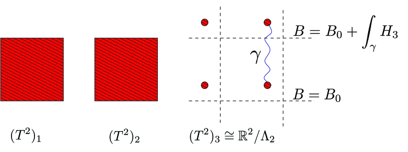
Figure 4: Open string wavefunction for a D7-brane winding mode in the T-dual type IIB flux picture. Even if both ends of the open string sit on the same point in the internal space, they feel a different B-field due to the presence of the NSNS flux $H_{3}$ and the extended nature of the winding mode. As a result, D7-brane winding modes behave as open strings that end on D7-branes with different magnetizations, and so do their wavefunctions.

Turning now to the wavefunctions for fermions and 4d scalars, it is easy to see that D7-brane KK modes should be insensitive to the presence of the flux. Winding modes, on the other hand, should feel the background flux in a more involved way than their gauge boson counterparts, as it is manifest from the matrix $\mathbb{M}$ that appears in their equation of motion in the type I picture, and which contains off diagonal terms proportional to the components of $F_{2}^{\text{cl}}$. In the case of the example (7.25) with vanishing $\mu$-terms on the D7, the off-diagonal terms should correspond to those of (4.3), and they may be understood as the mixing terms $G_{m}^{\ \,p}$ that usually appear in the equations of motion for magnetized D-branes (see e.g., eq.(2.24)), with the substitution $F_{2}\rightarrow F_{2}^{\text{cl}}$. The interpretation of these off-diagonal terms for the example with non-vanishing $\mu$-term (7.26) (given by those of (4.8)) remain however more obscure from the type IIB viewpoint. Note in particular that, according to our first dictionary above, the eigenfunctions (4.11) and (4.12) obtained in the type I side, should correspond to a bound state of winding modes of D7-brane Wilson lines and moduli. It would be interesting to understand how these eigenstates arise from the type IIB side of the duality.

Finally, let us consider those matter field wavefunctions analyzed in Section 6. From the type IIB side, the exotic W boson wavefunction (6.22) and its generalization to non-vanishing D-term should arise from a D7-brane winding mode which also feels a difference on the open string magnetic flux $\Delta F_{2}=(F_{2}^{\alpha\beta})^{\text{op}}$. Hence, in this picture the total difference in flux felt by such a D7_α-D7_β string is given by the gauge invariant quantity

$$\Delta{\cal F}\,=\,\Delta B|_{\text{D7}}+2\pi\alpha^{\prime}\Delta F_{2}\,=\,2\pi F_{2}^{\text{cl}}+2\pi(F_{2}^{\alpha\beta})^{\text{op}}\,=\,2\pi(F_{2}^{\alpha\beta})_{\text{eff}}$$ (7.29)

which is nothing but the open + closed effective flux entering the definition of the wavefunction (6.11) and the more massive modes of this sector. Hence, we find that the open string wavefunctions obtained in the type I flux vacua studied in this paper fit nicely into our understanding of the D7-brane wavefunctions physics in the type IIB T-dual setup.

8 Conclusions and outlook

In this work we have given a concrete prescription for performing dimensional reduction in flux compactifications. The procedure relies on the observation that in presence of closed string fluxes it is still possible to define some modified Dirac and Laplace-Beltrami operators in the internal manifold which account for the effect of the fluxes on the open string fluctuations. These operators are extracted from the type I supergravity action in the limit on which closed string fluctuations are frozen and the warping can be neglected.

To analyze the spectrum of eigenmodes of these operators, we have found very helpful some of the tools of non-commutative harmonic analysis and representation theory, which we have summarized in Section 3.2 and Appendix D. This formalism seems to point out towards a deep connection between the 4d spectrum of massive excitations, symplectic geometry and 4d gauged supergravity algebras. In particular, we have found that the spectrum of Kaluza-Klein excitations for neutral and charged modes in a stack of magnetized D9-branes is classified by irreducible unitary representations of the Kaloper-Myers gauge algebra [27]. Notice that for sectors of the theory which preserve enough number of supersymmetries, one can in addition consider the global symmetries of the effective action and compute other massive excitations such as winding modes. Indeed, notice that the Kaloper-Myers algebra is only a portion of the full $\mathcal{N}=4$ gauged supergravity algebra. It is therefore natural to conjecture that irreducible unitary representations of the full algebra classify not only Kaluza-Klein modes, but also winding and non-perturbative modes associated to the $\mathcal{N}=4$ sectors of the theory. Following this philosophy we have conjectured the presence of some massive non-perturbative charged modes in the worldvolume of magnetized D9-branes.

We can extract several conclusions from the results of this paper. First, notice that generically there is always a set of fields which is insensitive to the background fluxes, and therefore their wavefunctions are the same than in a fluxless compactification. Moreover, the on-shell conditions usually ensure that these are the lightest modes in the limit of diluted fluxes and constant warping, which has two important consequences. On the one side, the lightest sector is usually not affected by the fluxes, up to possible flux induced mass terms. On the other, if one considers only this sector of the theory, it is enough to dimensionally reduce as if being in a fluxless compactification.

Thus, we find that fluxes mainly affect the structure of massive Kaluza-Klein replicas. In particular, for the class of vacua that we have considered, the resulting spectrum can be understood in terms of Landau degeneracies, mass shifts and mixings induced by the fluxes. We therefore expect that fluxes change in an important way the threshold corrections to the 4d low energy effective theory. The computation of gauge threshold corrections in flux compactifications will be addressed in a future publication [28].

We have also observed that wavefunctions in the presence of closed string fluxes are not very different from wavefunctions in compactifications with only magnetized branes. This has been interpreted in the light of open/closed string duality, showing that in many cases the closed string fluxes can be interpreted as non diagonal magnetic fluxes in a dual background.

There are several possible further directions to explore, apart from the ones already mentioned. For example, it would be interesting to see how the warping fits in this picture, and in particular to try to combine these results with the ones e.g. in [39]. This is particularly important for applying these methods in the context of the AdS/CFT correspondence. Some recent applications of wavefunctions in this context include models of holographic gauge mediation [72], where Kaluza-Klein modes mediate the transmission of supersymmetry breaking between the hidden and visible sectors, and models for meson spectroscopy (see [73] for a review and references), where meson resonances are identified with Kaluza-Klein modes in a dual supergravity theory. We expect that the techniques introduced here will result useful in these contexts, once they are extended conveniently to account for the strong warping.

Also, one could similarly consider other vacua different than the no-scale solutions that we have analyzed. For instance, we could make use of the same methods for dimensionally reduce type IIA $\textrm{AdS}_{4}$ compactifications on nearly Kähler manifolds, in the same spirit than in [74, 25]. This would be particularly relevant for computing the structure of massive modes in these backgrounds.

Finally, from the phenomenological point of view, the vacua considered here are not very appealing, since they are non-chiral. In this sense, it would be desirable to extend this computation to models including magnetized D5-branes and more realistic matter content. In particular, the T-duals of the chiral flux compactifications considered in [75] fall into this class. With that same aim, it would be also desirable to extend these techniques to general, non-parallelizable SU(3)-structure manifolds.

Appendix A Fermion conventions

In order to describe explicitly fermionic wavefunctions we take the following representation for $\Gamma$-matrices in flat 10d space

$$\Gamma^{\underline{\mu}}\,=\,\gamma^{\mu}\otimes{\mathbb{I}}_{2}\otimes{\mathbb{I}}_{2}\otimes{\mathbb{I}}_{2}\quad\quad\quad\Gamma^{\underline{m}}\,=\,\gamma_{(4)}\otimes\tilde{\gamma}^{m-3}$$ (A.1)

where $\mu=0,\dots,3$, labels the 4d Minkowski coordinates, whose gamma matrices are

$$\gamma^{0}\,=\,\left(\begin{array}[]{cc}0&-{\mathbb{I}}_{2}\\ {\mathbb{I}}_{2}&0\end{array}\right)\quad\gamma^{i}\,=\,\left(\begin{array}[]{cc}0&\sigma_{i}\\ \sigma_{i}&0\end{array}\right)$$ (A.2)

$m=4,\dots,9$ labels the extra ${\cal R}^{6}$ coordinates

$$\begin{array}[]{lll}\tilde{\gamma}^{1}\,=\,\sigma_{1}\otimes{\mathbb{I}}_{2}\otimes{\mathbb{I}}_{2}&&\tilde{\gamma}^{4}\,=\,\sigma_{2}\otimes{\mathbb{I}}_{2}\otimes{\mathbb{I}}_{2}\\ \tilde{\gamma}^{2}\,=\,\sigma_{3}\otimes\sigma_{1}\otimes{\mathbb{I}}_{2}&&\tilde{\gamma}^{5}\,=\,\sigma_{3}\otimes\sigma_{2}\otimes{\mathbb{I}}_{2}\\ \tilde{\gamma}^{3}\,=\,\sigma_{3}\otimes\sigma_{3}\otimes\sigma_{1}&&\tilde{\gamma}^{6}\,=\,\sigma_{3}\otimes\sigma_{3}\otimes\sigma_{2}\end{array}$$ (A.3)

and $\sigma_{i}$ indicate the usual Pauli matrices. The 4d chirality operator is then given by

$$\Gamma_{(4)}\,=\,\gamma_{(4)}\otimes{\mathbb{I}}_{2}\otimes{\mathbb{I}}_{2}\otimes{\mathbb{I}}_{2}$$ (A.4)

where $\gamma_{(4)}=i\gamma^{0}\gamma^{1}\gamma^{2}\gamma^{3}$, and the 10d chirality operator by

$$\Gamma_{(10)}\,=\,\gamma_{(4)}\otimes\gamma_{(6)}\,=\,\left(\begin{array}[]{cc}{\mathbb{I}}_{2}&0\\ 0&-{\mathbb{I}}_{2}\end{array}\right)\otimes\sigma_{3}\otimes\sigma_{3}\otimes\sigma_{3}$$ (A.5)

with $\gamma_{(6)}=-i\tilde{\gamma}^{1}\tilde{\gamma}^{2}\tilde{\gamma}^{3}\tilde{\gamma}^{4}\tilde{\gamma}^{5}\tilde{\gamma}^{6}$. Finally, in this choice of representation a Majorana matrix is given by

$$\mathcal{B}\,=\,\Gamma^{\underline{2}}\Gamma^{\underline{7}}\Gamma^{\underline{8}}\Gamma^{\underline{9}}\,=\,\left(\begin{array}[]{cc}0&\sigma_{2}\\ -\sigma_{2}&0\end{array}\right)\otimes\sigma_{2}\otimes i\sigma_{1}\otimes\sigma_{2}\,=\,\mathcal{B}_{4}\otimes\mathcal{B}_{6}$$ (A.6)

which indeed satisfies the conditions $\mathcal{B}\mathcal{B}^{*}={\mathbb{I}}$ and $\mathcal{B}\,\Gamma^{\underline{M}}\mathcal{B}^{*}=\Gamma^{\underline{M}*}$. Notice that the 4d and 6d Majorana matrices $\mathcal{B}_{4}\equiv\gamma^{2}\gamma_{(4)}$ and $\mathcal{B}_{6}\equiv\tilde{\gamma}^{4}\tilde{\gamma}^{5}\tilde{\gamma}^{6}$ satisfy analogous conditions $\mathcal{B}_{4}\mathcal{B}_{4}^{*}=\mathcal{B}_{6}\mathcal{B}_{6}^{*}={\mathbb{I}}$ and $\mathcal{B}_{4}\,\gamma^{\mu}\mathcal{B}_{4}^{*}=\gamma^{\mu*}$, $\mathcal{B}_{6}\,\gamma^{m}\mathcal{B}_{6}^{*}=-\gamma^{m*}$.

In the text we mainly work with 10d Majorana-Weyl spinors of negative chirality, meaning those spinors $\theta$ satisfying $\theta=-\Gamma_{(10)}\theta=\mathcal{B}^{*}\theta^{*}$. In the conventions above this means that we have spinors of the form

$$\theta^{0}\,=\,\psi^{0}\,\left(\begin{array}[]{c}\xi_{+}\\ 0\end{array}\right)\otimes\chi_{---}+i(\psi^{0})^{*}\,\left(\begin{array}[]{c}0\\ \sigma_{2}\xi_{+}^{*}\end{array}\right)\otimes\chi_{+++}$$ (A.7e)

$$\theta^{1}\,=\,\psi^{1}\,\left(\begin{array}[]{c}\xi_{+}\\ 0\end{array}\right)\otimes\chi_{-++}-i(\psi^{1})^{*}\,\left(\begin{array}[]{c}0\\ \sigma_{2}\xi_{+}^{*}\end{array}\right)\otimes\chi_{+--}$$ (A.7j)

$$\theta^{2}\,=\,\psi^{2}\,\left(\begin{array}[]{c}\xi_{+}\\ 0\end{array}\right)\otimes\chi_{+-+}+i(\psi^{2})^{*}\,\left(\begin{array}[]{c}0\\ \sigma_{2}\xi_{+}^{*}\end{array}\right)\otimes\chi_{-+-}$$ (A.7o)

$$\theta^{3}\,=\,\psi^{3}\,\left(\begin{array}[]{c}\xi_{+}\\ 0\end{array}\right)\otimes\chi_{++-}-i(\psi^{3})^{*}\,\left(\begin{array}[]{c}0\\ \sigma_{2}\xi_{+}^{*}\end{array}\right)\otimes\chi_{--+}$$ (A.7t)

where $\psi^{j}$ is the spinor wavefunction, $(\xi_{+}\ 0)^{t}$ is a 4d spinor of positive chirality and $\chi_{\epsilon_{1}\epsilon_{2}\epsilon_{3}}$ is a basis of 6d spinors of such that

$$\chi_{---}\,=\,\left(\begin{array}[]{c}0\\ 1\end{array}\right)\otimes\left(\begin{array}[]{c}0\\ 1\end{array}\right)\otimes\left(\begin{array}[]{c}0\\ 1\end{array}\right)\quad\quad\chi_{+++}\,=\,\left(\begin{array}[]{c}1\\ 0\end{array}\right)\otimes\left(\begin{array}[]{c}1\\ 0\end{array}\right)\otimes\left(\begin{array}[]{c}1\\ 0\end{array}\right)$$ (A.8)

etc. Note that these basis elements are eigenstates of the 6d chirality operator $\gamma_{(6)}$, with eigenvalues $\epsilon_{1}\epsilon_{2}\epsilon_{3}$.

Finally, let us recall that to dimensionally reduce a 10d fermionic action, one has to simultaneously diagonalize two Dirac operators: $\not{\partial}_{\mathbb{R}^{1,3}}$ and $\not{D}^{\text{int}}$, built from $\Gamma^{\underline{\mu}}$ and $\Gamma^{\underline{m}}$, respectively. However, as these two set of $\Gamma$-matrices do not commute, nor will $\not{\partial}_{\mathbb{R}^{1,3}}$ and $\not{D}^{\text{int}}$, and so we need instead to construct these Dirac operators from the alternative $\Gamma$-matrices

$$\tilde{\Gamma}^{\underline{\mu}}\,=\,\Gamma_{(4)}\Gamma^{\underline{\mu}}\,=\,\Gamma_{(4)}\gamma^{\mu}\otimes{\mathbb{I}}_{2}\otimes{\mathbb{I}}_{2}\otimes{\mathbb{I}}_{2}\quad\quad\quad\tilde{\Gamma}^{\underline{m}}\,=\,\Gamma_{(4)}\Gamma^{\underline{m}}\,=\,{\mathbb{I}}_{4}\otimes\tilde{\gamma}^{m-3}$$ (A.9)

following the common practice in the literature.

Appendix B Warped Dirac equation

Let us consider the 6d Dirac equation deduced in eq.(2.25)

$$\left(\not{D}^{{\cal M}_{6}}+\frac{1}{4}e^{\phi/2}\not{F}_{3}-\frac{1}{2}\not{\partial}\ln Z\right)\chi_{6}\,=\,Z^{1/4}m_{\chi}\,\mathcal{B}_{6}^{*}\chi_{6}^{*}$$ (B.1)

where now all slashed quantities are constructed from the set of $\Gamma$-matrices defined in (A.9). Let us also consider a compactification ansatz of the form (2.28), where again $Z$ only depends on the coordinates of the base $B_{4}$.

Then, as in [11], the 2-form $J$ splits as $J=J_{\Pi_{2}}+J_{B_{4}}$, and we can split $F_{3}$ accordingly. Indeed, let us define

$$e^{\phi/2}F_{3}^{\rm bg}\,\equiv\,e^{\phi/2}F_{3}-2*_{{\cal M}_{6}}(d\phi\wedge J_{\Pi_{2}})$$ (B.2)

so that eq.(B.1) becomes

$$\left(\not{D}^{{\cal M}_{6}}+\frac{1}{4}e^{\phi/2}\not{F}_{3}^{\rm bg}-\not{\partial}\ln Z\,P_{+}^{\Pi_{2}}\right)\chi_{6}\,=\,Z^{-1/4}m_{4}\,{\cal B}_{6}^{*}\chi_{6}^{*}$$ (B.3)

where we have introduced the projectors $P_{\pm}^{\Pi_{2}}$ defined in (2.30). In addition, we have that the covariant derivative reads

$$\nabla^{{\cal M}_{6}}_{m}\,=\,\partial_{m}+\omega^{B_{4}}_{m}-\frac{1}{8}\left(\partial_{m}\ln Z-\Gamma_{m}\not{\partial}\ln Z\right)-\frac{1}{4}\Lambda_{m}{}^{n}\left(\partial_{n}\ln Z-\Gamma_{n}\not{\partial}\ln Z-\not{f}_{n}\right)$$ (B.4)

where $\omega^{B_{4}}$ is the spin connection of $B_{4}$, $f_{mnp}$ is defined by (2.32) and $\Lambda$ is a block-diagonal matrix specified by

$$\Lambda_{mn}\,=\,g_{mn}-2e^{{a}}_{m}e_{{a}n},\quad\quad a\in\Pi_{2}$$ (B.5)

Finally, (B.2) implies that

$$e^{\phi/2}F_{3}^{\rm bg}\,=\,*_{{\cal M}_{6}}\left[e^{\phi/2}d\left(e^{-\phi/2}J_{\Pi_{2}}\right)+e^{-3\phi/2}d\left(e^{3\phi/2}J_{B_{4}}\right)\right]$$ (B.6)

and this, if the $B_{4}$ base is symplectic, implies that $e^{\phi/2}\not{F}_{3}^{\text{bg}}=i\not{f}\not{J}_{\Pi_{2}}\gamma_{(6)}$.

We thus obtain a 6d Dirac equation of the form

$$\left(\not{D}^{\Pi_{2}}+\not{D}^{B_{4}}+\frac{1}{2}\not{f}P_{+}^{\Pi_{2}}-\not{\partial}\ln Z\left(P_{+}^{\Pi_{2}}-\frac{7}{8}\right)\right)\chi_{6}\,=\,Z^{1/4}m_{4}\,{\cal B}_{6}^{*}\chi_{6}^{*}$$ (B.7)

containing the coupling of fermions to the warping. Note that by taking $Z=1$ we recover the unwarped equation (2.31) used in the main text.

Now, if we normalize the internal spinor as $\chi_{6}^{\dagger}\chi_{6}=1$, then the warp factor dependence of the metric ansatz (2.28) will induce a non-standard 4d kinetic terms for $\chi_{4}$. In order to recover a canonical kinetic terms upon dimensional reduction we need instead to consider the rescaled Weyl fermion

$$\eta\,\equiv\,Z^{-7/8}\,\chi_{6}$$ (B.8)

in terms of which the warped 6d Dirac equation reads

$$\left(\not{D}^{\Pi_{2}}+\not{D}^{B_{4}}+\frac{1}{2}\not{f}P_{+}^{\Pi_{2}}-\not{\partial}\ln ZP_{+}^{\Pi_{2}}\right)\eta\,=\,Z^{1/4}m_{4}\,{\cal B}_{6}^{*}\eta^{*}$$ (B.9)

Note that the projector $P_{+}^{\Pi_{2}}$ is basically the chirality projector of the 4d base $B_{4}$. As in (2.33), let us split $\eta$ as

$$\eta\,=\,\eta_{\Pi_{2}}+\eta_{B_{4}}$$ (B.10)

where $P_{+}^{\Pi_{2}}\eta_{\Pi_{2}}=\eta_{\Pi_{2}}$, $P_{+}^{\Pi_{2}}\eta_{B_{4}}=0$. We can then split the Dirac equation (B.9) as

$${\not{D}}^{\Pi_{2}}_{\text{uw}}\eta_{B_{4}}+{\not{D}}^{B_{4}}_{\text{uw}}Z^{-1}\eta_{\Pi_{2}} = m_{4}{\cal B}_{6}^{*}\eta_{B_{4}}^{*}$$ (B.11)

$${\not{D}}^{\Pi_{2}}_{\text{uw}}\eta_{\Pi_{2}}+Z^{-1}{\not{D}}^{B_{4}}_{\text{uw}}\eta_{B_{4}}+\frac{1}{2}Z^{-2}{\not{f}}_{\text{uw}}\eta_{\Pi_{2}} = m_{4}{\cal B}_{6}^{*}\eta_{\Pi_{2}}^{*}$$ (B.12)

where we have extracted the warp factor dependence from the $\Gamma$-matrices contractions.

Note that a simple set of solutions is obtained by setting $\eta_{\Pi_{2}}=0$, $m_{4}=0$ and $\not{D}^{B_{4}}\eta_{B_{4}}=0$, since neither the warp factor nor the fluxes play any role in this case. This simple zero mode equation does not come as a surprise if one compares eq.(B.9) with the Dirac equation for D7-branes in type IIB warped Calabi-Yau flux backgrounds. Indeed, by the results of [39] it is easy to identify the modes $\eta_{\Pi_{2}}$ in (B.10) as those containing the gaugino and geometric modulini of a T-dual D7-brane, as well as their KK replicas, whereas $\eta_{B_{4}}$ are T-dual to the D7-brane Wilsonini. Now, since the Wilson line zero modes of a D7-brane do not feel the effect of the background fluxes [9, 70] nor that of the warping [39], the same statement must apply to the open string zero modes arising from $\eta_{B_{4}}$, as is indeed the case.

Appendix C A non-supersymmetric example

On the main text we have analyzed examples where the closed string background fluxes preserve at least $\mathcal{N}=1$ supersymmetry in four dimensions. However, as we have treated bosons and fermions independently, our techniques apply equally well to ${{\cal N}=0}$ vacua of the theory. To illustrate this fact, in this appendix we apply them to one of such examples, based on a compactification on the Heisenberg manifold.

Let us then consider the background

$$ds^{2}=Z^{-1/2}(ds^{2}_{\mathbb{R}^{1,3}}+ds^{2}_{\Pi_{2}})+Z^{3/2}ds^{2}_{T^{4}}$$ (C.1a)

$$ds^{2}_{T^{4}}=(2\pi)^{2}\sum_{m=1,2,4,5}(R_{m}dx^{m})^{2}$$ (C.1b)

$$ds^{2}_{\Pi_{2}}=(2\pi)^{2}[(R_{3}dx^{3})^{2}+(R_{6}\tilde{e}^{6})^{2}]$$ (C.1c)

$$F_{3}=-(2\pi)^{2}Ndx^{1}\wedge dx^{2}\wedge\tilde{e}^{6}-g_{s}^{-1}*_{T^{4}}dZ^{2}$$ (C.1d)

$$e^{\phi}Z=g_{s}=\textrm{const.}$$ (C.1e)

which is almost identical to (2.46). In the present case, however, $\tilde{e}^{6}$ stands for the left-invariant 1-form satisfying

$$d\tilde{e}^{6}=Mdx^{4}\wedge dx^{5}$$ (C.2)

so that $\mathcal{M}_{6}$ is given locally by $\mathbb{R}\times\mathcal{H}_{3}$. The twisted derivatives are then

$$\hat{\partial}_{1} =(2\pi R_{1})^{-1}\partial_{x^{1}} \hat{\partial}_{4} =(2\pi R_{4})^{-1}(\partial_{x^{4}}+\frac{M}{2}x^{5}\partial_{x^{6}})$$

$$\hat{\partial}_{2} =(2\pi R_{2})^{-1}\partial_{x^{2}} \hat{\partial}_{5} =(2\pi R_{5})^{-1}(\partial_{x^{5}}-\frac{M}{2}x^{4}\partial_{x^{6}})$$

$$\hat{\partial}_{3} =(2\pi R_{3})^{-1}\partial_{x^{3}} \hat{\partial}_{6} =(2\pi R_{6})^{-1}\partial_{x^{6}}$$

Finally, the compact structure of $\mathcal{M}_{6}$ is produced by the following identifications which result from quotienting by $\Gamma=\Gamma_{{\cal H}_{3}}\times\mathbb{Z}^{3}$

$$x^{4}\to x^{4}+1\qquad x^{6}\to x^{6}-\frac{M}{2}x^{5}$$

$$x^{5}\to x^{5}+1\qquad x^{6}\to x^{6}+\frac{M}{2}x^{4}$$

$$x^{i}\to x^{i}+1\qquad\qquad\textrm{for }i\neq 4,5$$

In addition, the equations of motion require the conditions $R_{4}R_{5}=4\pi^{2}R_{6}^{2}R_{1}R_{2}$ and $g_{s}N=M$, with $N,\ M\in\mathbb{Z}$. This in particular ensures that the first torsion class $\mathcal{W}_{1}$, defined as $J\wedge d\Omega=\mathcal{W}_{1}J\wedge J\wedge J$, is non-vanishing and, hence, $\mathcal{M}_{6}$ is not a complex manifold. As the gravitino mass is proportional to $\mathcal{W}_{1}$ [11, 65, 35], this reflects the fact that the background does not preserves any supersymmetry in 4d.

As in our previous examples, in order to cancel the RR charges and tensions, O5-planes (and maybe also D5-branes) wrapping $\Pi_{2}$ are required, which again will be introduced via the orbifold quotient $\mathcal{R}:x^{m}\mapsto-x^{m}$ on the $T^{4}$ base coordinates. To simplify our discussion, in this section we will assume $F_{2}=0$, although one can easily add the effect of a non-trivial $F_{2}$ along the lines of Section 6.

C.1 Bosonic wavefunctions

As usual, the wavefunction for the four dimensional neutral gauge bosons is given by the eigenfunctions of the corresponding Laplace-Beltrami operator of the manifold

$$\hat{\partial}_{m}\hat{\partial}^{m}B=-m_{B}^{2}B$$ (C.3)

The solutions to this equations can be found using the techniques described in Section 3. More precisely, we find two towers of KK modes associated to the four dimensional gauge boson, which in a suitable polarization read

$$B_{k_{1},k_{2},k_{3},k_{4},k_{5}}(\vec{x})=\textrm{exp}[2\pi i(k_{1}x^{1}+k_{2}x^{2}+k_{3}x^{3}+k_{4}x^{4}+k_{5}x^{5})]$$ (C.4)

for the first tower, with mass eigenvalue

$$m_{B}^{2}=\sum_{i=1}^{5}\left(\frac{k_{i}}{R_{i}}\right)^{2}$$ (C.5)

while for the second tower

$$B^{\delta}_{n,k_{1},k_{2},k_{3},k_{6}}=\left(\frac{2\pi^{2}R_{5}|k_{6}M|}{R_{4}\textrm{Vol}_{\mathcal{M}_{6}}}\right)^{1/4}\sum_{k_{4}\in\delta+k_{6}M\mathbb{N}}\psi_{n}\left(\frac{\dot{x}^{5}}{\sqrt{2}}\right)e^{2\pi i\left(k_{1}x^{1}+k_{2}x^{2}+k_{3}x^{3}+k_{4}x^{4}+k_{6}\dot{x}^{6}\right)}$$ (C.6)

with eigenvalue

$$m_{B}^{2}=\frac{|k_{6}\varepsilon|}{R_{6}}(2n+1)+\sum_{m=1,2,3,6}\left(\frac{k_{m}}{R_{m}}\right)^{2}$$ (C.7)

with $\delta=0\ldots k_{6}M-1$, $\varepsilon=MR_{6}/2\pi R_{4}R_{5}$ and

$$\dot{x}^{5}=\left(\frac{4\pi R_{5}}{R_{4}|k_{6}M|}\right)^{1/2}(k_{4}+k_{6}M)\quad\qquad\dot{x}^{6}\equiv x^{6}+\frac{M}{2}x^{4}x^{5}$$ (C.8)

Similarly, we can work out the wavefunctions for the four dimensional scalars. Plugging the background into eqs.(2.36)-(2.37) leads to an equation of the form (4.1) where, in complex coordinates (4.2), the mass matrix now reads

$$\mathbb{M}=\begin{pmatrix}\hat{\partial}_{m}\hat{\partial}^{m}&-\varepsilon\hat{\partial}_{6}&-\frac{i\varepsilon}{2}\hat{\partial}_{z^{2}}&0&0&\frac{i\varepsilon}{2}\hat{\partial}_{z^{2}}\\ \varepsilon\hat{\partial}_{6}&\hat{\partial}_{m}\hat{\partial}^{m}&\frac{i\varepsilon}{2}\hat{\partial}_{z^{1}}&0&0&-\frac{i\varepsilon}{2}\hat{\partial}_{z^{1}}\\ -\frac{i\varepsilon}{2}\hat{\partial}_{\bar{z}^{2}}&\frac{i\varepsilon}{2}\hat{\partial}_{\bar{z}^{1}}&\hat{\partial}_{m}\hat{\partial}^{m}-\frac{\varepsilon^{2}}{2}&-\frac{i\varepsilon}{2}\hat{\partial}_{z^{2}}&\frac{i\varepsilon}{2}\hat{\partial}_{z^{1}}&\frac{\varepsilon^{2}}{2}\\ 0&0&-\frac{i\varepsilon}{2}\hat{\partial}_{\bar{z}^{2}}&\hat{\partial}_{m}\hat{\partial}^{m}&-\varepsilon\hat{\partial}_{6}&\frac{i\varepsilon}{2}\hat{\partial}_{\bar{z}^{2}}\\ 0&0&\frac{i\varepsilon}{2}\hat{\partial}_{\bar{z}^{1}}&\varepsilon\hat{\partial}_{6}&\hat{\partial}_{m}\hat{\partial}^{m}&-\frac{i\varepsilon}{2}\hat{\partial}_{\bar{z}^{1}}\\ \frac{i\varepsilon}{2}\hat{\partial}_{\bar{z}^{2}}&-\frac{i\varepsilon}{2}\hat{\partial}_{\bar{z}^{1}}&\frac{\varepsilon^{2}}{2}&\frac{i\varepsilon}{2}\hat{\partial}_{z^{2}}&-\frac{i\varepsilon}{2}\hat{\partial}_{z^{1}}&\hat{\partial}_{m}\hat{\partial}^{m}-\frac{\varepsilon^{2}}{2}\end{pmatrix}$$ (C.9)

This is a non-commutative eigenvalue problem similar to the one found in Section 4.2. Notice, however, that in the present case the mass matrix is not block diagonal, reflecting the fact that the background does not preserves the complex structure of $T^{6}$, and in particular the complex structure given by the choice (4.2).

As in the supersymmetric case, the eigenvalues and eigenfunctions of (C.9) can be found we the aid of the commutation relations of the twisted derivatives and the Laplacian, which in the present case read

$$[\hat{\partial}_{{z}^{1}},\hat{\partial}_{{z}^{2}}]\,=\,[\hat{\partial}_{\bar{z}^{1}},\hat{\partial}_{\bar{z}^{2}}]\,=\,\varepsilon\hat{\partial}_{6}\quad\quad[\hat{\partial}_{{z}^{1}},\hat{\partial}_{\bar{z}^{2}}]\,=\,[\hat{\partial}_{\bar{z}^{1}},\hat{\partial}_{{z}^{2}}]\,=\,-\varepsilon\hat{\partial}_{6}$$

$$-[\hat{\partial}_{m}\hat{\partial}^{m},\hat{\partial}_{{z}^{1}}]\,=\,[\hat{\partial}_{m}\hat{\partial}^{m},\hat{\partial}_{\bar{z}^{1}}]\,=\,\varepsilon\hat{\partial}_{6}(\hat{\partial}_{\bar{z}^{2}}-\hat{\partial}_{z^{2}})$$

$$[\hat{\partial}_{m}\hat{\partial}^{m},\hat{\partial}_{{z}^{2}}]\,=\,-[\hat{\partial}_{m}\hat{\partial}^{m},\hat{\partial}_{\bar{z}^{2}}]\,=\,\varepsilon\hat{\partial}_{6}(\hat{\partial}_{\bar{z}^{1}}-\hat{\partial}_{z^{1}})$$

After some work, we find that the resulting spectrum is given by the two eigenvectors

$$\xi_{3}(\vec{x})\equiv\begin{pmatrix}0\\ 0\\ 1\\ 0\\ 0\\ 1\end{pmatrix}B(\vec{x})\quad\qquad\xi_{3}^{*}(\vec{x})\equiv\begin{pmatrix}\hat{\partial}_{\bar{z}^{1}}\\ \hat{\partial}_{\bar{z}^{2}}\\ 2i\hat{\partial}_{6}\\ \hat{\partial}_{{z}^{1}}\\ \hat{\partial}_{{z}^{2}}\\ 0\end{pmatrix}B(\vec{x})$$ (C.10)

with mass eigenvalues $m_{\xi_{3}}^{2}=m_{\xi_{3}^{*}}^{2}=m_{B}^{2}$, the two eigenvectors

$$\xi_{+}(\vec{x})\equiv\begin{pmatrix}\hat{\partial}_{\bar{z}^{1}}-i\hat{\partial}_{{z}^{2}}\\ \hat{\partial}_{\bar{z}^{2}}+i\hat{\partial}_{{z}^{1}}\\ 0\\ -\hat{\partial}_{{z}^{1}}+i\hat{\partial}_{\bar{z}^{2}}\\ -\hat{\partial}_{{z}^{2}}-i\hat{\partial}_{\bar{z}^{1}}\\ 0\end{pmatrix}(\hat{\partial}_{4}-i\hat{\partial}_{5})B(\vec{x})\quad\qquad\xi_{-}(\vec{x})\equiv\begin{pmatrix}-\hat{\partial}_{\bar{z}^{1}}-i\hat{\partial}_{{z}^{2}}\\ -\hat{\partial}_{\bar{z}^{2}}+i\hat{\partial}_{{z}^{1}}\\ 0\\ \hat{\partial}_{{z}^{1}}+i\hat{\partial}_{\bar{z}^{2}}\\ \hat{\partial}_{{z}^{2}}-i\hat{\partial}_{\bar{z}^{1}}\\ 0\end{pmatrix}(\hat{\partial}_{4}+i\hat{\partial}_{5})B(\vec{x})$$ (C.11)

with mass eigenvalues $m_{\xi_{\pm}}^{2}=m_{B}^{2}\pm(\varepsilon k_{6}/R_{6})$, and the two eigenvectors

$$\xi_{\pm}^{*}\equiv\begin{pmatrix}-(m^{2}_{\xi_{\pm}^{*}}-m^{2}_{B})\hat{\partial}_{z^{2}}+\varepsilon\hat{\partial}_{\bar{z}^{1}}\hat{\partial}_{6}\\ (m^{2}_{\xi_{\pm}^{*}}-m^{2}_{B})\hat{\partial}_{z^{1}}+\varepsilon\hat{\partial}_{\bar{z}^{2}}\hat{\partial}_{6}\\ i\frac{(m^{2}_{\xi_{\pm}^{*}}-m^{2}_{B})^{2}}{\varepsilon}+i\varepsilon\hat{\partial}_{6}\\ -(m^{2}_{\xi_{\pm}^{*}}-m^{2}_{B})\hat{\partial}_{\bar{z}^{2}}+\varepsilon\hat{\partial}_{{z}^{1}}\hat{\partial}_{6}\\ (m^{2}_{\xi_{\pm}^{*}}-m^{2}_{B})\hat{\partial}_{\bar{z}^{1}}+\varepsilon\hat{\partial}_{{z}^{2}}\hat{\partial}_{6}\\ -i\frac{(m^{2}_{\xi_{\pm}^{*}}-m^{2}_{B})^{2}}{\mu}+i\varepsilon\hat{\partial}_{6}\end{pmatrix}B(\vec{x})$$ (C.12)

with mass eigenvalue

$$m^{2}_{\xi_{\pm}^{*}}=\frac{1}{4}\left(\varepsilon\pm\sqrt{\varepsilon^{2}+4m_{B}^{2}-4\left(\frac{k_{3}}{R_{3}}\right)^{2}}\right)^{2}+\left(\frac{k_{3}}{R_{3}}\right)^{2}$$ (C.13)

where in all these expressions $B(\vec{x})$ is a gauge boson wavefunction, (C.4)-(C.6), with mass eigenvalue $m_{B}$.

C.2 Fermionic wavefunctions

Regarding the fermionic wavefunctions, in this case we have that

$$\not{f}\,=\,(2\pi)^{-1}\frac{MR_{6}}{R_{4}R_{5}}\tilde{\gamma}^{456}\,=\,(2\pi)^{-1}\frac{MR_{6}}{R_{4}R_{5}}\,i\sigma_{2}\otimes\sigma_{1}\otimes\sigma_{2}\,=\,\varepsilon{\cal B}_{6}$$ (C.14)

and so the Dirac operator reads

$${\bf D}+{\bf F}\,=\,\left(\begin{array}[]{cccc}i\frac{\varepsilon}{2}&\hat{\partial}_{{z}^{1}}&\hat{\partial}_{{z}^{2}}&\hat{\partial}_{{z}^{3}}\\ -\hat{\partial}_{{z}^{1}}&0&-\hat{\partial}_{\bar{z}^{3}}&\hat{\partial}_{\bar{z}^{2}}\\ -\hat{\partial}_{{z}^{2}}&\hat{\partial}_{\bar{z}^{3}}&0&-\hat{\partial}_{\bar{z}^{1}}\\ -\hat{\partial}_{{z}^{3}}&-\hat{\partial}_{\bar{z}^{2}}&\hat{\partial}_{\bar{z}^{1}}&i\frac{\varepsilon}{2}\end{array}\right)$$ (C.15)

from which we extract the following mass matrix

$$-({\bf D}+{\bf F})^{*}({\bf D}+{\bf F})\,=\,\left(\begin{array}[]{cccc}\hat{\partial}_{m}\hat{\partial}^{m}-\frac{\varepsilon^{2}}{4}&i\frac{\varepsilon}{2}\hat{\partial}_{{z}^{1}}&i\frac{\varepsilon}{2}\hat{\partial}_{{z}^{2}}&0\\ i\frac{\varepsilon}{2}\hat{\partial}_{\bar{z}^{1}}&\hat{\partial}_{m}\hat{\partial}^{m}&-\varepsilon\hat{\partial}_{6}&-i\frac{\varepsilon}{2}\hat{\partial}_{{z}^{2}}\\ i\frac{\varepsilon}{2}\hat{\partial}_{\bar{z}^{2}}&\varepsilon\hat{\partial}_{6}&\hat{\partial}_{m}\hat{\partial}^{m}&i\frac{\varepsilon}{2}\hat{\partial}_{{z}^{1}}\\ 0&-i\frac{\varepsilon}{2}\hat{\partial}_{z^{2}}&i\frac{\varepsilon}{2}\hat{\partial}_{z^{1}}&\hat{\partial}_{m}\hat{\partial}^{m}-\frac{\varepsilon^{2}}{4}\end{array}\right)$$ (C.16)

Since the background does not preserve any supersymmetry, it is natural to expect the eigenfunctions and eigenvalues of this matrix to be rather different from their bosonic counterparts. Indeed, after some algebra one can show that the fermionic wavefunctions are given by the eigenvectors

$$\Psi_{\pm}(\vec{x})\equiv\begin{pmatrix}i\varepsilon(m^{2}_{\Psi_{\pm}}+\hat{\partial}_{z^{3}}\hat{\partial}_{\bar{z}^{3}})\\ 2(\hat{\partial}_{\bar{z}^{1}}+i\hat{\partial}_{z^{2}})(m^{2}_{\Psi_{\pm}}-m_{B}^{2})\\ 2(\hat{\partial}_{\bar{z}^{2}}-i\hat{\partial}_{z^{1}})(m^{2}_{\Psi_{\pm}}-m_{B}^{2})\\ \varepsilon(m^{2}_{\Psi_{\pm}}+\hat{\partial}_{z^{3}}\hat{\partial}_{\bar{z}^{3}})\end{pmatrix}B(\vec{x})\quad\qquad\Psi^{\prime}_{\pm}(\vec{x})\equiv\begin{pmatrix}-i\varepsilon(m^{2}_{\Psi^{\prime}_{\pm}}+\hat{\partial}_{z^{3}}\hat{\partial}_{\bar{z}^{3}})\\ -2(\hat{\partial}_{\bar{z}^{1}}-i\hat{\partial}_{z^{2}})(m^{2}_{\Psi^{\prime}_{\pm}}-m_{B}^{2})\\ -2(\hat{\partial}_{\bar{z}^{2}}+i\hat{\partial}_{z^{1}})(m^{2}_{\Psi^{\prime}_{\pm}}-m_{B}^{2})\\ \varepsilon(m^{2}_{\Psi^{\prime}_{\pm}}+\hat{\partial}_{z^{3}}\hat{\partial}_{\bar{z}^{3}})\end{pmatrix}B(\vec{x})$$ (C.17)

with mass eigenvalues

$$m^{2}_{\Psi_{\pm}} =\frac{1}{16}\left(\varepsilon\pm\sqrt{16m_{B}^{2}+\varepsilon^{2}-16\left(\frac{k_{3}}{R_{3}}\right)^{2}-\frac{\varepsilon k_{6}}{2R_{6}}}\right)^{2}+\left(\frac{k_{3}}{R_{3}}\right)^{2}$$ (C.18)

$$m^{2}_{\Psi^{\prime}_{\pm}} =\frac{1}{16}\left(\varepsilon\pm\sqrt{16m_{B}^{2}+\varepsilon^{2}-16\left(\frac{k_{3}}{R_{3}}\right)^{2}+\frac{\varepsilon k_{6}}{2R_{6}}}\right)^{2}+\left(\frac{k_{3}}{R_{3}}\right)^{2}$$ (C.19)

Appendix D The orbit method

In this appendix we summarize the notions of representation theory required for solving the generalized Dirac and Laplace equations in parallelizable manifolds. More precisely we consider the orbit method developed mostly by A. Kirillov in the 60’s, applied to nilmanifolds. Basically, the method relies the existence of a connection between harmonic analysis and symplectic geometry. The main objects are the orbits of a coadjoint action, which we will define in brief. These orbits turn out to be in one to one correspondence with the irreducible unitary representations of the group.

More precisely, consider a compact nilmanifold given by $\mathcal{M}=G/\Gamma$, with $G$ a nilpotent group and $\Gamma$ a discrete subgroup. For matrix groups, we can introduce the hermitian product

$$\langle A,B\rangle\equiv\textrm{Tr}(AB)$$ (D.1)

for $A,B\in\textrm{Mat}_{n}(\mathbb{R})$. We can then introduce the algebra $\mathfrak{g}^{*}$, dual to the Lie algebra of $G$, $\mathfrak{g}=\textrm{Lie}(G)$, through the partition

$$\textrm{Mat}_{n}(\mathbb{R})=\mathfrak{g}^{*}\ \oplus\ \mathfrak{g}^{\perp}$$ (D.2)

where

$$\mathfrak{g}^{\perp}=\{A\in\textrm{Mat}_{n}(\mathbb{R})\ |\ \langle A,B\rangle=0\ \forall\ B\in\mathfrak{g}\}$$ (D.3)

The coadjoint representation $K$ of $\mathfrak{g}^{*}$ is then defined as

$$K(g):\ \mathfrak{g}^{*}\to\mathfrak{g}^{*},\qquad K(g)F=p_{\mathfrak{g}^{*}}(gFg^{-1})$$ (D.4)

for $g\in G$ and $p_{\mathfrak{g}^{*}}$ the projector of $\textrm{Mat}_{n}(\mathbb{R})$ onto $\mathfrak{g}^{*}$.

The central idea underlying the orbit method then states that there is a one to one correspondence between the orbits $\Omega$ of the coadjoint action $K$, and the irreducible unitary representations of $\mathfrak{g}$ acting on $L^{2}(\mathbb{R}^{\frac{\textrm{dim }\Omega}{2}})$, given by

$$\pi_{\Omega}(g)u(\vec{s})=e^{2\pi i\langle F,\textrm{log }h(\vec{s},g)\rangle}u(\vec{s}\cdot g)$$ (D.5)

acting on $L^{2}(\mathbb{R}^{\frac{\textrm{dim }\Omega}{2}})$. This equation needs some explanation. Here, $F$ is an arbitrary point in $\Omega$, whereas $\textrm{log }h(\vec{s},g)$ represents the Lie algebra element corresponding to the group element $h(\vec{s},g)$. The latter is a solution of the master equation

$$S(\vec{s})g=h(\vec{s},g)S(\vec{s}\cdot g)$$ (D.6)

with $S$ a section $G/H\to G$, and $H\in G$ the subgroup corresponding to a subalgebra $\mathfrak{h}\in\mathfrak{g}$ of dimension dim $\mathfrak{h}=\textrm{dim }\mathfrak{g}-\frac{1}{2}\textrm{dim }\Omega$  such that

$$\langle F,[\mathfrak{h},\mathfrak{h}]\rangle=0$$ (D.7)

Each subalgebra of the right dimension satisfying this equation leads to a different manifold polarization of the representation associated to an orbit $\Omega$, and different polarizations are related among themselves by generalizations of the Abelian Fourier transform.

In order to illustrate this powerful procedure, in what follows we consider a couple of examples relevant for the material presented in the main text.

Example 1. Irreducible unitary representations of $\mathcal{H}_{2p+1}$

Consider the $2p+1$ dimensional Heisenberg group. As already mentioned in Section 3.1, a suitable matrix representation for the group is given by (2.44)

$$G=\begin{pmatrix}1&-\frac{1}{2}\vec{y}^{t}&\frac{1}{2}\vec{x}^{t}&z\\ 0&1&0&\vec{x}\\ 0&0&1&\vec{y}\\ 0&0&0&1\end{pmatrix}$$ (D.8)

From here the matrix representations for $\mathfrak{g}$ and $\mathfrak{g}^{*}$ are easily worked out

$${g}=\begin{pmatrix}0&-\frac{1}{2}\vec{y}^{t}&\frac{1}{2}\vec{x}^{t}&z\\ 0&0&0&\vec{x}\\ 0&0&0&\vec{y}\\ 0&0&0&0\end{pmatrix}\quad\qquad{g}^{*}=\begin{pmatrix}0&0&0&0\\ -\vec{g}_{y}&0&0&0\\ \vec{g}_{x}&0&0&0\\ g_{z}&\frac{1}{2}\vec{g}_{x}^{t}&\frac{1}{2}\vec{g}_{y}^{t}&0\end{pmatrix}$$ (D.9)

where $\vec{g}_{x}$ and $\vec{g}_{y}$ are $p$-dimensional vectors. The coadjoint representation then reads

$$K(G)(\vec{g}_{x},\vec{g}_{y},g_{z})=(\vec{g}_{x}+\vec{y}\cdot\vec{g}_{z},\ \vec{g}_{y}-\vec{x}\cdot\vec{g}_{z},\ g_{z})$$ (D.10)

Observe that there are only two types of orbits: zero dimensional orbits given by the points $\Omega_{\mu,\nu}\equiv(\vec{\mu},\vec{\nu},0)$ with $\vec{\mu}$ and $\vec{\nu}$ constant vectors, and two dimensional orbits given by the hyperplanes $\Omega_{\lambda}\equiv(*,*,\lambda)$, with $\lambda\neq 0$.

The irreducible unitary representations associated to zero dimensional orbits, $\Omega_{\mu,\nu}$, can be worked out very easily. The corresponding subalgebra is $(2p+1)$-dimensional, and therefore it is the full Heisenberg algebra. The master equation becomes trivial, and the corresponding irreducible unitary representations are given by

$$\pi_{\mu,\nu}=e^{2\pi i\langle\left.\mathfrak{g}^{*}\right|_{\Omega_{\mu,\nu}},\mathfrak{g}\rangle}=e^{2\pi i(\vec{\mu}\cdot\vec{x}+\vec{\nu}\cdot\vec{y})}$$ (D.11)

For the irreducible unitary representations associated to the $2p$-dimensional orbits, $\Omega_{\lambda}$, we have to select a $p+1$-dimensional subalgebra $\mathfrak{h}$ such that

$$\langle\left.\mathfrak{g}^{*}\right|_{\Omega_{\lambda}},\ [\mathfrak{h},\mathfrak{h}]\rangle=0$$ (D.12)

Different choices correspond to different manifold polarizations. Here, for concreteness, we focus in the subalgebra generated by $\vec{x}=0$ in (D.9). A suitable section in $G/H$ is then given by

$$S(\vec{s})=\begin{pmatrix}1&0&-\frac{1}{2}\vec{s}^{t}&0\\ 0&1&0&\vec{s}\\ 0&0&1&0\\ 0&0&0&1\end{pmatrix}$$ (D.13)

and the solution to the master equation reads

$$h(\vec{s},g)=\begin{pmatrix}1&-\frac{1}{2}\vec{y}&0&z+\frac{1}{2}\vec{s}\cdot\vec{y}\\ 0&1&0&0\\ 0&0&1&\vec{y}\\ 0&0&0&1\end{pmatrix}\qquad\vec{s}\cdot g=(\vec{x}+\vec{s},\vec{y},z)$$ (D.14)

Plugging into eq.(D.5) we finally get the irreducible unitary representations associated to the orbits $\Omega_{\lambda}$

$$\pi_{\lambda}u(\vec{s})=e^{2\pi i\lambda[z+\vec{y}\cdot\vec{s}+\vec{x}\cdot\vec{y}/2]}u(\vec{x}+\vec{s})$$ (D.15)

In this way we have rederived the Stone - von Neumann theorem, discussed in eqs.(3.38)-(3.39), by means of the orbit method. Let us now consider a more involved example.

Example 2. Irreducible unitary representations of the algebra (2.55)

Consider the nilpotent group associated to the nilmanifold defined by eq.(2.55). Matrix representations for the group, the algebra, and the dual algebra, can be easily worked out, resulting in

$$G=\begin{pmatrix}1&-\frac{M_{6}x^{1}}{2}&0&0&0&\frac{M_{6}x^{5}}{2}&x^{6}\\ 0&1&0&0&0&0&x^{5}\\ 0&0&1&0&0&0&x^{4}\\ 0&0&0&1&-\frac{M_{3}x^{1}}{2}&\frac{M_{3}x^{2}}{2}&x^{3}\\ 0&0&0&0&1&0&x^{2}\\ 0&0&0&0&0&1&x^{1}\\ 0&0&0&0&0&0&1\end{pmatrix}$$

$$\mathfrak{g}=\begin{pmatrix}0&-\frac{M_{6}x^{1}}{2}&0&0&0&\frac{M_{6}x^{5}}{2}&x^{6}\\ 0&0&0&0&0&0&x^{5}\\ 0&0&0&0&0&0&x^{4}\\ 0&0&0&0&-\frac{M_{3}x^{1}}{2}&\frac{M_{3}x^{2}}{2}&x^{3}\\ 0&0&0&0&0&0&x^{2}\\ 0&0&0&0&0&0&x^{1}\\ 0&0&0&0&0&0&0\end{pmatrix}\quad\quad\mathfrak{g}^{*}=\begin{pmatrix}0&0&0&0&0&0&0\\ -\frac{2g_{1}}{M_{6}}&0&0&0&0&0&0\\ 0&0&0&0&0&0&0\\ 0&0&0&0&0&0&0\\ 0&0&0&0&0&0&0\\ \frac{2g_{5}}{M_{6}}&0&0&\frac{2g_{2}}{M_{3}}&0&0&0\\ g_{6}&g_{5}&g_{4}&g_{3}&g_{2}&g_{1}&0\end{pmatrix}$$

The projector into $\mathfrak{g}^{*}$ is given by

$$P_{\mathfrak{g}^{*}}(A)=\begin{pmatrix}0&0&0&0&0&0&0\\ \frac{A_{21}}{2}-\frac{A_{76}}{M_{6}}&0&0&0&0&0&0\\ 0&0&0&0&0&0&0\\ 0&0&0&0&0&0&0\\ 0&0&0&0&0&0&0\\ \frac{A_{61}}{2}+\frac{A_{72}}{M_{6}}&0&0&\frac{A_{64}}{2}+\frac{A_{75}}{M_{3}}&0&0&0\\ A_{71}&\frac{A_{72}}{2}+\frac{M_{6}A_{61}}{4}&A_{73}&A_{74}&\frac{A_{75}}{2}+\frac{M_{3}A_{64}}{4}&\frac{A_{76}}{2}-\frac{M_{6}A_{21}}{4}&0\end{pmatrix}$$

From these expressions, the coadjoint representation reads

$$K(G)(g_{1},g_{2},g_{3},g_{4},g_{5},g_{6})=\left(g_{1}-\frac{1}{4}g_{3}M_{3}x^{2}-\frac{1}{2}g_{6}M_{6}x^{5},\ g_{2}+\frac{1}{2}M_{3}g_{3}x^{1},\ g_{3},\right.\\ \left.g_{4},\ g_{5}+\frac{1}{2}M_{6}g_{6}x^{1},\ g_{6}\right)$$

We observe, therefore, four classes of orbits, one 0-dimensional, and three 2-dimensional, given by

$$\Omega_{\mu,\nu,\sigma,\rho} =(\mu,\nu,0,\sigma,\rho,0)$$ (D.16)

$$\Omega_{\mu,r,p} =(*_{1},M_{3}r*_{2},r,\mu,M_{6}p*_{2},p)$$ (D.17)

$$\Omega_{\mu,\nu,p} =(*_{1},\mu,0,\nu,*_{2},p)$$ (D.18)

$$\Omega_{\mu,r,\nu} =(*_{1},*_{2},r,\mu,\nu,0)$$ (D.19)

with $p,r\neq 0$. Proceeding as in the previous example, we arrive to the following set of irreducible unitary representations

$$\pi_{\mu,\nu,\sigma,\rho} =e^{2\pi i(\mu x^{1}+\nu x^{2}+\sigma x^{4}+\rho x^{5})}$$ (D.20)

$$\pi_{\mu,r,p}u(s_{1}) =e^{2\pi i(\mu x^{4}+ra_{3}+pa_{6})]}u(s_{1}+x^{1})$$ (D.21)

$$\pi_{\mu,\nu,p}u(s_{1}) =e^{2\pi i(\mu x^{2}+\nu x^{4}+pa_{6})}u(s_{1}+x^{1})$$ (D.22)

$$\pi_{\mu,r,\nu}u(s_{1}) =e^{2\pi i(\mu x^{4}+\nu x^{5}+ra_{3})}u(s_{1}+x^{1})$$ (D.23)

where

$$a_{3}\equiv x^{3}-M_{3}x^{2}\left(s_{1}+\frac{x^{1}}{2}\right)\ ,\qquad a_{6}\equiv x^{6}-M_{6}x^{5}\left(s_{1}+\frac{x^{1}}{2}\right)$$ (D.24)

and for simplicity we have taken the same polarization for all the representations.

Appendix E Scalar wavefunction matrix

Let us rewrite eqs.(2.36) and (2.37) in matrix notation, and more precisely as

$$\left[\mathbb{M}+m_{b}^{2}\ \mathbb{I}_{6\times 6}\right]\mathbb{V}=0$$ (E.1)

where

$$\mathbb{V}=\begin{pmatrix}\xi^{1}\\ \xi^{2}\\ \xi^{3}\\ \xi^{*1}\\ \xi^{*2}\\ \xi^{*3}\end{pmatrix}\quad\quad\quad\begin{array}[]{c}\xi^{1}\,\equiv\,\xi_{B_{4}}^{1}+i\xi_{B_{4}}^{4}\\ \xi^{2}\,\equiv\,\xi_{B_{4}}^{2}+i\xi_{B_{4}}^{5}\\ \xi^{3}\,\equiv\,\xi_{\Pi_{2}}^{3}+i\xi_{\Pi_{2}}^{6}\end{array}\quad\quad\quad\begin{array}[]{c}\xi^{*1}\,\equiv\,\xi_{B_{4}}^{1}-i\xi_{B_{4}}^{4}\\ \xi^{*2}\,\equiv\,\xi_{B_{4}}^{2}-i\xi_{B_{4}}^{5}\\ \xi^{*3}\,\equiv\,\xi_{\Pi_{2}}^{3}-i\xi_{\Pi_{2}}^{6}\end{array}$$ (E.2)

and

$$\mathbb{M}\,=\,\hat{\partial}_{m}\hat{\partial}^{m}\,\mathbb{I}_{6}+\left(\begin{array}[]{cc}A&B\\ -B^{\dagger}&A^{*}\end{array}\right)$$ (E.3)

with

$$A\,=\,\left(\begin{array}[]{ccc}0&-(G_{-})^{3}_{\bar{1}2}\partial_{3}-(G_{-})^{\bar{3}}_{\bar{1}2}\partial_{\bar{3}}&-(G_{+})^{\bar{3}}_{\bar{1}\bar{2}}\partial_{2}-(G_{+})^{\bar{3}}_{\bar{1}2}\partial_{\bar{2}}\\ (G_{-})^{3}_{1\bar{2}}\partial_{3}+(G_{-})^{\bar{3}}_{1\bar{2}}\partial_{\bar{3}}&0&(G_{+})^{\bar{3}}_{\bar{1}\bar{2}}\partial_{1}+(G_{+})^{\bar{3}}_{1\bar{2}}\partial_{\bar{1}}\\ (G_{+})^{3}_{1\bar{2}}\partial_{2}+(G_{+})^{3}_{12}\partial_{\bar{2}}&-(G_{+})^{3}_{\bar{1}2}\partial_{1}-(G_{+})^{3}_{12}\partial_{\bar{1}}&-a\end{array}\right)$$

$$B\,=\,\left(\begin{array}[]{ccc}0&-(G_{-})^{3}_{\bar{1}\bar{2}}\partial_{3}-(G_{-})^{\bar{3}}_{\bar{1}\bar{2}}\partial_{\bar{3}}&-(G_{+})^{3}_{\bar{1}\bar{2}}\partial_{2}-(G_{+})^{3}_{\bar{1}2}\partial_{\bar{2}}\\ (G_{-})^{3}_{\bar{1}\bar{2}}\partial_{3}+(G_{-})^{\bar{3}}_{\bar{1}\bar{2}}\partial_{\bar{3}}&0&(G_{+})^{3}_{\bar{1}\bar{2}}\partial_{1}+(G_{+})^{3}_{1\bar{2}}\partial_{\bar{1}}\\ (G_{+})^{3}_{\bar{1}\bar{2}}\partial_{2}+(G_{+})^{3}_{\bar{1}2}\partial_{\bar{2}}&-(G_{+})^{3}_{\bar{1}\bar{2}}\partial_{1}-(G_{+})^{3}_{1\bar{2}}\partial_{\bar{1}}&-b\end{array}\right)$$

and where

$$(G_{\pm})^{a}_{bc}\,\equiv\,f^{a}_{bc}\pm g^{a\bar{a}}F_{\bar{a}bc}$$ (E.4)

is constructed without imposing the on-shell condition (2.9). Finally, we have defined

$$a = (G_{+})^{3}_{12}f^{\bar{3}}_{\bar{1}\bar{2}}+(G_{+})^{3}_{\bar{1}\bar{2}}f^{\bar{3}}_{12}+(G_{+})^{3}_{\bar{1}2}f^{\bar{3}}_{1\bar{2}}+(G_{+})^{3}_{1\bar{2}}f^{\bar{3}}_{\bar{1}2}$$ (E.5)

$$b = (G_{+})^{3}_{12}f^{3}_{\bar{1}\bar{2}}+(G_{+})^{3}_{\bar{1}\bar{2}}f^{3}_{12}+(G_{+})^{3}_{\bar{1}2}f^{3}_{1\bar{2}}+(G_{+})^{3}_{1\bar{2}}f^{3}_{\bar{1}2}$$ (E.6)

In general, for non-supersymmetric backgrounds the matrix $B$ is different from zero, reflecting the fact that in that case the internal manifold is not complex. In that case, holomorphic and anti-holomorphic indices label different elements in a complex basis of 1-forms. The fact that the internal manifold is not complex manifests in a spectrum of wavefunctions for which some of the “holomorphic” scalars have different mass eigenvalues than their “anti-holomorphic” counterparts.

Appendix F General magnetic fluxes and Riemann $\vartheta$-function

As emphasized in [13], in the presence of general magnetic fluxes $F_{2}$ on a $T^{2n}$, the zero modes of the Dirac and Laplace operators are given in terms of Riemann $\vartheta$-functions, instead of the more familiar Jacobi $\vartheta$-functions that appear for the factorizable case of a $(T^{2})^{n}$ with a magnetic flux $F_{2}=\sum_{i}F_{2}|_{(T^{2})_{i}}$. As we have seen in the main text, for type I open string wavefunctions in flux compactifications this non-factorizable case is quite natural, and in particular for those matter field wavefunctions analyzed in Section 6 that feel closed and open string fluxes simultaneously. The purpose of this appendix is thus to extend the discussion of [13] on Riemann $\vartheta$-functions and non-factorizable magnetic fluxes, in order to accommodate the wavefunctions of Section 6 into the general scheme of [13]. See also [17] for some recent similar results on this topic.

Let us then consider a general ${T}^{2n}$ and a magnetic $U(1)$ flux $F_{2}=dA$ of the form

$$F_{2}\,=\,\pi\sum_{ij}q_{ij}\,dx^{i}\wedge dx^{j}$$ (F.1)

where $q_{ij}\in\mathbb{Z}$ and $x^{i}\in[0,1]$ label the $T^{2n}$ coordinates. This means that we can write the vector potential as

$$A\,=\,\pi\sum_{ij}q_{ij}\,x^{i}dx^{j}\,=\,\pi\,\vec{x}^{\,t}{\bf Q}d\vec{x}$$ (F.2)

with ${\bf Q}^{t}=-{\bf Q}$. Let us now define some complex coordinates in $T^{2n}$ as

$$\vec{z}\,=\,\vec{\xi}+{\bf\Omega}\cdot\vec{\eta}$$ (F.3)

with $\vec{\xi},\vec{\eta}$, two $n$-dimensional real vectors in which we split the components of $\vec{x}$. The matrix Q then splits as

$${\bf Q}\,=\,\left(\begin{array}[]{cc}{\bf Q^{\xi\xi}}&{\bf Q^{\xi\eta}}\\ {\bf Q^{\eta\xi}}&{\bf Q^{\eta\eta}}\end{array}\right)$$ (F.4)

In practice, computing open string wavefunctions greatly simplifies if the magnetic flux $F_{2}$ can be written as a (1,1)-form for some choice of complex structure (F.3). In that case we can express (F.2) as

$$A\,=\,\pi\,{\rm Im}\,\left(\overline{\vec{z}}^{\,t}\,{\bf C}\,d\vec{z}\right)$$ (F.5)

Direct comparison reveals that the matrices C and Q are related as

$${\bf Q^{\xi\xi}} = {\rm Im}\,{\bf C}$$ (F.6)

$${\bf Q^{\xi\eta}} = {\rm Im}\,{\bf C}\,{\rm Re}\,{\bf\Omega}+{\rm Re}\,{\bf C}\,{\rm Im}\,{\bf\Omega}$$ (F.7)

$${\bf Q^{\eta\eta}} = {\rm Re}\,{\bf\Omega}^{t}\,{\rm Re}\,{\bf C}\,{\rm Im}\,{\bf\Omega}-{\rm Im}\,{\bf\Omega}^{t}\,{\rm Re}\,{\bf C}\,{\rm Re}\,{\bf\Omega}+$$ (F.8)

$${\rm Re}\,{\bf\Omega}^{t}\,{\rm Im}\,{\bf C}\,{\rm Re}\,{\bf\Omega}+{\rm Im}\,{\bf\Omega}^{t}\,{\rm Im}\,{\bf C}\,{\rm Im}\,{\bf\Omega}$$

and that ${\bf Q}^{t}=-{\bf Q}$ implies ${\bf C}^{\dagger}={\bf C}$. It turns out that the Dirac and Laplace zero mode wavefunctions can be easily expressed as Riemann $\vartheta$-functions if we also impose the constraint ${\bf Q}^{\xi\xi}={\rm Im}\,{\bf C}=0$. Indeed, the system (F.6)-(F.8) is then solved by taking

$${\rm Re}\,{\bf C} = {\bf Q^{\xi\eta}}\,({\rm Im}\,{\bf\Omega})^{-1}$$ (F.9)

$${\bf Q^{\eta\eta}} = {\rm Re}\,{\bf\Omega}^{t}\,{\bf Q^{\xi\eta}}-{\bf Q^{\xi\eta}}^{\,t}\,{\rm Re}\,{\bf\Omega}$$ (F.10)

where we have assumed that ${\rm Im}\,{\bf\Omega}$ is invertible. If we now define the $n\times n$ integer matrix ${\bf N}={\bf Q^{\xi\eta}}^{\,t}$, we can express the above solution as

$${\rm Re}\,{\bf C} = {\bf N}^{t}\,({\rm Im}\,{\bf\Omega})^{-1}$$ (F.11)

$$-{\bf Q^{\eta\eta}} = {\bf N}\,{\rm Re}\,{\bf\Omega}-\left({\bf N}\,{\rm Re}\,{\bf\Omega}\right)^{t}$$ (F.12)

In terms of N, the antiholomorphic covariant derivative reads

$$\hat{D}_{\bar{a}}=\frac{1}{2\pi R_{a}}\left(\nabla-iA\right)_{\bar{a}}=\left(\nabla+\frac{\pi}{2}[{\bf N}\cdot\vec{z}]^{t}\cdot(\textrm{Im }{\bf\Omega})^{-1}\right)_{\bar{a}}$$ (F.13)

and it is easy to check that it annihilates the wavefunction [13]

$$\psi^{\vec{j},{\bf N}}(\vec{z},{\bf\Omega})\,=\,\mathcal{N}\ e^{i\pi[{\bf N}\,\vec{z}]^{t}(\text{Im}\,{\bf\Omega})^{-1}\text{Im}\,\vec{z}}\,\vartheta\left[\begin{array}[]{c}\vec{j}\\ 0\end{array}\right]\left({\bf N}\cdot\vec{z}\ ;{\bf N}\cdot{\bf\Omega}\right)$$ (F.14)

which is of the form (6.11) up to fiber-dependent phases. The normalization constant is given by

$$\mathcal{N}=\left(2^{n}|\textrm{det}({\bf N}\,{\rm Im}\,{\bf\Omega})|\,\textrm{Vol}^{-2}_{T^{2n}}\right)^{1/4}$$ (F.15)

whereas $\vartheta$ stands for the Riemann $\vartheta$-function, defined as

$$\vartheta\left[{\vec{a}\atop\vec{b}}\right](\vec{\nu}\,;\,\mathbf{\Omega})=\sum_{\vec{m}\in\mathbb{Z}^{n}}e^{i\pi(\vec{m}-\vec{a})^{t}\mathbf{\Omega}(\vec{m}-\vec{a})}e^{2\pi i(\vec{m}-\vec{a})\cdot(\vec{\nu}-\vec{b})}$$ (F.16)

with $\vec{a},\ \vec{b}\in\mathbb{R}^{n}$. Under lattice shifts $\vec{n}\in\mathbb{Z}^{n}$, $\vartheta$ undergoes the transformations

$$\vartheta\left[{\vec{a}\atop\vec{b}}\right](\vec{\nu}+\vec{n}\,;\,\mathbf{\Omega}) =e^{-2\pi i\vec{a}\cdot\vec{n}}\cdot\vartheta\left[{\vec{a}\atop\vec{b}}\right](\vec{\nu}\ ;\ \mathbf{\Omega})$$ (F.17)

$$\vartheta\left[{\vec{a}\atop\vec{b}}\right](\vec{\nu}+\mathbf{\Omega}\,\vec{n}\ ;\ \mathbf{\Omega}) =e^{-i\pi\vec{n}^{t}\mathbf{\Omega}\vec{n}-2\pi i\vec{n}\cdot(\vec{\nu}-\vec{b})}\cdot\vartheta\left[{\vec{a}\atop\vec{b}}\right](\vec{\nu}\,;\,\mathbf{\Omega})$$ (F.18)

which implies that the wavefunction (F.14) transforms as

$$\psi^{\vec{j},{\bf N}}(\vec{z}+\vec{n},{\bf\Omega}) = e^{i\pi\vec{n}^{t}{\bf Q}^{\xi\eta}\vec{\eta}}\,\psi^{\vec{j},{\bf N}}(\vec{z},{\bf\Omega})$$ (F.19)

$$\psi^{\vec{j},{\bf N}}(\vec{z}+{\bf\Omega}\,\vec{n},{\bf\Omega}) = e^{i\pi\vec{n}^{t}\left({\bf Q}^{\eta\xi}\vec{\xi}+{\bf Q}^{\eta\eta}\vec{\eta}\right)}\,\psi^{\vec{j},{\bf N}}(\vec{z},{\bf\Omega})$$ (F.20)

provided that ${\bf N}^{t}\vec{j}={\bf Q}^{\xi\eta}\vec{j}\in\mathbb{Z}^{n}$. Here we have used the fact that ${\bf N}\,{\rm Im}\,\Omega$ is symmetric, which is implied by (F.9) and that ${\bf C}$ is Hermitian. The transformations (F.19) and (F.20) are indeed those of a particle coupled with unit charge to a vector potential (F.2) that satisfies ${\bf Q}^{\xi\xi}=0$.

The above result, however, does not imply that for any potential (F.2) such that ${\bf Q}^{\xi\xi}=0$ for some choice of $\vec{\xi}$, $\vec{\eta}$, we can find a zero mode wavefunction of the form (F.14). First, recall that $F_{2}=dA$ should correspond to a (1,1) form for a choice of ${\bf\Omega}$ compatible with the $T^{2n}$ metric, and second we should guarantee the convergence of the $\vartheta$-function in (F.14), which requires the positive definiteness condition

$$\mathbf{N}\cdot\textrm{Im }\mathbf{\Omega}>0$$ (F.21)

In Section 6 we have provided some examples of wavefunctions satisfying all these constraints for certain families of non-factorizable fluxes $F_{2}$ on $T^{4}$, more precisely for (6.10) and (6.30). One can there check that the complex structure ${\bf\Omega_{U}}$ is rotated by an $SO(2)$ matrix ${\bf U}$. Let us see how these kind of solutions arise in the context of the above discussion. For that aim, let us write the $T^{2n}$ metric as

$$ds^{2}\,=\,(d\vec{\xi}^{t}\quad d\vec{\eta}^{t})\cdot{\bf G}\cdot\left(\begin{array}[]{c}\vec{\xi}\\ \vec{\eta}\end{array}\right)\,=\,(\begin{array}[]{cc}d\vec{z}^{\,t}&d\overline{\vec{z}}^{\,t}\end{array})\cdot\left(\begin{array}[]{cc}0&{\bf h}\\ {\bf\bar{h}}&0\end{array}\right)\cdot\left(\begin{array}[]{c}d\vec{z}\\ d\overline{\vec{z}}\end{array}\right)$$ (F.22)

with ${\bf h}$ an hermitian matrix. We then have that

$${\bf G}\,=\,2\left(\begin{array}[]{cc}{\rm Re}\,{\bf h}&{\rm Re}\,({\bf\bar{h}\cdot\Omega})\\ {\rm Re}\,({\bf\bar{h}\cdot\Omega})^{t}&{\rm Re}\,({\bf\Omega}^{t}\cdot{\bf h}\cdot{\bf\bar{\Omega}})\end{array}\right)$$ (F.23)

and so we would like to characterize those deformations of ${\bf\Omega}$ that leave h and G invariant. Note that since ${\bf h}$ is Hermitian we can write it as ${\bf h}\,=\,{\bf B}^{\dagger}{\bf B}$, with ${\bf B}$ invertible. This allows to parameterize a deformation of ${\bf\Omega}$ as

$${\bf\Omega_{U}}\,=\,{\bf\bar{B}}^{-1}\cdot{\bf\bar{U}}\cdot{\bf\bar{B}}\cdot{\bf\Omega}$$ (F.24)

with ${\bf U}$ an arbitrary matrix. Then we have that

$${\rm Re}\,({\bf\Omega_{U}}^{t}{\bf h}{\bf\bar{\Omega}_{U}})\,=\,{\rm Re}\,({\bf\Omega}^{t}{\bf B}^{\dagger}{\bf U}^{\dagger}{\bf U}{\bf B}{\bf\bar{\Omega}})$$ (F.25)

so this term remains invariant if ${\bf U}\in U(n)$. The off-diagonal terms of (F.23), on the other hand, remain invariant if

$${\rm Re}\,({\bf B}^{\dagger}{\bf U}{\bf B}{\bf\bar{\Omega}})\,=\,{\rm Re}\,({\bf B}^{\dagger}{\bf B}{\bf\bar{\Omega}})$$ (F.26)

which, for ${\bf B}$ real and ${\bf\Omega}$ pure imaginary, is satisfied by simply imposing that ${\bf U}$ is also real. Together with the above constraint this implies that ${\bf U}\in O(n)$.

The wavefunctions of Section 6 precisely fall in the category of wavefunctions (F.14) with rotated complex structure ${\bf\Omega_{U}}$. Indeed, note that for the factorized $T^{4}$ metric of the form (2.46b), ${\bf\Omega}$ is indeed pure imaginary and so, by the discussion above, ${\bf U}$ is an orthogonal matrix. In addition, if we take ${\bf N}$ definite positive (as we do in the examples of Section 6) we need to constrain ${\bf U}\in SO(n)$ as a requirement for the convergence condition (F.21). The precise choice of ${\bf U}$ is then given by the condition that $F_{2}$ is a (1,1)-form for the complex structure ${\bf\Omega_{U}}$.

Note, however, that the above setup clashes with the degree of freedom ${\bf Q}^{\eta\eta}\neq 0$ which in principle we have for our magnetic flux $F_{2}$. Indeed, (F.10) requires that ${\rm Re}\,{\bf\Omega_{U}}\neq 0$ if ${\bf Q}^{\eta\eta}\neq 0$, while ${\rm Re}\,{\bf\Omega_{U}}\neq 0$ is not allowed by a rotation ${\bf U}\in SO(n)$. Hence, at least naively, the wavefunctions (F.14) apply directly to those magnetic fluxes (F.1) such that ${\bf Q}^{\xi\xi}={\bf Q}^{\eta\eta}=0$ for some choices of $\vec{\xi},\vec{\eta}$. Note that this is not the case for the flux (6.30) in the more general situation $k_{3},k_{6}\neq 0$, and this is the reason why in Section 6 no explicit wavefunctions have been provided for such sector of the theory.

References

- [1] M. Graña, “Flux compactifications in string theory: A comprehensive review,” Phys. Rept. 423, 91 (2006) [arXiv:hep-th/0509003].
- [2] M. R. Douglas and S. Kachru, “Flux compactification,” Rev. Mod. Phys. 79, 733 (2007) [arXiv:hep-th/0610102].
- [3] R. Blumenhagen, B. Körs, D. Lüst and S. Stieberger, “Four-dimensional String Compactifications with D-Branes, Orientifolds and Fluxes,” Phys. Rept. 445, 1 (2007) [arXiv:hep-th/0610327].
- [4] S. Gukov, C. Vafa and E. Witten, “CFT’s from Calabi-Yau four-folds,” Nucl. Phys. B 584, 69 (2000) [Erratum-ibid. B 608, 477 (2001)] [arXiv:hep-th/9906070].
- [5] K. Dasgupta, G. Rajesh and S. Sethi, “M theory, orientifolds and G-flux,” JHEP 9908, 023 (1999) [arXiv:hep-th/9908088].
- [6] S. B. Giddings, S. Kachru and J. Polchinski, “Hierarchies from fluxes in string compactifications,” Phys. Rev. D 66, 106006 (2002) [arXiv:hep-th/0105097].
- [7] P. G. Cámara, L. E. Ibánez and A. M. Uranga, “Flux-induced SUSY-breaking soft terms,” Nucl. Phys. B 689, 195 (2004) [arXiv:hep-th/0311241].
- [8] M. Graña, T. W. Grimm, H. Jockers and J. Louis, “Soft Supersymmetry Breaking in Calabi-Yau Orientifolds with D-branes and Fluxes,” Nucl. Phys. B 690, 21 (2004) [arXiv:hep-th/0312232].
- [9] P. G. Cámara, L. E. Ibáñez and A. M. Uranga, “Flux-induced SUSY-breaking soft terms on D7-D3 brane systems,” Nucl. Phys. B 708, 268 (2005) [arXiv:hep-th/0408036].
-
[10]
D. Lüst, S. Reffert and S. Stieberger,
“Flux-induced Soft Supersymmetry Breaking in Chiral Type IIB Orientifolds with D3/D7-Branes,”
Nucl. Phys. B 706, 3 (2005)
[arXiv:hep-th/0406092].
“MSSM with soft SUSY breaking terms from D7-branes with fluxes,”
Nucl. Phys. B 727, 264 (2005)
[arXiv:hep-th/0410074].
A. Font and L. E. Ibáñez, “SUSY-breaking Soft Terms in a MSSM Magnetized D7-brane Model,” JHEP 0503, 040 (2005) [arXiv:hep-th/0412150]. - [11] P. G. Cámara and M. Graña, “No-scale supersymmetry breaking vacua and soft terms with torsion,” JHEP 0802, 017 (2008) [arXiv:0710.4577 [hep-th]].
- [12] F. Marchesano, “Progress in D-brane model building,” Fortsch. Phys. 55, 491 (2007) [arXiv:hep-th/0702094].
- [13] D. Cremades, L. E. Ibáñez and F. Marchesano, “Computing Yukawa couplings from magnetized extra dimensions,” JHEP 0405, 079 (2004) [arXiv:hep-th/0404229].
- [14] J. P. Conlon, A. Maharana and F. Quevedo, “Wave Functions and Yukawa Couplings in Local String Compactifications,” JHEP 0809, 104 (2008) [arXiv:0807.0789 [hep-th]].
- [15] H. Abe, T. Kobayashi and H. Ohki, “Magnetized orbifold models,” JHEP 0809, 043 (2008) [arXiv:0806.4748 [hep-th]].
- [16] P. Di Vecchia, A. Liccardo, R. Marotta and F. Pezzella, “Kähler Metrics and Yukawa Couplings in Magnetized Brane Models,” JHEP 0903, 029 (2009) [arXiv:0810.5509 [hep-th]].
- [17] I. Antoniadis, A. Kumar and B. Panda, “Fermion Wavefunctions in Magnetized branes: Theta identities and Yukawa couplings,” arXiv:0904.0910 [hep-th].
- [18] D. Cremades, L. E. Ibáñez and F. Marchesano, “Yukawa couplings in intersecting D-brane models,” JHEP 0307, 038 (2003) [arXiv:hep-th/0302105].
- [19] M. Cvetič and I. Papadimitriou, “Conformal field theory couplings for intersecting D-branes on orientifolds,” Phys. Rev. D 68, 046001 (2003) [Erratum-ibid. D 70, 029903 (2004)] [arXiv:hep-th/0303083].
- [20] S. A. Abel and A. W. Owen, “Interactions in intersecting brane models,” Nucl. Phys. B 663, 197 (2003) [arXiv:hep-th/0303124]; “N-point amplitudes in intersecting brane models,” Nucl. Phys. B 682, 183 (2004) [arXiv:hep-th/0310257].
- [21] D. Lüst, P. Mayr, R. Richter and S. Stieberger, “Scattering of gauge, matter, and moduli fields from intersecting branes,” Nucl. Phys. B 696, 205 (2004) [arXiv:hep-th/0404134].
- [22] M. Bertolini, M. Billò, A. Lerda, J. F. Morales and R. Russo, “Brane world effective actions for D-branes with fluxes,” Nucl. Phys. B 743, 1 (2006) [arXiv:hep-th/0512067].
- [23] D. Duò, R. Russo and S. Sciuto, “New twist field couplings from the partition function for multiply wrapped D-branes,” JHEP 0712, 042 (2007) [arXiv:0709.1805 [hep-th]].
- [24] A. K. Kashani-Poor and R. Minasian, “Towards reduction of type II theories on SU(3) structure manifolds,” JHEP 0703, 109 (2007) [arXiv:hep-th/0611106].
- [25] C. Caviezel, P. Koerber, S. Körs, D. Lüst, D. Tsimpis and M. Zagermann, “The effective theory of type IIA AdS4 compactifications on nilmanifolds and cosets,” Class. Quant. Grav. 26, 025014 (2009) [arXiv:0806.3458 [hep-th]].
- [26] D. Cassani and A. K. Kashani-Poor, “Exploiting N=2 in consistent coset reductions of type IIA,” Nucl. Phys. B 817, 25 (2009) [arXiv:0901.4251 [hep-th]].
- [27] N. Kaloper and R. C. Myers, “The O(dd) story of massive supergravity,” JHEP 9905, 010 (1999) [arXiv:hep-th/9901045].
- [28] Work in progress.
-
[29]
C. M. Hull,
“Superstring Compactifications With Torsion And Space-Time Supersymmetry,”
Print-86-0251 (CAMBRIDGE)
A. Strominger, “Superstrings With Torsion,” Nucl. Phys. B 274, 253 (1986). - [30] K. Becker and K. Dasgupta, “Heterotic strings with torsion,” JHEP 0211, 006 (2002) [arXiv:hep-th/0209077].
- [31] A. H. Chamseddine, “N=4 Supergravity Coupled To N=4 Matter,” Nucl. Phys. B 185, 403 (1981); “Interacting Supergravity In Ten-Dimensions: The Role Of The Six-Index Gauge Field,” Phys. Rev. D 24, 3065 (1981).
- [32] E. Bergshoeff, M. de Roo, B. de Wit and P. van Nieuwenhuizen, “Ten-Dimensional Maxwell-Einstein Supergravity, Its Currents, And The Issue Of Its Auxiliary Fields,” Nucl. Phys. B 195, 97 (1982).
- [33] G. F. Chapline and N. S. Manton, “Unification Of Yang-Mills Theory And Supergravity In Ten-Dimensions,” Phys. Lett. B 120, 105 (1983).
- [34] M. B. Schulz, “Superstring orientifolds with torsion: O5 orientifolds of torus fibrations and their massless spectra,” Fortsch. Phys. 52, 963 (2004) [arXiv:hep-th/0406001].
- [35] D. Lüst, F. Marchesano, L. Martucci and D. Tsimpis, “Generalized non-supersymmetric flux vacua,” JHEP 0811, 021 (2008) [arXiv:0807.4540 [hep-th]].
- [36] S. B. Giddings and A. Maharana, “Dynamics of warped compactifications and the shape of the warped landscape,” Phys. Rev. D 73, 126003 (2006) [arXiv:hep-th/0507158].
- [37] C. P. Burgess, P. G. Cámara, S. P. de Alwis, S. B. Giddings, A. Maharana, F. Quevedo and K. Suruliz, “Warped supersymmetry breaking,” JHEP 0804, 053 (2008) [arXiv:hep-th/0610255].
-
[38]
G. Shiu, G. Torroba, B. Underwood and M. R. Douglas,
“Dynamics of Warped Flux Compactifications,”
JHEP 0806, 024 (2008)
[arXiv:0803.3068 [hep-th]].
M. R. Douglas and G. Torroba, “Kinetic terms in warped compactifications,” arXiv:0805.3700 [hep-th]. - [39] F. Marchesano, P. McGuirk and G. Shiu, “Open String Wavefunctions in Warped Compactifications,” JHEP 0904, 095 (2009) [arXiv:0812.2247 [hep-th]].
- [40] L. Martucci, “On moduli and effective theory of N=1 warped flux compactifications,” JHEP 0905, 027 (2009) [arXiv:0902.4031 [hep-th]].
- [41] D. S. Freed and E. Witten, “Anomalies in string theory with D-branes,” arXiv:hep-th/9907189.
- [42] L. Charlap, “Bieberbach groups and flat manifolds,” Springer, New York, 1986
- [43] C. Cid and T. Schulz, “Computation of Five- and Six-Dimensional Bieberbach Groups,” Experiment. Math. 10 (2001), no. 1, 109–115
- [44] K. Dekimpe, “Almost-Bieberbach Groups: Affine and Polynomial Structures,” Lecture Notes in Mathematics 1639, Springer, Berlin, 2009
- [45] M. Graña, R. Minasian, M. Petrini and A. Tomasiello, “A scan for new N=1 vacua on twisted tori,” JHEP 0705, 031 (2007) [arXiv:hep-th/0609124].
- [46] A. I. Malc’ev, “On a class of homogeneous spaces,” Izv. Akad. Nauk SSSR Ser. Mat. 13, 9-32 (1949), English translation, Amer. Math. Soc. Transl. 39 (1962).
- [47] A. R. Frey and J. Polchinski, “N = 3 warped compactifications,” Phys. Rev. D 65, 126009 (2002) [arXiv:hep-th/0201029].
- [48] F. Marchesano, “D6-branes and torsion,” JHEP 0605, 019 (2006) [arXiv:hep-th/0603210].
- [49] E.T. Whittaker and G.N. Watson, “The Parabolic Cylinder Function.” 16.5 in A Course in Modern Analysis, 4th ed. Cambridge, England: Cambridge University Press, pp. 347-348, 1990.
- [50] M.E. Taylor, “Noncommutative harmonic analysis”, American Mathematical Society, 1986.
- [51] S. Thangavelu, “Harmonic analysis on the Heisenberg group”, Springer, 1998.
- [52] B. Pioline, “The automorphic NS5-brane,” arXiv:0902.3274 [hep-th].
- [53] A. Kirillov, “Lectures on the orbit method’,’ American Mathematical Society, 2004.
- [54] F. Denef, “Les Houches Lectures on Constructing String Vacua,” arXiv:0803.1194 [hep-th].
- [55] D. Cremades, L. E. Ibáñez and F. Marchesano, “SUSY quivers, intersecting branes and the modest hierarchy problem,” JHEP 0207, 009 (2002) [arXiv:hep-th/0201205].
- [56] M. Mariño, R. Minasian, G. W. Moore and A. Strominger, “Nonlinear instantons from supersymmetric p-branes,” JHEP 0001, 005 (2000) [arXiv:hep-th/9911206].
- [57] R. Rabadán, “Branes at angles, torons, stability and supersymmetry,” Nucl. Phys. B 620, 152 (2002) [arXiv:hep-th/0107036].
- [58] G. Aldazábal, P. G. Cámara and J. A. Rosabal, “Flux algebra, Bianchi identities and Freed-Witten anomalies in F-theory compactifications,” Nucl. Phys. B 814, 21 (2009) [arXiv:0811.2900 [hep-th]].
- [59] E. G. Gimon and J. Polchinski, “Consistency Conditions for Orientifolds and D-Manifolds,” Phys. Rev. D 54, 1667 (1996) [arXiv:hep-th/9601038].
- [60] M. Graña, J. Louis and D. Waldram, “Hitchin functionals in N = 2 supergravity,” JHEP 0601, 008 (2006) [arXiv:hep-th/0505264].
- [61] I. Benmachiche and T. W. Grimm, “Generalized N = 1 orientifold compactifications and the Hitchin functionals,” Nucl. Phys. B 748, 200 (2006) [arXiv:hep-th/0602241].
- [62] L. E. Ibáñez, C. Muñoz and S. Rigolin, “Aspects of type I string phenomenology,” Nucl. Phys. B 553, 43 (1999) [arXiv:hep-ph/9812397].
- [63] M. Billò, M. Frau, I. Pesando, P. Di Vecchia, A. Lerda and R. Marotta, “Instantons in N=2 magnetized D-brane worlds,” JHEP 0710, 091 (2007) [arXiv:0708.3806 [hep-th]].
- [64] T. W. Grimm and J. Louis, “The effective action of N = 1 Calabi-Yau orientifolds,” Nucl. Phys. B 699, 387 (2004) [arXiv:hep-th/0403067].
- [65] A. Lawrence, T. Sander, M. B. Schulz and B. Wecht, “Torsion and Supersymmetry Breaking,” JHEP 0807, 042 (2008) [arXiv:0711.4787 [hep-th]].
- [66] S. Kachru, M. B. Schulz, P. K. Tripathy and S. P. Trivedi, “New supersymmetric string compactifications,” JHEP 0303, 061 (2003) [arXiv:hep-th/0211182].
- [67] M. Graña and J. Polchinski, “Gauge / gravity duals with holomorphic dilaton,” Phys. Rev. D 65, 126005 (2002) [arXiv:hep-th/0106014].
- [68] L. Martucci, J. Rosseel, D. Van den Bleeken and A. Van Proeyen, “Dirac actions for D-branes on backgrounds with fluxes,” Class. Quant. Grav. 22, 2745 (2005) [arXiv:hep-th/0504041].
- [69] D. Lüst, P. Mayr, S. Reffert and S. Stieberger, “F-theory flux, destabilization of orientifolds and soft terms on D7-branes,” Nucl. Phys. B 732, 243 (2006) [arXiv:hep-th/0501139].
- [70] J. Gomis, F. Marchesano and D. Mateos, “An open string landscape,” JHEP 0511, 021 (2005) [arXiv:hep-th/0506179].
- [71] V. Braun, T. Brelidze, M. R. Douglas and B. A. Ovrut, “Eigenvalues and Eigenfunctions of the Scalar Laplace Operator on Calabi-Yau Manifolds,” JHEP 0807, 120 (2008) [arXiv:0805.3689 [hep-th]].
- [72] F. Benini, A. Dymarsky, S. Franco, S. Kachru, D. Simič and H. Verlinde, “Holographic Gauge Mediation,” arXiv:0903.0619 [hep-th].
- [73] J. Erdmenger, N. Evans, I. Kirsch and E. Threlfall, “Mesons in Gauge/Gravity Duals - A Review,” Eur. Phys. J. A 35, 81 (2008) [arXiv:0711.4467 [hep-th]].
- [74] A. K. Kashani-Poor, “Nearly K”ahler Reduction,” JHEP 0711, 026 (2007) [arXiv:0709.4482 [hep-th]].
- [75] F. Marchesano and G. Shiu, “MSSM vacua from flux compactifications,” Phys. Rev. D 71, 011701 (2005) [arXiv:hep-th/0408059]. “Building MSSM flux vacua,” JHEP 0411, 041 (2004) [arXiv:hep-th/0409132].
-
[76]
A. A. Belavin, A. M. Polyakov and A. B. Zamolodchikov,
“Infinite conformal symmetry in two-dimensional quantum field theory,”
Nucl. Phys. B 241, 333 (1984).
E. Witten, “Coadjoint Orbits of the Virasoro Group,” Commun. Math. Phys. 114, 1 (1988).
W. Taylor, “Coadjoint orbits and conformal field theory,” arXiv:hep-th/9310040.