Subtlety of Determining the Critical Exponent $\nu$ of the Spin-1/2 Heisenberg Model with a Spatially Staggered Anisotropy on the Honeycomb Lattice

Abstract

Puzzled by the indication of a new critical theory for the spin-1/2 Heisenberg model with a spatially staggered anisotropy on the square lattice as suggested in Wenzel08 , we study a similar anisotropic spin-1/2 Heisenberg model on the honeycomb lattice. The critical point where the phase transition occurs due to the dimerization as well as the critical exponent $\nu$ are analyzed in great detail. Remarkly, using most of the available data points in conjunction with the expected finite-size scaling ansatz with a sub-leading correction indeed leads to a consistent $\nu=0.691(2)$ with that calculated in Wenzel08 . However by using the data with large number of spins $N$, we obtain $\nu=0.707(6)$ which agrees with the most accurate Monte Carlo $O(3)$ value $\nu=0.7112(5)$ as well.

I Introduction

The discovery of high temperature (high $T_{c}$) superconductivity in the cuprate materials has triggered vigorous research investigation on spin-1/2 Heisenberg-type models, which are argued and believed to be the correct models for the undoped precursors of high $T_{c}$ cuprates (undoped antiferromagnets). In addition to analytic results, highly accurate first principles Monte Carlo studies of Heisenberg-type models are available due to the fact that these models on geometrically non-frustrated lattices do not suffer from a sign problem, which in turn allows one to design efficient cluster algorithms to simulate these systems. Indeed, thanks to the advance in numerical algorithms as well as the increasing power of computing resources, the undoped antiferromagnets are among the quantitatively best-understood condensed matter systems. For example, the low-energy parameters of the spin-1/2 Heisenberg model on the square lattice, which are obtained from the combination of Monte Carlo calculation and the corresponding low-energy effective field theory, are in quantitative agreement with the experimental results Wie94 .

Anisotropic Heisenberg models have been studied intensely during the last twenty years. Besides their phenomenological importance, they are of great interest from a theoretical perspective as well Parola93 ; Affleck96 ; Sandvik99 ; Irkhin00 ; Kim00 . For example, due to the newly discovered pinning effects of the electronic liquid crystal in the underdoped cuprate superconductor YBa₂Cu₃O_6.45 Hinkov2007 ; Hinkov2008 , the Heisenberg model with spatially anisotropic couplings $J_{1}$ and $J_{2}$ has attracted theoretical interest Pardini08 ; Jiang09 . Further, numerical evidence indicates that the anisotropic Heisenberg model with staggered arrangement of the antiferromagnetic couplings may belong to a new universality class, in contradiction to the theoretical $O(3)$ universality predictions Wenzel08 . In particular, the numerical Monte Carlo studies of other anisotropic spin-1/2 Heisenberg models on the square lattice, for example, the ladder and the plaquette models, seem to be described well by the 3-dimensional classical Heisenberg universality class Alb08 ; Wenzel09 even at small volumes. These studies indicate that the staggered arrangement of the anisotropy in the spin-1/2 Heisenberg model might be responsible for the unexpected results found in Wenzel08 . In order to clarify this issue further, based on the expectation that the honeycomb lattice is one of the candidates to investigate whether such a new universality class does exist, we have simulated the spin-1/2 Heisenberg model with spatially staggered anisotropy on the honeycomb lattice.

The motivation of our study is to investigate whether the unconventional critical behavior found in Wenzel08 can be observed again by considering the Heisenberg model with a similar anisotropic pattern on the honeycomb lattice. In particular, one can expect such kind of investigation might shed some light on understanding the discrepancy between $\nu=0.689(5)$ determined in Wenzel08 and the most accurate Monte Carlo value $\nu=0.7112(5)$ for the $O(3)$ universality class Cam02 . To achieve this goal, the critical behavior of the spin-1/2 Heisenberg model with a spatially staggered anisotropy has been investigated in great detail in this study. In particular, the transition point driven by the anisotropy as well as the critical exponent $\nu$ are determined with high precision by fitting the numerical data points to their predicted critical behavior near the transition. We focus on the critical exponent $\nu$ so that we can perform a more thorough analysis and obtain data with as large number of spins as possible. Although we find a consistent $\nu=0.691(2)$ with that calculated in Wenzel08 by using most of the available data points as well as taking into account the correction term in the finite-size scaling ansatz, we obtain $\nu=0.707(6)$ which agrees with the known $O(3)$ Monte Carlo value as well when only the data points with a large number of spins are used in the fits.

This paper is organized as follows. In section II, the anisotropic Heisenberg model and the relevant observables studied in this work are briefly described. Section III contains our numerical results. In particular, the corresponding critical point as well as the critical exponent $\nu$ are determined by fitting the numerical data to their predicted critical behavior near the transition. Finally, we conclude our study in section IV.

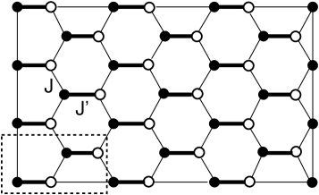
Figure 1: The anisotropic spin-1/2 Heisenberg model investigated in this study.

II Microscopic Model and Corresponding Observables

In this section we introduce the Hamiltonian of the microscopic Heisenberg model as well as some relevant observables. The Heisenberg model considered in this study is defined by the Hamilton operator

$$H=\sum_{\langle xy\rangle}J\,\vec{S}_{x}\cdot\vec{S}_{y}+\sum_{\langle x^{\prime}y^{\prime}\rangle}J^{\prime}\,\vec{S}_{x^{\prime}}\cdot\vec{S}_{y^{\prime}},$$ (1)

where $J^{\prime}$ and $J$ are antiferromagnetic exchange couplings connecting nearest neighbor spins $\langle xy\rangle$ and $\langle x^{\prime}y^{\prime}\rangle$, respectively. Figure 1 illustrates the Heisenberg model described by eq. (1) on the honeycomb lattice with periodic spatial boundary conditions implemented in our simulations. The dashed rectangle in figure 1, which contains $4$ spins, is the elementary cell for building a periodic honeycomb lattice covering a rectangular area. For instance, the honeycomb lattice shown in figure 1 contains 3 $\times$ 3 elementary cells. The honeycomb lattice is not a Bravais lattice. Instead it consists of two triangular Bravais sub-lattices $A$ and $B$ (depicted by solid and open circles in figure 1). As a consequence, the momentum space of the honeycomb lattice is a doubly-covered Brillouin zone of the two triangular sub-lattices. To study the critical behavior of this anisotropic Heisenberg model near the transition driven by the dimerization, in particular to determine the critical exponent $\nu$, several relevant observables are measured in our simulations. A physical quantity of central interest is the staggered susceptibility (corresponding to the third component of the staggered magnetization $M_{s}^{3}$) which is given by

$$\chi_{s} = \frac{1}{L_{1}L_{2}}\int_{0}^{\beta}dt\ \langle M^{3}_{s}(0)M^{3}_{s}(t)\rangle$$ (2)

$$= \frac{1}{L_{1}L_{2}}\int_{0}^{\beta}dt\ \frac{1}{Z}\mbox{Tr}[M^{3}_{s}(0)M^{3}_{s}(t)\exp(-\beta H)].$$

Here $\beta$ is the inverse temperature, $L_{1}$ and $L_{2}$ are the spatial box sizes in the $1$- and $2$-direction, respectively, and $Z=\mbox{Tr}\exp(-\beta H)$ is the partition function. The staggered magnetization order parameter $\vec{M}_{s}$ is defined as $\vec{M}_{s}=\sum_{x}(-1)^{x}\vec{S}_{x}$. Here $(-1)^{x}=1$ on the $A$ sublattice and $(-1)^{x}=-1$ on the $B$ sublattice, respectively. Other relevant quantities calculated from our simulations are the spin stiffnesses in the $1$- and $2$-directions

$$\rho_{si}=\frac{1}{\beta L^{2}_{i}}\langle W^{2}_{i}\rangle,$$ (3)

here $i\in\{1,2\}$ refers to the spatial directions and $W^{2}_{i}$ is the winding number squared in the $i$-direction. Finally, the second-order Binder cumulant for the staggered magnetization, which is defined as

$$Q_{2}=\frac{\langle(M^{3}_{s})^{4}\rangle}{\langle(M^{3}_{s})^{2}\rangle^{2}}$$ (4)

are measured as well. By carefully investigating the spatial volume (and possibly the space-time volume) and the $J^{\prime}/J$ dependence of these observables, one can determine the transition point as well as the critical exponent $\nu$ with high precision.

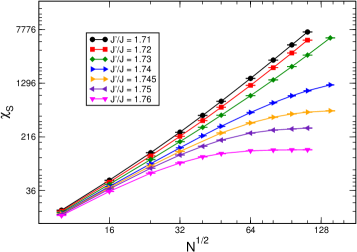
Figure 2: The space-time volume dependence of the staggered susceptibilities $\chi_{s}$ of the Heisenberg model in this work for various values of anisotropy $J^{\prime}/J$. Here $N$ stands for the number of spins. The lines are added to guide the eye.

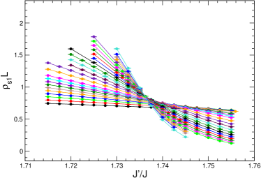
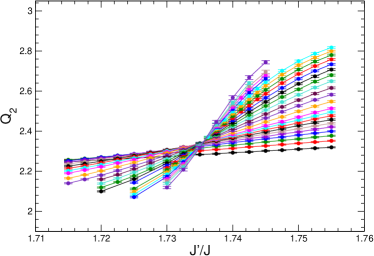
$(a)$	$(b)$

Figure 3: The $J^{\prime}/J$ dependence of $\rho_{s1}L\,\,(a)$ and $Q_{2}\,\,(b)$. The lines are added to guide the eye.

III Determination of the Critical Point and the Critical Exponent $\nu$

The simulations done in this work were performed using the loop algorithm in ALPS library Troyer08 . In order to estimate where in the parameter space $J^{\prime}/J$ the transition occurs, we investigate the space-time volume dependence of the staggered susceptibility $\chi_{s}$. To be more precise, while $\chi_{s}$ grows with increasing space-time volume in the broken phase, in the symmetric phase, $\chi_{s}$ should saturate for large space-time volumes. We further scale $\beta$ with the square root of the number of spins $N$ in order to use this criterion of space-time volume dependence of $\chi_{s}$. Using this criterion, we obtained figure 2. The trend of the curves for different ratios $J^{\prime}/J$ in figure 2 indicates that the transition takes place between $J^{\prime}/J=1.73$ and $J^{\prime}/J=1.74$. Comparing this observation with the related critical point calculated in Wenzel08 for the square lattice case, one sees that the honeycomb lattice has a smaller value of $(J^{\prime}/J)_{c}$. This is reasonable since the antiferromagnet on the honeycomb lattice has a smaller value of the staggered magnetization density $\tilde{{\cal M}_{s}}$ per spin than that on the square lattice Wie94 ; Jia08 . As a result, it is easier to destroy the antiferromagnism on the honeycomb lattice than on the square lattice by increasing the anisotropy $J^{\prime}/J$. Therefore one expects a smaller critical value of $(J^{\prime}/J)_{c}$ on the honeycomb lattice. Further, since phase transition only occurs for a system with infinite degrees of freedom, to investigate the critical behavior of a system on a finite volume, it is useful to employ the idea of finite-size scaling (FSS) hypothesis for certain observables. Pioneering by Fisher in the seventies and generalizing later by Fisher, Barber and others including the derivation of FSS hypothesis from the framework of renormalization group Fisher72 ; Brezin82 ; Barber83 ; Brezin85 , the FSS hypothesis has become the essential method to study the thermodynamic property of a finite system near the phase transition. The characteristic length for a finite system is the correlation length $\xi$. Consequently it is natural to consider its thermodynamics property near the transition as a function of the variable $L/\xi$, where $L$ is the physical size of the system. The FSS hypothesis states that near the transition, any relevant property ${\cal O}_{L}(t)$ of a finite system with critical exponent $\kappa$ can be described by ${\cal O}_{L}(t)=L^{\kappa/\nu}g_{\cal O}(L/\xi)$, where $t$ is given by $t=(j-j_{c})/j_{c}$ with $j=J^{\prime}/J$, $\nu$ is the corresponding critical exponent for $\xi$, and $g_{\cal O}$ is a smooth function. Further, since $\xi$ diverges as $\xi\sim|j-j_{c}|^{-\nu}$ near $j_{c}$, one arrives at ${\cal O}_{L}(t)=L^{\kappa/\nu}g_{\cal O}(Lt^{\nu})=L^{\kappa/\nu}g^{\prime}_{\cal O}(tL^{1/\nu})$, where $g^{\prime}_{\cal O}$ is another smooth function. FSS hypothesis can be rigorously derived by considering the scaling of the relevant directions in the renormalization group flows. They can be understood intuitively as well by assuming the fluctuations of any relevant variable should be invariant at all length scales near $j_{c}$. As a result, the appropriate variable for a finite system near $j_{c}$ is $tL^{1/\nu}$. Here we would like to emphasize that the function ${\cal O}_{L}$ appearing above depends on the lattice geometry as well as the boundary condition. For example, for the Ising model on a 2-D periodic square lattice, there exists a so-called shift exponent $\lambda$ which is related to the deviation of the critical point on a finite volume from the bulk value. For the observables considered in this study, the most relevant FSS ansatz is given by ${\cal O}_{L}(t)=(1+cL^{-\omega})g_{\cal O}(tL^{1/\nu})$, where the confluent correction exponent $\omega$, which arises due to the inhomogeneous part of the free energy as well as the nonlinearity of the scaling field, is included explicitly. One should be aware that above expression of FSS ansatz is an asymptotical one which is valid only for large $L$ and close to $j_{c}$. However to present the main results of this study, we find it is sufficient to employ the FSS ansatz introduced above for the data analysis. As mentioned earlier, when one approaches the critical point $(J^{\prime}/J)_{c}$ for a second order phase transition, the observables $\rho_{s1}3N^{1/2}/2$ and $Q_{2}$ should satisfy the following finite-size scaling formula

$${\cal O}_{L}(t) = (1+cL^{-\omega})g_{\cal O}(tL^{1/\nu})$$ (5)

$$= (1+cL^{-\omega})\Big{[}g_{0}+tL^{1/\nu}g_{1}+(tL^{1/\nu})^{2}g_{2}$$

$$+(tL^{1/\nu})^{3}g_{3}+\dots)\Big{]},$$

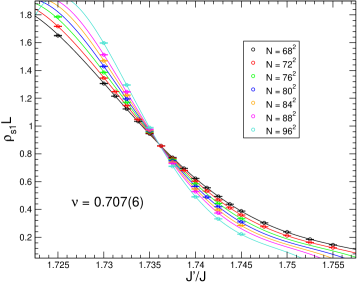
Figure 8: Fit of the numerical data for $\rho_{s1}L$ to their finite-size scaling ansatz with the correction term $cL^{-\omega}$. While the open circles are the Monte Carlo data, the solid lines are obtained by using the results of the fit.

where ${\cal O}$ stands for either $\rho_{s1}3N^{1/2}/2$ or $Q_{2}$, $t=(j-j_{c})/j_{c}$ with $j=J^{\prime}/J$ and $\nu$ and $\omega$ are the corresponding critical exponents introduced before. Further, in eq. (5), $L=3N^{1/2}/2$ or $L=N^{1/2}$ depending on whether the observable ${\cal O}$ is referring to $\rho_{s1}3N^{1/2}/2$ or $Q_{2}$. Finally $g$ is a smooth function of the variable $tL^{\nu}$ and $g_{0}+tL^{1/\nu}g_{1}+(tL^{1/\nu})^{2}g_{2}+(tL^{1/\nu})^{3}g_{3}+\dots$ is the Taylor expansion of the analytic function $g$. From eq. (5), one concludes that if the transition is second order, then the curves of different $L$ should intersect at the critical point for large $L$. In the following, we will employ the finite-size scaling formula eq. (5) for various observables to calculate the critical point as well as the critical exponent $\nu$. After determining the regime where the transition occurs, we have performed substantial simulations with $J^{\prime}/J$ ranging from $J^{\prime}/J=1.715$ to $J^{\prime}/J=1.755$ for $N=10^{2},~{}12^{2},~{}14^{2},\dots,~{}96^{2}$, where $N$ is the total number of spins. We use sufficiently large $\beta$ so that all the observables measured in our simulations take their zero-temperature values. Figure 3 shows the data points for $\rho_{s1}L$ and $Q_{2}$ obtained from the simulations. From the figure, one observes that for both $\rho_{s1}L$ and $Q_{2}$ the curves of different $L$ indeed have a tendency to intersect at one point for large $L$, which in turn is an indications for a second order phase transition. As a first step toward systematically analyzing the data, we would like to have a better estimate of the critical point $(J^{\prime}/J)_{c}$. This can be obtained by investigating the crossing points from either $\rho_{s1}L$ or $Q_{2}$ at system sizes $L$ and $2L$. Figure 4 shows such crossing points as functions of $1/L$. Indeed one sees both crossing points from $\rho_{s1}L$ and $Q_{2}$ approach a common $J^{\prime}/J$ with increasing $L$. By using the analysis suggested in Wan05 , we find that $(J^{\prime}/J)_{c}$ obtained from the upper (lower) crossing points in figure 4 is within the range $(J^{\prime}/J)_{c}\in[1.7345,1.7365]$ ($(J^{\prime}/J)_{c}\in[1.7355,1.7363]$) which agrees with the roughly estimated $(J^{\prime}/J)_{c}$ from $\chi_{s}$. Next, we turn to determine the critical exponent $\nu$ by employing the finite-size scaling ansatz for the observables $\rho_{s1}L$ and $Q_{2}$. First of all, let us focus on $Q_{2}$. A fit of $Q_{2}$ to eq. (5) with $N\geq 12^{2}$ leads to $(J^{\prime}/J)=1.7358(2)$ and $\nu=0.691(2)$. The result is shown in figure 5. In the fits, we carefully make sure that $\nu$ and $(J^{\prime}/J)_{c}$ obtained from the fits are stable, namely $\nu$ and $(J^{\prime}/J)_{c}$ are consistent with respect to the elimination of smaller $N$. For example, from the fit using data points of $N=24^{2}$ to $N=96^{2}$, we find $(J^{\prime}/J)_{c}=1.7357(2)$ and $\nu=0.694(2)$. Both of them agree with the results obtained from the fit using most of the available data points. With $N\geq 26^{2}$, the fits are not stable. This is due to the fact that for large $N$, the data points of $Q_{2}$ are not accurate enough to perform the fits including the term $cL^{-\omega}$ in eq. (5), where the corrections become very small. Therefore we use another approach, namely we use the data with sufficiently large $N$ so that one can safely ignore the correction $cL^{-\omega}$. We also make sure that the results are stable like what we did before. The validity of this strategy is justified as follows. We generate data points from the expression $(1+0.5L^{-b})(1+(tL^{1/c})+0.1(tL^{1/c})^{2}+0.01(tL^{1/c})^{3})$ for various values of $L$ and $t$ with $b=1.5$ and $c=0.8$. By analyzing this set of data, we do observe the convergence of $c$ to $c=0.8$ as one eliminates more data points with smaller value of $L$. Surprisingly, with this strategy we find that for a wide range of $N$ we obtain consistent results with our previous analysis including the correction term $cL^{-\omega}$. For instance, using the data with $N\geq 44^{2}$, we find $\nu=0.693(4)$ which agrees with $\nu=0.691(2)$ obtained earlier (figure 6). At this stage, one naturally would conclude that we find the same unconventional critical behavior as that in Wenzel08 . However, when we use larger $N$, we begin to observe that $\nu$ converges to the expected $O(3)$ value $\nu=0.7112(5)$. For example, fitting the data from $N=60^{2}$ to $N=96^{2}$ to eq. (5) without the term $cL^{-\omega}$ leads to $\nu=0.705(5)$, which is compatible with the expected $O(3)$ value (figure 7). By applying the same analysis to the observable $\rho_{s1}L$, we arrive at similar results. For example, although with a slightly large $\chi^{2}/{\text{d.o.f.}}\sim 5.1$, by fixing $\nu=1.7356$ which is the expected $(J^{\prime}/J)_{c}$ calculated from $Q_{2}$, we find $\nu=0.694(4)$ for $N\geq 48^{2}$ from the fit including the term $cL^{-\omega}$ in eq. (5). We attribute the poor quality of the fit to the correction to the critical point which are not considered here. Indeed with a fixed $(J^{\prime}/J)_{c}=1.7351$ which is not within the the statistical error of $(J^{\prime}/J)_{c}$ obtained from $Q_{2}$, we arrive at $\nu=0.707(3)$ and a better $\chi^{2}/{\text{d.o.f.}}=3.7$. Notice this $\nu$ is even compatible with the known $O(3)$ value. With a fixed $(J^{\prime}/J)_{c}=1.7356$, only from $N\geq 64^{2}$ we begin to obtain $\nu$ consistent with the expected $O(3)$ value $\nu=0.7112(5)$ : by fitting data points with $N\geq 68^{2}$ to eq. (5) with the term $cL^{-\omega}$, we obtain $\nu=0.707(6)$ (figure 8).

Table 1 summarizes the results of all the fits mentioned earlier. We would like to point out that the statistical errors shown in this study are obtained by binning. Hence the error bars presented here might be less accurately determined compared to those calculated with more sophisticated methods. Indeed from the $\chi^{2}/{\text{d.o.f.}}$ shown in table 1, one sees that while the errors for $Q_{2}$ seem to be overestimated, the errors for $\rho_{s1}L$ are likely underestimated. Nevertheless, from the $\chi^{2}/{\text{d.o.f.}}$ presented in table 1, the results we have concluded should remain valid even an optimization procedure is applied for the data analysis. Notice the exponent $\omega$ for the last 2 rows in table 1 are not shown explicitly since the corresponding error bars are of the same magnitude as $\omega$ themselves. This is likely due to the fact that the data is not precise enough to determine $\omega$ unambiguously. Further, the $\omega$ we obtain from the fits are not consistent with the theoretical value. For example, the $\omega$ in the last row of table 1 is $0.38$ which is significantly smaller than the theoretical value $\omega\sim 0.78$. However since the value of $\omega$ will be affected by higher order operators to some extent as well as there might be a strong correlation between $c$ and $\omega$ in formula (5), the $\omega$ presented here should be treated as a effective one. Actually we find that both $\chi^{2}/{\text{d.o.f.}}$ and $\nu$ from the fit of the last row in table 1 are very stable with a fixed value of $\omega$ including $\omega=0.78$. Therefore the result of $\nu=0.707(6)$ shown in table 1 should be trustable.

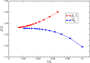
Figure 4: Crossing points of $\rho_{s1}L$ and $Q_{2}$ obtained from the corresponding observables at system sizes $L$ and $2L$. The lines are added to guide the eye.

Observable	$N_{\text{min}}$	$N_{\text{max}}$	$(J^{\prime}/J)_{c}$	$\nu$	$\omega$	$\chi^{2}/{\text{d.o.f.}}$
$Q_{2}$	$12^{2}$	$96^{2}$	$1.7358(2)$	$0.691(2)$	1.98(5)	0.12
$Q_{2}$	$24^{2}$	$96^{2}$	$1.7357(2)$	$0.694(2)$	3.5(6)	0.12
$Q_{2}$	$44^{2}$	$96^{2}$	$1.7356(2)$	$0.693(4)$	-	0.1
$Q_{2}$	$60^{2}$	$96^{2}$	$1.7356(3)$	$0.705(5)$	-	0.08
$\rho_{s1}L$	$48^{2}$	$96^{2}$	$1.7356\,({\text{fixed}})$	$0.694(4)$	0.9(3)	5.1
$\rho_{s1}L$	$48^{2}$	$96^{2}$	$1.7351\,({\text{fixed}})$	$0.707(3)$	-	3.7
$\rho_{s1}L$	$68^{2}$	$96^{2}$	$1.7356\,({\text{fixed}})$	$0.707(6)$	-	1.8

Table 1: Results of the fits mentioned in the text. $N_{\text{min}}$ and $N_{\text{max}}$ refer to the smallest and largest number of spins in the fit, respectively.

IV Discussion and Conclusion

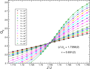
Figure 5: Fit of most of the numerical data points for $Q_{2}$ to their finite-size scaling ansatz including the correction term $cL^{-\omega}$. While the open circles are the Monte Carlo data, the solid lines are obtained by using the results of the fit. Some data points are omitted for better visibility.

In this note, we have performed large scale Monte Carlo simulations to study the critical behavior of the spin-1/2 Heisenberg model with a spatially staggered anisotropy on the honeycomb lattice. In particular, we have demonstrated the subtleties of determining the critical exponent $\nu$ from investigating the finite-size scaling behavior of the relevant observables. From what we have found, we conclude that for the second order phase transition considered here, the large volume data is essential to calculate the corresponding critical exponent $\nu$ correctly. With a detailed data analysis, we find that the critical exponent $\nu$ is given by $\nu=0.707(6)$ which is cosistent with the most accurate $O(3)$ value $\nu=0.7112(5)$ obtained in Cam02 . By including the sub-leading correction in the finite-size scaling ansatz and using most of the available data points, we can obtain a value of $\nu$ consistent with that calculated in Wenzel08 . Concerning the finite volume effect, we believe the $\nu$ obtained from using only large $N$ is more reliable. Our results do not necessarily imply that the critical exponent $\nu$ obtained in Wenzel08 should not be trusted. However from what we have found in this study, it would be desirable to go beyond the volumes used in Wenzel08 to see whether the unconventional behavior observed in Wenzel08 will continue to hold with the addition of larger volumes or not.

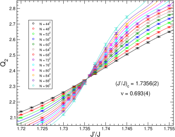
Figure 6: Fit of $Q_{2}$ to its finite-size scaling ansatz given by eq. (5) without taking the correction $cL^{-\omega}$ into account. The number of spins $N$ used in the fit ranges from $44^{2}$ to $96^{2}$. While the open circles are the Monte Carlo data, the solid lines are obtained by using the results of the fit.

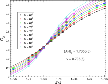
Figure 7: Fit of the numerical data for $Q_{2}$ to their finite-size scaling ansatz without the correction term $cL^{-\omega}$ in eq. (5). The number of spins $N$ used in the fit ranges from $N=60^{2}$ to $N=96^{2}$. While the open circles are the Monte Carlo data, the solid lines are obtained by using the results of the fit.

V acknowledgments

We like to thank U.-J. Wiese for useful discussions. This work is supported in part by funds provided by the Schweizerischer Nationalfonds (SNF). The “Center for Research and Education in Fundamental Physics” at Bern University is supported by the “Innovations- und Kooperationsprojekt C-13” of the Schweizerische Universitätskonferenz (SUK/CRUS).

References

- (1) S. Wenzel, L. Bogacz, and W. Janke, Phys. Rev. Lett. 101, 127202 (2008).
- (2) U.-J. Wiese and H.-P. Ying, Z. Phys. B 93, 147 (1994).
- (3) A. Parola, S. Storella, and Q. F. Zhong, Phys. Rev. Lett. 71, 4393 (1993).
- (4) I. Affleck and B. I. Halperin, Journal of Physics A: Mathematical and General 29, 2627 (1996).
- (5) A. W. Sandvik, Phys. Rev. Lett. 83, 3069 (1999).
- (6) V. Y. Irkhin and A. A. Katanin, Phys. Rev. B 61, 6757 (2000).
- (7) Y. J. Kim and R. Birgeneau, Phys. Rev. B 62, 6378 (2000).
- (8) V. Hinkov et al., Nature Physics 3, 780 (2007).
- (9) V. Hinkov et al., Science 319, 597 (2008).
- (10) T. Pardini, R. R. P. Singh, A. Katanin and O. P. Sushkov, Phys. Rev. B 78, 024439 (2008).
- (11) F.-J. Jiang, F. Kämpfer, and M. Nyfeler, Phys. Rev. B 80, 033104 (2009).
- (12) A. F. Albuquerque, M. Troyer, and J. Oitmaa, Phys. Rev. B 78, 132402 (2008).
- (13) S. Wenzel and W. Janke, Phys. Rev. B 79, 014410 (2009).
- (14) M. Campostrini, M. Hasenbusch, A. Pelissetto, P. Rossi, and E. Vicari, Phys. Rev. B 65, 144520 (2002).
- (15) F.-J. Jiang, F. Kämpfer, M. Nyfeler, and U.-J. Wiese, Phys. Rev. B 78, 214406 (2008).
- (16) L. Wang, K. S. D. Beach, and A. W. Sandvik, arXiv:cond-mat/0509747.
- (17) A. F. Albuquerque et al., Journal of Magnetism and Magnetic Material 310, 1187 (2007).
- (18) M. E. Fisher and M. N. Barber, Phys. Rev. Lett. 28, 1516 (1972).
- (19) E. Brézin, J. Phys. (Paris) 43, 15 (1982).
- (20) M. N. Barber, in Phase Transitions and Critical Phenomena, ed. C. Domb (Academic, New York, 1983), Vol. 8.
- (21) E. Brézin and J. Zinn-Justin, Nucl. Phys. B 257, 867 (1985).