Measurement-based quantum phase estimation algorithm for finding eigenvalues of non-unitary matrices

Abstract

We propose a quantum algorithm for finding eigenvalues of non-unitary matrices. We show how to construct, through interactions in a quantum system and projective measurements, a non-Hermitian or non-unitary matrix and obtain its eigenvalues and eigenvectors. This proposal combines ideas of frequent measurement, measured quantum Fourier transform, and quantum state tomography. It provides a generalization of the conventional phase estimation algorithm, which is limited to Hermitian or unitary matrices.

I Introduction

One of the most important tasks for a quantum computer would be to efficiently obtain eigenvalues and eigenvectors of high-dimensional matrices. It has been suggested abrams that the quantum phase estimation algorithm (PEA) Kitaev95 can be used to obtain eigenvalues of a Hermitian matrix or Hamiltonian. For a quantum system with a Hamiltonian $H$, a phase factor, which encodes the information of eigenvalues of $H$, is generated via unitary evolution $U=\exp(-iH\tau)$. By evaluating the phase, we can obtain the eigenvalues of $H$. The conventional PEA consists of four steps: preparing an initial approximated eigenstate of the Hamiltonian $H$, implementing unitary evolution operation, performing the inverse quantum Fourier transform (QFT), and measuring binary digits of the index qubits.

The PEA is at the heart of a variety of quantum algorithms, including Shor’s factoring algorithm chuang . A number of applications of PEA have been developed, including generating eigenstates associated with an operator tm , evaluating eigenvalues of differential operators szk , and it has been generalized using adaptive measurement theory to achieve a quantum-enhanced measurement precision at the Heisenberg limit hig . The PEA with delays considering the effects of dynamical phases has also been discussed wei . The implementation of an iterative quantum phase estimation algorithm with a single ancillary qubit is suggested as a benchmark for multi-qubit implementations mir . The PEA has also been applied in quantum chemistry to obtain eigenenergies of molecular systems aa ; whf . This application has been demonstrated in a recent experiment expt . Moreover, several proposals have been made to estimate the phase of a quantum circuit Ngpra , and the use of phase estimations for various algorithms Ng1 ; Ng2 , including factoring and searching.

The conventional PEA is only designed for finding eigenvalues of either a Hermitian or a unitary matrix. In this paper, we propose a measurement-based phase estimation algorithm (MPEA) to evaluate eigenvalues of non-Hermitian matrices. This provides a potentially useful generalization of the conventional PEA. Our proposal uses ideas from conventional PEA, frequent measurement, and techniques in one-qubit state tomography. This proposal can be used to design quantum algorithms apart from those based on the standard unitary circuit model. The proposed quantum algorithm is designed for systems with large dimension, when the corresponding classical algorithms for obtaining the eigenvalues of the non-unitary matrices become so expensive that it is impossible to implement on a classical computer.

The structure of this work is as follows: In Sec. II we introduce how to construct a non-Hermitian evolution matrix for a quantum system. In Sec. III, we present the measurement-based phase estimation algorithm, introducing two methods for obtaining the complex eigenvalues of the non-Hermitian evolution matrix. We give two examples for the application of MPEA and discuss how to construct Hamiltonian for performing the controlled unitary operation in Sec. IV. In Sec. V, we discuss the success probability of the algorithm and the efficiency of constructing the non-Hermitian matrix. We close with a conclusion section.

II Constructing non-unitary matrices

Now we describe how to construct non-unitary matrices on a quantum system. A bipartite system, composed of subsystems A and B, evolves under Hamiltonian

$$H=H_{A}+H_{B}+H_{AB},$$ (1)

where $H_{A~{}(B)}$ is the Hamiltonian of subsystem A(B) and $H_{AB}$ is their interaction. We prepare the initial state of subsystem A in its pure state $|\varphi_{A}\rangle\langle\varphi_{A}|$ and the initial state of subsystem B in an arbitrary state $\rho_{B}$. Then at time $t=0$, the state of the system is $\rho_{0}=|\varphi_{A}\rangle\langle\varphi_{A}|\otimes\rho_{B}$. Let the system evolve under the Hamiltonian $H$ for a time interval $\tau$, if subsystem A is subject to a projective measurement $M=|\varphi_{A}\rangle\langle\varphi_{A}|$ applied at time interval $\tau$, this is equivalent to driving subsystem B with an evolution matrix

$$V_{B}(\tau)\equiv\langle\varphi_{A}|\exp\left(-iH\tau\right)|\varphi_{A}\rangle.$$ (2)

This evolution matrix is in general neither unitary nor Hermitian.

The Hamiltonian $H$ of the whole quantum system can be spanned as:

$$H=\sum_{j=1}^{D}E_{j}|E_{j}\rangle\langle E_{j}|,$$ (3)

with eigenenergies $E_{j}$, and the corresponding eigenvectors $|E_{j}\rangle$ can be spanned in terms of tensor products of basis vectors {$|\psi_{k}^{A}\rangle$} and {$|\psi_{r}^{B}\rangle$} of Hilbert spaces of subsystems A and B, which are of dimensions $D_{A}$ and $D_{B}$, respectively, and $D=D_{A}\times D_{B}$. Using the bases for A and B, we have

$$|E_{j}\rangle=\sum_{k=1}^{D_{A}}\sum_{r=1}^{D_{B}}f_{kr}^{j}|\psi_{k}^{A}\rangle\otimes|\psi_{r}^{B}\rangle,$$ (4)

and the evolution matrix on subsystem B, after the measurement $M$ performed on subsystem A at time interval $\tau$, becomes

$$V_{B}(\tau)=\langle\varphi^{A}|e^{-iH\tau}|\varphi^{A}\rangle=\sum_{r,s=1}^{D_{B}}V_{rs}|\psi_{r}^{B}\rangle\langle\psi_{s}^{B}|,$$ (5)

where

$$V_{rs}=\sum_{j=1}^{D}e^{-iE_{j}\tau}\sum_{k,l=1}^{D_{A}}f_{kr}^{j}f_{ls}^{j\ast}c_{k}^{A}c_{l}^{A\ast},$$ (6)

and

$$c_{k}^{A}=\langle\varphi^{A}|\psi_{k}^{A}\rangle.$$ (7)

More generally, we can construct different evolution matrices by performing measurements on subsystem A with different time intervals and/or different measurement bases. For example, by sequentially performing projective measurements with time intervals $\tau_{1}$, $\tau_{2}$, $\tau_{3}$, an evolution matrix

$$V_{B}(\tau_{1},\tau_{2},\tau_{3})=V_{B}(\tau_{3})V_{B}(\tau_{2})V_{B}(\tau_{1})$$ (8)

is constructed. We can also combine unitary evolution matrices with the non-unitary transformations on subsystem B to construct some desired evolution matrices.

III Measurement-based quantum phase estimation algorithm

For the bipartite system, set the initial state of the system in a separable state

$$\rho_{0}=|\varphi_{A}\rangle\langle\varphi_{A}|\otimes\rho_{B},$$ (9)

and let the system evolve under the Hamiltonian in Eq. ($1$). Then after performing $m$ successful projective measurements on subsystem A with time intervals $\tau$, the evolution on the Hilbert space of subsystem B is driven by $\left[V_{B}(\tau)\right]^{m}$, and the state of subsystem B evolves to nakazato

$$\rho_{B}^{(\tau)}(m)=\frac{\bigl{[}V_{B}(\tau)\bigr{]}^{m}\rho_{B}\bigl{[}V_{B}^{\dagger}(\tau)\bigr{]}^{m}}{P^{\left(\tau\right)}\left(m\right)},$$ (10)

where

$$P^{\left(\tau\right)}\left(m\right)=\text{Tr}_{B}\bigl{\{}[V_{B}(\tau)]^{m}\rho_{B}[V_{B}^{\dagger}(\tau)]^{m}\bigr{\}}$$ (11)

is the probability of finding subsystem A still in state $|\varphi_{A}\rangle$ after each of the $m$ measurements.

The evolution matrix $V_{B}(\tau)$ can be spanned as

$$V_{B}(\tau)=\sum_{k}\lambda_{k}|u_{k}\rangle\langle v_{k}|,$$ (12)

where $|u_{k}\rangle$ and $\langle v_{k}|$ are the right- and left-eigenvectors of $V_{B}(\tau)$ and $\lambda_{k}$ is the corresponding eigenvalue nakazato satisfying $0\leq|\lambda_{k}|\leq 1$. In the large $m$ limit, the operator $[V_{B}(\tau)]^{m}$ is dominated by a single term $\lambda_{\max}^{m}|u_{\max}\rangle\langle v_{\max}|$, provided the largest eigenvalue $\lambda_{\max}$ is unique, discrete, and non-degenerate. In the limit of large $m$ and finite $\tau$, $\rho_{B}^{(\tau)}(m)$ tends to a pure state, independent of the initial (mixed) state of subsystem B. The final state of $\rho_{B}^{(\tau)}(m)$ is dominated by $|u_{\max}\rangle$, and this outcome is found with probability nakazato

$$P^{\left(\tau\right)}\left(m\right)\longrightarrow|\lambda_{\max}|^{2m}\langle u_{\max}|u_{\max}\rangle\langle v_{\max}|\rho_{B}|v_{\max}\rangle.$$ (13)

The state of subsystem B evolves to $|u_{\max}\rangle$, after performing a number of operations of $V_{B}(\tau)$. Then we can evaluate $\lambda_{\max}$ by resolving the phase of the state. If we prepare the initial state of subsystem B in a pure initial state that is close to an eigenstate of the matrix $V_{B}(\tau)$, the state of the subsystem B can evolve to other eigenstates of $V_{B}$. Then we can also obtain the corresponding eigenvalues of $V_{B}(\tau)$.

Based on the above analysis, we suggest a measurement-based phase estimation algorithm for evaluation of the eigenvalues of the matrix $V_{B}(\tau)$. As in the circuit shown in Fig. $1$($a$), three quantum registers are prepared. From top to bottom: an index register, a target register and an interacting register. The index register is a single qubit, which is used as control qubit and to readout the final results for the eigenvalues; the target register is used to represent the state $\rho_{B}$ of subsystem B; and the interacting register represents the state $|\varphi_{A}\rangle$ of subsystem A.

The initial state of the circuit is prepared in the state

$$|0\rangle\langle 0|\otimes\rho_{B}\otimes|\varphi_{A}\rangle\langle\varphi_{A}|,$$ (14)

with subsystem A in a pure state $|\varphi_{A}\rangle\langle\varphi_{A}|$, and subsystem B in state $\rho_{B}$. The construction of the controlled evolution matrix $V_{B}(\tau)$ on the target register is achieved by implementing the controlled unitary ($C$-$U$) transformation for the whole quantum system and successfully performing the projective measurement $M=|\varphi_{A}\rangle\langle\varphi_{A}|$ on the interacting register with time interval $\tau$. Note here for the unitary transformation $U=\exp\left({-iHt}\right)$, we set $t$ such that $m$ projective measurements are performed successfully on subsystem $A$ at the time interval $\tau$, while the unitary transformation of the whole system evolves for time period $t$. After performing $m$ successful periodic measurements on the interacting register with time intervals $\tau$, as shown in Fig. $1$($b$), the state of the system is transformed to

$$\frac{1}{2}\biggl{\{}|0\rangle\langle 0|\otimes\rho_{B}+|1\rangle\langle 1|\otimes\bigl{[}V_{B}(\tau)\bigr{]}^{m}\rho_{B}\bigl{[}V_{B}^{\dagger}(\tau)\bigr{]}^{m}\biggr{\}}$$

$$\otimes|\varphi_{A}\rangle\langle\varphi_{A}|.$$ (15)

The dominant term of this is

$$\frac{1}{\sqrt{2}}\biggl{[}|0\rangle+(\lambda_{\max})^{m}|1\rangle\biggr{]}|u_{\max}\rangle|\varphi_{A}\rangle,$$ (16)

and the state of the index qubit is dominated by

$$|\psi_{\text{ind}}\rangle=\frac{1}{\sqrt{2}}\biggl{[}|0\rangle+(\lambda_{\max})^{m}|1\rangle\biggr{]}.$$ (17)

In general, $\lambda_{\max}$ is a complex number and can be written as

$$\lambda_{\max}=\exp\left(i\varphi\right)=\exp\left[i\left(a+ib\right)\right].$$ (18)

We can obtain $\lambda_{\max}$ by resolving the phase factor

$$\varphi=(a+ib).$$ (19)

Two approaches can be used to resolve $\lambda_{\max}$: $\left(i\right)$ using single-qubit quantum state tomography (QST) kwiat , and $\left(ii\right)$ using the measured quantum Fourier transform (mQFT) combined with projective measurements on a single qubit. The details of these two approaches are given below.

III.1 Approach using single-qubit state tomography

Quantum state tomography can fully characterize the quantum state of a particle or particles through a series of measurements in different bases kwiat ; liu . In the approach using QST to resolve the eigenvalue of the matrix $V_{B}(\tau)$, we prepare a large number of identical copies of the state on the index qubit $|\psi_{\text{ind}}\rangle$, as shown in Eq. ($17$), by running the MPEA circuit a number of times. Then the value of $\lambda_{\max}$ can be obtained by determining the index qubit state.

The state of the index qubit in Eq. ($17$) can be written as

$$|\psi_{\text{ind}}\rangle=\frac{1}{\sqrt{2}}\bigl{(}|0\rangle+\exp\left[m\left(-b+ia\right)\right]|1\rangle\bigr{)}.$$ (20)

In the QST approach, we perform a projective measurement on the index qubit in the basis $|1\rangle\langle 1|$ to obtain the probability of finding the index qubit in state $|1\rangle$, thus obtaining the value of $b$. With the knowledge of $b$, then perform a $\pi/2$ rotation around the $x$-axis and a measurement in the basis of the Pauli matrix $\sigma_{z}$ on the index qubit, we can obtain the observable

$$\langle\psi_{\text{ind}}|\exp\left(-i\frac{\pi}{4}\sigma_{x}\right)\sigma_{z}\exp\left(i\frac{\pi}{4}\sigma_{x}\right)|\psi_{\text{ind}}\rangle$$ (21)

and thus obtain the value of $a$.

The measurement errors of QST, from counting statistics, obey the central limit theorem. To obtain more accurate results, we have to prepare a larger ensemble of the single qubit states.

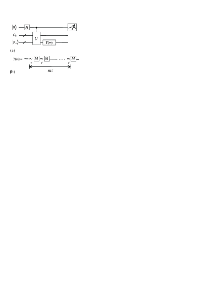
Figure 1: Quantum circuit for measurement-based phase estimation algorithm (MPEA) using quantum state tomograph (QST) approach. Part ($a$) shows the circuit for the MPEA using QST. From top to bottom, an index register, a target register and an interacting register are prepared in the states $|0\rangle$, $\rho_{B}$, and $|\varphi_{A}\rangle$, respectively. The index register is a single qubit used as control qubit; the target register is used to represent the state of subsystem B; and the interacting register is used to represent the state of subsystem A, which interacts with B. Part ($b$) shows the circuit for performing $m$ projective measurements with period $\tau$. In the circuit, the unitary transformation $U=\exp(-iHt)$, we set $t$ such that $m$ projective measurements are performed successfully on subsystem A separated by a time interval $\tau$, while the unitary transformation of the whole system evolves for time $t$.

III.2 Approach using measured quantum Fourier transform combined with projective measurements

In the second approach, we use the techniques of measured quantum Fourier transform and projective measurements to resolve the eigenvalue of the matrix $V_{B}(\tau)$. The phases which encode the eigenvalues of $V_{B}(\tau)$ are in general complex numbers; the inverse QFT can be used to resolve the real part $a$ of the phase $\varphi=(a+ib)$. The imaginary part $b$ of the phase factor, $\varphi$, can be obtained by performing single-qubit projective measurements. The details of this method are discussed below.

In order to resolve $a$ up to $n$ binary digits using the inverse QFT, one has to construct a series of controlled evolution matrices, $C$-$V_{B}(\tau)$, in successive binary powers, from $(n-1)$ to $0$. In the MPEA, this is done by implementing the $C$-$U$ operation on the whole system and performing a series of $2^{k}$ periodic measurements separated by time intervals $\tau$ for $k=(n-1),(n-2),\cdots,0$, respectively. The $C$-$U$ operation evolves for a time $t$, during which all the measurements are performed successfully on the interacting register. Then we can obtain a series of controlled transformation matrices in binary powers, $C$-$[V_{B}(\tau)]^{2^{k}},$ $k=(n-1),$ $(n-2),\cdots,$ $0$. In Fig. $2$($c$), we show the circuit for the $k$th projective measurement with period $\tau$, $W(k)$, where the measurement $M=|\varphi_{A}\rangle\langle\varphi_{A}|$ is performed $2^{k}$ times with period $\tau$ on the interacting register, while the whole system evolves under the controlled unitary operation $U$. The measurements on the interacting register are sequentially performed $W(n-1),W(n-2),\cdots,W(0)$. Then, correspondingly, on the index qubit, we obtain single qubit states as

$$\frac{1}{\sqrt{2}}\biggl{[}|0\rangle+(\lambda_{\max})^{2^{(n-1)}}|1\rangle\biggr{]},\frac{1}{\sqrt{2}}\biggl{[}|0\rangle+(\lambda_{\max})^{2^{(n-2)}}|1\rangle\biggr{]},$$

$$\cdots,\frac{1}{\sqrt{2}}\bigl{(}|0\rangle+\lambda_{\max}|1\rangle\bigr{)}.$$ (22)

Afterward, we can retrieve $n$ binary digits of the real part $a$ of the phase factor $\varphi$, of $\lambda_{\max}$, by performing a mQFT.

The mQFT technique implements a QFT using only a single qubit PP ; niu . It uses the fact that gates within the Fourier transform are applied sequentially on qubits. This modification of the QFT algorithm preserves the probabilities of all measurements niu . The procedure for obtaining the real part of the phase factor of $\lambda_{\max}$ by using mQFT is shown in Fig. $2$($a$), where the circuit in the dotted square is replaced by circuits in the dotted squares shown in Fig. $2$($b$), sequentially obtaining $n$ binary digits of $a$. The details of this procedure are shown below.

The initial state of the MPEA circuit is prepared as in Eq. ($14$). After performing the $k$th periodic measurements $W(k)$ on the interacting register, the dominant term of the state of the system becomes

$$\frac{1}{\sqrt{2}}\bigg{[}|0\rangle+\lambda_{\max}^{2^{k}}|1\rangle\bigg{]}|u_{\max}\rangle|\varphi_{A}\rangle.$$ (23)

The state of the index qubit can be written as

$$|\psi_{\text{ind}}\rangle = \frac{1}{\sqrt{2}}\biggl{[}|0\rangle+\exp\left(i(a+ib)2^{k}\right)|1\rangle\biggr{]}$$ (24)

$$= \frac{1}{\sqrt{2}}\biggl{[}|0\rangle+\exp\left(-b2^{k}\right)\exp\left(ia2^{k}\right)|1\rangle\biggr{]}.$$

In order to resolve the real part $a$ of the phase factor, $\varphi$, we first need to obtain the value of $b$, the imaginary part of the phase factor. This can be achieved by using a single-qubit projective measurement. One can prepare an ensemble of $|\psi_{\text{ind}}\rangle$ and perform projective measurements $|1\rangle\langle 1|$. The value of $b$ can be obtained through the probability for observing the index qubit in state $|1\rangle$.

Let

$$r_{k}=\frac{1}{\sqrt{2}}\biggl{[}1+\exp\left(-b2^{k+1}\right)\biggr{]}^{1/2},$$ (25)

and let us run MPEA again and perform a single qubit operation $Q_{k}$ on the index qubit such that the index qubit is rotated to state

$$|\psi_{\text{ind}}^{\prime}\rangle=r_{k}\frac{1}{\sqrt{2}}\biggl{[}|0\rangle+\exp\left(ia2^{k}\right)|1\rangle\biggr{]},$$ (26)

where the single-qubit operation $Q_{k}$ is defined as

$$Q_{k}=q_{k}\left(\begin{array}[]{cc}1+e^{b2^{k}}&e^{-ia2^{k}}\left(1-e^{b2^{k}}\right)\\ e^{ia2^{k}}\left(e^{b2^{k}}-1\right)&1+e^{b2^{k}}\end{array}\right),$$ (27)

where $q_{k}=1/\sqrt{2\left[1+\exp\left(b2^{k+1}\right)\right]}$. Then we apply the mQFT technique to resolve the real part $a$ of the phase factor $\varphi=(a+ib)$. We therefore obtain the eigenvalue $\exp\bigl{[}i(a+ib)\bigr{]}$ of the matrix $V_{B}(\tau)$.

In the MPEA, the $n$th binary digit of the phase factor is retrieved first, and the partial measurement on the interacting register is performed in sequence of $2^{n-1},2^{n-2}$ to $2^{0}$ times. This procedure provides high fidelity for the state of the target register since each measurement drives the state of the target register closer to $|u_{\max}\rangle$, the eigenstate of $V_{B}(\tau)$.

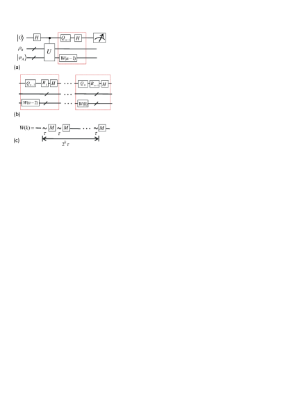
Figure 2: Quantum circuit for a measurement-based phase estimation algorithm (MPEA) using measured quantum Fourier transformation. Part (a) shows the circuit for the MPEA. From top to bottom, an index register, a target register and an interacting register are prepared in the states $(|0\rangle+|1\rangle)/\sqrt{2}$, $\rho_{B}$, and $|\varphi_{A}\rangle$, respectively. The index register is a single qubit used as control qubit and to perform mQFT; the target register is used to represent the state of subsystem B; and the interacting register is used to represent the state of subsystem A, which interacts with B. The circuit in the dotted square in (a) is used for obtaining the $n$th binary digit of the real part of the phase factor. In part (b), a sequence of circuits inside the dashed squares is used to replace the circuit in the dashed square in part ($a$), in order to resolve from the ($n-1$)th to the first binary digits of the real part of the phase factor. Here, $H$ is the Hadamard gate, $Q_{k}$ is a single-qubit rotation as defined in Eq. ($27$) and $R_{k}$ is a single-qubit rotation in quantum Fourier transform. Part (c) shows the circuit for the “$k$th” partial measurement $W(k)$ with period $\tau$. In the circuit, for the unitary transformation $U=\exp(-iHt)$, we set $t$ such that all projective measurements are performed successfully on subsystem A while the unitary transformation of the whole system evolves for time $t$.

IV Examples of measurement-based phase estimation

IV.1 Phase estimation for the Jaynes-Cummings Hamiltonian

Now we use a simple model to show how MPEA works. We consider here a quantum system consisting of two subsystems A and B, where B contains two non-interacting spin qubits, B${}_{\text{1}}$ and B${}_{\text{2}}$; and subsystem A is a photon. The whole system is described by the Jaynes-Cummings Hamiltonian wu

$$H=w_{0}b^{{\dagger}}b+w_{1}(\sigma_{1}^{z}+\sigma_{2}^{z})+\frac{J}{2}[b(\sigma_{1}^{+}+\sigma_{2}^{+})+b^{\dagger}(\sigma_{1}^{-}+\sigma_{2}^{-})],$$ (28)

where $b$ ($b^{\dagger}$) is a bosonic annihilation (creation) operator of the photons. Consider the case $w_{0}=w_{1}$, and perform projective measurements in the basis of a single photon state $|\varphi_{A}\rangle=|1\rangle$. Then we have

$$V_{B}(\tau) = \text{diag}\biggl{\{}1,\bigl{[}3+2\cos(\sqrt{10}\tau J)\bigr{]}/5\times e^{-2iw_{0}\tau},$$ (29)

$$\cos(\sqrt{6}\tau J)e^{-iw_{0}\tau},\cos(\sqrt{2}\tau J)\biggr{\}},$$

in the ordered basis $\bigl{\{}|1,s\rangle,|1,t_{+}\rangle,|1,t_{0}\rangle,|1,t_{-}\rangle\bigr{\}}$, where

$$|s\rangle = \frac{1}{\sqrt{2}}(|01\rangle-|10\rangle),\text{ \ \ }|t_{+}\rangle=|11\rangle,$$

$$|t_{0}\rangle = \frac{1}{\sqrt{2}}(|01\rangle+|10\rangle),\text{ \ \ }|t_{-}\rangle=|00\rangle.$$ (30)

Let $\tau=1/2$ and $w_{0}=w_{1}=J=1$, then we construct an evolution matrix $V_{B}(\tau)$ as

$$V_{B}(\tau) = \text{diag}\biggl{\{}1,\bigl{[}3+2\cos(\sqrt{10}/2)\bigr{]}/5\times e^{-i},$$ (31)

$$\cos(\sqrt{6}/2)e^{-i/2},\cos(\sqrt{2}/2)\biggr{\}}.$$

On the MPEA circuit, now let us prepare the target register in a mixed state:

$$\rho_{B}=\frac{1}{4}\biggl{(}|s\rangle\langle s|+|t_{+}\rangle\langle t_{+}|+|t_{0}\rangle\langle t_{0}|+|t_{-}\rangle\langle t_{-}|\biggr{)},$$ (32)

and the interacting register in state $|\varphi_{A}\rangle=|1\rangle$. Then implement the controlled Hamiltonian of Eq. ($28$) for a time $t$ during which the projective measurements on the interacting register are performed successfully. After a series of projective measurements, in the basis of $|\varphi_{A}\rangle=|1\rangle$, on the interacting register, the state of the target register evolves to a singlet state $|s\rangle$, which corresponds to the largest eigenvalue of $V_{B}(\tau)$. We resolve the corresponding phase as zero, thus its eigenvalue is one. The survival probability, $P^{\left(\tau\right)}\left(m\right)$, of the state $|\varphi_{A}\rangle=|1\rangle$ on the interacting register after $m$ successful measurements, and the fidelity, $F^{\left(\tau\right)}(m)$, for the target register to be in state $|u_{\max}\rangle$, are shown in Fig. $3$. The fidelity $F^{\left(\tau\right)}(m)$ is defined as

$$F^{\left(\tau\right)}\left(m\right)=\frac{\langle u_{\max}|\rho_{B}^{(\tau)}(m)|u_{\max}\rangle}{\langle u_{\max}|u_{\max}\rangle}$$ (33)

Since $F^{\left(\tau\right)}\left(m\right)$ is close to one, the success probability is determined by $P^{\left(\tau\right)}\left(m\right)$.

Figure 3: Survival probability $P(m)$ ($\blacktriangle$) and fidelity $F(m)$ ($\bullet$) for $|\varphi_{A}\rangle=|1\rangle$ versus $m$, the number of successful measurement, for the Jaynes-Cummings model.

If we prepare the target register in a pure initial state that is close to an eigenstate of the matrix $V_{B}$, by applying MPEA, the state of the target register can evolve to other eigenstates of $V_{B}$. Then we can also obtain the corresponding eigenvalues of $V_{B}$.

For example, applying MPEA to the above system and preparing the target register in state $|t_{+}\rangle$, by performing projective measurements with $|\varphi_{A}\rangle=|1\rangle$ on the interacting register, the state of the target register would remain in the $|t_{+}\rangle$ state. We can retrieve the real part of the phase factor of the corresponding eigenvalue up to an accuracy of $2$, $8$ and $16$ binary digits, respectively, and obtain the eigenvalues of the matrices $V_{B}$ as $\exp[-0.5177-i2\pi(0.25\pm 0.25)]$, $\exp[-0.5177-i2\pi(0.160\pm 0.008)]$, and $\exp[-0.5177-i2\pi(0.15918\pm 0.00003)]$, assuming we have already obtained the imaginary part of the eigenvalue of $V_{B}$ through projective measurements. The true eigenvalue is $\exp(-0.5177-i)$, which is quite close.

To implement a controlled unitary evolution on the MPEA circuit, we set the control qubit as a single spin and label it as subsystem C. Thus, the controlled Hamiltonian of the whole system becomes

$$\widetilde{H} = \frac{1}{2}(1-\sigma_{C}^{Z})H=\frac{1}{2}(1-\sigma_{C}^{Z})\biggl{\{}w_{0}b^{{\dagger}}b+w_{1}(\sigma_{1}^{z}+\sigma_{2}^{z})+$$ (34)

$$\frac{J}{2}\big{[}b(\sigma_{1}^{+}+\sigma_{2}^{+})+b^{\dagger}(\sigma_{1}^{-}+\sigma_{2}^{-})\big{]}\biggr{\}}.$$

This Hamiltonian contains three-body interactions and cannot be implemented directly. One could decompose the three-body interaction into two-body interactions som ; tseng and then implement the two-body interaction. In general, an arbitrary unitary matrix $U=\exp\left(-iHt\right)$ can be decomposed mot ; kha into tensor products of unitary matrices of $4\times 4$ and $2\times 2$, which correspond to two- and single-qubit operations respectively, and can be implemented on a universal quantum computer.

IV.2 Phase estimation for the axial symmetry model

For another example, we consider the axial symmetry model wu . This is relevant for quantum information processing in solid state moz ; ima ; qui and atomic zheng systems. The quantum system is composed of two subsystems A and B, where B contains two non-interacting spins, and subsystem A contains a single spin interacting with subsystem B. The Hamiltonian for the whole system is wu

$$H=\frac{J}{2}\bigl{[}X(X_{1}+X_{2})+Y(Y_{1}+Y_{2})\bigr{]},$$ (35)

where $X$ and $Y$ are the Pauli operators. By performing projective measurements on subsystem A in the basis of the $\sigma_{z}$-eigenvector, then in the basis $\{|s\rangle,|t_{+}\rangle,|t_{0}\rangle,|t_{-}\rangle\}$, we obtain

$$V_{B}(\tau)=\text{diag}\biggl{\{}1,1,\cos\left(\sqrt{2}\tau J\right),\cos\left(\sqrt{2}\tau J\right)\biggr{\}},$$ (36)

operating on subsystem B. If we prepare the initial state of the target register in state $|t_{0}\rangle$, then the fidelity of the target register to be in state $|t_{0}\rangle$ is $1$ after performing a number of successful measurements on the interacting register. For the case $J=2$ and $\tau=1$, the corresponding eigenvalue is $-0.951363$. The success probability of the successful measurement on the interacting register versus the number of measurements on the interacting register is shown in Fig. $4$. From that figure, we can see that even for $10$ successful measurements, we can still have a success probability of $0.37$.

Figure 4: Survival probability $P(m)$ for $|\varphi_{A}\rangle=|1\rangle$ versus $m$, the number of successful measurements, by using the $\sigma_{z}$-eigenstate as the measurement basis for the axial symmetry model.

V Discussion

On a quantum computer, a unitary matrix can be efficiently represented, i.e., for a unitary matrix of dimension $2^{s}$, only $s$ qubits are needed to represent it on a quantum computer. In this paper, we have tried to represent a non-unitary matrix on a quantum system by performing periodic projective measurements. Whether an arbitrary matrix can be constructed using this technique still remains an open problem, and this would be a subject for future study.

V.1 Implementation of the controlled nonunitary transformation

In the conventional PEA, the phase factor is resolved through a quantum Fourier transform. To resolve the binary expansion of the phase, up to $n$ binary digits, one has to implement $n$ controlled unitary transformations in successive binary powers: $C$-$U^{2^{n-1}}$, $C$-$U^{2^{n-2}},\cdots,C$-$U^{2^{0}}$.

In the MPEA approach of using mQFT combined with projective measurements to obtain the eigenvalues of $V_{B}$, we need to implement the controlled transformations in successive binary powers: $C$-$V_{B}^{2^{n-1}}\!\left(\tau\right)$, $C$-$V_{B}^{2^{n-2}}\!\left(\tau\right),\cdots,C$-$V_{B}^{2^{0}}\!\left(\tau\right)$, and followed by the corresponding mQFT circuit as shown in Fig. $2$. The controlled transformations $C$-$V_{B}^{2^{n-1}}\!\left(\tau\right)$, $C$-$V_{B}^{2^{n-2}}\!\left(\tau\right)$, $\cdots$, $C$-$V_{B}^{2^{0}}\!\left(\tau\right)$, are achieved by implementing the controlled Hamiltonian on the whole system only once and during a time $t$ until the successful measurements on the interacting register finish, and performing measurements $W(n-1),W(n-2),\cdots,W(0)$, i.e., a series of periodic measurements (each one separated by the time interval $\tau$) for $2^{n-1},$ $2^{n-2},\cdots,2^{0}$ times on the interacting register, respectively.

V.2 Success probability

The success probability of the MPEA is $F^{\left(\tau\right)}\!\left(m\right)P^{\left(\tau\right)}\!\left(m\right)$, where $F^{\left(\tau\right)}\!\left(m\right)$ is the fidelity of the state on the target register to be in the eigenstate of $V_{B}\!\left(\tau\right)$ after performing $m$ successful measurements, and $P^{\left(\tau\right)}\!\left(m\right)$ is the probability of performing $m$ successful measurements on the interacting register. Note that $P^{\left(\tau\right)}\!\left(m\right)$ depends on $|\lambda_{\max}|$, and also on the initial guess of the state on the target register as shown in Eq. ($13$). Since $F^{\left(\tau\right)}\!\left(m\right)$ is close to one as the number of successful measurements $m$ increases, the success probability is determined by $P^{\left(\tau\right)}\!\left(m\right)$.

It must be emphasized that the present quantum algorithm is designed for systems with large $D_{B}$ (the dimension of subsystem $B$), when the corresponding classical algorithms for obtaining the eigenvalues of $V_{B}\!\left(\tau\right)$ become so expensive that it is impossible to implement on a classical computer. The efficiency of our algorithm does depend on $P^{\left(\tau\right)}\!\left(m\right)$. Note that the success probability of projective measurements on the interacting register decreases exponentially in terms of $m$ when $|\lambda_{\max}|<1$. This is not an essential obstacle because this exponential decrease can be overcome by running the algorithm for a number of times to prepare a large but fixed number of copies of the index qubit state as shown in Eq. ($20$). In the QST approach to obtain $\lambda_{\max}$, the measurement errors of QST obey the central limit theorem. Accurate results can be obtained by preparing a larger ensemble of the single qubit states. The tomographic estimation converges with statistical error that decreases as $N^{-1/2}$, where $N$ is the number of copies prepared in the QST and is not relevant to $D_{B}$.

Also, in the approach of using single-qubit QST to obtain the eigenvalues of $V_{B}\!(\tau)$, we prepare a number of copies of the index qubit state as shown in Eq. $(20)$. If we have a good initial guess of the eigenstate of $V_{B}\!(\tau)$, then, as shown in the second example, we can still obtain a high success probability ($F^{\left(\tau\right)}\!\left(m\right)P^{\left(\tau\right)}\!\left(m\right)$) for the algorithm and this does not require a large $m$.

The other eigenvalues of $V_{B}$ can be obtained by setting the initial state of the target register in a pure state. If the overlap of the initial guess of the eigenstate with the real eigenstate is not exponentially small and $m$ is a fixed number, the success probability, $F^{\left(\tau\right)}\!\left(m\right)P^{\left(\tau\right)}\!\left(m\right)$, for preparing a index qubit state as shown in Eq. ($20$) is not exponentially small. Then each copy of the index qubit state can be prepared in a polynomial number of trials.

V.3 Efficiency for projective measurements

Another issue that needs to be addressed is the efficiency for implementing the projective measurement $M=|\varphi^{A}\rangle\langle\varphi^{A}|$, which is linked to the efficiency of constructing the non-unitary matrix $V_{B}\left(\tau\right)$, therefore connected to the efficiency of the algorithm. Since the measurement $M$ is a non-unitary process, it cannot be implemented deterministically. Also, a number of projective measurements are required in MPEA, and thus the overall efficiency of the algorithm might be affected. To deal with this problem, we can design a scheme such that subsystem $A$ can have a simple structure, containing either a single qubit or a few qubits, by controlling the interaction between the subsystems. Then the implementation of the measurement on subsystem $A$ will be simple. The measurement performed on $A$ does not depend on the qubit number $n_{B}$ of the subsystem $B$, on which the matrix $V_{B}$ is constructed. Therefore, the measurement on $A$ can avoid the exponential scaling with respect to the size of subsystem $B$. Note that the corresponding classical algorithms scale as $2^{n_{B}}$.

VI Conclusion

We have presented a measurement-based quantum phase estimation algorithm to obtain the eigenvalues and the corresponding eigenvectors of non-unitary matrices. In MPEA, we implement the unitary transformation of the whole system only once; the non-unitary matrix is constructed as the evolution matrix on the target register. By performing periodic projective measurements on the interacting register, the state of the target register is driven automatically to a pure state of the transformation matrix. Using single-qubit state tomography and mQFT combined with single-qubit projective measurements, we can obtain the complex eigenvalues of the non-unitary matrix. The success probability of the algorithm and the efficiency of constructing the matrix $V_{B}\left(\tau\right)$ have been discussed. This algorithm can be used to study open quantum system and in developing other new quantum algorithms.

- (1) D. S. Abrams and S. Lloyd, Phys. Rev. Lett. 79, 2586 (1997); 83, 5162 (1999).
- (2) A. Y. Kitaev, e-print arXiv:quant-ph/9707021, 1997.
- (3) M. A. Nielsen and I. L. Chuang, Quantum Computation and Quantum Information (Cambridge University Press, Cambridge, 2000).
- (4) B. C. Travaglione and G. J. Milburn, Phys. Rev. A 63, 032301 (2001).
- (5) T. Szkopek, V. Roychowdhury, E. Yablonovitch, and D. S. Abrams, Phys. Rev. A 72, 062318 (2005).
- (6) B. L. Higgins et al., Nature 450, 393 (2007).
- (7) L. F. Wei and F. Nori, J. Phys. A, 37, 4607 (2004).
- (8) M. Dobšíček, G. Johansson, V. Shumeiko, and G. Wendin, Phys. Rev. A 76, 030306(R) (2007).
- (9) A. Aspuru-Guzik, A. D. Dutoi, P. J. Love, and M. Head-Gordon, Science 309, 1704 (2005).
- (10) H. Wang, S. Kais, A. Aspuru-Guzik, and M. R. Hoffmann, Phys. Chem. Chem. Phys. 10, 5388 (2008).
- (11) B. P. Lanyon et al., Nature Chemistry 2, 483 (2010).
- (12) H. T. Ng and F. Nori, Phys. Rev. A 82, 042317 (2010).
- (13) H. T. Ng and F. Nori, e-print arXiv:1007.4338v1 (2010).
- (14) H. T. Ng and F. Nori, e-print arXiv:1010.3995v1 (2010).
- (15) H. Nakazato, T. Takazawa, and K. Yuasa, Phys. Rev. Lett. 90, 060401 (2003). H. Nakazato, M. Unoki, and K. Yuasa, Phys. Rev. A 70, 012303 (2004).
- (16) J. B. Altepeter, F. V. James and P. G. Kwiat, Lecture Notes in Physics 649, 113 (2004).
- (17) Y.-X. Liu, L. F. Wei, and F. Nori, Phys. Rev. B 72, 014547 (2005).
- (18) S. Parker, M. B. Plenio, Phys. Rev. Lett. 85, 3049 (2000).
- (19) R. B. Griffiths and C.-S. Niu, Phys. Rev. Lett. 76, 3228 (1996).
- (20) L.-A. Wu, D. A. Lidar, and S. Schneider, Phys. Rev. A 70, 032322 (2004).
- (21) S. Somaroo, D. G. Cory, and T. F. Havel, Phys. Lett. A 240, 1 (1998).
- (22) C. H. Tseng, S. Somaroo, Y. Sharf, E. Knill, R. Laflamme, T. F. Havel and D. G. Cory, Phys. Rev. A 61, 012302 (1999).
- (23) M. Möttönen, J. J. Vartiainen, in Trends in Quantum Computing Research, edited by S. Shannon (Nova Science, New York, 2006), p. 149.
- (24) N. Khaneja and S. J. Glaser, Chem. Phys. 267, 11 (2001).
- (25) D. Mozyrsky, V. Privman, and M. L. Glasser, Phys. Rev. Lett. 86, 5112 (2001).
- (26) A. Imamoglu, D. D. Awschalom, G. Burkard, D. P. DiVincenzo, D. Loss, M. Sherwin, and A. Small, Phys. Rev. Lett. 83, 4204 (1999).
- (27) L. Quiroga and N. F. Johnson, Phys. Rev. Lett. 83, 2270 (1999).
- (28) S.-B. Zheng and G.-C. Guo, Phys. Rev. Lett. 85, 2392 (2000).