Nucleation of spherical shell-like interfaces by second gradient theory: numerical simulations

Abstract

The theory of second gradient fluids (which are able to exert shear stresses also in equilibrium conditions) allows us: (i) to describe both the thermodynamical and the mechanical behavior of systems in which an interface is present; (ii) to express the surface tension and the radius of microscopic bubbles in terms of a functional of the chemical potential; (iii) to predict the existence of a (minimal) nucleation radius for bubbles. Moreover, the above theory supplies a 3D-continuum model which is endowed with sufficient structure to allow, using the procedure developed by Dell’Isola & Kosiński, the construction of a 2D-shell-like continuum representing a consistent approximate 2D-model for the interface between phases. In this paper we use numerical simulations in the framework of second gradient theory to obtain explicit relationships for the surface quantities typical of 2D-models. In particular, for some of the most general two-parameter equations of state, it is possible to obtain the curves describing the relationship between the surface tension, the thickness, the surface mass density and the radius of the spherical interfaces between fluid phases of the same substance. These results allow us to predict the (minimal) nucleation radii for this class of equations of state.

1 Introduction

In 1949 Tolman, using the thermodynamical approach due to Gibbs, established a relationship between surface tension and radius of bubbles in equilibrium with their liquid phase [39]. It fails when the bubble has a radius close to the nucleation value [29]: indeed by following the ideas of Gibbs [21] it is impossible to prove the existence of a ’minimal’ nucleation radius, i.e. the minimal radius of a bubble or droplet necessary for nucleation in the other phase. Cahn and Hilliard [3] proposed more sophisticated models in which the nucleation phenomena are accounted for. They introduce a 3D-description of the interfacial region, which is characterized as the region in which high mass density gradients occur, so that a supplementary term is added to the classical free energy expression. This term is in general non-local, i.e. it depends on all gradients of mass density [22]. It can be shown however that in many cases the first gradient of mass density is sufficient to give an excellent approximation to the exact solution [17]. This approach was developed in the literature mainly using the methods of statistical mechanics [8, 9, 16, 42] but also in the framework of classical field theories [6, 20, 37] by means of the so-called second gradient theory. The second gradient fluids (or capillary fluids as named by Casal & Gouin [6]) are fluids which are able to exert shear stresses in equilibrium conditions and contact forces concentrated on lines [35]. The theory also takes into account the mechanical aspects of the phenomena considered in the theories of Laplace, Gibbs and Tolman. Indeed it is easy to prove, for second gradient fluids, that the pressure field in equilibrium conditions may be non-constant. On the contrary it is an essential feature of the classical Laplace theory that the pressure field is spatially uniform. Moreover in the framework of second gradient theory it is possible to deduce the PDE governing the (equilibrium) mass density distribution from the force balance law. Dell‘Isola et al. [13] show the consequences of the distinction (first noticed by Rocard [34]), between thermodynamic pressure (that deriving from free energy) and the mechanical pressure (i.e. the trace of the capillary stress tensor). Indeed in the quoted papers it is shown that a definition of the surface tension and of the radius of a bubble is possible also in the 3D-approach by using the second gradient theory and by means of the concept of the ’equivalent Laplace bubble’. In this way it is possible to obtain theoretical predictions for minimal nucleation radii and dependence between the surface tension and the bubble radius; moreover it is possible to use the ’equivalent Laplace bubble’ to study the stability of the critical nuclei [24]. Unfortunately in the case of spherical bubbles the ODE determining mass density profile cannot be easily studied, so that it is necessary to use numerical simulations in order to be able to make a theoretical prediction. We explicitly remark that in the present paper a ’shell-like’ model for the interface is used, following the ideas developed in [10]. In this approach there is no use of ’Gibbs excesses’ quantities (for a detailed treatment of these concepts see for instance [7]), so our paper substantially differs from [17] in which an analogue analysis for drops is developed. The main result of this paper is a new relation between surface tension and the radius of bubbles which holds also for microscopic radii and which allows the determination of the minimal nucleation radius. The paper is organized as follows: in Section 2 we collect the main results due to Gibbs-Tolman, Korteweg, Dunn-Serrin, Gurtin and Cahn-Hilliard and then we compare the results with experiments; in Section 3 we state the theoretical framework of second gradient theory and its application to bubbles; in Section 4 we study the equation for mass density profiles for some of the most general two-parameter equations of state and solve it numerically; in Section 5 comparisons with experiments, together with an explicit prediction about ’minimal nucleation radii’ of some substances, are carried out; finally some conclusions are collected in Section 6.

2 Model of interface between fluid phases: the problem of nucleation of microscopic bubbles

2.1 Nucleation of microscopic bubbles

In [11, 12] it is shown that Tolman formula [39] is an universal property of 2D-Gibbs models for the interface between phases. In fact the Tolman formula is a consequence of the Laplace formula and some simple assumptions (whose origin will be found in the works of Gibbs [21]) about the thermodynamics of 2D-continua. These assumptions are basically: (i) the possibility of defining surface quantities such as surface mass density, surface free energy, etc.; (ii) the validity of standard thermodynamical relationship between these quantities. The Tolman formula predicts that for microscopic bubbles or droplets, the equilibrium surface tension will decrease exponentially as a function of the equilibrium radius. However very soon after its publication in 1949 Tolman’s formula was criticized by Lamer and Pound [29] who, founding their analysis on nucleation data for very small droplets, found no significant decrease of surface tension with the radius. The experimental failure of Tolman theory has substantially remained unjustified theoretically until now [18, 28]. In our opinion two facts are relevant to this problem: (i) the failure of any ’classical’ theory is a consequence of idealizing the interface as a region without thickness; surface quantities would be correctly defined stating a 3D-theory of interfaces and then integrating over the interface thickness in order to define surface quantities; (ii) the failure of Tolman formula for droplets/bubbles of very small radii cannot be surprising because in the Tolman theory no prediction of the ’minimal’ critical nucleation radius is made, so the Tolman-Gibbs theory cannot explain an essential physical phenomenon. Concerning the point (i) many authors have tried to define surface quantities as an integral over the interface: the first very crude attempt is due to Tolman himself [38]; many authors are able to define surface tension in term of mass density profile, or its gradient, by following either the ideas stemming from [3] (cf. also [8, 16, 34]), though these results are applicable only for large bubbles/droplets, or making use of the Gibbs concept of a dividing surface [17]; a more rigorous approach, using a shell-like approach, is followed in [10]. Point (ii) is closely connected to point (i): the description of homogeneous nucleation phenomena is possible only in a 3D-theory of the interface because we have to ‘form‘ the interface with the critical nucleus starting from a single phase. The idealized model of the interface as a simple two-dimensional continuum can obviously fail if the radius of the microscopic bubble (or droplet) and the interface thickness are of the same order of magnitude. It will be shown below that for typical nucleation problem a 2D-theory is not suitable as, in that case, the vapor bubble surrounded by its liquid phase is constituted mainly or exclusively by the ’interfacial region’. As it is, however, still important to attribute a radius and an energy to microscopical bubble, we do it by means of an equivalent model of Laplace-Gibbs type. In this way it becomes possible to interpret the experimental evidence.

2.2 Cahn-Hilliard-Korteweg capillary fluids

The Cahn-Hilliard theory was developed just to account for the nucleation or more generally to study the behavior of strongly inhomogeneous fluids. In this theory a term depending on the gradient of the mass density is added to the classical expression for the free energy valid for homogeneous continua. Usually, the additional term is assumed to depend only on the gradient of density [3, 37]. Van Kampen has obtained the same results using the ideas and methods of statistical mechanics applied to a classical van der Waals gas [42]. We remark that in general, gradient theories are in many cases an excellent approximation of non-local theory, in which the additional term in the free energy depends on all the gradients of the mass density and this can be derived only by solving an integral equation [17, 42]. On the other hand we note that Korteweg, using the ideas of continuum mechanics, proposed some constitutive laws for the stress tensor which allowed him to prove the Laplace law [27]. However, as proven by Gurtin, classical Cauchy materials cannot show behavior of the Korteweg type, because of the second principle of thermodynamics [25]. Dunn and Serrin [14] proposed to change the expression for the power in Cauchy materials (adding the so-called ”interstitial work”) in order to avoid the contradiction shown in [25]. Another possibility could be to change the fundamental assumptions about contact forces (Cauchy postulate) characterizing Cauchy materials. When interpreted in the language of the classical continuum mechanics, the above assumptions about free energy lead to an expression for stress tensor which differs from that valid for compressible fluids as equilibrium shear components appear in it. The form of force balance equation valid for second gradient fluids is found in Germain [20]. However controversial, the introduction of second order fluids seems to be able to model some interesting problems in a simple way, as underlined by Casal, who named them ”capillary” fluids [4]. We remark that Cahn and Hilliard do not consider the mechanical aspect of the nucleation phenomenon, which is accounted for in the Laplace approach. For this reason they only consider the thermodynamic pressure (i.e. the spherical part of the stress tensor deriving from the classical expression of free energy) while Casal shows, for second gradient fluids, the existence of a capillary non-spherical stress tensor whose trace includes, but does not reduce to, the quoted thermodynamic pressure [5]. Finally we remark that Cahn and Hilliard introduced, using their 3D-approach, an expression for surface tension valid only for plane interfaces, and never investigated the relationship between surface tension and radius (see also [8, 16]).

2.3 Experimental evidence

From an experimental point of view the failure of Tolman formula was verified by Fisher and Israelachvili [18], though their results deserve some comments: their fundamental result is the observation that no significative variation of surface tension was observed down to radii near to the molecular diameter. However their experimental apparatus cannot reproduce a process of homogeneous nucleation because at such small radii the adhesive effects of their ’hyperboloidal’ bubble can significantly change the boundary value problem for the density profile. On the other hand the ’minimal’ nucleation radius predicted from the Cahn and Hilliard theory or by second gradient theory appears typically larger than the molecular diameter by a factor of two or three, so reproducing the data typical of nucleation studies (see Section 5 below). Another problem connected with the Fisher and Israelachvili experiment is that radii are obtained via the Kelvin relation that (though surely ’verified down to 4 $nm$’ as quoted by the authors) needs some correction near to the ’minimal’ nucleation radius. We think that it is possible to reinterpret their data by using the equivalent model described in the next section. More recently Kumar et al [28] proposed a slight modification of Tolman results that can account for some of the observed nucleation data: a comparison of second gradient theory with their values is reported below in Section 5 for some data; here we note that the Kumar theory cannot predict a ’minimal’ nucleation radius for droplets (the ’critical’ radius data in their paper will be interpreted more correctly as an unstable ’equilibrium’ radius [41]. The reason is that their theory is essentially a modification of the 2D-Laplace-Gibbs theory in which the interface has no thickness.

3 Shell-like interfaces by second gradient theory

3.1 Equilibrium equations for a fluid endowed with internal capillarity

The second gradient theory, conceptually more straightforward than Laplace’s theory, can be used to construct a theory of capillarity. We aim to study the equilibrium properties of a system with an interface under fixed temperature (isothermal conditions). In the following whenever stated capital letters $P$, $W$, etc. denote classical (per unit volume if the quantity is extensive) thermodynamic quantities; small Greek letters $\epsilon$, $\mu$ denote classical mass-based thermodynamic quantities. For example, if $\psi$ is the classical mass free energy, the volume free energy will be $W=\rho\psi$, and the classical chemical potential $\mu$ is given by:

$$\mu(\rho)=\frac{\partial W}{\partial\rho}.$$

In the present text the only addition is an internal mass energy $\epsilon$ that is a function of the density $\rho$ as well as $\nabla\rho$. The internal mass energy characterizes both the compressibility and capillarity properties of the fluid, independently of the bodies with which it is in contact. For an isotropic fluid, it is assumed that:

$$\epsilon=\epsilon(\rho,\beta_{\rho}),$$

where $\beta_{\rho}=(\nabla\rho)^{2}$. The equation of equilibrium is written:

$$\mathrm{div}\,\mathbf{S}-\rho\nabla\Omega=0,$$

where $\Omega$ is the extraneous force potential and $\mathbf{S}$ is the general stress tensor:

$$\mathbf{S}=-p\,\mathbf{I}-\lambda(\nabla\rho)\otimes(\nabla\rho)^{T},$$

with $\lambda=2\rho\,\epsilon_{,\beta_{\rho}}$ and $p=\rho^{2}\epsilon_{,\rho}-\rho\mathop{\mathrm{d}iv}(\lambda\nabla\rho)$. Following Rocard, this last expression for $p$ is what we call the mechanical pressure [34].

The equation of equilibrium (3.3) is obtained in the clearest manner by using classical methods of the variational calculus, i.e. using the virtual work Principle due to d’Alembert-Lagrange (cf. Serrin [36]). It appears that a single term containing $\lambda$ accounts of the second gradient effects in the equilibrium equation. The quantity $\lambda$, like $\epsilon$, depends on $\rho$ and $\nabla\rho$ (see also the discussion of the predictions of statistical mechanics on the $\rho$ dependence in Section 4 below and references cited therein). In a study of surface tension based on gas kinetic theory [34], Rocard obtained the same expression (3.4) for the stress tensor, but with $\lambda$ constant. If $\lambda$ is constant, the internal energy is simply written:

$$\epsilon(\rho,\beta_{\rho})=\epsilon_{0}(\rho)+\frac{\lambda}{2\rho}\,\beta_{\rho},$$

i.e., the second gradient term $\displaystyle\frac{\lambda}{2\rho}\,\beta_{\rho}$ is simply added to the energy $\epsilon_{0}(\rho)$ of the classical compressible fluid. The thermodynamic pressure for the fluid is $P=\rho^{2}\epsilon_{0,\rho}$, which gives for the mechanical pressure $p$:

$$p=P-\lambda\left(\frac{1}{2}\beta_{\rho}+\rho\Delta\rho\right),$$

where $\Delta$ is the Laplace operator. This pressure appears in the boundary conditions [35]. For $P$, Rocard uses the van der Waals pressure or two-phase state laws.

In isothermal equilibrium conditions, Eq. (3.3) can also written as:

$$\mu(\rho)-\lambda\Delta\rho+\Omega=const.\;,$$

where $\mu$ is given by Eq. (3.1), i.e., is the chemical potential, relative to the fluid in an homogeneous state with mass density $\rho$ at a fixed temperature $T$. If $\Omega$ is negligible the equilibrium of a liquid bubble surrounded by its liquid phase with density $\rho_{l}$ is represented by a spherically symmetric density profile satisfying:

$$\lambda\left(\rho_{,rr}+\frac{2}{r}\rho_{,r}\right)=\mu(\rho)-\mu(\rho_{l}),$$

We call Eq. (3.8) the Density Profile Equation (DPE). To the DPE we have to add boundary conditions:
(i) because of spherical symmetry the derivative of $\rho$ vanishes at the origin;
(ii) as we have assumed that the bubble is surrounded by an homogeneous liquid the same condition holds at infinity.
Equation (3.8) was formulated by Rocard [34] and by Cahn & Hilliard [3] (cf. also Blinowski [2], Truskinovsky [40] and for a more general mathematical treatment Peletier & Serrin [30]).

With $W$, the volume free energy being a primitive of $\mu$, by multiplying the DPE by $\rho_{r}$ and integrating between zero and $r$ we obtain:

$$\frac{\lambda}{2}\rho_{,r}^{2}+2\lambda\int_{0}^{r}\frac{\rho_{,r}^{2}}{r}dr=W(\rho)-W(\rho_{v})-\mu(\rho_{l})(\rho-\rho_{v}).$$

Moreover by multiplying the DPE by $r$ and integrating again between zero and $r$, we obtain:

$$\lambda r\rho_{r}(r)+\lambda(\rho(r)-\rho_{v})=\int_{0}^{r}[\mu(\rho)-\mu(\rho_{l})]rdr,$$

and by taking the limit for $r\,\rightarrow\,\infty$, $r\rho_{r}(r)$ tends to zero and we obtain:

$$\lambda(\rho_{l}-\rho_{v})=\int_{0}^{\infty}[\mu(\rho)-\mu(\rho_{l})]rdr.$$

Such expressions as Eqs. (3.10)-(3.11) can be useful to test the numerical calculations of the interface profile, especially the second one because it relates the density jump across the interface directly to a simple integral involving chemical potential.

3.2 Nucleation energy of bubbles

In the theory of Laplace-Gibbs we have for bubbles of radius $R$ and surface tension $\sigma$:

$$w=4\pi R^{2}\sigma+\frac{4}{3}\pi R^{3}\big{(}W(\rho_{v})-W(\rho_{l})-\mu(\rho_{l})(\rho_{v}-\rho_{l})\big{)},$$

with $P=\rho\mu-W$ being the thermodynamic pressure; the isothermal equilibrium conditions:

$$\mu(\rho_{l})=\mu(\rho_{v}),$$

$$P(\rho_{l})-P(\rho_{v})=-\frac{2\sigma}{R},$$

are valid only in the context of Laplace theory and transform Eq. (3.12) into:

$$w=\frac{4}{3}\;\pi R^{2}\sigma.$$

One can conclude that the nucleation energy of the bubble is one third of the creation energy of its interface.
We will now extend this result to the theory of second gradient fluids: in the theory of second gradient fluids, by following Cahn and Hilliard [3], we have for the nucleation energy of a bubble in a domain $D$ (cf. also Dell’Isola et al [12]):

$$w=\int_{D}\left[W(\rho)-W(\rho_{l})-\mu(\rho_{l})(\rho-\rho_{l})+\frac{\lambda}{2}(\nabla\rho)^{2}\right]dv.$$

By denoting $\psi(\rho)=W(\rho)-W(\rho_{l})-\mu(\rho_{l})(\rho-\rho_{l})$, by multiplying Eq. (3.10) by $r^{2}$ and by integrating the result over $[0,+\infty]$ we get:

$$\int_{0}^{\infty}\left[\frac{\lambda}{2}\rho_{,r}^{2}-\psi(\rho)\right]r^{2}dr+\int_{0}^{\infty}\left[\psi(\rho_{v})+\int_{0}^{r}\frac{2\lambda}{r}\rho_{,r}^{2}dr\right]r^{2}dr=0.$$

By integrating by parts and using Eq. (3.10) again, this equation becomes:

$$\int_{0}^{\infty}\left[\frac{\lambda}{6}\rho_{,r}^{2}+\psi(\rho)\right]r^{2}dr+\left[\frac{r^{3}}{3}\left(\psi(\rho)-\frac{\lambda}{2}\rho_{,r}^{2}\right)\right]_{0}^{\infty}=0.$$

Because of properties of the density profile quoted in Section 3.1, the second term vanishes, and we get:

$$w=4\pi\int_{0}^{\infty}\left[\psi(\rho)+\frac{\lambda}{2}\rho_{,r}^{2}\right]r^{2}dr=\frac{4}{3}\pi\int_{0}^{\infty}\lambda\rho_{,r}^{2}r^{2}dr.$$

By denoting $\overline{R}^{2}$ the mean value of $r^{2}$ with respect to the measure $\rho_{,r}^{2}dr$, the above equation reads:

$$w=\frac{4}{3}\pi\overline{R}^{2}\int_{0}^{\infty}\lambda\rho_{,r}^{2}dr.$$

For a large bubble, i.e., when $\rho_{l}$ tends to the plane interface value, $\overline{R}$ represents the radius. The surface tension for a plane interface is $\displaystyle\int_{0}^{\infty}\lambda\rho_{r}^{2}dr\$ [3, 8, 16]. Therefore Eq. (3.16) extends Eq. (3.13) to microscopic bubbles and reduces to it in case of large bubbles.

3.3 Comparison of Laplace and second gradient theories. Equivalent Laplace bubbles

In the second gradient theory the stress tensor in the centre of a spherical bubble takes the value $\mathbf{S}=-p_{v}\mathbf{I}$ where $p_{v}=P(\rho_{v})-\lambda\rho_{v}\ \Delta\rho_{|\rho=\rho_{v}}$. The value $\rho_{l}$ of the mass density in the liquid phase is attained asymptotically while the stress tensor takes the value $\mathbf{S}=-p_{l}\mathbf{I}$ where $p_{l}=P(\rho_{l})$. As the DPE implies $\lambda\rho_{v}\ \Delta\rho_{\rho=\rho_{v}}=\rho_{v}[\mu(\rho_{v})-\mu(\rho_{l})]$ we have:

$$p_{v}-p_{l}=W(\rho_{l})-W(\rho_{v})+\mu(\rho_{l})(\rho_{v}-\rho_{l}).$$

Let us notice that this difference is not equal to the corresponding difference of the thermodynamical pressures as, for microscopic bubbles, $\mu(\rho_{l})$ differs from $\mu(\rho_{v})$. As the experimental results (see for instance Fisher & Israelachvili [18]) deal with measurements of stresses, then we have to use $p_{v}-p_{l}$ instead of $P(\rho_{v})-P(\rho_{l})$ in the comparison between Laplace theory and second gradient theory. We can now define the surface tension and the radius of a bubble by identifying the nucleation energies and the pressure differences computed in both theories as follows:

$$p_{v}-p_{l}=\frac{2\sigma}{R}\qquad\mathrm{and}\qquad\frac{4}{3}\pi R^{2}\sigma=\frac{4}{3}\pi\int_{0}^{\infty}\lambda\rho_{,r}^{2}r^{2}dr,$$

which leads to the relations

$$R=\left[2\lambda\int_{0}^{\infty}\rho_{,r}^{2}r^{2}dr\right]^{\frac{1}{3}}\left[W(\rho_{l})-W(\rho_{v})-\mu(\rho_{l})(\rho_{l}-\rho_{v})\right]^{-\frac{1}{3}},$$

and

$$\sigma=\left[\frac{\lambda}{4}\int_{0}^{\infty}\rho_{,r}^{2}r^{2}dr\right]^{\frac{1}{3}}\left[W(\rho_{l})-W(\rho_{v})-\mu(\rho_{l})(\rho_{l}-\rho_{v})\right]^{\frac{2}{3}}.$$

Equations (3.18)-(3.19) define the radius and the surface tension of a microscopic ’equivalent Laplace bubble’ in our ’shell-like’ theory. We remark that they differ from Eq. (4.9) of Falls et al [17]; moreover, in Falls et al, $R$ is not specified in terms of the density profile. Indeed Figures 18 and 19 of the quoted reference are drawn by means of the ’Gibbs excesses’ approach, so that these plots have in abscissa the Gibbsian ’radius of tension’ or ’surface of tension’ [7].

3.4 Thickness and surface mass density of interfaces

One of the fundamental problems of interfaces is the study of their thickness. We note that in the Laplace-Gibbs model the interfaces have no thickness. In the above proposed model, in which $\lambda$ is constant, the interface thickness is infinite. This is a consequence of the fact that the limit density in the phases is reached asymptotically. On the other hand the experiments show that the interfaces generally have a very small thickness, i.e., typically a few molecular diameters. The thickness takes a macroscopic dimension when the critical point is approached or the density is almost uniform (near the so-called spinoidal limit [3]). Therefore a sort of coherence length for the interface is needed in second gradient theory. Some natural expressions can be proposed to characterize the thickness of the interface taking into account only the region in which the strongest gradient occurs. The most simple of these expressions is the quadratic variance associated to a measure $\rho_{,r}^{2}r^{2}dr$ (we note that the first order variance is zero). We propose:

$$\delta^{2}=\frac{\displaystyle\int_{0}^{\infty}(r-R)^{2}\rho_{,r}^{2}r^{2}dr}{\displaystyle\int_{0}^{\infty}\rho_{,r}^{2}r^{2}dr}.$$

We call $\delta$ the ’equivalent’ thickness of the interface. We remark that there is also a natural definition of the bubble radius:

$$R_{1}=\frac{\displaystyle\int_{0}^{\infty}r\rho_{,r}^{2}r^{2}dr}{\displaystyle\int_{0}^{\infty}\rho_{,r}^{2}r^{2}dr}.$$

Numerical simulations show that, in all the cases studied below, $R_{1}$ and $R$ are practically the same (differing by less than $1\%$ except very near to the critical point). In the 2D-interface models the notion of surface mass density $\rho_{\sigma}$ is introduced. In the treatment proposed in [10] it is assumed that:

$$\rho_{\sigma}=\int_{R-\delta/2}^{R+\delta/2}\rho jdr,$$

where $j(r)=1-2H(r-R)+K(r-R)^{2}$ is the curvature dependent Jacobian pertaining to the change of variables between surfaces parallel to the interface in the 2D-models.
In the next Section we study by numerical simulations, for different two-parameter equations of state, the dependence of the interface thickness and of the surface mass density as functions of the radius and the temperature.

4 Qualitative analysis and numerical solutions of the DPE

4.1 General qualitative analysis

For the normalized density $\rho(r)$, the DPE (3.8) reads (cf. [2, 3]):

$$\rho_{,rr}+\frac{2}{r}\rho_{,r}=\mu(\rho)-\mu_{\infty}.$$

Now, subscript means that the derivatives are taken with respect to the normalized length variable $r$: in the whole section lengths and densities are normalized with respect to $\displaystyle\mathcal{L}_{\alpha}=\sqrt{\frac{P_{c}}{\lambda\rho_{c}Z_{c}}}$ and critical density $\rho_{c}$. The quantity $\mu$ is the normalized chemical potential and $\mu_{\infty}=\mu(\rho_{l})$. The explicit normalized form of the free energy $W$ is given below for some typical equations of state. $Z_{c}$ and $P_{c}$ are the critical compressibility ratio and pressure. We will look for a solution of the DPE verifying the boundary conditions considered in Section 3.1, i.e., $\rho_{,r}(0)=\rho_{,r}(\infty)=0$, that represents a physically possible density profile in the phase transition region describing the equilibrium of a bubble (droplet) with its liquid (vapor). The qualitative analysis is based on the ’mechanical’ interpretation of Eq. (4.1) [42]. This may be regarded as the equation of a ’particle’ of mass $1$ moving in the ($\mu_{\infty}$-dependent) potential:

$$U(\rho,\mu_{\infty})=-(W(\rho)-\mu_{\infty}\rho),$$

with the ’viscous’ time-dependent force $(2/r)\rho_{,r}$. In the following we refer to the ’motion’ of the particle as a solution of the Eq. (4.1) starting from $r=0$, i.e., at the time zero, with zero velocity (cf. Section 3.1) and with a given initial density, i.e., a given initial position, $\rho(0)$.

It is evident that a fundamental role in our problem is played by the potential $U(\rho,\mu_{\infty})$. For the sake of brevity, we limit ourselves to some general considerations valid for any potential. We assume under very general assumptions that:

• for any temperature below the critical temperature there exists a range of values for $\mu_{\infty}$, say $(\mu_{\infty}^{spi,bub},\mu_{\infty}^{spi,drop})$, for which the potential (4.2) has three extrema $\rho_{1}(\mu_{\infty})<\rho_{m}(\mu_{\infty})<\rho_{2}(\mu_{\infty})$; $\rho_{1}$ and $\rho_{2}$ are the maxima and $\rho_{m}$ is a minimum;

• for $\mu_{\infty}=\mu_{\infty}^{spi,bub}$ (or $\mu_{\infty}=\mu_{\infty}^{spi,drop}$), at the so-called spinoidal limit [41], the potential has a maximum only in $\rho_{1}$ (or $\rho_{2}$) and an inflexion point in $\rho_{2}$ (or $\rho_{1}$);

• the value of the chemical potential at the equilibrium between phases with planar interface (saturation) $\mu_{\infty}^{sat}$ lies in the interval $(\mu_{\infty}^{spi,bub},\mu_{\infty}^{spi,drop})$; for $\mu_{\infty}=\mu_{\infty}^{sat}$ the values of the potential is the same at the two maxima (Maxwell rule), i.e., $U(\rho_{1})=U(\rho_{2})$;

• for $\mu_{\infty}^{spi,bub}<\mu_{\infty}<\mu_{\infty}^{sat}$ the value of the potential in $\rho_{2}$ is always lower than that in $\rho_{1}$ , i.e., $U(\rho_{1})>U(\rho_{2})$ (bubble case); if $\mu_{\infty}^{sat}<\mu_{\infty}<\mu_{\infty}^{spi,drop}$, the opposite happens: the value of the potential in $\rho_{2}$ is higher than that in $\rho_{1}$, i.e., $U(\rho_{1})<U(\rho_{2})$ (droplet case) .

From assumptions (a)-(d) is clear that a ’motion’ starting with initial position $\rho(0)$ in the region just at the right (left) of the first maximum $\rho_{1}$ (second maximum $\rho_{2}$) of the potential for the case of the bubble (droplet) rolls down to the minimum $\rho_{m}$ and then goes up towards the second maximum $\rho_{2}$ (first maximum $\rho_{1}$) where three different cases are possible:

• The velocity is insufficient to reach the second maximum $\rho_{2}$ (first maximum $\rho_{1}$); this happens because of the dissipative term in Eq. (4.1). In this case the ’particle’ reverses its velocity before reaching the second maximum (first maximum) and falls towards the minimum where it will be trapped with damped oscillations when $r$ tends to $\infty$;

• The velocity is sufficient to reach the second maximum (first maximum); then the ’particle’ arrives in general with a finite velocity at this point, then it falls down in the region of high density $\rho>\rho_{2}$ (low density $\rho<\rho_{1}$) after the maximum, its velocity grows and the density reaches the co-volume (zero) limit in a finite time;

• The velocity is exactly that one sufficient to reach the second maximum (first maximum) (separatrix solution), so that the ’particle’ reaches the second maximum (first maximum) in an infinite time, i.e., for $r$ tending to $\infty$; at the maximum the velocity $\rho_{,r}$ is zero, so that the boundary conditions stated in Section 3.1 are satisfied.

We will call $\rho_{f}$ the value for $\rho$ at which the potential attains the lower maximum, i.e., $\rho_{f}=\rho_{1}$ if $\mu_{\infty}^{sat}<\mu_{\infty}<\mu_{\infty}^{spi,drop}$, and $\rho_{f}=\rho_{2}$ if $\mu_{\infty}^{spi,bub}<\mu_{\infty}<\mu_{\infty}^{sat}$. Obviously only the case 3) is physically significant. The force acting on the ’particle’ is zero when $r$ tends to $\infty$ as the maximum is an extremum of the potential. From Eq. (4.2) it follows:

$$\mu(\rho_{f})=\mu_{\infty}=\mu(\rho_{\infty}).$$

This implies that (we assume that locally for large [small] values of density the function $\mu(\rho)$ is invertible), $\rho_{f}=\rho_{\infty}$.

So the solution of the DPE is simply found if we examine the solution of the equivalent mechanical problem when starting a ’motion’ with an initial value $\rho(0)$ such that we have exactly the separatrix solution. So for a fixed $\mu_{\infty}$ the only unknown quantity is $\rho(0)$ we will find when we solve numerically Eq. (4.1).

We note that far from saturation the equality of (classical) chemical potentials is not satisfied because in Eq. (4.1) we do not have zero on the RHS when $r$ tends to zero. So for a small bubble an additional contribution due to curvature appears in the Gibbs energy if we want to preserve the classical relationship.

Near the saturation limit the problem becomes substantially different: in the case of bubbles the ’particle’ starts its motion in the neighborhood of $\rho_{1}$ and tends to reach $\rho_{f}=\rho_{2}$; its velocity has to be relatively large and therefore dissipation could be very large and inhibit the approach to the second maximum. However the system can react in a different way as a full separatrix solution linking the two maxima exists exactly at $\mu_{\infty}=\mu_{\infty}^{sat}$. In fact at saturation the two maxima have the same height (Maxwell rule) and the separatrix starting from the first maximum and ending over the second is the correct solution. This is exactly the Van Kampen solution for the planar interface [42].

4.2 Free energy and $\lambda$ value in some simple models

The free energy functions can be chosen for the problem of phase transition by modelling them on an appropriate equation of state for the single fluid. The properties (a)-(d) will be shared by many approximate models of the long range effects such as the van der Waals or the Berthelot equations of state. In the following we study only the class of two-parameter equations of state though the method is applicable also to more general equations. This class includes several models [34] with the standard expression $a/V^{2}$ for the internal pressure and also some more sophisticated models involving further correction of the internal pressure [31]. However the form of the free energy is substantially the same leading only to some relevant but quantitative changes. We assume that the equation of state can be written in a general form as:

$$P(\rho,T)=\rho\,tf(\beta\rho)-\alpha\rho^{2}g(\beta\rho),$$

where $t$ is the reduced temperature, i.e., $t=T/T_{c}$; $\displaystyle\alpha=\frac{a\rho_{c}}{\mathcal{R}_{M}T_{c}}$ (with $\mathcal{R}_{M}=\mathcal{R}/\mathcal{M}$, $\mathcal{R}$ the gas constant, $\mathcal{M}$ the molecular weight) and $\beta=\rho_{c}\ b$ are the generalized normalized van der Waals coefficients (which can depend on temperature $T$); $f$ and $g$ are suitable independent functions. In Table 1 we list the equations of state studied in this paper, the form of functions $f$ and $g$ and the values of the normalized coefficients $\alpha$ and $\beta$. The normalized volume free energy, derived from the above equation of state, is:

$$W(\rho)=\rho\,F_{0}(t)-\rho\,t\int_{\rho}^{\rho_{0}}f(\beta\rho)\,\frac{d\rho}{\rho}-\rho\,\alpha\int_{\rho}^{\rho_{0}}g(\beta\rho)\,d\rho,$$

where $\rho_{0}$ is a reference state at which free energy is $\rho_{0}F_{0}(t)$. With regards to $\lambda$, Evans [16] shows under very general assumptions that:

$$\lambda(\rho)=\frac{k_{B}T}{12}\int c[r;\rho]\,r^{4}dr,$$

where $k_{B}$ is the Boltzmann constant and $c[r;\rho]$ is the direct correlation function of the fluid. This implies that $\lambda$ is a functional of the field $\rho$. However under some degree of approximation [15] an expression for the direct correlation function is given by the Percus-Yevik equation (PY-equation) [32]:

$$c[r;\rho]=g[r;\rho](1-e^{-\frac{\mathcal{V}}{k_{B}T}}),$$

where $g[r;\rho]$ is the pair correlation function and ${\nu}$ is the intermolecular potential. The expressions $c[r]$ and $g[r]$ can be numerically found in this case [15]. In order to evaluate $\lambda$, we make the drastic approximation of taking $g[r]=\Theta(r-r_{0})$, where $\Theta$ is the Heaviside function and $r_{0}$ is typically of the order of magnitude of the molecular radius.

State Equation	$\alpha$	$\beta$	$f$	$g$
van der Waals	$\frac{9}{8}$	$\frac{1}{3}$	$\frac{1}{1-x}$	$1$
Rocard 1	$1.254$	$0.430$	$\frac{1}{\left(1-\frac{x}{2}\right)^{2}}$	$1$
Rocard 2	$1.319$	$0.478$	$\frac{1}{\left(1-\frac{x}{3}\right)^{3}}$	$1$
Rocard 3	$1.500$	$0.617$	$e^{-x}$	$1$
Rocard 4	$1.370$	$0.515$	$\frac{e^{-x}}{1-\frac{x^{2}}{8}}$	$1$
Berthelot	$\frac{9}{8}\frac{1}{t}$	$\frac{1}{3}$	$\frac{1}{1-x}$	$1$
Eberhart-Schnyders	$\frac{9}{8}\frac{1}{t^{\frac{1}{2}}}$	$\frac{1}{3}$	$\frac{1}{1-x}$	$1$
Peng-Robinson	$1.489(1-k(1-t^{2}))$	$0.253$	$\frac{1}{1-x}$	$\frac{1}{2\sqrt{2}}\ln\frac{1-x-\sqrt{2}}{x-1-\sqrt{2}}$

Table 1.  Scaled parameters $\alpha$ and $\beta$ and functions $f$ and $g$ for the equations of state considered in this paper

Developing the Boltzmann factor in the PY-equation to the first order in ${\nu}$, this approximation leads to the standard results of Cahn and Hilliard [3] or equivalently of Van Kampen [42] (cf. also Gouin [23]) in which:

$$\lambda\sim\int_{r_{0}}^{\infty}{\nu}(r)r^{4}dr,$$

We note that the normalizing length $\mathcal{L}_{\alpha}$, can be related to $\lambda$ in the following way. In fact we can write $\mathcal{L}_{\alpha}=\sqrt{\alpha}\mathcal{L}$ where $\alpha=a\rho_{c}/RT_{c}$ and (cf. [3]):

$$\mathcal{L}^{2}=\displaystyle\frac{\displaystyle\int_{r_{0}}^{\infty}{\nu}(r)r^{4}dr}{\displaystyle\int_{r_{0}}^{\infty}{\nu}(r)r^{2}dr}.$$

We note that this last length depends strongly on the intermolecular potential: for example for the $12-6$ Lennard-Jones potential, we have $\mathcal{L}=\sqrt{11/7}r_{0}$ in which $r_{0}\equiv r_{{}_{LJ}}$ is the Lennard-Jones radius.

4.3 Numerical results

We integrate Eq. (4.1) by a Bulirsh-Stoer integrator [33] starting from an arbitrary guess value of $\rho(0)$ with $\rho_{,r}(0)=0$. The values of $\rho(0)$ are then adapted with a sequence of integrations until a good approximation to the separatrix is reached. Near saturation, the accuracy of the method is limited by the machine precision because the starting density differs from the first maximum density $\rho_{1}$ by progressively smaller quantities. We were limited to the usual double precision ($10^{-16}$) of our computing device. We find that this precision is sufficiently high to catch the main features of the approach to saturation. To test the procedure we have verified that, starting from the last point and going back toward small radii the ’particle’ follows almost exactly the same motion (backward in time). As a further test we have verified that integral relation Eq. (3.11) is satisfied within the error introduced by numerical integration.

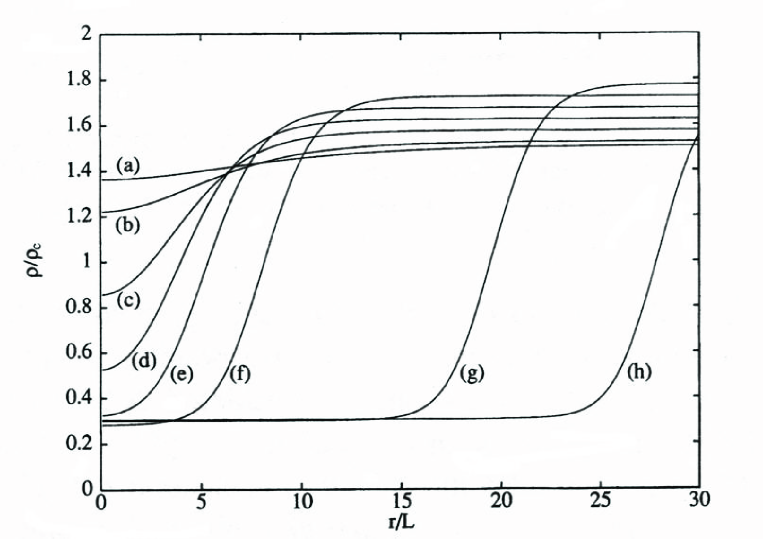
Figure 1: Density profiles for van der Waals equations of state for different values of $\mu_{\infty}$ (or $\rho_{\infty}$) at $t=0.85$ obtained by numerical solution of the DPE. Towards saturation, cf. the curves labeled from (e) to (h), the bubble clearly develops a bulk vapor phase in its interior. Near the minimal nucleation radius, cf. the curve (d), the bulk vapor phase disappears. In the spinoidal limit, cf. the curves from (c) to (a), the radius of the bubble again grows but no bulk vapor phase exists and the density jump rapidly decreases until it disappears at the so-called spinoidal composition in which only the liquid phase exists.

Typical density profiles are shown in Figure 1 for the van der Waals equation of state. The two parts of the nucleation phenomenon, i.e., the homogeneous nucleation and the growth of bubble approaching saturation, are clearly seen in this figure. The density profile tends to be diffuse towards the spinoidal limit so that the density jump $\rho_{\infty}-\rho(0)$ goes to zero (cf. curves (a), (b) and (c) in Figure 1). Approaching saturation, a region of almost-constant density appears before the phase transition region, i.e. a bulk vapor phase, and the density jump is practically constant (cf. curves (f), (g) and (h) in Figure 1).

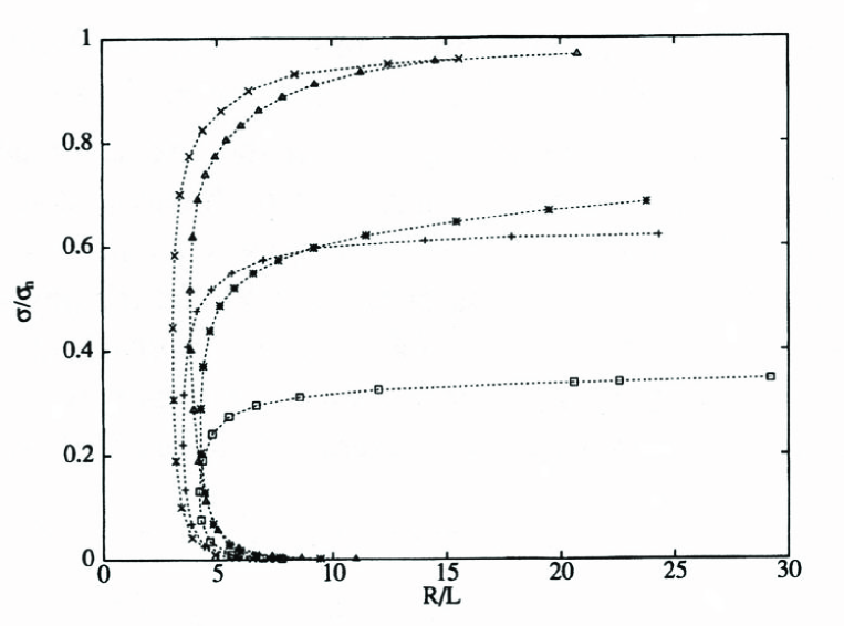
Figure 2: Normalized surface tension $\sigma/\sigma_{n}$ where $\sigma_{n}=\rho_{c}R_{\mathcal{M}}T_{c}\mathcal{L}$ vs normalized equilibrium radius $R/\mathcal{L}$ of microscopic bubbles at $t=0.85$ for the following equations of state: van der Waals $\Box$; Rocard 4 $\star$; Berthelot $\times$; Peng-Robinson $\triangle$; Eberhart-Schnyders $+$. The end-point of each curve toward the saturation have to be considered equivalent in the sense of saturation proximity (cf. the text).

In Figure 2 we show the dependence of $\sigma$ on $R$ (as defined in Section 3.4) numerically evaluated at the reduced temperature $t=0.85$ for some of the equations of state listed in Table 1. The results are qualitatively similar: for small values of $\mu_{\infty}$ near the spinoidal value $\mu_{\infty}^{bub,spi}$ (i.e. the lower part of the curve in Figure 2), $\sigma$ initially vanishingly small, grows slowly whereas the radius decreases towards a minimal value that we identify as the ’minimal nucleation radius’ $R_{m}$. At $R_{m}$ the surface tension suddenly increases and the density at the center of the bubble reaches the range of the vapor phase (cf. also curves (d) and (e) in Figure 1). Above the minimal nucleation radius, $\sigma$ approaches within a few minimal radii the planar interface value and, as shown by Fisher and Israelachivli experiments, remains substantially constant [18]. We note that quantitatively, the van der Waals equation of state gives the lowest value of planar interface surface tension, the Berthelot and the Peng-Robinson give the highest values. The behavior for other values of temperature is qualitatively the same. We note also that the curves end at different radii as they approach saturation; these radii have to be considered as equivalent because the ’distance’ from saturation, measured by the difference between the first maximum of the potential and the density at the center of the bubble, is in all cases less than $10^{-16}$. It could be implied by this circumstance that different equations of state reach saturation at different radii. Moreover we note that curves corresponding to radii between the spinoidal and the minimal critical radius values can be considered as lacking physical meaning because, no physical bubble can exist in this regime, except fluctuations of typical radius $R$ (cf. [3]). So the ’minimal nucleation radius’ $R_{m}$ marks the last values, before the spinoidal, to which one can give physical meaning.
In Figure 3 we plot the (equivalent) interface thickness defined in Eq. (3.20) as a function of $R$ for some of the different equations of state, always at reduced temperature $t=0.85$. At the start of nucleation (spinoidal limit), $\delta$ is very large (diffuse interface) and of the same order of magnitude as $R$: density fluctuations have a unique length scale. When $R$ has reached the minimal nucleation radius, $\delta$ quickly tends to a practically constant value with very small deviation from the limit value at saturation. Again all the studied equations of state have the same qualitative behavior. Moreover, we note that the curves between the spinoidal limit and the minimum radius are essentially the same for all the equations of state used here (cf. Figure 3).
We note that no qualitative differences appear when the temperature is changed. It is also interesting to note that the ratio $(\delta/R)_{m}$ is, within the numerical accuracy, a constant independent of $t$: its value is reported in Table 2 for all equations of state. Moreover this constant is practically the same for all the equations of state studied here, i.e., $(\delta/R)_{m}\sim\;0.42-0.44$. The justification of this phenomenon can be that, the shell-like quantities as surface tension, radius, etc., being defined through an integral over the thickness of the interface, the differences between the equations of state will be smeared by integration, giving similar results.

State Equation	$(\delta/R)_{m}$	$\delta_{\infty}/\delta_{m}$	$\rho_{\sigma}^{\infty}/\rho_{\sigma}^{m}$
van der Waals	$0.427$	$0.771$	$0.716$
Rocard 1	$0.443$	$0.778$	$0.712$
Rocard 2	$0.435$	$0.785$	$0.739$
Rocard 3	$0.443$	$0.768$	$0.716$
Rocard 4	$0.432$	$0.795$	$0.773$
Berthelot	$0.426$	$0.768$	$0.710$
Eberhart-Schnyders	$0.428$	$0.761$	$0.683$
Peng-Robinson	$0.439$	$0.750$	$0.767$

Table 2.  Numerically evaluated ratios $(\delta/R)_{m}$, $\delta_{\infty}/\delta_{m}$ and $\rho_{\sigma}^{\infty}/\rho_{\sigma}^{m}$ for the equations of state reported in Table 1. The ratios are substantially independent of the temperature in the limit of the algorithm error introduced in the numerical solutions of the DPE equation.

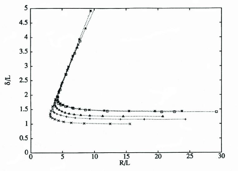
Figure 3: Normalized thickness $\delta/\mathcal{L}$ of the interface vs normalized equilibrium radius $R/\mathcal{L}$ of microscopic bubbles at $t=0.85$ for the following equations of state: van der Waals $\Box$; Rocard 4 $\star$;Berthelot $\times$; Peng-Robinson $\triangle$; Eberhart-Schnyders $+$.

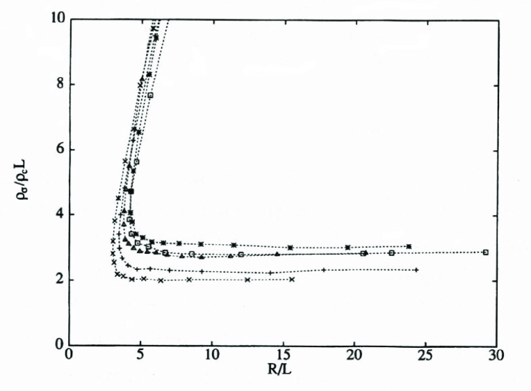
Figure 4: Normalized surface mass density $\rho_{\sigma}/(\rho_{c}\mathcal{L})$ vs normalized equilibrium radius $R/\mathcal{L}$ of microscopic bubbles at $t=0.85$ for the following equations of state: van der Waals $\Box$; Rocard 4 $\star$; Berthelot $\times$; Peng-Robinson $\triangle$; Eberhart-Schnyders $+$.

In Figure 4 we plot the surface mass density versus $R$ at $t=0.85$ obtained by using Eq. (3.22) for the same equations of state than in Figures 2-3. We see that surface mass is an increasing function of $R$ going towards the spinoidal limit. This behavior is obviously due to the increase of $\delta$ in the same limit. Again we note that no qualitative differences appear when the temperature is changed. Moreover the ratios $\delta_{\infty}/\delta_{m}$ and $\rho_{\sigma}^{\infty}/\rho_{\sigma}^{m}$ are independent of $t$. Their values, listed in Table 2 for all the equations of state, differ by less than $15\%$.

5 Minimal nucleation radii: theoretical predictions and comparison with experiments

The comparison of the above results with the experimental values reported in literature is a rather difficult task because information for many data can be only indirectly recovered. Moreover, as shown in Section 4.2, Eqs (4.5-4.7), all the predictions are critically dependent on the parameters of the intermolecular potential; in our case a fundamental role is played by $\mathcal{L}$ that sets the length scales. Again the correct prediction of surface tension is also not simple in the sophisticated microscopic statistical theories (cf. the data reported in [16]) because, especially at very small scales, the details of the intermolecular potential, and so the particular molecular micro-structure, are relevant in the determination of the exact values of surface tension. We prove in this paper that rather good predictions of surface tension are also possible in the framework of the second gradient theory.

Moreover we are able to produce predictions of nucleation radius. In particular, by evaluating $R_{m}$, we establish a lower bound to the experimental nucleation radii reported in the literature. We remark that very few data are found in the literature concerning bubbles (cf. [41]), so that we are obliged to compare these predictions with data for the droplets found in Lamer and Pound or Kumar [28, 29].
In order to choose, for every substance, the most suitable equations of state to predict the minimal nucleation radius, we use the planar interface surface tension values in the following way: by following Cahn and Hilliard, we fix $\mathcal{L}$ (cf. the next subsection) while among the considered equations of state, we choose that which predicts $\sigma_{\infty}$ values sufficiently accurately (for many substances this estimate holds within $90\%$ of the experimental value). Finally we can predict the thickness of the interface and the surface mass density. We note that these data are relatively scarce especially the latter [1, 11].

5.1 The planar interface surface tension.

Substance	$t_{exp}$	$\sigma^{exp}_{\infty}\;\;\;[\frac{dyn}{cm}]$	$\sigma^{vdw}_{\infty}\;\;\;[\frac{dyn}{cm}]$	$\alpha_{exp}$
Ar	$\sim 0.5$	$13.1$	$23.9$	$3.24$
CO2	$0.95$	$1.16$	$0.93$	$1.51$
N2	$\sim 0.6$	$9.80$	$8.25$	$1.50$
O2	$\sim 0.6$	$13.2$	$11.4$	$1.46$
H2	$\sim 0.6$	$2.09$	$2.29$	$1.34$
H2O	$0.5$	$68.5$	$63.8$	$1.83$
NH${}_{3}^{*}$	$\sim 0.7$	$23.4$	$26.3$	$1.73$
CH3OH	$\sim 0.6$	$20.1$	$20.1$	$1.91$
C2H5OH∗	$\sim 0.5$	$22.7$	$24.7$	$1.70$
C2H${}_{6}^{*}$	$\sim 0.6$	$16.2$	$15.3$	$1.50$
C6H12	$0.5$	$25.5$	$16.5$	$1.63$
CCl4	$\sim 0.5$	$29.8$	$18.6$	$1.64$
CF4	$\sim 0.9$	$5.0$	$0.87$	$-$

Table 3. Planar interface surface tension for some substances evaluated in the case of van der Waals equation of state and the corresponding experimental value. In the last column of the Table is reported the scaled parameter $\displaystyle\alpha_{exp}=\frac{a_{exp}\rho_{c}}{\mathcal{M}RT_{c}}$. For experimental planar interface surface tension cf. [19, 26]. The upper part of the Table shows substances for which Lennard-Jones radius $r$${}_{{\small{}_{LJ}}}$ is known with good approximation and so it is used to calculate $\sigma_{\infty}$ by evaluating $\mathcal{L}$ from $\displaystyle(11/7)^{\frac{1}{2}}r$${}_{{\small{}_{LJ}}}$. In the lower part of the Table (down the double line) the covolume radius $r_{co}$ is used to evaluate $\mathcal{L}$ and then $\sigma_{\infty}$. In the cases marked by ^∗ a better fitting was made by taking $\mathcal{L}=1.25\;r_{co}$.

In Table 3 we show collected experimental data for different substances. Values for the planar interface surface tension are shown together with the values evaluated by second gradient theory in the case of the van der Waals equation of state. The theoretical predictions were made by using in some cases the Lennard-Jones relation between $r_{0}\equiv r_{{}_{LJ}}$ and $\mathcal{L}$ while in others we have simply put $\mathcal{L}=r_{0}=r_{co}$, where $r_{co}$ is the covolume radius (we note that in general $r_{{}_{LJ}}>r_{co}$ but their ratio is lower than $(11/7)^{\frac{1}{2}}\sim 1.25$).

The prediction of the second gradient theory is generally within $20\%$ of the experimental value: this can be considered as a good result, comparable with the non-local model approach (cf. [8] and [16]). In many cases our predictions are very accurate. We note however that are remarkable exceptions: 1) the Ar value is larger by about a factor two with respect to the experimental value; the same holds true in respect of the surface tension for other noble gases; 2) the values for C₆H₁₂ and CCl₄ are smaller almost by a factor of two (about $60\%$ of experimental values), the same is true in minor form also for other carbon compounds such as C₄H₁₀ and C₃H₈ and most dramatically for CF₄, where the ratio is about $1/6$.

The case of Argon and the other noble gases can be understood if we look to the last column of Table 3 in which we report the scaled experimental value of $\displaystyle\alpha_{exp}=\frac{a_{exp}\rho_{c}}{\mathcal{M}RT_{c}}$ representing the normalized value of the van der Waals constant $a$. For all substances $\alpha_{exp}$ is between $1$ and $2$ whereas for Ar it is larger than $2$ (about $3.2$); the same is true for other noble gases. This large value implies that the values of surface tension evaluated with the ’van der Waals theory’ are generally far from the experimental values. This is a known result for Ar [16]: the second gradient theory is insufficient to reproduce the experimental value for the surface tension, as higher-order gradients are necessary in the constitutive law for free energy to give a correct prediction (cf. [15]).

As for point 2) we could increase the values of the surface tension, by multiplying $r_{co}$ by $1.25$, i.e., the Lennard-Jones factor. This trick works effectively for ethyl alcohol, ethane and ammonia, but for the other substances the theoretical surface tension remains too small when compared with the experimental value (we note also the case of CO₂ in which the theoretical value is $79\%$ of the experimental value). So we conjecture that other equations of state, that generally have a larger value of $\sigma_{\infty}$ (cf. Fig. 2), would describe carbon compounds better than the van der Waals equation. For the sake of brevity we do not present the theoretical data; we limit ourselves to saying that, by using a different equation of state, the values of $\sigma_{\infty}$ can be predicted with the same precision as shown in Table 3 for substances that are well described by the van der Waals equation.

5.2 The minimal nucleation radius and the other surface quantities

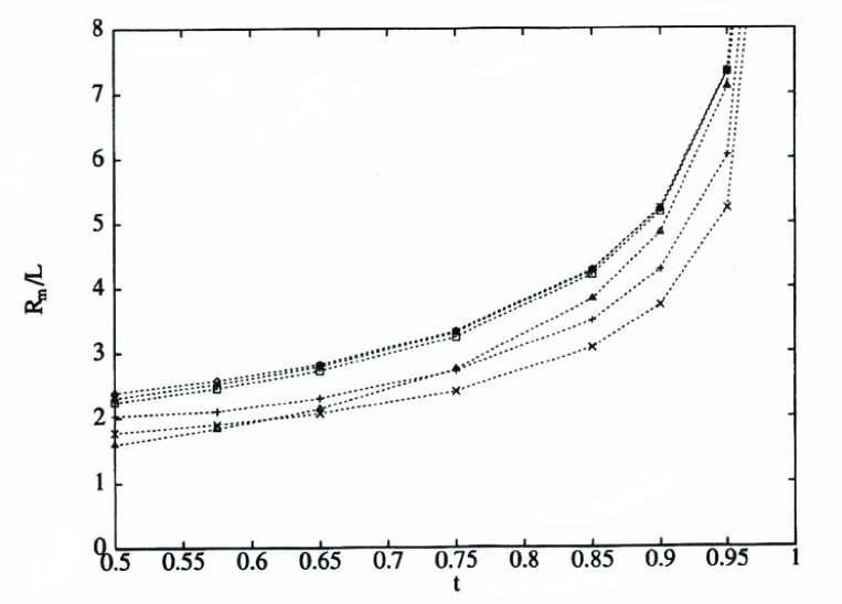
Figure 5: Minimal nucleation radii vs reduced temperature in units of $\mathcal{L}$ in the interval $[0.5,1.0[$ for the following equations of state: van der Waals $\Box$; Rocard 3 $\Diamond$; Rocard 4 $\star$; Berthelot $\times$; Peng-Robinson $\triangle$; Eberhart-Schnyders $+$. State equations Rocard 1 and 2 give minimal nucleation radii between Rocard 3 and van der Waals cases.

In Figure 5 we display the normalized minimal nucleation radius in units of $\mathcal{L}$ for the equations of state in Table 1 versus reduced temperature in the interval $[0.5,1.0[$. The interval chosen is the most relevant for many substances because most of the experimental data on surface tension exist in this range of reduced temperature (cf. [19, 26]). At the lower temperatures the minimal radius tends to be a constant of approximate value $\mathcal{L}$; the exact values could be retrieved in principle by the method described in Section 4, but the strong stiffness of the problem, induced by the rapid decrease to very small values of the gas phase density, limits the precision of the method.

Substance	$R_{m}$ [Å]	$\delta_{m}$ [Å]	$\rho_{\sigma}^{m}\;10^{-7}\cdot[g/cm^{2}]$
CO2	$22.3$	$9.52$	$9.4$
N2	$19.7$	$8.47$	$5.7$
O2	$18.4$	$7.86$	$7.4$
H2	$15.6$	$6.67$	$0.4$
H2O	$15.5$	$6.63$	$4.6$
NH${}_{3}^{*}$	$20.8$	$8.87$	$4.5$
CH3OH	$20.2$	$8.62$	$5.0$
C2H5OH∗	$27.3$	$11.6$	$6.9$
C2H${}_{6}^{*}$	$24.9$	$10.6$	$4.7$

Table 4. Minimal nucleation radii for bubbles of some substances evaluated at $t=0.85$ in the case of van der Waals equation of state. In the other two columns are listed the predicted values of thickness and surface mass density at minimal nucleation radius at the same reduced temperature. The meaning of the division of the Table in upper and lower part and the ^∗ near some substance is the same than in Table 3.

We see that the Berthelot equation of state and the modification proposed by Eberhart-Schnyders [41] predict radii rather smaller than other equations of state. The Peng-Robinson equation of state gives radii near to the van der Waals model at high values of $t$ and near the Berthelot model values at about $t=0.5$. The family of all equations of state proposed by Rocard give radii very near to the van der Waals value (for this reason only two of these data are reported in Figure 5, in order to leave the figure sufficiently clear). Obviously, when the critical temperature is approached the minimal radius and the thickness tend to $\infty$.

Substance	State Equation	$R_{m}$ [Å]	$\delta_{m}$ [Å]	$\rho_{\sigma}^{m}\;10^{-7}\cdot[g/cm^{2}]$
CH4	Eberhart-Schnyders	$13.1$	$5.70$	$2.0$
C3H8	Rocard 4	$22.1$	$9.54$	$4.6$
C3H8	Eberhart-Schnyders	$18.1$	$7.86$	$3.8$
C4H10	Rocard 4	$25.1$	$10.8$	$5.4$
C4H10	Eberhart-Schnyders	$20.5$	$8.90$	$4.5$
C6H12	Rocard 4	$26.3$	$11.3$	$6.8$
C6H12	Peng-Robinson	$23.6$	$10.2$	$6.2$
CCl4	Rocard 4	$26.1$	$11.2$	$13.8$
CCl4	Peng-Robinson	$23.4$	$10.1$	$12.6$

Table 5.  Minimal nucleation radii for bubbles of some substances (carbon compounds) evaluated at $t=0.85$ in the case of some other equations of state. These will be chosen to reproduce the planar interface surface tension experimental values at least to $80\%$. In the other two columns are listed the predictions for thickness and surface mass density at minimal nucleation radius at the same reduced temperature.

In Table 4, the minimal nucleation radii at $t=0.85$ are listed for those substances whose planar interface surface tension is well described by the van der Waals equation of state. In the same table, we have added data on the thickness of the interface and the surface mass density for the substances cited therein. In Table 5, further theoretical predictions are given, always at $t=0.85$, for substances whose planar interface surface tension is well described by other equations of state. Thus we show that radii, thickness and surface mass densities can be calculated very easily by using the results found in [13]. We note that the minimal radius ranges typically from $10$ to $30$ Å  so that it is just a few molecular radii. For example the molecules of C₆H₁₂ have a radius of about $5$ Å; at $t=0.85$ the ratio between this value and predicted minimal radius is about $4.7$, while at $t=0.5$ the minimal nucleation radius is $\sim 9.8$ Å  and the ratio is about $2$.

Examples of predictions of the equilibrium radius as a function of $R$ (or $\mu_{\infty}$) by means of classical theory are given by van Carey [41]. However he limits himself to the case of ’large bubbles’, the only ones for which classical theory is valid. The experiment of Fisher and Israelachvili [18] needs to be reinterpreted because the Laplace formula, on which is based the Kelvin relation used to extrapolate the radius, is not valid near the minimal nucleation radius [12]. Moreover, as noted above, their results can be compared with a process of homogeneous nucleation only after a thorough analysis of the effect of their experimental apparatus. We note that as cited above C₆H₁₂ has a predicted minimal nucleation radius of about $\sim 9.8$ Å at the temperature in which the experiment was performed ($t\sim 0.5$). It is larger than the radii reported by Fisher and Israelachvili (we also note that, on changing the equations of state or the evaluation of $\mathcal{L}$, the minimal radius always remains greater than their data). On the other hand, data on homogeneous nucleation for very small radii exist for droplets (cf. [28, 29]) and comparison with our data shows that the nucleation radii of bubbles we predict are in some cases very close to nucleation radius for the droplets; for example, in the case of water, the Lamer and Pound data are in the range $8.0-8.9$ Å at $t\sim 0.5$, and our prediction is $R_{m}\simeq 8.3$ Å; the data for equilibrium radii reported by Kumar for the CCl₄ at $t\simeq 0.5$ range between $12-17$ Å, these are very close to those we calculated which range (at $t=0.5$) between $12-14$ Å, though this range of variation is due to the used equation of state rather than to the supersaturation ratio.

Moreover we predict that the thickness of the interface is formed by few molecular layers [16] in the range from minimal nucleation radius to saturation. A new insight of the physical problem is obtained when observing that at small radii the interface constitutes a large part of the microscopic bubbles and cannot be confined in any Gibbs-Tolman idealized zero thickness layer. Typically the numerically evaluated ratio between the equivalent thickness at the minimal radius and the minimal radius itself is of the order of $0.4$ for all the equations of state studied here. Finally we note that the surface mass density values (see Tables 4 and 5) are of the order of magnitude predicted by Alts and Hutter in their theory on water [1].

6 Conclusion

The first three Sections of this paper give a complete account of the results available in the literature concerning the theoretical treatment of the phenomenon of homogeneous nucleation and the dependence of surface tension on curvature.

However recently (cf. [12]) a rational definition for surface tension and radius of curvature for spherical interfaces has been proposed in terms of a solution of the density field, using a shell-like approach to the definition of interface quantities. Moreover, thanks to the second gradient theory, a deeper understanding of the relationship between the Laplace formula and the capillary constant $\lambda$ has become possible. In particular our investigations stem from a theoretical treatment in which:
1) an expression for surface tension is used which accounts for curvature effects better than those found in the literature;
2) the mechanical pressure is distinguished from the thermodynamic pressure.

In this way we obtained, using numerical methods, predictions for:
1) the dependence of surface tension, equilibrium radius, thickness of the spherical interface and surface mass density on chemical potential;
2) the values of the minimal nucleation radius, i.e., the minimum equilibrium radius possible for a bubble. Being founded either on statistical mechanics or on second gradient theories, our predictions have a clear meaning in a range of temperature close to the critical point.

Possible generalizations include the study of:
(i) models in which $\lambda$ depends on $\rho$ locally or globally;
(ii) models in which higher density gradients appear, or a fully non-local approach via integral equations;
(iii) models suitable to describe the dynamics of phase transitions.

Acknowledgements:

We wish to thank A. Di Carlo, P. Seppecher and W. Kosiński for their friendly criticism. This work was financially supported by the Université de Toulon et du Var, the Université of Aix-Marseille and the Italian CNR.

References

- [1] Alts T., Hutter K., 1988, Continuum description of the dynamics and thermodynamics of phase boundaries between ice and water. Parts I and II, J. of Noneq. Therm., 13, 221-280.
- [2] Blinowski A., 1974, Mathematical theory of Spherical interfaces, Arch. Mech., 26, 953-975.
- [3] Cahn J.W., Hilliard J.E., 1958, Free energy of a non-uniform system I, J. Chem. Phys. 28, p.258-267; Cahn J.W., Hilliard J.E., 1959, Free energy of a non-uniform system III, J. Chem. Phys. 31, 688-699.
- [4] Casal P., 1961, La capillarité interne, Cahier du groupe Francais de rhéologie, CNRS VI, 3, 31-37.
- [5] Casal P., 1972, La théorie du second gradient et la capillarité, C. R. Acad. Sci. Paris, 274, Série A, 1571-1574.
- [6] Casal P., Gouin H., 1985, Relation entre l’équation de l’énergie et l’équation du mouvement en théorie de Korteweg de la capillarité, C. R. Acad. Sci. Paris, 300, Série II, 231-234.
- [7] Chattoraj D.K., Birdi K.S., 1984, Adsorption and the Gibbs surface excess, Plenum, New York.
- [8] Davis H., Scriven L., 1982, Stress and Structure in fluid interfaces, Adv. Chem. Phys., 49, 357-454.
- [9] de Gennes P.G., 1981, Some effects of long range forces on interfacial phenomena, J. Physique-Lettres 42, L-377, L-379.
- [10] Dell’Isola F., Kosiński W., 1993, Deduction of thermodynamics balance laws for bidimensional nonmaterial directed continua modelling interphase layers, Arch. Mech., 45, 333-359.
- [11] Dell’Isola F., 1994, On the lack of structure of 2D Defay-Prigogine continua, Arch. Mech., 46, 329-341.
- [12] Dell’Isola F., Rotoli G., 1994, On the generalization of Tolman formula, Atti XII Congresso Nazionale Trasmissione del Calore, 327-338.
- [13] Dell’Isola F., Gouin H., Seppecher P., 1995, Radius and surface tension of microscopic bubbles by second gradient theory, C. R. Acad. Sci. Paris, 320, II, 211-217.
- [14] Dunn J.E., Serrin J., 1985, On the thermodynamics of interstitial working, Arch. Rat. Mech. Anal., 88, 95-133.
- [15] Ebner C., Saam W.F., Stroud D., 1976, Density-functional theory of simple classical fluids. I, Surfaces, Phys. Rev. A, 14, 2264-2273.
- [16] Evans R., 1979, The nature of the liquid-vapor interface and other topics in the statistical mechanics of non-uniform classical fluids, Adv. in Phys., 28, 143-200.
- [17] Falls A., Scriven L., Davis H., 1981, Structure and stress in spherical microstructures, J. Chem. Phys., 75, 3986-4002.
- [18] Fisher L.R., Israelachvili J.N., 1980, Determination of the capillary pressure in menisci of molecular dimensions, Chem. Phys. Letters, 76, 325-328.
- [19] Gaz Encyclopedia, 1976, L’air Liquide, Amsterdam.
- [20] Germain P., 1972, La méthode des puissances virtuelles en mécanique des milieux continus - Théorie du second gradient, J. de Mécanique, 12, 235-274.
- [21] Gibbs J.W., 1948, Collected works, vol. 1, Yale Univ. Press.
- [22] Gouin H., 1987, Equation du mouvement des fluides parfaits de grade n exprimée sous une forme thermodynamique, C. R. Acad. Sci. Paris, 305, Série II, 833-838.
- [23] Gouin H., 1988, Une interprétation moléculaire des fluides thermocapillaires, C. R. Acad. Sci. Paris, 306, Série II, 755-759.
- [24] Gouin H., Slemrod M., 1995, Stability of spherical isothermal liquid-vapor interfaces, Meccanica, 30, 305-319.
- [25] Gurtin M.E., 1965, Thermodynamics and the possibility of spatial interaction in elastic materials, Arch. Rat. Mech. Anal., 19, 339-352.
- [26] Handbook of Chemistry and Physics, 1992, 73th edition, CRC, Boca Raton, Florida, (6-126)-(6-130).
- [27] Korteweg D.J., 1901, Sur la forme que prennent les équations du mouvement des fluides si l’on tient compte des forces capillaires…, Arch. Néerl. Sci. Ex. Nat. Série II, 6, 1-24.
- [28] Kumar F.J., Jayaraman D., Subramanian C., Ramasamy P., 1991, Curvature dependence of surface free energy and nucleation kinetics of CCl4 and C2H2Cl4 vapours, J. of Material Sci. Lett., 10, 608-610.
- [29] Lamer V.K., Pound G.M., 1949, Surface tension of small droplets from Volmer and Flood’s nucleation data, Chem. Phys. Lett. 17, 1337-1338.
- [30] Peletier L., Serrin J., 1986, Uniqueness of non-negative solutions of semilinear equations, J. Diff. Eq., 61, 380-397.
- [31] Peng D.Y., Robinson D.B., 1976, A new two-constant equation of state, Ind. Eng. Chem. Fundam., 15, 59-64.
- [32] Percus J.K., Yevik G., 1958, Analysis of classical statistical mechanics by means of collective coordinates, Phys. Rev., 110, 1.
- [33] Press W.H. et al., 1986, Numerical recipes, Cambridge Univ. Press, Cambridge, chap. 16, 718-725.
- [34] Rocard Y., 1967, Thermodynamique, Masson, Paris, chap. V.
- [35] Seppecher P., 1987, Etude d’une modélisation des zones capillaires fluides; interfaces et ligne de contact, Thèse, Université Paris VI and E.N.S.T.A..
- [36] Serrin J., 1959, Mathematical principles of classical fluid mechanics, Encyclopedia of Physics, S. Flügge Ed., vol.VIII/1, Springer, Berlin, 125-263.
- [37] Serrin J., 1986, New perspectives in thermodynamics, Springer, Berlin, 187-260.
- [38] Tolman R.C., 1948, Consideration of the Gibbs theory of surface tension, J. Chem. Phys. 16, 758-774.
- [39] Tolman R.C., 1949, The effects of droplet size on surface tension, J. Chem. Phys. 17, 333-337.
- [40] Truskinovsky L., 1983, Critical nuclei in the van der Waals model, Sov. Phys. Dokl., 28, 3, 248-250.
- [41] van Carey P., 1993, Liquid-vapor phase-change phenomena, Hemisphere, Washington, chap. 5, 127-167.
- [42] van Kampen N.G., 1964, Condensation of a classical gas with long range attraction, Phys. Rev., 135, A362-A369.