Money Distributions in Chaotic Economies

Abstract

This paper considers the ideal gas-like model of trading markets, where each individual is identified as a gas molecule that interacts with others trading in elastic or money-conservative collisions. Traditionally this model introduces different rules of random selection and exchange between pair agents. Real economic transactions are complex but obviously non-random. Consequently, unlike this traditional model, this work implements chaotic elements in the evolution of an economic system. In particular, we use a chaotic signal that breaks the natural pairing symmetry $(i,j)\Leftrightarrow(j,i)$ of a random gas-like model. As a result of that, it is found that a chaotic market like this can reproduce the referenced wealth distributions observed in real economies (the Gamma, Exponential and Pareto distributions).

Keywords: Econophysics, Gas-like Models, Complex Systems, Chaos, Nonlinear Maps.

I Introduction

Econophysics is a relatively new discipline  [1] that applies many-body techniques developed in statistical mechanics to the understanding of self-organizing economic systems  [2]. The techniques used in this field  [3],  [4],  [5] have to do with agent-based models and simulations. The statistical distributions of money, wealth and income are obtained on a community of agents under some rules of trade and after an asymptotically high number of interactions between the agents.

The conjecture of a kinetic theory with (ideal) gas-like behaviour for trading markets was first discussed in 1995  [6] by econophysicists. This model considers a closed economic community of individuals where each agent is identified as a gas molecule that interacts randomly with others, trading in elastic or money-conservative collisions. Randomness is an essential ingredient in this model, where agents interact in pairs chosen at random by exchanging a random quantity of money. The interesting point of this model is that, by analog with Energy, the equilibrium probability distribution of money follows the exponential Boltzmann-Gibbs law for a wide variety of trading rules  [2].

This result is coherent with real economic data up to some extent. Nowadays it is well established that the income and wealth distributions in many countries follow a characteristic pattern. They seem to present two phases with different richness distributions. One phase presents an exponential (Boltzmann-Gibbs) distribution and covers about $90-95\%$ of individuals, those with low and medium incomes. The other phase, which is integrated by the rest of the individuals with high incomes, shows a power law (Pareto). This is so in different countries, irrespective of their differences in cultural or social structures ,  [7],  [8], from older societies  [9]  [10]  [11]  [12] to modern ones  [13],  [14],  [15].

This paper introduces chaotic-driven dynamics in the economic gas-like model. The objective is obtaining money distributions similar to those observed in real economies. This is a novel approach, where the rules of selection of agents and money transfers are no longer random, but driven by nonlinear maps in chaotic regime. Two different scenarios are considered and the money distributions, obtained that way, are compared to the distributions shown in real economies.

The contents of this paper are organized as follows: section 2 describes the simulation scenario. Section 3 show the results obtained. Final conclusions are in Section 4.

II Scenario of Chaotic Simulation

This paper introduces chaos in the dynamics of the economic gas-like model. This is done upon two facts that seem particularly relevant in this purpose.

The first one is, that real Economy is not purely random. Economic transactions are driven by some specific interest (of profit) between the interacting parts. Thus, on one hand, there is some evidence of markets being not purely random. On the other hand, everyday life shows us the unpredictable component of real economy with its recurrent crisis. Hence, it can be sustained that the short-time dynamics of economic systems evolves under deterministic forces though, in the long term, these kind of systems show an inherent instability. Therefore, the prediction of the future situation of an economic system resembles some-how to the weather prediction. It can be concluded that determinism and unpredictability, the two essential components of chaotic systems, take part in the evolution of Economy and Financial Markets.

The second fact is, that the transition from the Boltzmann-Gibbs to the Pareto distribution can require the introduction of some kind of inhomogeneity that breaks the random indistinguishability among the individuals in the market, although this is not a necessary condition in order to have such kind of transition [16]. Nonlinear maps can be an ideal candidate to obtain that, as they can offer quite flexible models of evolution in the market. In particular, nonlinear maps can be easily tuned to break the pairing symmetry of agents $(i,j)\Leftrightarrow(j,i)$, characteristic of the random model.

The simulation scenario presented here follows a traditional gas-like model. A community of $N$ agents is given with an initial equal quantity of money, $m_{0}$, for each agent. The total amount of money, $M=N*m_{0}$, is conserved in time. For each transaction, a pair of agents $(i,j)$ is selected, and an amount of money $\Delta m$ is transferred from one to the other. In this work two simple and well known rules are used. Both consider a variable $\upsilon$ in the interval $(0,1)$, not necessarily random, in the following way:

• Rule 1: the agents undergo an exchange of money, in a way that agent $i$ ends up with a $\upsilon$-dependent portion of the total of two agents money, ($\upsilon*(m_{i}+m_{j})$), and agent $j$ takes the rest ($(1-\upsilon)*(m_{i}+m_{j})$)  [17].

• Rule 2: an $\upsilon$-dependent portion of the average amount of the two agents money, $\Delta m=\upsilon*(m_{i}+m_{j})/2$, is taken from $i$ and given to $j$  [3]. If $i$ doesn’t have enough money, the transfer doesn’t take place.

As there are two different simulation parameters involved in these gas-like models (the parameter for selecting the agents involved in the exchanges and the parameter defining the economic transactions), two different scenarios are obtained depending on the random-like or chaotic election of these parameters. These scenarios are the following:

• Scenario I: random selection of agents with chaotic money exchanges.

• Scenario II: chaotic selection of agents with random money exchanges.

To produce chaotically a pair of agents $(i,j)$ for each interaction, a 2D nonlinear map under chaotic regime is considered. The pair $(i,j)$ is easily obtained from the coordinates of a chaotic point at instant $t$, $X_{t}=[x_{t},y_{t}]$, by a simple float to integer conversion ($x_{t}$ and $y_{t}$ to $i$ and $j$, respectively). Additionally, to obtain a chaotic money exchange, a float number $\upsilon$ in the interval $[0,1]$ is obtained form the coordinates of a chaotic point at instant $t$ by taking one or a combination of both. This number produces the chaotic quantity of money $\Delta m$ that is traded between agents $i$ and $j$.

The simulation scenario uses two particular 2D nonlinear maps under chaotic regime. These are the Henon map described in  [18] (1) and the Logistic bimap described in  [19] as model (a) (2) . These maps are given by the following equations:

$$\begin{array}[]{l}T_{H}:\Re\times\Re\longrightarrow\Re\times\Re\\ x_{t+1}=ax_{t}^{2}+y_{t}+1,\\ y_{t+1}=bx_{t}.\end{array}$$ (1)

$$\begin{array}[]{l}T_{A}:[0,1]\times[0,1]\longrightarrow[0,1]\times[0,1]\\ x_{t+1}=\lambda(3y_{t}+1)x_{t}(1-x_{t}),\\ y_{t+1}=\lambda(3x_{t}+1)y_{t}(1-y_{t}).\end{array}$$ (2)

These maps show chaotic behaviour for some values of their parameters. In this work the following values are considered: the Hénon map in its canonical with $a=1.4$ and $b=0.3$ and the Logistic bimap when $\lambda_{a}$ and $\lambda_{b}$ are in the interval $[1.032,1.0843]$, where chaotic regime can be obtained.

To conclude the description of the simulation scenario, it is interesting to point out here that the two rules of trade considered here exhibit different symmetry of exchange. Rule $2$ is asymmetric for it takes money from $i$ agent and gives it to the other. When considering the chaotic maps, the Henon map is asymmetric and the Logistic bimap exhibits symmetric behaviour along the diagonal axis (straight line $y=x$) when $\lambda_{a}$=$\lambda_{b}$. This symmetry is modified in the simulations to show how asymmetry can affect the final money distributions.

III Asymptotic Money Distributions

The (ideal) gas-like model, as described in the precedent sections shows an equilibrium distribution of money that follows the exponential Boltzmann-Gibbs law for a wide variety of trading rules  [2, 20].

In this section, chaos is introduced in this model. Different scenarios are presented depending on the way this chaoticity is established. These scenarios where first proposed by the authors in  [21]. The obtained asymptotic money distributions are presented, compared to the exponential and discussed in order to provide illuminating ideas about the cause of these particular results.

III-A Scenario I: random agents/chaotic trade

In this scenario, the selection of agents is random as in the traditional gas-like model. Individuals don’t have preferences in choosing an interaction partner, commercial transactions are nor restricted, nor driven by particular interests. But unlike this model, the exchange of money is forced to evolve according to nonlinear patterns. Economically, this means that the exchange of money has a deterministic component, although it varies chaotically. Put it in another way, the prices of products and services are discrete and evolve in a limited range, in a complex way.

A community of $N=500$ individuals is considered with an initial quantity of money of $m_{0}=1000\$$. This community takes a total time of $400000$ transactions. For each transaction two random numbers from a standard random generator are used to select a pair of agents. Additionally, a chaotic float number is produced to obtain the float number $\upsilon$ in the interval $[0,1]$. The value of $\upsilon$ is calculated as $|x_{i}|/1.5$ for the Hénon map and as $x_{i}$ for the Logistic bimap. This value and the rule selected for the exchange determine the amount of money $\Delta m$ that is transferred from one agent to the other.

Different cases are considered, taking the Hénon chaotic map or the Logistic bimap. Rules 1 and 2 are also considered. New features appear in this scenario. These can be observed in Fig.1 and Fig.2.

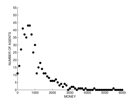
Figure 1: Chaotic trade selection with Logistic Bimap and Rule 1

Figure 2: Chaotic trade selection with Logistic Bimap and Rule 2

The first feature is that the chaotic behavior of $\upsilon$ is producing a different final distribution for each rule. Rule 2 is still displaying the exponential shape, but Rule 1 gives a different asymptotic function distribution, it becomes a Gamma-like distribution. It presents a very low proportion of the population in the state of poorness, and a high percentage of it in the middle of the richness scale, near to the value of the mean wealth. Rule 1 seems to lead to a more equitable distribution of wealth.

Basically, this is due to the fact that Rule 2 is asymmetric. Each transaction of Rule 2 represents an agent $i$ trying to buy a product to agent $j$ and consequently agent $i$ always ends with the same o less money. On the contrary, Rule 1 is symmetric and in each interaction both agents $(i,j)$, as in a joint venture, end up with a division of their total wealth. Now, think in the following situation: with a fixed $\upsilon$, let say $\upsilon=0.5$, Rule 1 will end up with all agents having the same money as in the beginning, $m_{0}=1000\$$. Using a chaotic evolution of $\upsilon$ means restricting its value to a defined region, that of the chaotic attractor. Consequently, this is enlarging the distribution around the initial value of $1000\$$ but it does not go to the exponential as in the random case  [17].

III-B Scenario II: chaotic agents/random trade

In this scenario, the selection of agents chaotic dynamics. Individuals do have preferences in choosing an interaction partner, driven by their particular interests. On the other hand the exchange of money is random, meaning that prices of products and services are not limited and distributed uniformly in the market.

A community of $N=500$ agents with initial money of $m_{0}=1000\$$ is taken and the chaotic map variables $x_{t}$ and $y_{t}$ will be used as simulation parameters. This community takes a total time of $400000$ transactions. For each transaction two chaotic floats in the interval $[0,1]$ are produced. The value of these floats are $|x_{t}|/1.5$ and $|y_{t}|/0.4$ for the Hénon map and $x_{t}$ and $y_{t}$ for the Logistic bimap. These values are used to obtain $i$ and $j$ as described in previous section. Additionally, a random number from a standard random generator are used to obtain the float number $\upsilon$ in the interval $[0,1]$. The value of $\upsilon$ and the selected rule determine the amount of money $\Delta m$ that is transferred from one agent to the other.

Different cases are considered, taking the Hénon chaotic map or the Logistic bimap. Rules 1 and 2 are also considered. The results can be observed in Fig.3 and Fig.4.

Figure 3: Chaotic agents selection with Logistic bimap and Rule 1

Figure 4: Chaotic agents selection with symmetric Logistic bimap and Rule 2

As a result, an interesting point appears in this scenario with both rules. This is the high number of agents that keep their initial money. The reason is that they don’t exchange money at all. The chaotic numbers used to choose the interacting agents are forcing trades between a deterministic group of them and hence some commercial relations result restricted.

In can be observed in Fig.3 and Fig.4, that the asymptotic distributions in this scenario again resemble the exponential function. When Logistic bimap is symmetric, it produces the effect of behaving as the gas-like model but with a restricted number of agents.

Amazingly, when the Logistic bimap becomes asymmetric and Rule 2 is used, it leads to a distribution with a heavy tail, a Pareto-like distribution. This can be clearly seen if the value of the parameter $\lambda$ is varied as described in Table I. In this simulation Cases the community of agents is incremented for higher resolution to $N=5000$ individuals. Consequently the total time of transactions is also increased to $5\times 10^{7}$ to guarantee an asymptotic situation.

CASE	$1$	$2$	$3$	$4$
$\lambda_{a}$	$1.032$	$1.032$	$1.032$	$1.032$
$\lambda_{b}$	$1.032$	$1.03781$	$1.04362$	$1.049430$

CASE	$5$	$6$	$7$	$8$
$\lambda_{a}$	$1.032$	$1.032$	$1.032$	$1.032$
$\lambda_{b}$	$1.06105$	$1.07267$	$1.07848$	$1.08429$

TABLE I: Different cases considered in the Logistic bimap to modify symmetry in the selection of agents.

The resulting money distributions are then obtained as the $\lambda_{b}$ varies from $1.032$ to $1.08429$. When the passive agents are removed of the model, one can obtain the money distribution of the interacting agents. Fig. 5 shows the cumulative distribution function (CDF) obtained for the symmetric case. Here the probability of having a quantity of money bigger or equal to the variable MONEY, is depicted in natural log plot, showing clearly the exponential distribution.

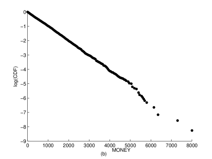
Figure 5: Cumulative distribution function (CDF) of CASE 1 in Table I is drawn for the community of real participants ($3867$ agents).

When $\lambda_{b}$ varies from $1.032$ to $1.08429$ it is observed that the number of non-participants decreases. This is because the chaotic map expands and its resulting projections on axis $x$ and $y$ grow in range, taking a greater group of $i$ and $j$ values is computed. Taking these non-participants off the final money distributions, and so their money too, one can obtain the final CDF’s for the different values of $\lambda_{b}$. When these distributions are depicted an interesting progression is shown. As $\lambda_{b}$ increases, these distributions diverge from the exponential shape.

Fig. 6 shows the representation of simulation cases $1$ to $5$ in a natural log plot up to a range of $\$2000$. It can be appreciated that as $\lambda_{b}$ increases, the straight shape obtained for the symmetric case bends progressively, the probability of finding an agent in the state of poorness increases. It also can be seen that for cases 3 and 4, no agent can be found in a middle range of wealth (from $1000\$$ to $2000\$$). This means that the distribution of money is becoming progressively more unequal.

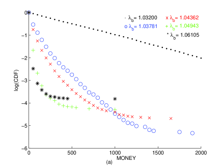
Figure 6: Representations up to $2000\$$ dollars of the final CDF’s obtained for simulation cases 1,2,3,4 and 5 (see Table I).

Figure 7: Representations from $2000\$$ dollars of the final CDF’s obtained for simulation cases 6,7, and 8 (see Table I).

In Fig. 7 the CDF’s for simulation cases $6$ to $8$ are depicted from a range of $2000\$$ and in double decimal logarithm plot. Here, a minority of agents reach very high fortunes, what explains, how other majority of agents becomes to the state of poorness. The data seem to follow a straight line arrangement for case $6$, which resembles a Pareto distribution. Cases $7$ and $8$ show two straight line arrangements which can also be adjusted to two Pareto distributions of different slopes.

Fig. 6 and 7 show how the community is becoming more unequal as $\lambda_{b}$ increases. The rich gets richer as the asymmetry of the chaotic selection of agents increases and the final amount of money of this class is almost the total money in the system. In the other side of the society, the proportion of the population that ends in the state of poverty increases as as $\lambda_{b}$ increases.

What is happening here is, that the asymmetry of the chaotic map is selecting a set of agents preferably as winners for each transaction ($j$ agents). While others, with less chaotic luck become preferably looser ($i$ agents). This is due to the asymmetry of Rule 2, where agent $i$ always decrements his money, and the asymmetry of coordinates $x_{i}$ and $y_{i}$ in the Logistic bimap used for the selection of agents. This double asymmetry makes some agents prone to loose in the majority of the transactions, while a few others always win.

IV Conclusions

This work introduces chaotic dynamics in economic (ideal) gas-like models for trading markets. It shows that introducing chaotic parameters in two different scenarios leads to the referenced money distributions seen in real economies (the Gamma, Exponential and Pareto distributions).

New and interesting results are observed in these scenarios, in the sense that restriction of commercial relations is observed, as well as a different asymptotic wealth distribution depending on the rule of money exchange. It seems that the asymmetry of the trading rule and also of the chaotic selection of agents leads to less equitable distributions of money, meaning that this type of the markets operate under ”unfair“ or asymmetric conditions.

More over, under these assumptions, it illustrates how a small group of people can be chaotically destined to be very rich, while the bulk of the population ends up in state of poverty. This may resemble some realistic conditions, showing how some individuals can accumulate big fortunes in trading markets, as a natural consequence of the intrinsic asymmetric conditions of real economy.

Acknowledgements The authors acknowledge some financial support by Spanish grant DGICYT-FIS200612781-C02-01.

References

- [1] R. Mantegna and H.E. Stanley. An Introduction to Econophysics: Correlations and Complexity in Finance. Cambridge University Press, ISBN 0521620082, 2000.
- [2] V.M. Yakovenko, Econophysics, Statistical Mechanics Approach to, Encyclopedia of Complexity and System Science, ISBN 9780387758886, Springer, 2009. (Available at arXiv:0709.3662v4).
- [3] A.A. Dragulescu and V.M. Yakovenko, Statistical Mechanics of Money, The European Physical Journal B, Vol. 17, pp. 723-729, 2000. (Available at arXiv:cond-mat/0001432).
- [4] A. Chakraborti and B.K. Chakrabarti, Statistical Mechanics of Money: How Saving Propensity affects its Distribution, The European Physical Journal B, Vol. 17, pp. 167-170, 2000.
- [5] J.P. Bouchaud and M. Mézard, Wealth Condensation in a Simple Model Economy, Physica A, Vol. 282, pp. 536-545, 2000.
- [6] B.K. Chakrabarti and S. Marjit, Self-organization in Game of Life and Economics, Indian Journal Physics B, Vol. 69, pp. 681-698, 1995.
- [7] A.A. Dragulescu and V.M. Yakovenko, Exponential and Power-law Probability Distributions of Wealth as Income in the United Kingdom and the United States, Physica A, Vol. 299, pp 213-221, 2001. (Available at arXiv:cond-mat/0103544v2).
- [8] S. Sinha Evidence of the Power-law Tail of the Wealth Distribution in India, Physica A, Vol. 359, pp 555-562, 2006.
- [9] A.Y. Abul-Magd, Wealth Distribution in an ancient Egyptian Society, Phys. Rev. E, Vol. 66, 057104, 2002.
- [10] V. Pareto, Cours d’Economie Politique, F. Rouge, Lausanne and Paris, 1897
- [11] D.G. Champernowne, A Model of Income Distribution, Econ. J., Vol. 63, 318-351, 1953.
- [12] D.G. Champernowne and F.A. Cowell. Economic Inequality and Income Distribution. Cambrige University Press, Cambridge, 1999.
- [13] A. Chatterjee, S. Yarlagadda and B.K. Chakrabarti (eds). Econophysics of Wealth Distributions. Springer Verlag, Milan, 2005.
- [14] B.K. Chakrabarti, A. Chakraborti and A. Chatterjee (eds). Econophysics ans Sociophysics: Trends and Perpectives. Willey-VCH, Berlin, 2006.
- [15] A. Dragulescu and V.M. Yakovenko,Evidence for the Exponential Distribution of Income in the USA, Eur. Phys. J. B, Vol. 20, pp 585-589, 2001.
- [16] J. González-Estévez, M.G. Cosenza, O. Alvarez-Llamoza and R. López-Ruiz, Transition from Pareto to Boltzmann-Gibbs Behavior in a Deterministic Economic Model, Physica A, to appear, 2009.
- [17] M. Patriarca, A. Chakraborti and K. Kaski, Gibbs versus non-Gibbs Distributions in Money Dynamics, Physica A, Vol. 340, pp 334-339, 2004. (Available at arXiv:cond-mat/0312167v1).
- [18] M. Hénon, A Two-dimensional Mapping with a Strange Attractor, Communications in Mathematical Physics, Vol. 50, pp 69-77, 1976.
- [19] R. López-Ruiz and Pérez-Garcia, Dynamics of Maps with a Global Multiplicative Coupling, Chaos, Solitons and Fractals, Vol.1, pp 511-528, 1991.
- [20] R. López-Ruiz, J. Sañudo and X. Calbet, Geometrical Derivation of the Boltzmann Factor, Am. J. Phys., Vol. 76, pp. 780-781, 2008.
- [21] C. Pellicer-Lostao, R. López-Ruiz. Economic Models with Chaotic Money Exchange. Proceedings of the ICCS 2009, Lectures Notes of Computer Sciences, Part I, Vol. 5544, pp. 43-52, 2009. (Available at arXiv:0901.1038).