2-D simulations of FU Orionis disk outbursts

Abstract

We have developed time-dependent models of FU Ori accretion outbursts to explore the physical properties of protostellar disks. Our two-dimensional, axisymmetric models incorporate full vertical structure with a new treatment of the radiative boundary condition for the disk photosphere. We find that FU Ori-type outbursts can be explained by a slow accumulation of matter due to gravitational instability. Eventually this triggers the magnetorotational instability, which leads to rapid accretion. The thermal instability is triggered in the inner disk but this instability is not necessary for the outburst. An accurate disk vertical structure, including convection, is important for understanding the outburst behavior. Large convective eddies develop during the high state in the inner disk. The models are in agreement with Spitzer IRS spectra and also with peak accretion rates and decay timescales of observed outbursts, though some objects show faster rise timescale. We also propose that convection may account for the observed mild-supersonic turbulence and the short-timescale variations of FU Orionis objects.

1 Introduction

The FU Orionis systems are a small but remarkable class of young stellar objects which undergo outbursts in optical light of 5 magnitudes or more (Herbig, 1977). While the rise times for outbursts are usually very short ($\sim 1-10\rm yr$), the decay timescales range from decades to centuries. In outbursts, they exhibit F-G supergiant optical spectra and K-M supergiant near-infrared spectra dominated by deep CO overtone absorption. The FU Ori objects also show distinctive reflection nebulae, large infrared excesses of radiation, wavelength dependent spectral types, and “double-peaked” absorption line profiles (Hartmann & Kenyon, 1996). The accretion disk model for FU Ori objects proposed by Hartmann $\&$ Kenyon (1985, 1987a, 1987b) and Kenyon et al. (1988) can explain the peculiarities enumerated above in a straightforward manner.

Bell $\&$ Lin (1994) suggested that the thermal instability (TI) was responsible for FU Ori outbursts. To agree with the outburst mass accretion rates ($\sim 10^{-4}\rm M_{\odot}\,yr^{-1}$) and the outburst duration time ($\sim 100$ yr), with the TI, Bell $\&$ Lin used very low viscosities both before and after the outbursts. However, this theory predicts that the outburst is confined to inner disk radii $\lesssim 0.1\rm AU$, whereas Zhu et al. (2007, 2008) found that the high accretion rate region must extend to $\gtrsim 0.5\rm AU$, based on modeling Spitzer IRS data.

Bonnell & Bastien (1992) suggested that a binary companion on an eccentric orbit could perturb the disk and cause repeated outbursts of accretion. However, in the case of FU Ori, no close companion is known, and no radial velocity variation has been detected (Petrov & Herbig, 2008). Vorobyov $\&$ Basu (2005, 2006) suggested that gravitational instabilities might produce the non-steady accretion, but could not carry out the calculation within the inner disk; thus the details of the accretion event are uncertain. Lodato & Clarke (2004) suggested that planets might dam up disk material until a certain point, resulting in outbursts. This model also depends upon the TI and assumes a very low viscosity as in Bell $\&$ Lin (1994).

The rediscovery and application of the magnetorotational instability (MRI) to disk angular momentum transport have revolutionized our understanding of accretion in ionized disks (e.g. Balbus $\&$ Hawley 1998 and references therein). However, it was recognized that T Tauri disks are cold and thus likely to have such low ionization levels that the MRI cannot operate, at least in some regions of the disk (e.g., Reyes-Ruiz $\&$ Stepinski 1995). Gammie (1996) suggested that nonthermal ionization by cosmic rays could lead to accretion in upper disk layers, with a ”dead zone” in the midplane. This picture implies that accretion is not steady throughout the disk, and the mass should pile up at small radii.

Armitage et al. (2001) considered the time evolution of layered disks including angular momentum transport by the gravitational instability (GI). Within a certain range of mass addition by infall in the outer disk, they obtained episodic outbursts of accretion at $\sim 10^{-5}\rm M_{\odot}\,yr^{-1}$ lasting $\sim 10^{4}$ yr. However, these outbursts are too weak and last too long compared with FU Ori outbursts. Gammie (1999) and Book & Hartmann (2004) were able to get outbursts more like FU Ori behavior with a different set of parameters. The Armitage, Gammie, Book & Hartmann models were vertically averaged and had schematic treatments of radial energy transport.

Earlier models of layered disk evolution have been based on phenomenological one-zone, or two-zone, models for the vertical structure of the disk. It is quite difficult to formulate these models in a consistent way, particularly near transition radii where the temperature or ionization structure of the disk changes sharply and radial energy transport may be important. To make progress it is necessary to consider more accurate vertical structure and more accurate energy transport models.

In this paper, we construct two-dimensional (axisymmetric) layered disk models. We find that the MRI triggering by the GI can explain FU Ori-type outbursts if the MRI is thermally activated at T_M$\sim$1200 K. In §2, the equations and methods of the 2D models are introduced. In §3, outburst behavior is described. In §4, we focus on vertical structure and convection in the disk. We discuss implications of the 2D simulations compared with observations in §5, and summarize our results in §6.

2 Methods

In this work we are particularly interested in accurately modeling the flow of energy within the disk. A full treatment would numerically follow the development of MRI, GI, and radiative, convective, and chemical energy transport in 3D. As this is not yet possible, we use the phenomenological $\alpha$-based viscosity to represent the angular momentum transport by the MRI and GI and heating by dissipation of turbulence. An accurate treatment of energy balance (viscous heating and radiative cooling) is essential to understand the outburst, especially for the thermal instability. We implemented the realistic radiative cooling in the ZEUS-type code of McKinney& Gammie (2002).

To test our code, we set a hot region in an optically thick disk region and then let the radiative energy diffuse without evolving the hydrodynamics. The hot region expands nicely in a round shape in R-Z space with the correct flux. We have also tested the total energy conservation during our outburst simulations, finding that the energy deficit during outburst is only $<$ 1% of the total energy radiated.

2.1 Viscous heating

The momentum equation and energy equations are

$$\rho\frac{Dv}{Dt}=-\nabla p-\rho\nabla\Psi-\nabla\cdot\Pi\,,$$ (1)

$$\rho\frac{D}{Dt}\left(\frac{e}{\rho}\right)=-p\nabla\cdot v+\Phi-\Lambda\,.$$ (2)

Here, as usual, $D/Dt\equiv\partial/\partial t+v\cdot\nabla$ is the Lagrangian time derivative, $\rho$ is the mass density , $v$ is the velocity, $e$ is the internal energy density of the gas, $p$ is the gas pressure, $\Psi$ is the gravitational potential, and $\Lambda$ is the radiative cooling rate. The dissipation function $\Phi$ is given by the product of the anomalous stress tensor $\Pi$ with the rate-of-strain tensor $\xi$,

$$\Phi=\Pi_{ij}\xi^{ij}$$ (3)

(sum over indices), where the anomalous stress tensor is the term-by-term product

$$\Pi_{ij}=2\rho\nu_{V}\xi_{ij}S_{ij}$$ (4)

(no sum over indices), where $S_{ij}$ is a symmetric matrix filled with 0 or 1 that serves as a switch for each component of the anomalous stress. In current simulations, we switched on all the component of the anomalous stress. It is not yet known whether any prescription for $\Pi_{ij}$ is a good approximation for modeling MHD turbulence. We set the viscosity coefficient to $\nu_{V}=\alpha(c_{s}^{2}/\Omega)sin^{3/2}\theta$, which vanishes rapidly near the poles (McKinney& Gammie, 2002). $\alpha$ is the viscosity parameter and $\Omega$ is the angular velocity at radius $R$.

The equation of state is

$$p=\left(\gamma-1\right)e\,.$$ (5)

and the sound speed is

$$c_{s}^{2}=\gamma\frac{k_{B}T}{\mu}$$ (6)

where $\gamma$ and $\mu$ are the adiabatic index and the mean molecular weight. We assume $\gamma=5/3$ and $\mu=2.4M_{P}$ where $M_{P}$ is the mass of one proton. The adiabatic index and mean molecular weight will change at different temperatures and pressure (especially during outburst when the disk is fully ionized) and a fully self-consistent treatment would use a tabulated equation of state. We will discuss a more realistic equation of state in a later paper.

2.2 Radiative cooling

In an accretion disk, radiation is the main cooling mechanism, and radiation energy and pressure can affect the disk dynamics. Numerically, there are two different approaches to treat the radiative transport in an accretion disk. One is to solve the full radiative transfer equation

$$\rho\frac{D}{Dt}\left(\frac{E}{\rho}\right)=-\nabla\cdot F-\nabla v:P+4\pi\kappa_{P}B-c\kappa_{E}E$$ (7)

with the material energy equation:

$$\rho\frac{D}{Dt}\left(\frac{e}{\rho}\right)=-p\nabla\cdot v-4\pi\kappa_{P}B+c\kappa_{E}E$$ (8)

in both the optically thick and thin regions by an implicit method (Turner & Stone, 2001; Wünsch et al., 2005; Hirose et al., 2006). Here, as above, $\rho$,$e$,$v$, and $p$ are the gas mass density, energy density, velocity and scalar isotropic pressure respectively, while E,F, and P are the total radiation energy density, momentum density and pressure tensor, respectively. $\kappa_{P}$ and $\kappa_{E}$ are Planck mean and energy mean absorption coefficients. An implicit method is required because of the extremely short time step needed by the explicit method (grid size over the speed of light), but the implicit method is time consuming, requiring solution of an N${}^{2}\times$N² matrix equation at each timestep.

A second, less accurate but less costly, approach is to add a radiative source (heating/cooling) term in the energy equation, use the diffusion approximation in the optically thick region, and use an approximation to treat the optically thin region (Boss, 2002; Boley et al., 2006; Cai et al., 2008). When the radiation pressure is negligible, as in the case for protostellar disks, and the radiation field is nearly in equilibrium ($D(E/\rho)/Dt=0$), equations 7 and 8 become

$$\rho\frac{D}{Dt}\left(\frac{e}{\rho}\right)=-p\nabla\cdot v-\Lambda$$ (9)

where $\Lambda=\nabla\cdot F$ and $F$ is the radiative flux.

We examine the justification for ignoring the advection term (within the term on the left side of Eq. 7) and the term describing work done by radiation on the gas (second term of the right side of Eq. 7) following the criterion given by Mihalas & Weibel Mihalas (1984). If in one system, $L$ is the characteristic size, u is the characteristic velocity and $\tau$ is the optical depth of $L$, the terms describing the advection and the work done by the radiation can be ignored if $\tau\gg$1 and $\tau\times u/c\ll$1, which is called static diffusion limit. This criterion can be simply understood as follows:

The timescale for radiation to propagate across a region of length $L$ and mean optical depth $\tau$ is of order

$$t_{E}\sim L\tau/c\,.$$ (10)

For comparison, the material crossing time of this region is

$$t_{u}\sim L/u\,,$$ (11)

so that the ratio of these two timescales is

$${t_{E}\over t_{u}}\sim{u\over c}\tau\,.$$ (12)

If this ratio is far less than one, the region is in radiative quasi-equilibrium before the material carrying radiation energy away so that the energy emitted and absorbed equals to the diffusion term (Eq. 7). In a 3-D accretion disk, this typical velocity is the Keplerian velocity. However in our 2-D axisymmetric simulation, this velocity is just the mean radial velocity of the gas. Thus, $t_{u}$ is close to the viscous time which is longer than the time for sound to cross a scale height $H$ by a factor of order $\alpha^{-1}(R/H)^{2}$.

In our simulations, even at the maximum temperatures achieved in the innermost disk, $u/c\lesssim 10^{-5}$ (§4) and so the approximation of radiative equilibrium should be valid except at very large optical depths. It turns out that, during the outburst, vertical Rosseland mean optical depths $\sim 10^{4}$ in the innermost disk. Thus our approximation is justified, though it may break down at smaller radii than we have considered here.

In detail, the radiative transfer in the optically thick disk, defined as the region where $\tau>\tau_{thick}$, is given in the diffusion approximation by

$$\Lambda=\triangledown\cdot F,$$ (13)

where the flux $F$ is

$$F=-\frac{16\sigma\beta T^{3}}{\chi_{R}\rho}\triangledown T,$$ (14)

and $\beta$ is the flux limiter,

$$\beta=\frac{2+y}{6+3y+y^{2}}\,,$$ (15)

with

$$y=\frac{4}{\chi_{R}\rho T}\mid\triangledown T\mid\,.$$ (16)

where $\chi_{R}$ is the Rosseland mean of the absorption coefficient.

The optically thin region is more complicated. In this region we restrict our considerations to radiative transport in the vertical direction only. We have developed two methods to solve this problem in collaboration with members of the Indiana disk group (D. Durisen, K. Cai, & A. Boley, 2008, personal communication). The first method considers the cooling rate of every cell in the optically thin region can be written as:

$$\Lambda=\rho\kappa_{P}(T)\left(4\sigma T^{4}-4\pi J(Z)\right)-\rho\kappa_{P}(T_{e})\sigma T_{e}^{4}e^{-\tau_{e}(Z)}\,$$ (17)

where $\kappa_{P}(T)$ is the Planck mean opacity at the temperature $T$, $T_{e}$ is the temperature of the envelope, and also J(Z) and $\tau_{e}(Z)$ are the mean intensity and the optical depth of the envelop at height Z in the disk atmosphere. The first term is the energy emitted by the cell, while the second and third terms are the energy absorbed from the optically thick region and from the envelope. Using the two stream approximation,

$$J(Z)=\frac{1}{4\pi}\int Id\Omega=\frac{1}{4\pi}\left(2\pi I_{+}+2\pi I_{-}\right).$$ (18)

This treatment assumes flux conservation and thus ignores energy dissipation in the atmosphere. The net flux $F_{b}$ from the disk photosphere is then

$$F_{b}=\int I\,\mu\,d\Omega=\pi\left(I_{+}-I_{-}\right)\,,$$ (19)

where $\mu$ is the cosine of the angle measured from the vertical. Thus

$$J(Z)=\frac{1}{2}\left(I_{+}+I_{-}\right)=\frac{F_{b}}{2\pi}+I_{-}(Z).$$ (20)

$F_{b}$ is approximately

$$F_{b}=\frac{4\sigma\left(T_{b}^{4}-T_{e}^{4}\right)}{3\left(\tau_{b}+2/3\right)}$$ (21)

where $T_{e}$ is a term which accounts for the external irradiation (see equation (10) in Boley et al. (2006)). $T_{b}$ and $\tau_{b}$ are the temperature and optical depth of the first optically thick cell right below the photosphere (again, see Boley et al. (2006)).Finally, we must set $I_{-}(Z)$ to obtain a closed expression for $\Lambda$:

$$I_{-}(Z)=\int_{Z}^{\infty}\rho\kappa_{P}\frac{\sigma T(z)^{4}}{\pi}dz+\frac{\sigma T^{4}_{env}e^{-\tau_{en}(Z)}}{\pi}\,.$$ (22)

which is the intensity from the optically thin region above height $Z$. Theoretically, the first term should also have e^-τ. However, since we only consider the optically thin region here, we ignore it to simplify the calculation and save computational time.

The second method is much simpler but limited to this particular problem with no irradiation. As we do not consider irradiation, we can use the usual gray atmosphere result. Without the third term in equation (17), we have

$$\Lambda=\rho\kappa_{P}(T)\left(4\sigma T^{4}-4\pi J(Z)\right)\,,$$ (23)

and in a gray case

$$J=\frac{\sigma}{\pi}T^{4}(Z)=\frac{\sigma}{\pi}\left(\frac{3}{4}T_{eff}^{4}(\tau+\frac{2}{3})\right)\,,$$ (24)

where $T_{eff}$ is given by the boundary flux $F_{b}=\sigma T_{eff}^{4}$ as equation 21. In detail, counting $\theta$ grid cell index i as increasing with increasing $\theta$ and $\tau$, we set the first grid with $\tau(R,\theta_{i})>3$ as the boundary grid and $\tau_{b}$=$\tau(R,\theta_{i})$. Then we derive the effective temperature (or equivalently, the boundary flux) using the gray approximation

$$F_{b}=\sigma T_{eff}^{4}=\frac{4\sigma T_{b}^{4}}{3(\tau_{b}+2/3)}\,.$$ (25)

With $T_{eff}$, we use equation 24 to set the temperatures of all cells at $R$, $\theta<\theta_{i}$, and use the diffusion equation (14) at all $r,\theta\geq\theta_{i}$. This way of matching the ”optically thin” (gray) atmosphere to the ”optically thick” (diffusion equation) interior removes the temperature jump seen at the boundary between the two treatments seen in the simulations of Cai et al. (2008).

Both methods give similar results if there is no irradiation(see Appendix A) - basically, they are the same except for the assumed directionality of the radiation field. We use the second method in this paper, although the first method is of interest for cases in which external irradiation is important.

We have adopted the Bell & Lin (1994) opacity fits to facilitate comparison with previous calculations (Bell & Lin, 1994; Armitage et al., 2001); subsequent improvements in low-temperature molecular opacities will modify results at low temperatures (Zhu et al 2009), but should not substantially affect the outburst behavior driven at higher temperatures.

2.3 Angular Momentum Transport

To complete the model we need a prescription for the dimensionless viscosity $\alpha$. The key physics we want to capture is the dependence of the MRI and GI transport on position in the disk (see, e.g., Miller & Stone 2000 for MRI activity as a function of height in the disk).

For the MRI, we set $\alpha_{M}=0.1$ when $T>T_{M}$, where $T_{M}$ is a critical temperature (typically $1200\rm K$) where thermal ionization makes the disk conductive enough to sustain the MRI. In addition we calculate $\Sigma_{+}=\int_{0}^{\theta}Rd\theta^{\prime}\rho$ (and in models where the disk is not assumed to be symmetric about the midplane, $\Sigma_{-}=\int_{\theta}^{\pi}Rd\theta^{\prime}\rho$) and set $\alpha_{M}=0.1$ if $\Sigma_{+}$ or $\Sigma_{-}<\Sigma_{crit}$, where $\Sigma_{crit}$ is the maximum surface density of the MRI active layer on one side of the disk (In our current model we assume $\Sigma_{crit}$=50 g cm^-2 ). Otherwise the disk is magnetically ’dead’ and $\alpha_{M}=0$. Also to avoid the strong MRI viscous heating at the disk’s upper photosphere with very low density, we set $\alpha=0$ for the region with $\tau<10^{-3}$.

The value of $\alpha_{M}$ predicted by theory is uncertain, with widely-varying estimates depending upon mean magnetic fluxes, magnetic Prandtl numbers, and other assumptions (Guan et al. 2008, Johansen & Levin 2008, Fromang et al. 2007). Given these uncertainties, observational constraints take on special significance. A recent review of the observational evidence by King, Pringle, & Livio (2007) argues that $\alpha_{M}$ must be large, of the order 0.1-0.4, based in part on observations of dwarf novae and X-ray binaries where there is no question of gravitational instability. Our empirical study of FU Ori, where we were able to constrain the radial extent of the high accretion state, implies values of $\alpha\sim 0.1$. (Zhu et al. 2007).

For the GI, we calculate the Toomre $Q$ parameter

$$Q={c_{s}\Omega\over\pi G\Sigma}\,.$$ (26)

When $Q\sim 1$ the disk is gravitationally unstable. Full global models (Boley et al., 2006) and physical arguments (Gammie 2001) suggest that if the disk is sufficiently thin angular momentum transport by GI is localized and can be crudely described by an equivalent $\alpha$. We set

$$\alpha_{Q}(R,\theta)=e^{-Q(R)^{2}},$$ (27)

which is independent of $\theta$. This has the sensible effect of turning on GI driven angular momentum transport when $Q<2$ and turning off GI driven angular momentum transport when $Q$ is large. In regions with both GI and MRI we set $\alpha=\alpha_{M}$ (in these regions $\alpha_{M}\gg\alpha_{Q}$).

The maximum $\alpha_{Q}$ is $<$0.1 during the simulations, consistent with our assumption that fragmentation does not occur. Our prescription for $\alpha_{Q}$ on Q is heuristic and other forms are plausible. Gammie (2001) and Lodato & Rice (2004, 2005) found that the amplitude of GI depends on the cooling rate in addition to Q; and Balbus & Papaloizou (1999) argued that the angular momentum flux carried by GI is a global effect and the local viscosity description can only be valid near the corotation radius. However, using self-consistent cooling, Boley et al. 2006 showed that the $\alpha_{GI}$ agrees with the Gammie description very well, which assumes that the GI viscous heating is locally balanced by the cooling. Recent smooth particle hydrodynamics SPH simulations by Cossins et al. (2009) also showed that GI disks with tightly wound spiral arms can be approximated by a local treatment.

3 2D results

We use spherical polar coordinates and assume axisymmetry in all our simulations. To sample both the inner disk and the outer disk, we use a logarithmic radial grid (radial grids are uniform in log(R-R_in)) from 0.06-40 AU and a uniform $\theta$ grid in $(0.5\pm 0.15)\pi$. This gives adequate radial resolution for both the inner and outer disk, and spans a large enough range in $\theta$ to include the optically thick region of the disk. Parameters for all the 2D simulations are listed in Table 1.

3.1 Initial and Boundary Conditions

All our disk models begin with the initial temperature distribution

$$T(R,\theta)=300(R/AU)^{-1/2}\rm K,$$ (28)

and $\rho=\Sigma(R)/(H{2\pi}^{1/2})\exp(-R^{2}\theta^{2}/(2H^{2}))$, $H\equiv c_{s}/\Omega$ from 0.4-100 AU , so the disk is approximately in dynamical equilibrium. We set $\Sigma(R)$ using a $\dot{M}$=10^-5 M_⊙/yr constant $\alpha$ ($\alpha=0.1$) one-zone accretion disk model (see Equation 3 in Whitney et al. (2003)). Although this is not an exact steady-state model, the disk relaxes rapidly at the beginning of the simulation.

We apply outflow boundary conditions (Stone & Norman, 1992) to all boundaries. In some simulations the disk is assumed to be symmetric about the midplane to reduce computational cost; for these half-disk simulations we use a reflecting boundary condition (Stone & Norman, 1992) at the midplane. The inner boundary is set to either 0.06 AU, 0.1 AU, or 0.3 AU to examine how different inner radii affect disk evolution. These parameters are listed in Table 1.

We follow the evolution of the disk for 10⁵ years. Typically several outbursts occur during the simulation. After the first outburst, the subsequent outbursts are similar and do not depend on the initial condition. Thus, we use the disk density and temperature distribution after the first two outbursts as the new initial condition to study the third outburst for various 1D and 2D models. The disk mass for this initial condition is $\sim$ 0.5 $\rm M_{\odot}$.

3.2 Outbursts

In the protostellar phase, the disk is unlikely to transport mass steadily from $\sim$100 AU all the way to the star at an accretion rate matching the mass infall rate $10^{-6}-10^{-4}\rm M_{\odot}\,yr^{-1}$ from the envelope to the outer disk. The outburst sequence we find here is qualitatively similar to that found by Armitage et al. (2001), Gammie (1999), and Book & Hartmann (2001). Mass added to the outer disk moves inwards due to GI, but piles up in the inner disk as GI becomes less effective at small R. Eventually, the large $\Sigma$ and energy dissipation leads to enough thermal ionization to trigger the MRI. Then the inner disk accretes at a much higher mass accretion rate, which resembles FU Orionis-type outbursts. After the inner disk has drained out and becomes too cold to sustain the MRI, the disk returns to the low state. During the low state mass continuously accretes from large radius (or from an infalling envelope) causing matter to pile up at the radius where GI becomes ineffective yet again, leading to another outburst.

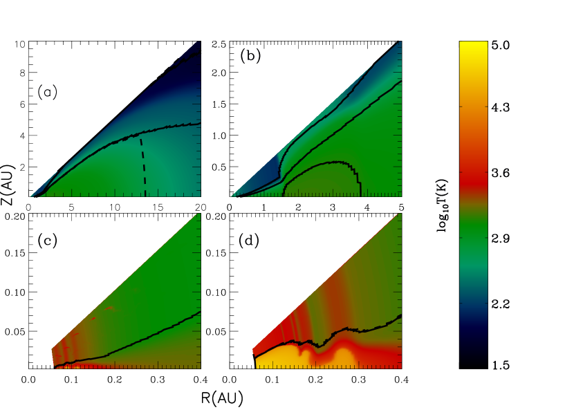
Figure 1: The disk’s temperature color contours at four stages during the outburst in R-Z coordinate. The black curves are the $\alpha$ contours which also outlines different regions in the disk. The vertical dashed line in Panel (a) shows $\alpha_{Q}=0.025$. (a) is the stage before the outburst. (b) represents the stage when the MRI is triggered at 2 AU. (c) represents the moment when the TI is triggered at the innermost region. (d) is the stage when the TI is fully active within 0.3 AU.

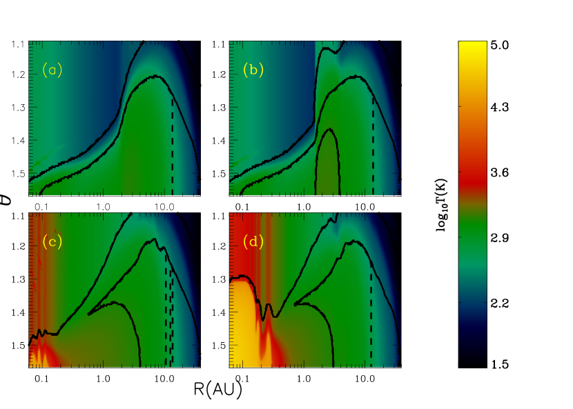
Figure 2: The disk’s temperature color contours at four stages during the outburst, the same as Fig. 1. The black curves are the $\alpha$ contours which also outlines different regions in the disk: the uppermost atmosphere, active layer, and the dead zone close to the midplane. The dashed line shows $\alpha_{Q}=0.025$. (a) is the stage before the outburst. (b) represents the stage when the MRI is triggered at 2 AU. (c) represents the moment when the TI is triggered at the innermost region. (d) is the stage when the TI is fully active within 0.3 AU.

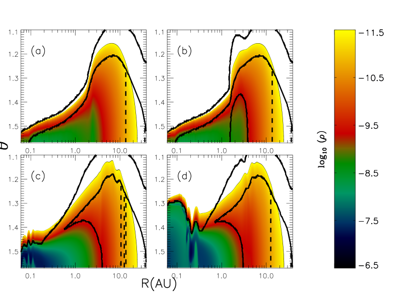
Figure 3: Similar to Figure 2 but shows the density contours. The high density white regions close to the midplane in (c) and (d) correspond to the region at the TI low state in Figure 2. Because it is much colder than the midplane which is at the TI high state, it needs a high density to balance the pressure.

Figures 1- 5 show the disk temperature and density structure at four consecutive stages of the outburst for our fiducial model. Figure 1 is shown in R-Z coordinate while figures 2 and 3 are shown in log₁₀R-$\theta$ coordinates (R from 0.06 to 40 AU, $\theta$ from 1.1 to $\pi/2$). Since the GI, MRI and TI are taking place at quite different radii, most of our plots are in log₁₀R-$\theta$ coordinates so that all of them can be seen in one figure, although it is less intuitive than R-Z coordinates. The black solid curves plotted on top of the color contours delimit regions of differing $\alpha$. Regions above the top solid curve limit the low-$\rho$ photosphere with $\tau<10^{-3}$ to $\alpha=0$. Between the top and next lower solid curve lies the MRI-active layer with $\Sigma_{+}$¡50 gcm^-1 and $\alpha=\alpha_{M}=0.1$. Regions below the two solid curves constitute the ”dead zone” with only $\alpha_{Q}$ if any. The vertical dashed lines at large radii represent $\alpha_{Q}=0.025$.

Panel (a) of Figures 1-3 show the disk temperature structure before the outburst. The disk is too cool to sustain any MRI except in the active layer. The contours in Figures 1-3 show the outer disk (R¿1AU) is geometrically thick, with a ratio of vertical scale height H to radius H/R$\sim$0.2, and massive, while the inner disk is thin with a low surface density. The inner disk is stable against GI and cannot transport mass effectively. The mass coming from the GI driven outer disk piles up at several AU. The GI thus gradually becomes stronger at several AU and the disk heats up.

The disk midplane temperature at 2 AU eventually reaches the MRI trigger temperature (T${}_{M}\sim$1200 K) and MRI driven angular momentum transport turns on. Panel (b) of Figures 1-3 show the stage when the thermal-MRI is triggered at the midplane around 2AU. The thermal-MRI active region are outlined by the semicircular $\alpha$ contour around 2 AU in these figures. After the MRI is activated, $\alpha$ increases from $\alpha_{Q}(2AU)\sim 0.01$ to $\alpha_{M}=0.1$, which leads to a higher mass accretion rate. Afterwards, the MRI active region expands both vertically and radially until the whole inner disk becomes fully MRI active.

As more and more mass is transferred to the inner disk, the temperature continues to rise. At $T\sim 4000\rm K$ the disk becomes thermally unstable and $T$ rises rapidly to $\sim 2\times 10^{4}\rm K$. Panel (c) of Figures 1-3 show the moment the TI is initiated in the innermost disk. With the temperature leap, the pressure of the TI active region also increases significantly. Thus the TI active region expands and compresses the TI non-active region, leading to a lower density of the TI active region than nonactive region (lower density at midplane around 0.1 AU in panel (c) of Fig. 3).

Panel (d) of Figures 1-3 show that after the TI is triggered in the innermost disk, the TI front travels outwards to $\sim$ 0.3 AU until the entire inner disk is in a ”high state.” The hot inner disk (R¡0.2 AU) is puffed up to H/R$\sim$0.15. The mass accretion rate is $2\times 10^{-4}\rm M_{\odot}\,yr^{-1}$ at this stage. The central temperature has a sharp drop at 0.3 AU, beyond which the disk is in a thermally stable state at $T\simeq 3000\rm K$. Details of the TI are discussed in Appendix B. At this transition from the high to low state around $0.2\rm AU$, some temperature and density fluctuations are present, which results from convection. We will discuss convection in detail in §5.

The TI high state (T_c¿10,000 K, panel (d) of Fig. 1-3) lasts for $\sim$10² years, draining the inner disk (R ¡ 0.5 AU) until it is not massive and hot enough to sustain the TI high state; it then returns to the TI low state. The inner disk may temporarily return to the high state due to MRI-driven mass inflow but eventually mass is drained from the MRI active region, it becomes MRI inactive, and the disk returns to the state shown in panel (a).

Figure 4 shows the vertically integrated surface density at the above stages. Before the outburst, the surface density peaks around 2 AU (long-dash curve); this radius divides the inner, GI stable disk from the outer GI unstable disk. Once the MRI is triggered at 2 AU, it transports mass into the inner disk effectively. At the moment the TI is triggered (dotted curve), the surface density of the inner disk is already one order of magnitude higher than that before the MRI is triggered. During the TI fully active stage (solid curve), the relatively low surface density region within 0.3 AU corresponds to the TI high stage with T_c¿10⁴ K. The density fluctuations around 0.3 AU result from convection at the transition between the TI high and low states as seen in Figures 1 and 3. We discuss the details of convection in §4.3

Figure 5 shows the effective temperature distributions at the same stages as above. When the MRI is triggered, the effective temperature increases dramatically with the increasing accretion rate. Eventually the whole inner disk almost accretes at a constant rate and the effective temperature is similar to that of a steady accretion solution at $M\dot{M}=1.8\times 10^{-4}M_{\odot}^{2}yr^{-1}$ (smooth solid curve). The discrepancy at small radii may be caused by the outflow inner boundary condition of the 2D simulation, which means all the velocity gradients relative to the coordinates (R, $\theta$) are 0.

3.3 Resolution Study

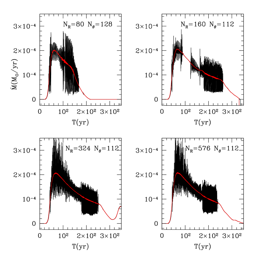
Figure 6: The disk’s mass accretion rate through the innermost boundary with time for models with four different resolutions. The red lines are the mass accretion rates after being smoothed.

Figure 6 shows the mass accretion rates during an outburst for models with four different numerical resolutions. In general the vertical linear resolution must be higher than the radial linear resolution to resolve the vertical structure of the disk, particularly the exponential density drop in the disk photosphere. With $N_{R}=320$ grid cells and $N_{\theta}=112$ grid cells, every grid is 5 times longer radially than vertically.

The simulations have a similar maximum mass accretion rate and outburst timescale as long as $N_{R}\gtrsim 100$ grid cells. This suggests that the models are, crudely speaking, converged.

Notice that models with N${}_{R}\geq 324$ grid cells have complex substructure during outburst. This is caused by convection in the TI high state region. Lower resolution models barely resolve the convective eddies and thus damp away this substructure.

3.4 Boundary effects

We have also explored the effect of varying the inner boundary radius $R_{in}$ on the models. Figure 7 shows $\dot{M}(t)$ for a set of models with $0.06\rm AU\leq R_{in}\leq 0.3\rm AU$, with one two-sided (not equatorially symmetric) model at $R_{in}=0.06\rm AU$. All models have $N_{R}=320$ and $N_{\theta}=112$, except the two-sided model, which has $N_{\theta}=224$.

The outburst amplitude and duration are nearly independent of $R_{in}$ as long as $R_{in}$ is far enough in that the TI can be triggered; the TI is not triggered when $R_{in}=0.3\rm AU$, and so the outburst is slightly stronger and shorter. One implication of the lack of sensitivity of the outburst profile to $R_{in}$ is that, while the TI can sharpen the outburst slightly, the outburst timescale and maximum mass are largely set in the outer disk: where the MRI becomes active, how much mass is accumulated during the quiescent stage, and so on.

When the TI is triggered, $\dot{M}(t)$ exhibits strong short-timescale variations (panel (b,c,d) of Fig. 7). This is caused by convection during the transition between the TI high and low states; the large temperature gradients at the transition make it highly convectively unstable by the Schwarzschild criterion (see §4 for details).

Convection at the high state-low state transition radius changes the character of the $\dot{M}(t)$ variability in 2D models compared to 1D (vertically averaged) models. In 1D evolution models flickering at any radius will propagate through the entire inner disk, making the entire inner disk flicker between the low and high states. Thus the mass accretion rate varies violently during 1D evolutions. To avoid this, Bell & Lin (1994) used an $\alpha$ prescription designed to make $\alpha$ increase sharply from the low to the high states. In 2D models, on the other hand, flickering propagates both radially and vertically. For example, consider a region near the midplane that wants to jump to the high state will soon experience convective cooling and return to the low state. This acts to localize and dampen low state-high state flickering.

For models with $R_{in}=0.06\rm AU$ (panel (c) in Fig. 7), $\dot{M}(t)$ varies less violently than in models with $R_{in}=0.1\rm AU$ because the inner edge is far from the convection associated with the low state high state transition. As the resolution increases, however, the $R_{in}=0.06\rm AU$ model becomes more and more variable. These models, and especially the convection zones, are not converged even at our highest resolution. This is not a major concern, as the fine structure of convection in our axisymmetric, phenomenological $\alpha$ viscosity model will not be the same as the fine structure of convection in a three dimensional, MHD turbulent disk; further resolving this structure would not improve the model.

One aspect of the details of convection is worth commenting on. Panel (d) in Figure 7 shows a full-disk model, which exhibit less variability than the half-disk models. Convection in the full-disk models can penetrate, rather than reflecting back from, the midplane. This feature of disk convection is consistent with linear theory (Ruden et al. 1988), which shows that the most unstable mode has no nodes in $v_{z}$. Because the maximum mass accretion rates and the outburst duration times are similar for half-disk and full-disk models, most of our simulations have been carried with one-sided models to save computation time. However, we need to use the full-disk models to study convection during the outburst.

4 Vertical Structure and Convection

Though our 2D simulations exhibit complex time-dependent behavior, the vertical structure of the simulated disk can be well fit by a simple analytical calculation plus some basic assumptions.

Assuming local energy dissipation and with a given effective temperature and viscosity parameter $\alpha$, the disk structure can be defined by the following equations. Assuming all the viscosity-generated energy radiates vertically, we have

$$\frac{9}{4}\nu_{V}\rho\Omega^{2}=\frac{d}{dz}\left(F\right)\,,$$ (29)

where the vertical flux $F$ is

$$F=\frac{4\sigma}{3}\frac{dT_{\tau}^{4}}{d{\tau}}\,,$$ (30)

the viscosity is

$$\nu_{V}=\alpha c_{s}^{2}/\Omega\,,$$ (31)

and

$$d\tau=-\rho\kappa(T,p)dz\,\,.$$ (32)

With hydrostatic equilibrium,

$$\frac{dp}{dz}=-\frac{GM_{*}\rho z}{R^{3}}\,,$$ (33)

and the equation of state,

$$p=\frac{k_{B}}{\mu}\rho T\,.$$ (34)

$\rho$,$T$, and $p$ are functions of Z. Equation 29 can be integrated towards the midplane given $T_{eff}=T(\tau=2/3)$ as the boundary condition. The integration is halted at $z_{f}$, where the total viscous heating is equal to $\sigma T_{eff}^{4}$. In general $z_{f}\neq 0$ so we change the initial conditions and repeat the integration until $z_{f}=0$, in which case we have the self-consistent vertical structure solution. This procedure is identical to that described in Zhu et al. (2009); we will call these local vertical multi-zone (LVMZ) models.

Figure 9 shows the vertical structure at 0.1 AU from the 2D simulation and that from the LVMZ with the same central temperature. Though the 2D model cannot resolve the region where $T\sim$ $10^{4}K$, the 2D model otherwise agrees with the LVMZ very well, which means that at 0.1 AU the local treatment is a good approximation even during the TI high state, and that radial energy transport is not important. We find that in general the simulation follows the ’S’ curve calculated by the LVMZ very well during the whole TI activation process (see Appendix B).

In the lower left panel of Figure 9, the pressure plateau around $\tau\sim 10$ is caused by the rapid increase in opacity with increasing temperature near $\sim 10^{4}K$ as H ionizes (see the appendix in Zhu et al. 2009). This means that the optical depth can change significantly while the pressure remains nearly the same.

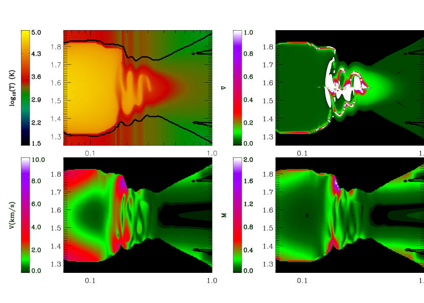
Figure 10: The contours for the temperature, temperature gradient, velocity and Mach number at the TI active stage. The white regions in the temperature gradient contour are due to the gradient larger than the shown range from 0 to 1. The optically thin region has been masked off in order to have the convective patterns in the optically thick region stand out.

The large vertical temperature gradient causes this region to become convectively unstable. As shown in the lower right panel, the dense gas is on top of the thin gas at $\tau<100$ which is clearly unstable against convection or Rayleigh-Taylor instability. Though this convective region is only at the surface and barely resolved at 0.1 AU, it extends to the whole disk at 0.2 AU, where convective patterns even penetrate the mid-plane (Fig. 10).

Convection occurs wherever the Schwarzschild criterion is violated: $\nabla_{S}\equiv d\log T/d\log P>(\gamma-1)/\gamma=0.4$ in our case ($\gamma=5/3$). For an optically thick disk, if the opacity can be described as $\kappa=\kappa_{0}T^{\beta}P^{\epsilon}$ (Bell & Lin, 1994; Zhu et al., 2009), Rafikov (2007) derives $\nabla_{S}>$(1+$\epsilon$)/(4-$\beta$). Thus, the disk is convectively unstable when its temperature is in the range with the opacity satisfying (1+$\epsilon$)/(4-$\beta$)¿($\gamma-1$)/$\gamma$=0.4 .

Before the outburst, the disk is convectively stable. The active layer has a lower temperature than the dust sublimation temperature. Thus, $(1+\epsilon)/(4-\beta)\simeq 0.3$, using the Bell & Lin (1994) opacities. The numerical simulation also shows $\nabla_{S}$ is slightly smaller than ($\gamma-1$)/$\gamma$=0.4, which implies it is convectively stable. The dead zone is isothermal without any energy generation, which means it is also convectively stable with $\nabla_{S}\sim$0.

During the TI high state, however, the disk exhibits a variety of convective features at $R<0.6\rm AU$, where $T>2000\rm K$. The inner disk consists of three distinct convective regions:

1) At $0.35\rm AU<R<0.6\rm AU$, the disk is hot enough that the dust has sublimated and the gas is in molecular form ($2000\rm K<T<5000\rm K$) with TiO and H₂O opacities dominating the opacity. Based on the opacity given by Bell & Lin (1994), $(1+\epsilon)/(4-\beta)\sim$1 so that the disk is convectively unstable. Our numerical simulations have also shown that $\nabla_{S}>0.4$ in these regions (changing from 0.4 at $R\sim 0.6\rm AU$ to 1 at $R\sim 1\rm AU$). However, convection turns out to be inefficient in these regions, with convective speeds far less than the sound speeds (lower right panel of Fig. 10).

2) At 0.15 AU ¡ R ¡ 0.35 AU, the midplane is hot enough that hydrogen begins to be ionized. The midplane is thermally unstable, and $(1+\epsilon)/(4-\beta)$ even becomes negative. The disk heats up until the midplane temperature $>2\times 10^{4}\rm K$ and it becomes thermally stable. The surface, however, is still far cooler than $2\times 10^{4}\rm K$, with the effective temperature $\sim 2000\rm K$. At some height in the disk there is a transition where the opacity depends steeply on the temperature and convection is strong. At these radii the transition is close to the midplane and strong convection stirs the entire disk. The largest scale eddies penetrate the midplane.

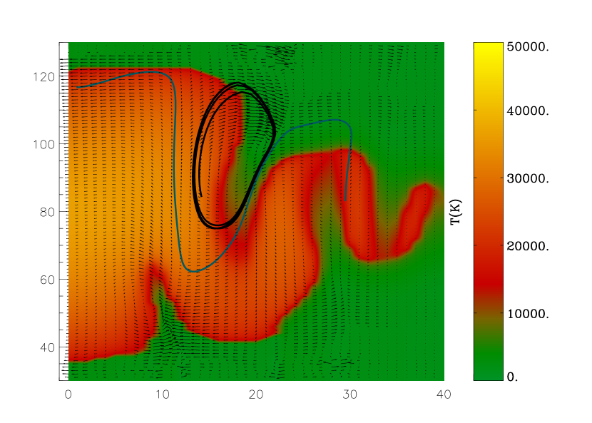
Figure 11: The velocity vectors of the computational grid are plotted on top of the temperature contours at the TI active region. The black and blue curves are the traces of two test particles which are originally placed at the midplane at 0.4 and 0.8 AU.

Figure 11 shows a velocity map of the convective eddies in region (2). We study them by inserting trace particles. These particles rise up with the hot ’red’ fingers which are in the TI high state. When they approach the surface, they enter the region which is cool, dense and in the TI low state. Then they fall with the cool ’green’ fingers to the midplane where they will be heated up again. The convective velocity can be estimated by assuming the particles in the red fingers are accelerated by the buoyancy force from the surrounding dense green fingers. Consider the red fingers are in TI high state with T$\sim$20,000 K and $\rho_{r}$, while the green fingers are in TI low state with T$\sim$2,000 K and $\rho_{g}\sim 10\rho_{r}$. Thus, in the rest frame of the green fingers

$$v_{r}\sim\left(\frac{H_{e}a}{2}\right)^{1/2}\sim\left(\frac{H_{e}g_{h}}{2}\frac{\rho_{g}-\rho_{r}}{\rho_{r}}\right)^{1/2}\sim\left(4.5H_{e}g_{h}\right)^{1/2}$$ (35)

where $H_{e}$ is height of the eddy. $g_{h}$=GM_∗/R³$\times$H/2. While the velocity of the red fingers in the rest frame of the green fingers is

$$v_{g}\sim\left(\frac{H_{e}g_{h}}{2}\frac{\rho_{g}-\rho_{r}}{\rho_{g}}\right)\sim\left(0.5Hg_{h}\right)\,$$ (36)

The real eddy velocity should between v_g and v_r. If H/R$\sim$0.1, $H_{e}$=0.5 H and R=0.2 AU, we derive v${}_{g}\sim$2.3 km s^-1 and v${}_{r}\sim$ 7.1 km s^-1. Thus the average eddy velocity should be around 4 km s^-1. The maximum velocity should not be larger than twice the average velocity. The lower left panel shows the velocity of these eddies, whose velocity is around 4 km s^-1. The maximum velocity takes place at the surface. Although convection is subsonic at the midplane, it is supersonic at the surface (lower right panel in Fig. 10).

3) At $R<0.15\rm AU$ most of the region is already in the TI high state with $T>2\times 10^{4}\rm K$. Thus $(1+\gamma)/(4-\beta)\sim 0.3$, which is similar to the numerical simulation. The surface region where the high state joins to the low state is, however, still convectively unstable (refer to Fig. 9 which shows $\nabla_{S}$ is very large at the transition). Unfortunately our simulation barely resolves this region.

Generally, convection in our simulation is strongly correlated with TI (which is not surprising, since both are related to steep gradients in the opacity). In the outer region where the TI is inactive, convection is weak and inefficient. When the TI is active, the convection patterns depend on the vertical height of the point where hydrogen begins to ionize. If this transition is close to the midplane, convection is strong and penetrates the midplane. Otherwise, only the surface is affected by convection.

5 Discussion

Using our adopted parameters, our 2D simulations produce outbursts which are similar to FU Orionis outbursts, with comparable maximum mass accretion rates ($\sim 2\times 10^{-4}\rm M_{\odot}\,yr^{-1}$) and decay timescales ($\sim 100$yrs). The outbursts begin with the GI transferring mass to the inner disk until it is hot enough to activate the MRI; at that point the disk accretes at a much higher mass accretion rate because of the much higher efficiency of the MRI in transferring angular momentum.

Our outburst scenario is similar to that of Armitage et al. (2001). However, their outbursts were at a much lower mass accretion rate, $\sim 10^{-5}\rm M_{\odot}\,yr^{-1}$, and lasted a longer time, $\sim 10^{4}$ yr. As discovered by Book & Hartmann (2001) and explained in Zhu et al. (2009), their weaker and slower outbursts are due to their lower MRI trigger temperatures ($T_{M}\sim 800\rm K$) and smaller $\alpha_{M}=0.01$. Specifically, with a lower $T_{M}$, the MRI is triggered at a larger radius with a lower surface density, resulting in less mass accumulation in the inner disk. Combined with a smaller $\alpha$, this results in a lower mass loss rate and a longer viscous timescale.

Our choice of $T_{M}\sim 1200\rm K$ is close to the temperature range at which dust is expected to sublimate. This suggests that the mechanism for turn-on of the MRI thermally may be controlled by the elimination of the small dust grains that effectively absorb electrons and thus quench the MRI.

Our radiative transfer modeling of FU Ori (Zhu et al. 2007) suggested that to fit the Spitzer Space Telescope IRS spectrum, the rapidly-accreting, hot inner disk must extend out to $\sim 1$ AU, inconsistent with a pure thermal instability model (Bell & Lin, 1994). In our 2D results we find MRI triggering at about 2 AU, much more consistent with the Spitzer data and our previous analysis in Zhu et al. 2009. As FU Ori has a smaller estimated central star mass (0.3 M_⊙) than the 1 M_⊙ used in our simulations, its hot inner disk should be slightly smaller than derived here, but still in agreement with observations.

Non-Keplerian rotation has not been observed from optical to near-IR (5$\mu$m) lines (Zhu et al., 2009) since these lines come from inner disk within 1 AU where the disk is not massive. However, due to the fact that the disk is massive and gravitationally unstable at large radii (¿2 AU), the disk has slightly sub-Keplerian rotation there and this effect may be observable in the far-IR or submm (Lodato & Bertin, 2003).

We cannot calculate meaningful optical (B magnitude) light curves for comparison with the historical observations of FU Ori objects because our inner disk radius is too large; this results in our maximum effective temperatures being too low in comparison with observations. (This constraint was due to the very long computation times required during outburst; moving the inner radius inward greatly lengthens the computing time.) We therefore computed a 1$\mu$m light curve as a prediction to compare with future observations (Fig. 13), assuming that the disk radiates like a blackbody at each radius’s effective temperature; the lower panel shows the disk’s surface and central temperature at 0.06 AU. The outburst has rise time $\sim$ 10 years, which is similar to V 1515 Cyg but longer than FU Ori. The thermal instability is triggered on a much shorter timescale: as the lower panel shows, the disk’s central temperature rises sharply within 1 year. However, since the mass at the inner disk is still low, the mass accretion rate and the effective temperature cannot increase significantly until the MRI transfers more mass from the outer disk to the inner disk on a viscous timescale. Overall, our simulation agrees with V 1515 Cyg reasonably well but has a longer rise time than FU Ori and V 1057 Cyg. This might be improved by using a smaller inner radius, a consistent central mass, and a self-consistent boundary condition (Kley & Lin, 1999).

Our simulation suggests that the short-timescale variations appearing in the light curves of FU Ori (Kenyon et al., 2000) might be caused by convection in the high state to low state transition region. The observations show $\Delta M\simeq 0.035$ and timescales of less than one day. The amplitude of the variability in the 2D models is $\Delta M\sim 0.2$ (see Fig. 13). In 3D the amplitude of the variability will be reduced because there will be several convective eddies at each radius and averaging over these will reduce the variability. If we assume that the azimuthal extent of a convective eddy is $\sim H$, then there will be $m=2\pi R/H$ convective eddies and the variability will be reduced by a factor of $m^{1/2}\sim 5$ if $H/R\sim 0.2$, suggesting a variability of $\Delta M\sim 0.04$. This agreement the data is encouraging, but it is likely that the details of convection in a magnetized, three dimensional disk will be different from that found in our viscous, axisymmetric models. The modest success of our model, however, might motivate the development of energetically self-consistent 3D magnetohydrodynamical (MHD) models of the inner disk of FU Ori.

The timescale of variability in our 2D models (months) is much longer than the observed 1 day. The timescale of variability might be shortened by (1) increased resolution, since the timescale of variability in our models increases with resolution; (2) switching off all components of stress in Equation 4 except the r-$\Phi$ component, since the other components act to retard and smooth convection (3) replacing the viscosity model used here by MHD turbulence, since the viscosity tends to suppress small scale structure; (4) 3D effects, since one might expect to see variability on timescales of $2\pi/(m\Omega)\sim 1$ day, using $R=0.2\rm AU$ and our estimate for $m$ from above. Overall, although convective behavior revealed by our current simulations are very preliminary (they depend on the simulation resolution, opacity, details of the turbulence etc.), it seems reasonable that convection accounts for the short-timescale variability of FU Orionis objects.

Hartmann, Hinkle, & Calvet (2004) found that some mildly supersonic turbulence ($\sim$ 2 c_s) was needed to explain the width of ¹²CO first-overtone lines of FU Ori . High resolution spectral modeling suggests that CO lines broadened with $\sim$4 km/s turbulent velocity fit the observations well (Zhu et al. 2007). Hartmann, Hinkle, & Calvet (2004) proposed that the MRI could be a mechanism to drive the supersonic turbulence, while here we suggest that convection could also drive the turbulence. Convection is subsonic at the midplane in the TI high state, but as the convective eddies travel to the surface the temperature drops and convection becomes supersonic (see the lower right panel of Fig. 10). Numerical simulations (lower left panel of Fig. 10) and the simple analytical estimate (Eq. 36) suggest the 5 km s^-1 is a typical convective velocity.

We also studied the disk central temperature at the stage when the MRI is activated and then moves inwards. The transition between the TI active and inactive region is sharp and occurs over a radial interval comparable to the disk scale height. The fronts travel at 2.7 $\rm{\,km\,s^{-1}}$, which is almost the sound speed at T = 1000 K. This thermal front velocity is much higher than $\alpha c_{s}$ predicted by Lin et al. (1985) and we will discuss this phenomenon in detail in our next parameter study paper. Notice that in our model the stress is assumed to respond instantaneously to a change in the temperature caused by the radial energy diffusion ; this may indeed be the case if magnetic field mixes into the newly heated gas from the hot side of the transition front. If the magnetic field takes longer than $\sim\Omega^{-1}$ to build up then the front will travel more slowly.

Radiation pressure starts to become significant during the TI high state, with P_r/P${}_{t}\sim$ 0.3 in the innermost regions. We have conducted some experiments including radiation pressure using the diffusion approximation and find generally similar behavior to what has been shown in this paper, though the disk is slightly thicker with the inclusion of radiation pressure. Again, we note that our inner radius is considerably larger than those of T Tauri stars, so radiation pressure might be more important as accreting material joins the central star.

6 Conclusions

We have studied the time evolution of FU Orionis outbursts in a layered disk scenario, using an axisymmetric two dimensional viscous hydrodynamics code with radiative transfer. Both the MRI and GI are considered as angular momentum transport mechanisms and are modeled by a phenomenological $\alpha$ prescription. Besides the surface of the disk ionized by cosmic rays and X-rays, the MRI is also considered to be active as long as the disk’s temperature is above a critical temperature $T_{M}$, so that thermal ionization can provide enough ions to couple the plasma to the magnetic field.

Starting with a massive disk equivalent to a constant $\alpha$ disk with $\dot{M}$=10^-4 M_⊙/yr and $\alpha$=0.1, several outbursts appear during our simulation. These outbursts begin with the GI transferring mass to the inner disk until the inner disk gradually becomes gravitationally unstable. Eventually the disk at 2 AU is hot enough to trigger the MRI and then the MRI active region expands throughout the whole inner disk. With the increasing temperature since the MRI is transferring more mass to the inner disk, the TI is triggered and a “high state” expands outwards to 0.3 AU. The outburst state lasts for hundreds of years and drains the inner disk; the disk then returns to the low state.

Convection appears at the inner disk during the TI high state. In the outer region ($0.35<R<0.6\rm AU$), where the TI is inactive, convection is weak and inefficient. At 0.15¡R¡0.35 $\rm AU$ during outburst, there is a hydrogen ionization zone at $z\sim H$, and strong convection is present. The convection even penetrates the midplane to form antisymmetric convective rolls. In the innermost region most of the disk is hot, the hydrogen ionization zone is close to the photosphere, and weak convection is confined to the disk surface.

Our model shows maximum accretion rates and outburst duration timescales similar to those of the known FU Orionis objects. Unlike the pure TI theory, our model produces an AU scale inner disk with high mass accretion rate, in agreement with the observational constraints.

With some simple assumptions our simulations have produced FU Orionis-like outbursts. They also pose some interesting questions for future study. In a later paper we will compare our 2-D results to 1-D simulations; the latter will allow us to consider longer disk evolutionary timescales.

A dynamical GI simulation at AU scale, with both self-gravity and radiation, will be important to understand angular momentum transport by GI and the thermal structure of the inner disk. However, considering the large Keplerian velocity of the inner disk, a self-consistent radiation hydrodynamic scheme will be needed. Our simulations have also shown that convection is important in FU Orionis objects due to the large vertical temperature gradient at the hydrogen ionization zone. A fully 3-D simulation with both MHD and radiation, together with a self-consistent treatment of the equation of state, will be essential to understanding the role of convection. Also the very inner disk where the MRI is thermally activated by the irradiation and the boundary layer may also play a role in the disk evolution.

Z. Zhu wants to thank Dr. R. Durisen and K. Cai for the inspiring discussion about their radiative transport scheme. This work was supported in part by NASA grant NNX08A139G, by the University of Michigan, and by a Sony Faculty Fellowship, a Richard and Margaret Romano Professorial Scholarship, and a University Scholar appointment to CG. JCM was supported by NASA’s Chandra Fellowship PF7-80048.

7 Appendix A: Radiative cooling scheme tests

To test the radiative transfer scheme (and particularly the boundary condition at the disk photosphere), we have constructed a disk model in which the viscous heating is turned off when $\tau<100$. This makes the vertical flux constant for $\tau<100$ and allows us to test our scheme against a gray atmosphere model. The disk structure shown here is that calculated with Method 1 as discussed in §2.2. The structure calculated with Method 2 is even in a better agreement than Method 1, since it directly uses the gray atmosphere structure as the boundary condition.

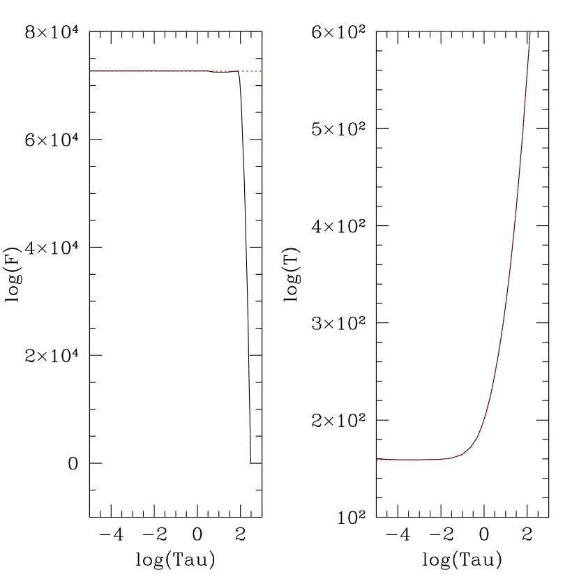
Figure 14: In this test, when $\tau<100$, the viscous heating (2D) is turned off so that the flux is a constant there and can be compared with the gray atmosphere structure. The left panel shows the flux through the atmosphere at different heights, while the dotted line is $F=\sigma T_{eff}^{4}$. The right panel shows the disk temperature structure at one radius from the 2D simulation (solid line) and the theoretical gray atmosphere temperature structure (T⁴=3/4 T${}_{eff}^{4}$($\tau$+2/3) (dotted line).

The left panel in Figure 14 shows the flux through the atmosphere at different heights for one radius, while the dotted line is $F=\sigma T_{eff}^{4}$ with T_eff derived from the simulation. The right panel shows the disk temperature structure at this radius from the 2D simulation (solid line) and the theoretical gray atmosphere temperature structure (T⁴=3/4 T${}_{eff}^{4}$($\tau$+2/3) (dotted line). The vertical structure in the 2D simulation agrees well with the gray atmosphere structure, and improves on the original scheme of Cai et al. (2008) by eliminating a temperature jump at the photosphere.

8 Appendix B: Thermal instability

The thermal instability (TI) model was developed to account for outbursts in dwarf novae systems (Faulkner, Lin, & Papaloizou 1983). But it also has features that make it attractive for explaining FU Ori outbursts (Bell & Lin, 1994). Although in this paper we find that MRI triggering is mainly responsible for initiating FU Orionis outbursts, the TI still exists and can be triggered during the outburst. With the increasing mass accretion rate by the MRI operating, the innermost disk is heated up to hydrogen ionization and the disk becomes thermally unstable. Finally, TI sets in and the innermost disk enter a high (fully ionized) state.

The basic idea behind the TI can be illustrated by the disk $\Sigma-T_{c}$ relationship (’S’ curve, Fig.12). The disk is in thermal equilibrium on this curve. To the left of the curve cooling exceeds heating and to the right heating exceeds cooling. As the disk central temperature reaches $3000\rm K$ the disk transitions from the low-state lower branch to the high-state ($T_{c}\sim 2\times 10^{4}\rm K$) upper branch; it cannot sit on the unstable middle branch.

8.1 ’S’ curve of 2D models

As discussed in §4.1, the LVMZ method (Zhu et al., 2009) produces similar vertical structure to our 2D models. Here, we use the LVMZ to calculate the disk’s $\Sigma-T_{c}$ relation at 0.1 AU in Figure 12. The solid line is the equilibrium curve, while the crosses show $\Sigma$ and $T_{c}$ at 0.1 AU during 2D simulations; the disk moves from the lower left to the upper right with time. The crosses trace the LVMZ curve remarkably well. Since the LVMZ assumes the local cooling through surface balances local viscous heating, it follows that 2D effects, such as radial transport of heat, are not important in this region.

8.2 ’S’ curve of 1D models

In one zone model, where the midplane opacity is used at all $z$ and the total surface density replaces $\rho(z)$, the ’S’ curve can be obtained via

$$F_{vis}=F_{rad}\,.$$ (37)

Thus,

$$\frac{9}{4}\alpha\Omega\Sigma c_{s}^{2}=2\sigma T_{eff}^{4}\,,$$ (38)

where $\Sigma$ is the surface density and $c_{s}$ is the sound speed at the local central disk. For an optically-thick disk, we have T${}_{c}^{4}$=$\frac{3}{8}$$\tau_{R}$T${}_{eff}^{4}$, where $\tau_{R}$=$\kappa_{R}$$\Sigma$ and $\kappa_{R}$ is the Rosseland mean opacity (Hubeny, 1990). Then,

$$T_{c}^{3}=\frac{27}{64\mu\sigma}\alpha\Omega\Sigma^{2}{\cal{R}}_{c}\kappa_{R}\,,$$ (39)

where $\cal{R}$_c is the gas constant, and $\mu$ is the mean molecular weight . This $T_{c}$ and $\Sigma$ relationship is shown in Figure 12, which differs significantly from the LVMZ ’S’ curve.

These ’S’ curves again make the point that the observed large outer radius, 0.5 $-$ 1 AU, of the high accretion rate portion of the FU Ori disk poses difficulties for the pure thermal instability model. Even in the situation explored by Lodato & Clarke (2004), in which the thermal instability is triggered by a massive planet in the inner disk, the outer radius of the high state is still the same as in Bell & Lin (1994), $\sim$ 20 $\rm R_{\odot}$. The relatively high temperatures ($2-4\times 10^{3}$ K) required to trigger the thermal instability (due to the ionization of hydrogen) are difficult to achieve at large radii; they require large surface densities which in turn produce large optical depths, trapping the radiation internally and making the central temperature much higher than the surface (effective) temperature.

Figure 4: The distribution of the vertically integrated surface density at four corresponding stages as shown Figure 2. The long dashed line is the stage before the outburst, while the short dashed line represents the stage when the MRI is triggered at 2 AU. The dotted line shows the moment when the TI is triggered. Finally, the solid line shows the TI fully active stage.

Figure 5: Similar to Figure 4 but shows the effective temperature distribution at the four stages. The long dashed line is the stage before the outburst, while the short dashed line represents the stage when the MRI is triggered at 2 AU. The dotted line shows the moment when the TI is triggered. The solid line shows the TI fully active stage, while the uppermost solid line shows the effective temperature of a steady accretion disk with $\dot{M}\sim$2$\times$10${}^{-4}\rm M_{\odot}\,yr^{-1}$ and R${}_{in}\sim$5$R_{\odot}$

Figure 7: The first three panels show the disk’s mass accretion rate for half-disk models with different inner radius (0.3 AU to 0.06 AU). The lower right panel shows the disk’s mass accretion rate for a full disk with the inner radius 0.06 AU. The red lines are the mass accretion rates after being smoothed.

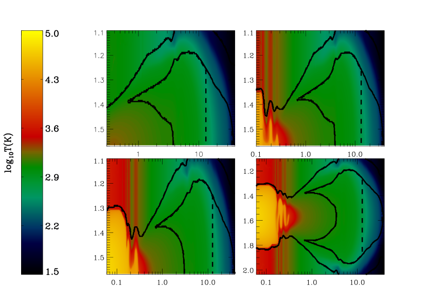
Figure 8: The temperature contours at the stage when their mass accretion rates reach maximum for the four models shown in Figure 7.

Figure 9: The disk’s vertical structure at 0.1 AU in the TI active stage. The crosses are from the 2D simulation grids, while the dotted lines are the disk structure at the same central temperature calculated by the LVMZ method.

Figure 12: The ’S’ curve calculated by the LVMZ (solid curve) and the midplane approximation (dotted curve) at 0.1 AU. The crosses trace the $\Sigma$ and T_c from the 2D simulation.

Figure 13: The solid curve shows the 1$\mu$m magnitude derived from the 2D disk at the beginning of the outburst. The dashed curve in the upper panel shows the mass accretion rate, while the dashed and dotted curves in the lower panel show the midplane and surface temperature at 0.06 AU respectively.

Table 1: 2D models

Labels	inner radius (AU)	half or full disk	resolution
A	0.3	half	80 $\times$ 112
B	0.3	half	160 $\times$ 112
C	0.3	half	320 $\times$ 112
D	0.1	half	80 $\times$ 128
E	0.1	half	160 $\times$ 112
F	0.1	half	324 $\times$ 112
G	0.1	half	576 $\times$ 112
H	0.06	half	304 $\times$ 112
I	0.06	half	512 $\times$ 112
J	0.06	full	128 $\times$ 240
K	0.06	full	320 $\times$ 224

References

- Armitage et al. (2001) Armitage, P. J., Livio, M., & Pringle, J. E. 2001, MNRAS, 324, 705
- Balbus & Papaloizou (1999) Balbus, S. A., & Papaloizou, J. C. B. 1999, ApJ, 521, 650
- Bell & Lin (1994) Bell, K. R., & Lin, D. N. C. 1994, ApJ, 427, 987
- Boley et al. (2006) Boley, A. C., Mejía, A. C., Durisen, R. H., Cai, K., Pickett, M. K., & D’Alessio, P. 2006, ApJ, 651, 517
- Bonnell & Bastien (1992) Bonnell, I., & Bastien, P. 1992, ApJ, 401, 654
- Boss (2002) Boss, A. P. 2002, ApJ, 576, 462
- Cai et al. (2008) Cai, K., Durisen, R. H., Boley, A. C., Pickett, M. K., & Mejía, A. C. 2008, ApJ, 673, 1138
- Cossins et al. (2009) Cossins, P., Lodato, G., & Clarke, C. J. 2009, MNRAS, 393, 1157
- Fromang et al. (2007) Fromang, S., Papaloizou, J., Lesur, G., & Heinemann, T. 2007, A&A, 476
- Gammie (2001) Gammie, C. F. 2001, ApJ, 553, 174
- Green et al. (2006) Green, J. D., Hartmann, L., Calvet, N., Watson, D. M., Ibrahimov, M., Furlan, E., Sargent, B., & Forrest, W. J. 2006, ApJ, 648, 1099
- Guan & Gammie (2008) Guan, X., & Gammie, C. F. 2008, ApJS, 174, 145
- Hartmann et al. (1998) Hartmann, L., Calvet, N., Gullbring, E., & D’Alessio, P. 1998, ApJ, 495, 385
- Hartmann et al. (2004) Hartmann, L., Hinkle, K., & Calvet, N. 2004, ApJ, 609, 906
- h (1985) Hartmann, L., & Kenyon, S. J. 1985, ApJ, 299, 462
- h (1987) Hartmann, L., & Kenyon, S. J. 1987a, ApJ, 312, 243
- h (1987) Hartmann, L., & Kenyon, S. J. 1987b, ApJ, 312, 243
- Hartmann & Kenyon (1996) Hartmann, L., & Kenyon, S. J. 1996, ARA&A, 34, 207
- Herbig (1977) Herbig, G. H. 1977, ApJ, 217, 693
- Hirose et al. (2006) Hirose, S., Krolik, J. H., & Stone, J. M. 2006, ApJ, 640, 901
- Hubeny (1990) Hubeny, I. 1990, ApJ, 351, 632
- Johansen & Levin (2008) Johansen, A., & Levin, Y. 2008, A&A, 490, 501
- Kenyon et al. (1988) Kenyon, S. J., Hartmann, L., & Hewett, R. 1988, ApJ, 325, 231 (KHH88)
- Kenyon et al. (2000) Kenyon, S. J., Kolotilov, E. A., Ibragimov, M. A., & Mattei, J. A. 2000, ApJ, 531, 1028
- King et al. (2007) King, A. R., Pringle, J. E., & Livio, M. 2007, MNRAS, 376, 1740
- Kley & Lin (1999) Kley, W., & Lin, D. N. C. 1999, ApJ, 518, 833
- Lin et al. (1985) Lin, D. N. C., Faulkner, J., & Papaloizou, J. 1985, MNRAS, 212, 105
- Lin & Papaloizou (1980) Lin, D. N. C., & Papaloizou, J. 1980, MNRAS, 191, 37
- Lin & Pringle (1987) Lin, D. N. C., & Pringle, J. E. 1987, MNRAS, 225, 607
- Lodato & Bertin (2003) Lodato, G., & Bertin, G. 2003, A&A, 408, 1015
- Lodato & Clarke (2004) Lodato, G., & Clarke, C. J. 2004, MNRAS, 353, 841
- Lodato & Rice (2004) Lodato, G., & Rice, W. K. M. 2004, MNRAS, 351, 630
- Lodato & Rice (2005) Lodato, G., & Rice, W. K. M. 2005, MNRAS, 358, 1489
- McKinney& Gammie (2002) McKinney, J. C., & Gammie, C. F. 2002, ApJ, 573, 728
- Mihalas & Weibel Mihalas (1984) Mihalas, D., & Weibel Mihalas, B. 1984, New York: Oxford University Press, 1984,
- Miller & Stone (2000) Miller, K. A., & Stone, J. M. 2000, ApJ, 534, 398
- Petrov & Herbig (2008) Petrov, P. P., & Herbig, G. H. 2008, AJ, 136, 676
- Rafikov (2007) Rafikov, R. R. 2007, ApJ, 662, 642
- Ruden et al. (1988) Ruden, S. P., Papaloizou, J. C. B., & Lin, D. N. C. 1988, ApJ, 329, 739
- Stone et al. (1996) Stone, J. M., Hawley, J. F., Gammie, C. F., & Balbus, S. A. 1996, ApJ, 463, 656
- Stone & Norman (1992) Stone, J. M., & Norman, M. L. 1992, ApJS, 80, 753
- Turner & Stone (2001) Turner, N. J., & Stone, J. M. 2001, ApJS, 135, 95
- Vorobyov & Basu (2005) Vorobyov, E. I., & Basu, S. 2005, ApJ, 633, L137
- Vorobyov & Basu (2006) Vorobyov, E. I., & Basu, S. 2006, ApJ, 650, 956
- Whitney et al. (2003) Whitney, B. A., Wood, K., Bjorkman, J. E., & Wolff, M. J. 2003, ApJ, 591, 1049
- Wünsch et al. (2005) Wünsch, R., Klahr, H., & Różyczka, M. 2005, MNRAS, 362, 361
- Zhu et al. (2007) Zhu, Z., Hartmann, L., Calvet, N., Hernandez, J., Muzerolle, J., & Tannirkulam, A.-K. 2007, ApJ, 669, 483
- Zhu et al. (2008) Zhu, Z., Hartmann, L., Calvet, N., Hernandez, J., Tannirkulam, A.-K., & D’Alessio, P. 2008, ApJ, 684, 1281
- Zhu et al. (2009) Zhu, Z., Hartmann, L., & Gammie, C. 2009, ApJ, 694, 1045
- Zhu et al. (2009) Zhu, Z., Espaillat, C., Hinkle, K., Hernandez, J., Hartmann, L., & Calvet, N. 2009, ApJ, 694, L64