THE POINCARÉ SERIES OF THE HYPERBOLIC COXETER GROUPS WITH FINITE VOLUME OF FUNDAMENTAL DOMAINS

Abstract.

The discrete group generated by reflections of the sphere, or Euclidean space, or hyperbolic space are said to be Coxeter groups of, respectively, spherical, or Euclidean, or hyperbolic type. The hyperbolic Coxeter groups are said to be (quasi-)Lannér if the tiles covering the space are of finite volume and all (resp. some of them) are compact. For any Coxeter group stratified by the length of its elements, the Poincaré series (a.k.a. growth function) is the generating function of the cardinalities of sets of elements of equal length. Solomon established that, for ANY Coxeter group, its Poincaré series is a rational function with zeros somewhere on the unit circle centered at the origin, and gave a recurrence formula. The explicit expression of the Poincaré series was known for the spherical and Euclidean Coxeter groups, and 3-generated Coxeter groups, and (with mistakes) Lannér groups. Here we give a lucid description of the numerator of the Poincaré series of any Coxeter group, and denominators for each (quasi-)Lannér group, and review the scene. We give an interpretation of some coefficients of the denominator of the Poincaré series. The non-real poles behave as in Eneström’s theorem (lie in a narrow annulus) though the coefficients of the denominators do not satisfy theorem’s requirements.

1. Introduction

The Coxeter groups split into the three types: spherical, Euclidean, and hyperbolic. These groups are discrete reflection groups acting on, respectively, the sphere, Euclidean space, and Lobachevsky (or hyperbolic) space. If a hyperbolic group divides the space into simplexes of finite volume, it is said to be of Lannér type if it acts cocompactly, and of quasi-Lannér type otherwise. Vinberg suggested the term in honor of Lannér [La] who was the first, it seems (see also [CW]), to list all connected Lannér diagrams (i.e., Coxeter diagrams of Lannér type groups); Shwartsman and Vinberg [VSh] listed all quasi-Lannér diagrams.

Except for the spherical Coxeter groups $I_{2}^{(m)}$ (for $m\neq 3,4,6$), $H_{3}$, and $H_{4}$, each spherical (resp. Euclidean) Coxeter group serves as the Weyl group $W_{{\mathfrak{g}}(A)}$ of simple finite dimensional (resp. affine Kac-Moody) Lie algebra. The hyperbolic groups of (quasi-)Lannér type serve as the Weyl groups of what we suggest to call almost affine Lie algebra ${\mathfrak{g}}(A)$, where $A$ is a Cartan matrix; for the list of almost affine Lie algebras, see the arXiv version of [CCLL]. We assume that all Cartan and Coxeter matrices are indecomposable, unless otherwise stated.

1.1. The three known facts and related problems.

The Poincaré series of the Coxeter groups of spherical and Euclidean types were known. In this paper we explicitly compute the Poincaré series of certain particular Coxeter groups of hyperbolic types.

Fact 1. Among the Coxeter groups $$W W C W_{{\mathfrak{g}}(A)}$$, the eigenvalues of the Coxeter transformation of lie on the unit circle centered at the origin only for spherical or Euclidean groups ([St]). For the Coxeter groups of spherical and Euclidean types, the zeros of the Poincaré series are described in terms of the above mentioned eigenvalues, or rather their exponents, see Table 7.2. (1.1)

Our results show that for the (quasi-)Lannér groups (and, most probably for all hyperbolic Coxeter groups), the zeros of the Poincaré series (which, as we will show, are easy to compute) have nothing to do with the eigenvalues of the Coxeter transformation (which, moreover, are not easy to describe in these cases, see [St]).

Fact 2. The Poincaré series $$W(t) (W,S) S W(t) C C$$ is a rational function for ANY infinite Coxeter group with finite set of generators . The zeros of lie on on the unit circle centered at the origin, but their precise values are known only in the spherical and Euclidean cases. How to determine the precise values of zeros in the other cases was unknown. The Poincaré series of the Coxeter groups of hyperbolic type is exponential, so there is a pole outside and this is all that was known about the poles in general. (1.2)

In [So, Ste, Bou], a somewhat implicit recurrence expression (3.14) for $W(t)$ is given. From [So, Ste, Bou] nothing is clear about the zeros of the denominators. For the Coxeter groups of other than spherical and Euclidean types, the eigenvalues of the Coxeter transformations do not lie on $C$. We show that, nevertheless,

the zeros of the Poincaré series are easy to describe if these functions are represented in a special — virgin — form.

Serre [Se] was, perhaps, the first to observe several patterns in the behavior and properties of the Poincaré series of the spherical Coxeter groups:

1. the Poincaré series are reciprocal;

2. the value of the Poincaré series at $1$ is equal to the inverse of the Euler characteristic of the (geometric realization) of the respective Coxeter group.

In works by M. Davis et. al.([DDJO, DDJMO]) the whole Poincaré series, not only its value at a point, is interpreted in terms of the weighted cohomology of Coxeter groups.

The initial goal of this note was to give an explicit expression not only of the zeros of these rational functions (and try to compare them with the eigenvalues of the Coxeter transformations) but also of their poles (not spoken about in [So, Ste, Bou] at all) in the particular cases of the (quasi-)Lannér groups, i.e., Coxeter groups $(W,S)$ with (quasi-)Lannér Coxeter diagrams. These groups are special in the set of all Coxeter groups, being most close, in a sense, to the Coxeter groups of spherical and Euclidean type: a given Coxeter group is (quasi-)Lannér if its Coxeter diagram is connected, neither spherical nor Euclidean, but any its connected proper subdiagram is spherical (resp. spherical or Euclidean).

Knowing a recurrence formula, the problem does not seem to be difficult ideologically but how to be sure that the result is correct? Our own mistakes we made at first, and those we found in the literature, make this question more serious than we thought at first.

For the case of Coxeter diagrams with 3 vertices, see the paper by Wagreich [Wa]. Wagreich’s paper is very appealing; it also discusses several applications (e.g., due to J. Milnor and M. Gromov) giving motivation for this type of activity and reasons to publish its results in a physical journal. For applications of Poincaré series of the Coxeter groups of spherical or Euclidean type in the theory of simple finite groups, see [So]. There are other types of applications of the Poincaré series of the hyperbolic groups, see, e.g., [BC, GNa, DDJO].

For the Lannér diagrams with 4 and 5 vertices, the answers are known [Wo], and we used them to double check our results. We found out that, for 5 vertices, 3 of 5 Worthington’s answers are wrong. To check our results, we need the correct results of Worthington [Wo], and so we reproduce them. References on Poincaré series of Coxeter groups include [ChD, FP, Fl, Har, Pa1, Pa2, Par], still there is left a room to say something reasonable.

It seemed that the denominators of the Poincaré series of Lannér groups do not admit a nice description (and the situation with quasi-Lannér groups is even worse):

Fact 3. “With the exception of a single real pair of poles, the poles of the Poincaré series of any compact hyperbolic (Lannér) group with $$4 C 5$$ generators lie on the unit circle . This is not so for all -generator Lannér groups” ([CW]). (1.3)

Taking the above facts into account we see the following problems:

(1):

Give reliable criteria for verification of the answers.

(2):

Explicitly describe the poles of the Poincaré series of the 5-generator Lannér groups.

(3):

Explicitly describe the poles of the Poincaré series of quasi-Lannér groups.

(4):

For an infinite Coxeter group $W$, let $e(W)$, called the growth exponent, be the inverse of the radius of convergence $R(W)$ of the Poincaré series $W(t)$. Compute $e(W)$, cf. [Fl].

1.1.1. Our results.

We give an explicit form of the Poincaré series (a.k.a. growth functions) of the Lannér groups (see Tables 7.3 – 7.5) and quasi-Lannér groups (see Tables 7.6 – 7.20).

We offer reliable means for verifications of the correctness of the Poincaré series we list.

We give an interpretation of the highest and the second highest coefficients of the denominator of the Poincaré series in terms of infinite special Coxeter subgroups $W_{X}$ of $W$. Let $D$ be the set of vertices corresponding to the Coxeter diagram of of the group $W$, and $X$ run over all subsets of $D$ such that the special subgroup $W_{X}$ is infinite. We say that a subgroup $W_{J}$ of the Coxeter group $(W,S)$ is special (cf. [Br], p. 26) if it is generated by a subset $J\subset S$. The following statements hold:

Theorem (Theorem on the highest coefficient (Theorem 5.4.1.   Theorem, $1)$).

For any infinite special Coxeter group, the coefficient $b_{n}$ of the highest term of the denominator of the Poincaré series $W(t)$ is as follows:

$$b_{n}=(-1)^{|D|+1}-\sum\limits_{|W_{X}|=\infty}(-1)^{|X|}.$$

Theorem (Theorem on the second highest coefficient (Theorem 5.4.3.   Theorem)).

Let $m$ be the number of factors $[n_{i}]$ in the $[n]$-complete form of the numerator of the the Poincaré series $W(t)$, see §5.4.2. Then the coefficient $b_{n-1}$ of the second highest term of the denominator is as follows:

$$b_{n-1}-mb_{n}=(-1)^{|D|}|D|+\sum\limits_{|W_{X}|=\infty}(-1)^{|X|}|X|.$$

We derive from these theorems the following

Corollary (On the Coxeter group with a single infinite special subgroup (Corollary 5.4.5.   Corollary)).

$1)$ For any Coxeter group with a single infinite special subgroup, we have:

$$b_{n}=0,\quad\text{ and }\quad b_{n-1}\neq 0.$$

In this case, $\deg R-\deg S=1$.

$2)$ For any quasi-Lannér group (and also for any $1$-terminal Coxeter group), the difference of degrees of the numerator and denominator of the Poincaré series is $\deg R-\deg S\leq 1$.

For the Euler characteristics, we have the following statement:

Proposition (On the Euler characteristics (Proposition 5.2.1.   Proposition)).

The Euler characteristics $\chi(W)$ of the group $W$ vanishes (equivalently, the denominator of the Poincaré series has the root $t=1$) in the following cases:

$1)$ For any affine Coxeter group.

$2)$ For any infinite (non-affine) Coxeter group $(W,S)$ with $|S|$ even. (Of course, this case includes (quasi-)Lannér groups whose Coxeter diagrams have even number of vertices.)

We have found out that the poles of the Poincaré series of the quasi-Lannér groups behave rather nicely:

1.2. Towards a generalization of the Eneström theorem.

1.2.1. Gal’s formulation.

For recent studies of the poles of the Poincaré series of Coxeter groups, see Gal’s interesting preprint [Gal] with preliminary results of an aborted research. Gal considered Coxeter diagrams for which the nerve $N_{W}$ (see subsec. 5.5) of the corresponding Coxeter group $W$ is a homology sphere.

Gal wondered how many real poles can the Poincaré series of such a group have (he notes that the degree of the denominator of the Poincaré series of any non-right-angled Coxeter group may be however greater than the dimension of its nerve). If $W$ is an affine Coxeter group, then there is a unique real pole of order $n$ at $1$ [Bou]. If $\dim N_{W}=n\leq 3$, then there are exactly $n$ positive real poles [Par]. Moreover, in these two cases, all the non-real poles lie on the unit circle.

Gal writes that usually (but does not explain what the share of this “usually” in the general picture is and what the exceptions are), if $\dim N_{W}\geq 3$, the non-real poles of the Poincaré series fail to lie on the unit circle. Looking at the examples known to him Gal made the following observation (he writes that he “tested a number of groups whose nerve is a simplex or a product of simplexes” but, regrettably, did not specify the number and gave only two illustrations which, actually, are $L5_{5}$ and $QL10_{2}$):

several poles lie “near”the real positive half-line and the rest of the poles tend to lie “near”the unit circle. (1.4)

We do not know how to quickly say if the nerve of $W$ is a homologic sphere or not, but the examples Gal gives made us wonder if not just two but ALL the cases we study satisfy (1.4). Indeed, they are, with several corrections of Gal’s description:

1.2.2. Quasi-Lannér case. General hyperbolic Coxeter groups.

Having found the precise expressions of the Poincaré series and their poles we saw that the distribution of poles, which could have been random, does resemble the pattern (1.4) almost correctly described by Gal [Gal]. Let us forget for a moment the poles lying “near the real positive half-line”; the remaining poles do lie in a thin annulus concentric with and sometimes containing the unit circle.

Our results and Gal’s hints lead us to a result of G. Eneström [E]. His theorem (rediscovered by Kakeya [Kak], see interesting reviews [GH, vV] and references therein; Kakeya’s work had some mistakes but, despite this, the statement is often referred to as Eneström-Kakeya theorem) says

Theorem.

Let $p(t)=a_{0}+a_{1}t+\dots+a_{n}t^{n}$ be a polynomial with positive coefficients, set $m:=\mathop{\min}\limits_{0\leq i<n}\frac{a_{i}}{a_{i+1}}$, and $M:=\mathop{\max}\limits_{0\leq i<n}\frac{a_{i}}{a_{i+1}}$. Then all the roots of $p(t)$ lie in an annulus with bounding circles of radius $m$ and $M$ concentric with the unit circle $C$ centered at the origin.

The coefficients of the denominators of the Poincaré series of the (quasi-)Lannér groups do not satisfy the conditions of the Eneström theorem but the non-real zeros of these polynomials behave as if they do, or almost: all non-real roots lie in an annulus centered at the origin (except that we do not know how to define the radii $m$ and $M$ of the bounding circle from the coefficients and the annulus does not necessarily contain $C$).

It is natural, therefore, to disregard for a moment the real roots and try to find the conditions the coefficients of the denominators of the Poincaré series of the (quasi-)Lannér groups satisfy in order to derive a generalization of the Eneström theorem for polynomials whose real coefficients can be of any sign or vanish.

At our request, V. Molotkov studied several simplest Lannér cases and saw that the poles lying on $C$ are hardly roots of unity (unlike the zeros of the numerators of the Poincaré series of all Coxeter groups). He also observed that, in contradistinction with what is depicted in Gal’s illustration for $QL10_{2}$, none of the non-real poles is lying “near”the real positive half-line “parallel to it”. Instead

the non-real roots lie in a thin annulus concentric with the unit circle $$C 1 -1$$; the real poles (if any) lie near or . (1.5)

Molotkov’s results, more precise than Gal’s, inspired us to verify and sharpen Gal’s conjecture (1.4) as formulated in (1.5); in most cases, NONE of the non-real roots lies on $C$. Bar few exceptions for 4-vertex diagrams, the poles we found numerically are non-simple-looking (for humans) algebraic numbers. Therefore we have summarized the answer by listing only the real roots and the extremal values of the absolute values of the non-real roots, see Tables 7.22–7.29. We conjectured that the non-real poles of the Poincaré series of any Coxeter group $(W,S)$ with $|S|<\infty$ lie in a thin annulus: This was the case with several of the Coxeter groups we unwillingly considered while making typos in the input data. However, we tested the conjecture on the reflective arithmetic Coxeter groups ([VSh], Table in subsect. 2.1) and non-arithmetic Coxeter groups ([VSh], Table in subsect. 3.2) and found out that this conjecture is overoptimistic: Most the non-real poles of the Poincaré series of these Coxeter groups lie in a thin annulus, but not all.

Problem.

What are the conditions on the coefficients of the real polynomial for its non-real roots to lie in a thin annulus? How to describe the radii of the circles that bound the annulus in terms of the coefficients of the polynomial?

1.3. Discussion: Infinite Coxeter groups.

We conclude from the results of the paper that amount and interrelation of infinite special subgroups in the given infinite Coxeter group is very essential and closely related to predicting coefficients of the Poincaré series. This motivated us to divide the set of all infinite Coxeter groups as follows.

1.3.1. $k$-terminal Coxeter groups.

We say that an infinite Coxeter group $W$ is $k$-terminal if the length of any chain of its infinite special subgroups ordered by inclusion is $\leq k$ and at least one chain is of length $k$. Examples:

$$\begin{split}\{\text{0-terminal}&\text{ Coxeter groups}\}=\{\text{affine Coxeter groups}\}\quad\cup\quad\{\text{Lann\'{e}r Coxeter groups}\}\\ \{\text{1-terminal}&\text{ Coxeter groups}\}=\{\text{quasi-Lann\'{e}r Coxeter groups}\}\quad\cup\quad\\ &\{\text{Coxeter groups with all special subgroups finite, affine or Lann\'{e}r}\}\end{split}$$ (1.6)

Let $W$ be any $k$-terminal Coxeter group and $\mathcal{P}(W)$ the poset of all infinite special subgroups of $W$. Let $l(E)$ be the level of an element $E\in\mathcal{P}(W)$ defined so that $l(W)=0$, $l(E)=1$ for any maximal infinite special subgroup, and so on. Denote by ${\rm Inf}_{m}$ the number of infinite special subgroups of level $m$ in the poset $\mathcal{P}(W)$.

1.3.2. Subsets $I^{n}_{i}$ of infinite Coxeter groups.

Set

$I^{F}$ := { finite Coxeter groups },

$I^{0}_{1}$ := { affine Coxeter groups },

$I^{0}_{2}$ := { Lannér Coxeter groups },  $I^{0}=I^{0}_{1}\cup I^{0}_{2}$,

$I^{1}_{1}$ := { quasi-Lannér Coxeter groups } := { $W\mid$ every proper special subgroup of $W^{\prime}\subset W$ is a group from $I^{F}\cup I^{0}_{1}$, and there exists $W^{\prime}\subset W$ such that $W^{\prime}\in I^{0}_{1}$ },

$I^{1}_{2}$ := { $W\mid$ every proper special subgroup $W^{\prime}\subset W$ is a group from $I^{F}\cup I^{0}$, and there exists $W^{\prime}\subset W$ such that $W^{\prime}\in I^{0}_{2}$},  $I^{1}=I^{1}_{1}\cup I^{1}_{2}$,

Let us introduce by induction subsets $I^{n}_{1}$, $I^{n}_{2}$ and $I^{n}$ as follows:

$I^{n}_{1}$ := { $W\mid$ every proper special subgroup $W^{\prime}\subset W$ is a group from $I^{F}\cup(\bigcup\limits_{i=0}^{n-2}I^{i})\cup I^{n-1}_{1}$, and there exists $W^{\prime}\subset W$ such that $W^{\prime}\in I^{n-1}_{1}$ },

$I^{n}_{2}$ := { $W\mid$ every proper special subgroup $W^{\prime}\subset W$ is a group from $I^{F}\cup(\bigcup\limits_{i=0}^{n-1}I^{i})$, and there exists $W^{\prime}\subset W$ such that $W^{\prime}\in I^{n-1}_{2}$ },  $I^{n}=I^{n}_{1}\cup I^{n}_{2}$.

Proposition.

For $n\geq 0$, we have

$1)$ the set $I^{n}$ consists of $n$-terminal Coxeter groups,

$2)$ $I^{n}_{1}\cap I^{n}_{2}=\emptyset$.

The proposition is easy to prove by induction. ∎.

1.3.4. Classification problem.

As the next natural step in the study of infinite Coxeter groups, it seems to us important to describe the set $I^{1}_{2}$, the next after quasi-Lannér Coxeter groups in hierarchy of the $k$-terminal Coxeter groups.

2. Precise setting of the problems

2.1. Generating functions.

Generating functions of graded objects were introduced and studied by Hilbert and Poincaré at more or less the same time. Leaving touchy priority questions aside, Wikipedia informs us:

“A Hilbert-Poincaré series, named after David Hilbert and Henri Poincaré, is an adaptation of the notion of dimension to the context of graded algebraic structures (where the dimension of the entire structure is often infinite). It is a formal power series in one indeterminate, say $$t t^{n} n$$, where the coefficient of gives the dimension (or rank) of the sub-structure of elements homogeneous of degree .” (2.7)

Observe that in the above definition certain restrictions are taken for granted: the dimension of each homogeneous component must be finite, and only non-negative components are usually non-zero; “graded” is only assumed to be by means of ${\mathbb{Z}}$; for ${\mathbb{Z}}^{k}$-graded objects (under similar restrictions: The support of the degrees with non-empty components lies in the cone with non-negative coordinates and each component is finite), we get series in several indeterminates, as in [McD, DDJO] and Table 7.2.

In the particular case of Coxeter groups stratified by the length of their elements, instead of the term “Hilbert-Poincaré series” the term Poincaré series is usually used, and lately it is called also by the growth function. We use the terminology of the classics, and in a particular case of Coxeter groups of (quasi-)Lannér type is the object of our study.

2.2. Coxeter groups.

A Coxeter system to be a pair $(W,S)$ consisting of a group $W$ and a set of generators $S\subset W$ subject to relations

$$(st)^{m_{s,t}}=1,\text{ where }m_{s,s}=1,m_{s,t}=m_{t,s}\geq 2\text{ for }s\neq t\text{ in }S.$$ (2.8)

If no relation occurs for a pair $s,t$, then it is assumed that $m_{s,t}=\infty$. In this presentation $W$ is a Coxeter group. The symmetric matrix $M=(m_{s,t})_{s,t\in S}$ is called a Coxeter matrix.

The presentation of every finitely generated Coxeter group can be illustrated by an undirected labeled graph, called Coxeter diagram, whose vertices correspond to the generators $S$ of $W$ and edges are as follows. If $m_{s,t}=2$ then no edge joins $s$ and $t$. If $m_{s,t}=3$, then an edge joins $s$ and $t$. The edge between the vertices corresponding to $s,t\in S$ is endowed with label $m_{s,t}$ if $m_{s,t}>3$.

The Poincaré series $W_{W,S}(t)$ of a group $W$ relative to a finite generating set $S$ is briefly denoted $W(t)$ and defined as follows. For any $g\in W$, define the length $l(g)$ to be the minimum length of all words in $S$ representing $g\neq 1$ and $l(1)=0$. Then

$$W(t):=\sum_{g\in W}t^{l(g)}.$$ (2.9)

2.2.1. Remarks

1) The Coxeter diagrams, so graphic for Weyl groups of finite dimensional and Kac-Moody Lie algebras, are utterly useless if the Coxeter matrix is not sparse, as is the case of Lorentzian Lie algebras considered by Borcherds, and Gritsenko and Nikulin, see [GN], or in the cases considered in sect. 3.3. In this note, we deal with the cases where graphs are helpful, but the reader should realize that actually we deal with Coxeter matrices.

2) Other notation used (less convenient, we think, if there are many cases of multiple edges): The edge between nodes $s$ and $t$ is often depicted as a multiple one of multiplicity $m_{s,t}-2$, unless $m_{s,t}=\infty$; for $m_{s,t}=\infty$, the edge is usually depicted thick.

For the Lie algebra ${\mathfrak{g}}(A)$ with Cartan matrix $A$ normalized, as usual, so that $A_{ii}=2$, and with non-positive integer off-diagonal elements, the Coxeter matrix $M=(m_{ij})_{ij\in S}$ is given by the conditions

$$A_{ij}A_{ji}$$ 0 1 2 3

2 3 4 6

(2.10)

We do not reproduce the list of spherical (resp. Euclidean) Coxeter diagrams (see [Vi]): They are easily obtained from the well-known Dynkin graphs and their Cartan matrices, see [Bou], (resp. from their extended versions, see [K, St]).

2.3. Exponents.

Let $W$ be a finite group generated by reflections $r_{i}$, where $i=1,\ldots,n$, in the Euclidean space or, equivalently, on the sphere. (For example, the Weyl group $W=W_{{\mathfrak{g}}}$ of a simple Lie algebra ${\mathfrak{g}}$ naturally acts in the root space of ${\mathfrak{g}}$.) Let ${\bf C}:=\prod r_{i}$ be the product of all generators (in any order; all these products are conjugate, see [St]). For the Weyl groups of simple finite dimensional and affine Kac-Moody Lie algebras, the eigenvalues of ${\bf C}$ are of the form $\omega^{m_{i}}$, where $\omega=e^{2\pi i/h}$ and where $h=1+\max m_{i}$ is the Coxeter number — the order of ${\bf C}$ ([CM], [OV], [St]). The numbers $m_{i}$ are called the exponents of the corresponding Coxeter group, see [Cox, Table 2], and our Table 7.1.

Here is an excerpt from [Cox, p.765] regarding exponents (at places in our own words):

“Most of the applications of $${\bf C} h \omega^{m_{1}},\ldots,\omega^{m_{n}} {\bf C} 0 h m_{ij} (m_{l}+1)(m_{2}+1)\ldots(m_{n}+1), m_{i}+1 n m_{ij} G G (1+t^{2m_{l}+1})(1+t^{2m_{2}+1})\ldots(1+t^{2m_{n}+1})."$$ are related with . We consider the characteristic roots of and the exponents are certain integers which may be taken to lie between and . They are computed by a trigonometrical formula involving the periods [i.e., orders] of the products of pairs of generators. (The product of two reflections is simply a rotation.) The point of interest is that the same integers occur in a different connection. It turns out that the order of the group is and that these factors are the degrees of basic invariant forms [William Burnside, Theory of Groups of Finite Order, Cambridge, 1911; Chapter XVII]. Moreover, when every is equal to 2, 3, 4 or 6, so that the group is crystallographic, there is a corresponding continuous group , and the Betti numbers of the group manifold are the coefficients in the Poincaré polynomial (of the manifold of the Lie group )

2.4. The Poincaré series (a.k.a. growth functions) of the Coxeter groups.

Following Solomon, Bourbaki [Bou] gives an explicit expression of the Poincaré series $W_{{\mathfrak{g}}}(t)$ for the Weyl group $W_{{\mathfrak{g}}}$ of simple finite dimensional Lie algebra ${\mathfrak{g}}$ in terms of exponents:

$$W_{{\mathfrak{g}}}(t)=\prod\frac{1-t^{m_{i}+1}}{1-t}.$$ (2.12)

This formula is applicable not only to the Weyl groups of the simple finite dimensional Lie algebras, but to other groups of spherical type, see Table 7.2.

The generalization of (2.12) to affine Weyl groups is due to Bott [Bo]; see also Reiner’s notes [Rei] with an exposition of the proof of Bott’s result due to Steinberg [Ste]. Bott keeps writing about the loop groups or loop algebras (i.e., algebras of the form $\tilde{\mathfrak{g}}:={\mathfrak{g}}\otimes{\mathbb{C}}[u^{-1},u]$, where ${\mathfrak{g}}$ is any simple finite dimensional Lie algebra), but in reality he only considers the Weyl groups of the Lie algebras of these loop groups. Since the exponents are defined up to dualization of the root system, the Poincaré series for the “twisted” affine Kac-Moody algebras are covered by Bott’s result. The answer is given by the formula

$$W_{\tilde{\mathfrak{g}}}(t)=\prod\frac{1-t^{m_{i}+1}}{(1-t)(1-t^{m_{i}})}=W_{{\mathfrak{g}}}(t)\prod\frac{1}{1-t^{m_{i}}}.$$ (2.13)

Let us now try to perform the next step — consider the Weyl groups of almost affine Lie algebras.

2.5. Digression: (Quasi-)Lannér groups are the Weyl groups of almost affine Lie algebras.

There are several (intersecting but distinct) sets of Lie algebras whose elements are often called “hyperbolic” Lie algebras. We would like to carefully distinguish between these sets so need an appropriate name for each. We say that a submatrix of a square matrix is principal if it is obtained by striking out a row and column that intersect on the main diagonal. We say that Lie algebra with Cartan matrix whose entries belong to the ground field is almost affine if it is not finite dimensional or affine, and its subalgebra corresponding to any principal submatrix of the Cartan matrix is the sum of finite dimensional or affine Lie algebras.

Z. Kobayashi and J. Morita classified the almost affine Lie algebras with indecomposable symmetrizable Cartan matrix of size $>2$ [KoMo]. Later, Li Wang Lai [Li] obtained a complete answer (for Cartan matrices of size $>2$): there are 238 almost affine Lie algebras; 142 of these algebras have a symmetrizable Cartan matrix. Later Saçlioğlu [S] rediscovered the result of Kobayashi and Morita (with few omissions); his paper is devoted to physical applications and is very interesting.

In this paper we derive explicit formulas for the Poincaré series of the groups most close in a sense to the Weyl groups of simple finite dimensional Lie algebras. In the literature, in similar studies, the authors write sometimes that they are studying the Lie algebras or even the Lie groups having these Lie algebras, whereas they are only studying the Weyl groups of these Lie algebras. This subtlety is sometimes important: In particular, to list all the groups we are dealing with (Lannér and quasi-Lannér) is much easier than to list the Lie algebras whose Weyl groups they are. These are almost affine (a.k.a hyperbolic) Lie algebras; their complete list was unknown when the description of the growth functions of their Weyl groups has begun (and the classification of these Lie algebras is not needed in this particular study of their Weyl groups). There are several stages of generalization of simple finite dimensional Lie algebras (which all possess very particular Cartan matrices) to the Lie algebras with more-or-less arbitrary Cartan matrix. We intend to generalize the results on the growth functions known for the Weyl groups of simple finite dimensional and affine Kac-Moody Lie algebras to the case of Weyl groups of almost affine Lie algebras. These Lie algebras became of acute interest lately in connection with “cosmic billiards”; for details and further references, see [H], [BS]. The Poincaré series of the Weyl groups of almost affine Lie algebras are invariants of these Lie algebras that can be used further, see [Wa] and references therein. The set of almost affine Lie algebras has a non-empty intersection with the (different) set of Lorentzian Lie algebras, sometimes also called “hyperbolic”. For applications of Lorentzian Lie algebras, see [RU], [GN]. For one of these applications Borcherds was awarded with Fields medal.

3. The Poincaré series (known facts)

3.1. The Solomon-Steinberg recursion (3.14).

For any finite set $X$, let $\varepsilon(X)=(-1)^{\mathop{\mathrm{card}}\nolimits(X)}$. Let $W_{X}(t)$ be the Poincaré series (a polynomial or series) of the Coxeter group $W_{X}$ whose Coxeter graph is $X$. If $\mathop{\mathrm{card}}\nolimits W_{D}<\infty$, let ${\mathcal{M}}$ be the maximal length of the elements of $W_{D}$ (there is only one element of maximal length).

Ex. 26 to §1 of Ch.4 [Bou] claims that for any Coxeter graph $D$, we have (this formula is obviously due to Solomon [So] (although in particular cases of finite Weyl groups this may have been established earlier by Chevalley, see §3.15 in [Hu]); Steinberg [Ste], Theorem 1.25 gave a simpler proof; for an exposition of Steinberg’s proof, see also [McD], where there are considered multiparameter series taking into account difference in length of roots); here $X$ is any complete subgraph of $D$:

$$\sum_{X\subset D}\frac{\varepsilon(X)}{W_{X}(t)}=\begin{cases}\displaystyle\frac{t^{{\mathcal{M}}}}{W_{D}(t)}&\text{if $\mathop{\mathrm{card}}\nolimits W_{D}<\infty$},\\ 0&\text{otherwise}.\end{cases}$$ (3.14)

In this expression, the summand corresponding to the empty subgraph is equal to $1$.

Recall that the rational (non-polynomial) function $P(t)$ is said to be reciprocal if $P(t^{-1})=P(t)$; if $P(t^{-1})=-P(t)$ the rational function $P(t)$ is often said to be anti-reciprocal.

The polynomial function $P(t)$ is said to be reciprocal (resp.anti-reciprocal) if

$$P(t)=t^{{\mathcal{M}}}P(t^{-1}),\text{~{}~{}(resp. $P(t)=-t^{{\mathcal{M}}}P(t^{-1})$), where ${\mathcal{M}}=\deg P$}.$$

The (anti-)reciprocal function is said to be $\pm$-reciprocal.

The recurrence (3.14) and $\pm$-reciprocity of $W_{X}(t)$ if $|W_{X}|<\infty$ imply the following sharpening of (3.14) due to Steinberg [Ste]: If $\mathop{\mathrm{card}}\nolimits W_{D}=\infty$, then

$$\frac{1}{W_{D}(t^{-1})}=\sum_{X\subset D\;\;\mid\;\;\mathop{\mathrm{card}}\nolimits W_{X}<\infty}\frac{\varepsilon(X)}{W_{X}(t)}.$$ (3.15)

To begin the induction, recall the following facts:

0) If the Coxeter graph $X$ is the disjoint union of its connected components $X_{i}$, then $W_{X}(t)=\prod W_{X_{i}}(t)$. Hereafter it is advisable to use standard simplified notation: For any $n\in{\mathbb{N}}\cup\{\infty\}$, set

$$[n]:=\begin{cases}1+t+\dots+t^{n-1}&\text{for $n<\infty$},\\ 1+t+\dots=\displaystyle\frac{1}{1-t}&\text{for $n=\infty$}.\end{cases}$$ (3.16)

1) $W_{\emptyset}(t)=1$ and $W_{*}(t)=1+t=[2]$ (that is, for the graph consisting of 1 vertex and 0 edges).

2) If $X$ has two vertices joined by $m-2$ edges, then

$$W_{X}(t)=\begin{cases}\displaystyle\frac{(1+t)(1-t^{m+2})}{1-t}=[2][m+1]&\text{if $3\leq m<\infty$ (for $I_{2}^{(m)}$)},\\ \displaystyle\frac{1+t}{1-t}=[2][\infty]&\text{if $m=\infty$ (for $I_{2}^{(\infty)}$)}.\end{cases}$$ (3.17)

3) The Poincaré series of the 3-generator Coxeter group $G_{p,q,r}$ with diagram $L3$ or $QL3$ (if $|G_{p,q,r}|<\infty$, then $\frac{1}{p}+\frac{1}{q}+\frac{1}{r}>1$):

$$W_{G_{p,q,r}}(t)=\frac{[2][p][q][r]}{[2][p][q][r]-3[p][q][r]+[p][q]+[p][r]+[q][r]}\times\begin{cases}(t^{\mathcal{M}}+1)&\text{if $|G_{p,q,r}|<\infty$, }\\ 1&\text{otherwise}.\end{cases}$$ (3.18)

The Coxeter graphs are as follows:

$L3$: Each diagrams on 3 vertices is a triangle with edges labeled by $p$, $q$, $r$ such that $2\leq p,q,r<\infty$ and $\frac{1}{p}+\frac{1}{q}+\frac{1}{r}<1$. One (only one) of the labels $p$, $q$, $r$ may be equal to 2, and then the graph is not, actually, a triangle.

$QL3$: The graphs look as those for $L3$ but any of the labels $p$, $q$, $r$ may be (and at least one is) equal to $\infty$.

We summarize the results needed to explicitly compute (3.15) in Table 7.2.

3.2. Lannér and quasi-Lannér diagrams on $>3$ vertices.

In the literature we saw, these diagrams are seldom identified (the only exception known to us is an interesting paper [JKRT] with too complicated names for them), so we simply number them for convenience. The first to list these diagrams was, it seems, Lannér [La], see also [CW50].

For the Lannér diagrams and the corresponding Poincaré series, see Tables 7.3 – 7.5.

For the quasi-Lannér diagrams and the corresponding Poincaré series, see Tables 7.6 – 7.20.

3.2.1. Worthington’s results.

For the Lannér groups with 4 generators, Worthington computed their Poincaré series, and we confirm them in Table 7.3–7.4. Worthington computed the Poincaré series of the quasi-Lannér groups with 5 generators, but in 3 of 5 cases his answers are wrong.

3.3. Two interesting (and correct although strange) — but useless for us — formulas.

Floyd and Plotnick [FP] cite the following statement they attribute to Parry. The first displayed eq. on p.524 of [FP] gives the following presentation of a Coxeter group $W$:

$$W=\left\langle g_{1},\dots,g_{d}\mid g_{i}^{2},(g_{i}g_{i+1})^{a_{i}}\right\rangle.$$ (3.19)

Obviously $i$ runs 1 through $d$ and — although this was not mentioned (sapienti sat) — the relation between $g_{d}$ and $g_{d+1}$ should be understood as a relation between $g_{d}$ and $g_{1}$. Since nothing is mentioned, there are no relations between $g_{i}$ and $g_{j}$ for $i\neq j\pm 1$ (and $g_{d}$ and $g_{j}$ for $j\neq d-1$ or 1), i.e., there are lots of relations of the form $(g_{i}g_{j})^{\infty}=1$. Then (as usual, the hatted factor should be ignored)

$$W(t)=\frac{[2][a_{1}]\dots[a_{n}]}{(t+1-n)[a_{1}]\dots[a_{n}]+\sum[a_{1}]\dots\widehat{[a_{i}]}\dots[a_{n}]}.$$ (3.20)

In 1991, Floyd submitted a paper [Fl] in which the following condition of applicability of formula (3.20) is added to tho conditions given in [FP]: The set $a_{1}$, …, $a_{n}$ is said to be unacceptable if $(a_{1},\dots,a_{n})=(2,2,2,2)$ for $n=4$ or $\frac{1}{a_{1}}+\frac{1}{a_{2}}+\frac{1}{a_{3}}\geq 1$ for $n=3$. For all other — acceptable — sets of labels, the following formula is offered in place of (3.20):

$$W(t)=\frac{[2][a_{1}]\dots[a_{n}]}{[2][a_{1}]\dots[a_{n}]-t\sum[a_{1}]\dots[a_{i}-1]\dots[a_{n}]}.$$ (3.21)

The MAIN applicability condition of (3.20) and (3.21) mentioned in [FP, Fl] is, however, that

the group $$W$$ should act on the 2-dimensional hyperbolic space. (3.22)

The mysterious (how to verify it for an abstractly given group?) condition (3.22) is applicable to the (quasi-)Lannér graphs only in certain cases of three vertices, so it is of no interest to us. We have included the remarkable — they are symmetric in the $a_{i}$ which is astounding — formulas (3.20) and (3.21) in this paper for completeness of the picture.

3.4. The multiparameter case.

Macdonald [McD] describes the passage to the multiparameter case with his usual clarity:

For any Coxeter group $(W,S)$, let $S_{i}$ for a set of indices $I$, be the equivalence classes of the relation “$s$ is conjugate to $s^{\prime}$ in $W$” between elements of $s,s\in S$.

The subsets $$S_{i} (W,S) \infty S_{i}$$ can be read off the Coxeter diagram of the group by “reduction modulo 2”: if we delete from the diagram all bonds bearing the even label or , then the connected components of the resulting graph correspond to the . (3.23)

Let ${\bf t}=(t_{i})_{i\in I}$ be a family of indeterminates. For each $s\in S$, define

$$t_{s}:=t_{i}\text{~{}~{} for $s\in S_{i}$}.$$ (3.24)

Let $w=s_{i_{1}}\dots s_{i_{l}}$ be a reduced decomposition of any $w\in W$, i.e., representation of $w$ as the product of the least number of generators. Then the monomial

$$t_{w}:=t_{s_{i_{1}}}\dots t_{s_{i_{l}}}$$ (3.25)

does not depend on the choice of reduced decomposition. Then, clearly,

$$W({\bf t}):=\sum_{w\in W}t_{w}.$$ (3.26)

Let $l_{i}(w)$ be the $i$-length of $w$, i.e., the number of the generators in the reduced decomposition of $w$ belonging to $S_{i}$. Then

$$t_{w}:=\prod_{i\in I}t_{i}^{l_{i}(w)}.$$ (3.27)

With these definitions, the formula (3.14) is still true with ${\bf t}$ instead of $t$. For the necessary changes, see Table 7.2: For the Coxeter groups of spherical type, $|I|\leq 2$ and $|I|=2$ only in the three cases.

Observe several subtleties:

1) Clearly, the Coxeter diagram $D$ is not sufficient to describe the multiparameter Poincaré series: We have to distinguish between short and long roots if $|D|>2$, so we have to distinguish between the $B_{n}$ and $C_{n}$ cases.

2) Although the Lie algebras with non-symmetrizable Cartan matrices do have the Weyl group defined by eq. (2.10), Macdonald’s rule (3.23) is only applicable to the root systems described by symmetrizable Cartan matrices: Otherwise the notion of short/long root is not well-defined.

Although Macdonald’s paper is devoted to all Coxeter groups of spherical and Euclidean cases, he evaded computing the multiparameter Poincaré series for the Weyl groups of the twisted loop Lie algebras leaving this as “an easy task for the reader”, having indeed explained all the needed steps. This was, perhaps, a joke: all one should do is to renumber the indeterminates in accordance with Table 7.2 minding the above subtlety 1). Macdonald missed (or left as a trivial exercise?) the case of $A_{1}^{(1)}$ (the answer for which coincides with that for $A_{2}^{(2)}$, see Table 7.21).

Unless the authors of [DDJO], where the multiparameter growth functions are applied, or somebody else, will ask us to do the job, we intend to imitate the behavior of Prof. Macdonald, and redirect the reader: For the classification of Li and Saçlioğlu, see more accessible list in [CCLL]; the code is available at [DCh] and how to proceed with the code is described in the last section of this work. The task is now routine while to list the results will double the length of the tables.

4. The Euler characteristic (from [D], [Br])

4.1. The geometric realization of the simplicial complex.

A simplicial complex with vertex set ${\mathcal{V}}$ is a collection $\Delta$ of finite subsets of ${\mathcal{V}}$ (called simplexes) such that every singleton $\{v\}$ is a simplex and every subset of a simplex $A$ is a simplex (called a face of $A$), [Br, Ch.I, App.]. The cardinality $r$ of $A$ is called the rank of $A$, and $r-1$ is called the dimension of $A$. We include the empty set as a simplex; it has rank $0$ and dimension $-1$. A subcomplex of $\Delta$ is a subset $\Delta^{\prime}$ which contains, for each of its elements $A$, all the faces of $A$, thus $\Delta^{\prime}$ is a simplicial complex in its own right, with vertex set equal to some subset of ${\mathcal{V}}$. Note that $A$ is a poset, ordered by the face relation.

The geometric realization $|\Delta|$ of $\Delta$ is a topological space partitioned into (open) simplexes $A$, one for each non-empty $A\in\Delta$. This topological space is constructed as follows: We start with an abstract real vector space with ${\mathcal{V}}$ as a basis. Let $|A|$ be the interior of the simplex in ${\mathcal{V}}$ spanned by the vertices of $A$, i.e., $|A|$ consists of the linear combinations $\sum\limits_{v\in A}{\lambda_{v}}v$ with $\lambda_{v}>0$ for all $v\in A$ and $\sum\limits_{v\in A}{\lambda_{v}}=1$. We then set

$$|\Delta|=\bigcup\limits_{A\in\Delta}|A|.$$

4.2. Cells and chambers.

Let $V$ be the space of a geometric realization of the Coxeter group $(W,S)$, and $\dim V=n$. Let $\mathbb{H}=\{H_{1},...,H_{k}\}$ be an arbitrary finite set of hyperplanes in $V$. The hyperplanes $H_{i}$ cut $V$ into polyhedral pieces by means of reflections $s_{i}:=s_{H_{i}}$ that generate $W$ . For each $i=1,...,k$, where $k=\mathop{\mathrm{card}}\nolimits(S)$, let $f_{i}:V\longrightarrow\mathbb{R}$ be a non-zero homogeneous linear function that singles out $H_{i}$ by the equation $f_{i}=0$. The function $f_{i}$ is uniquely determined by $H_{i}$, up to a non-zero factor.

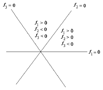
Figure 4.1.   Here $\dim V=2$ and $k=3$. The three lines divide the plane into $13$ cells ($6$ open sectors, $6$ open rays, and the cell consisting of the origin.

1) A cell in $V$ with respect to $\mathbb{H}$ is a non-empty set $A$ obtained by choosing, for each $i$, the half-space $f_{i}>0$ or $f_{i}<0$ or the hyperplane $f_{i}=0$.

2) The cells defined by taking only the $f_{i}$ corresponding to half-spaces are called chambers. Essentially, the chambers can be described as the cells of maximal dimension. Sometimes what we defined here as chambers are called cells in the literature.

3) Chambers are the connected components of the complement

$$V\setminus\bigcup\limits_{i=0}^{k}{H}_{i}.$$ (4.28)

4) Let $C$ be the simplicial cone in $V$ defined by the inequalities

$$f_{i}\geq 0\text{ for }i=1,2,\dots,n.$$ (4.29)

It is called the fundamental chamber.

4.3. The Coxeter complex.

A cell $B$ is said to be a face of $A$ if its description is obtained from that of $A$ by replacing several inequalities by equalities. In this case, we write

$$B\leq A$$ (4.30)

and this relation is said to be face relation. We have

$$\overline{A}=\bigcup\limits_{B\leq A}B,$$

and

$$B\leq A\Longleftrightarrow\overline{B}\subseteq\overline{A}$$ (4.31)

Let $\Sigma$ be the poset consisting of the open cells, ordered by the face relation. By (4.31) $\Sigma$ is isomorphic to the set of closed cells, see [Br, Ch.I].

4.3.1. The simplicial complex $\Sigma(W,S)$.

Let $(W,S)$ be a Coxeter group. Consider the subcomplex $\Sigma_{\leq C}$ consisting of the faces of $C$. With every face $A\leq C$, we associate its stabilizer $W_{A}=\{w\in W\mid wA=A\}$. By a theorem in [Br, Ch.I, §5F], $W_{A}$ is generated by a subset $A\subset S$.

There is a function $\Phi$ from $\Sigma_{\leq C}$ to the set of special subgroups of $W$; this $\Phi$ is a bijection ([Br, Ch.I, §5H]):

$$\Sigma_{\leq C}\approx\text{(special subgroups of $(W,S)$)}^{op},$$ (4.32)

where “op” indicates that we are using the opposite of the usual order on the set of special subgroups.

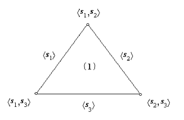
Figure 4.2.   Illustration of the isomorphism (4.32) for $n=3$.

The $W$-action can be used to extend the isomorphism (4.32) to an isomorphism of the whole poset $\Sigma$ with the set of special cosets in $W$, i.e., the cosets $wW^{\prime}$ of special subgroups.

Theorem.

([Br, Ch.I, §5H]) There is a poset isomorphism

$$\Sigma\approx\text{(special cosets of $(W,S)$)}^{op}$$ (4.33)

compatible with the $W$-action on the special cosets by left-translation.

The Theorem Theorem allows one to introduce geometry into abstract group theory. Let $W$ be a group, possibly infinite, generated by a subset $S$ consisting of elements of order 2. Define, a special coset to be a coset $w\langle{S^{\prime}}\rangle$ with $w\in W$ and $S^{\prime}\subset S$. Now define $\Sigma=\Sigma(W,S)$ to be the poset of special cosets, ordered by the opposite of the inclusion relation: $B\leq A$ in $\Sigma$ if and only if $B\supset A$ as subsets of $W$, in which case we say that $B$ is a face of $A$.

Following Tits, $\Sigma$ is called the Coxeter complex associated to $(W,S)$, it is also called the “apartment associated to $(W,S)$”, see [Br02].

4.4. The Euler characteristic.

For any finite simplicial complex, the Euler characteristic is defined as the alternating sum

$$\chi=k_{0}-k_{1}+k_{2}-k_{3}+...,$$

where $k_{n}$ denotes the number of cells of dimension $n$ in the complex.

For any topological space, we can define the $n$th Betti number $b_{n}$ as the rank of the $n$-th singular homology group. The Euler characteristic is then equal to the alternating sum

$$\chi=b_{0}-b_{1}+b_{2}-b_{3}+....$$

This quantity is well-defined if the Betti numbers are all finite and if they are zero beyond a certain index $n_{0}$.

5. The Poincaré series of the Lannér and quasi-Lannér groups (new results)

Having computed something different from Worthington’s results, we realized that means of verification are badly needed. Besides, later we obtained a bit different picture describing distribution of poles than the one Gal gave for $QL10_{2}$. But our goal was not to refute (or verify) somebody’s results but to say something new. At first, we could only say something negative (“there is no reciprocity”, “not all non-real poles lie on the unit circle $C$ centered at the origin”, etc.), which was not appealing. Fortunately, we managed to observe several patterns that one can formulate in a positive way:

1. If the number of vertices of a given quasi-Lannér diagram is even, the Euler characteristic vanishes.

2. The difference of degrees of the numerator and denominator of the Poincaré series is always $\leq 1$ in the quasi-Lannér cases.

3. The virgin form of the Poincaré series is equal to its reduced form in the quasi-Lannér cases bar the following exceptions: $QL4_{8}$, $QL4_{12}$, $QL4_{14}$, $QL4_{15}$, $QL4_{19}$, $QL6_{5}$, $QL6_{9}$, $QL6_{11}$, $QL8_{1}$, $QL8_{2}$, $QL8_{4}$.

In what follows we give a priori proofs of these and several other patterns.

5.1. Reciprocity for the Lannér diagrams

Lemma (On reciprocity).

Let a polynomial $S(t)$ be factorized as follows:

$$S(t)=U(t)V(t),$$

and let $U(t)$ be anti-reciprocal. Then

$$\begin{array}[]{cc}S(t)\text{ is anti-reciprocal if and only if }V(t)\text{ is reciprocal},\\ S(t)\text{ is reciprocal if and only if }V(t)\text{ is anti-reciprocal}.\end{array}$$

Since $t-1$ is an anti-reciprocal polynomial, this rather obvious lemma helps us to understand that denominators of Poincaré series of all Lannér diagrams on $4$ vertices are anti-reciprocal, see Tables 7.3 and 7.4.

Proposition.

$1)$ Let $(W,S)$ be the Coxeter system, such that all special subgroups of $W$ are finite. If $\mathop{\mathrm{card}}\nolimits{S}$ is even, the Poincaré series $W(t)$ is anti-reciprocal. If $\mathop{\mathrm{card}}\nolimits{S}$ is odd, the Poincaré series $W(t)$ is reciprocal.

$2)$ The Poincaré series $W(t)$ of the Lannér groups on $4$ vertices are anti-reciprocal, and the Poincaré series $W(t)$ of the Lannér groups on $5$ vertices are reciprocal.

Proof.

1) By (3.14) and (3.15) we have

$$\begin{array}[]{ccc}&-\displaystyle\frac{\epsilon(D)}{W_{D}(t)}=&\sum\limits_{X\subsetneq D}\displaystyle\frac{\varepsilon(X)}{W_{X}(t)},\\ \\ &\displaystyle\frac{1}{W_{D}(t^{-1})}=&\sum\limits_{|W_{X}|<\infty}\displaystyle\frac{\varepsilon(X)}{W_{X}(t)}.\\ \end{array}$$ (5.34)

Since all special subgroups are finite, then the right hand sides in both equations coincide. Thus, if $|S|$ is even (resp. odd), then $-\epsilon(D)$ is negative (resp. positive) and the Poincaré series is anti-reciprocal (resp. reciprocal).

2) Note, that in the case of Lannér groups,

the set of all finite special subgroups coincides with the set of all special subgroups. (5.35)

Then the statement desired follows from heading 1). ∎

Conjecture.

For the Coxeter groups, the (anti)reciprocity never holds, bar the cases listed in Prop. 5.1.2.   Proposition.

5.2. When does the Euler characteristics vanish?

Proposition.

The Euler characteristics $\chi(W)$ of the group $W$ vanishes (equivalently, the denominator of the Poincaré series has the root $t=1$) in the following cases:

$1)$ For any affine Coxeter group.

$2)$ For any infinite (non-affine) Coxeter group $(W,S)$ with $|S|$ even. (Of course, this case includes (quasi-)Lannér groups whose Coxeter diagrams have even number of vertices.)

Proof.

1) Follows from (2.13).

2) By (5.34), we have

$$-\frac{\epsilon(D)}{W_{D}(t)}=\frac{1}{W_{D}(t^{-1})}.$$

Substituting $t=1$ for $\mathop{\mathrm{card}}\nolimits{D}$ even, we see that

$$-\frac{1}{W_{D}(1)}=\frac{1}{W_{D}(1)},\quad\text{ i.e.,}\quad\frac{1}{W_{D}(1)}=0.$$

For illustration of this fact, see Tables 7.6, 7.7, 7.8, 7.11 and 7.12. ∎

5.2.2. The virgin form of the numerator.

The numerator of $W_{D}(t)$ is equal to the denominator of the sum $\mathop{\sum}\limits_{X\subsetneq D}\frac{\varepsilon(X)}{W_{X}(t)}$. By (2.12), for the finite Coxeter group $W_{X}$ with exponents

$$m_{1},m_{2},\dots,m_{k},$$

the Poincaré series $W_{X}$ is a polynomial of the form

$$[m_{1}+1][m_{2}+1]\dots[m_{k}+1].$$ (5.36)

The least common multiple

$${\rm Virg}(D):=\mathop{{\rm LCM}}\limits_{X\subsetneq D\text{ such that }|W_{X}|<\infty}W_{X}(t)$$ (5.37)

is said to be the virgin form of the numerator of $W_{D}(t)$.

Lemma.

The Poincaré series $W_{D}(t)$ can be expressed as a rational fraction whose numerator is ${\rm Virg}(D)$.

Proof.

The statement is obvious if all special subgroups $W_{X}$ are finite: then the numerator of $W_{D}(t)$ is equal to the denominator of the sum $\mathop{\sum}\limits_{X\subsetneq D}\frac{\varepsilon(X)}{W_{X}(t)}$ and all denominators of its summands are polynomials of the form (3.16). The general case is done by induction on $|X|$. ∎

Corollary.

Let $\displaystyle\frac{\varepsilon(X)}{W_{X}(t)}$ be expressed as an irreducible fraction. Then the LCM of all denominators in the sum $\mathop{\sum}\limits_{X\subsetneq D}\displaystyle\frac{\varepsilon(X)}{W_{X}(t)}$ is equal to ${\rm Virg}(D)$.

Proof.

Indeed, if $|W_{X}|=\infty$, then the denominator of the irreducible fraction $\displaystyle\frac{\varepsilon(X)}{W_{X}(t)}$ divides ${\rm Virg}(X)$ and ${\rm Virg}(X)$ divides ${\rm Virg}(D)$. If $|W_{X}|<\infty$, then $W_{X}(t)$ divides ${\rm Virg}(D)$ by definition. Hence, the LCM of denominators divides ${\rm Virg}(D)$.

Implication in the opposite direction: divisibility of the LCM of denominators by ${\rm Virg}(D)$ is obvious. ∎

If $|W_{X}|<\infty$, then $W_{X}(t)$ is of the form (3.16). We would like to represent ${\rm Virg}(D)$ in the same form, but this is not always possible: if $m$ and $n$ are not relatively prime, then $[m]$ and $[n]$ are not relatively prime. On the other hand, each polynomial $[n]$ can be represented as the product of irreducible over ${\mathbb{Q}}$ cyclotomic polynomials $\Phi_{i}(t)$, where $i=2,3,\dots$, namely

$$[n]=\mathop{\prod}\limits_{i|n,~{}i>1}\Phi_{i}(t).$$ (5.38)

THEREFORE, IT IS NATURAL TO COMPUTE ${\rm Virg}(D)$ IN THE FORM OF THE PRODUCT OF THE $\Phi_{i}(t)$.

It is convenient to introduce one more notation:

$$[n^{\prime}]:=1+t^{n};\text{~{}~{} observe that~{}}[n][n^{\prime}]=[2n].$$ (5.39)

5.3. Degrees of the denominators.

In this section, we define the polynomials $P,Q,R,S$ by setting:

$$W(t):=\frac{R(t)}{S(t)}\text{~{}~{}and ~{}~{}}W(t^{-1}):=\frac{P(t)}{Q(t)}.$$ (5.40)

Proposition.

For any Coxeter group, we have

$1)$ $\deg P=\deg Q$;

$2)$ $\deg S<\deg R$ if and only if $t\mid Q(t)$.

Proof.

1) According to the Solomon formula (2.12), for any finite Coxeter group, every cyclotomic polynomial-factor of $W(t^{-1})$ turns into the fraction

$$\frac{1+t+...+t^{n-1}}{t^{n-1}}$$

For any affine Coxeter group, Proposition follows from (2.13). For any infinite Coxeter group, we use the Steinberg formula (3.15). Recall that $1$ in the numerator above is the summand corresponding to the empty set in (3.15). This summand contributes the maximal degree equal to the degree of the denominator of $W(t^{-1})$. Therefore, $\deg P=\deg Q$.

2) Note that $t\mid Q(t)$ if and only if $a_{0}=0$, where $a_{0}$ is the constant term of $Q(t)$, which becomes the highest coefficient of $S(t)$ under the substitution $t\longmapsto t^{-1}$. Thus, the condition $t\mid Q(t)$ is equivalent to $\deg S<\deg R$. ∎

Proposition.

$1)$ For the function $\epsilon(X)=(-1)^{|X|}$, we have

$$a)\mathop{\sum}\limits_{\emptyset\subseteq X\subseteq D}\epsilon(X)=0,\qquad b)\mathop{\sum}\limits_{\emptyset\subseteq X\subseteq D}\epsilon(X)\,|X|=0.$$ (5.41)

$2)$ We have:

$$\frac{1}{W(t^{-1})|_{t=0}}=\mathop{\sum}\limits_{X\subset D~{}\mid~{}|W_{X}|<\infty}\epsilon(X).$$ (5.42)

$3)$ If $f(t)$ is the product of $k$ factors $[n_{i}]$, then $f^{\prime}(0)=k$.

$$f(t)=\prod\limits_{i=1}^{k}[n_{i}]\quad\Longrightarrow\quad f^{\prime}(0)=k.$$ (5.43)

$4)$ If $|X|<\infty$, then

$$W^{\prime}_{X}(t)\mid_{t=0}=|X|.$$ (5.44)

Proof.

1) Formula (5.41,a) holds since

$$\sum\limits_{\emptyset\subseteq X\subseteq D}\epsilon(X)=\sum\limits_{k=0}^{n}(-1)^{k}\Big{(}\mathchoice{\raisebox{0.25pt}{$\genfrac{}{}{0.0pt}{0}{n}{k}$}}{\raisebox{0.25pt}{$\genfrac{}{}{0.0pt}{0}{n}{k}$}}{\raisebox{-0.5pt}{$\genfrac{}{}{0.0pt}{1}{n}{k}$}}{\raisebox{-0.5pt}{$\genfrac{}{}{0.0pt}{1}{n}{k}$}}\Big{)}=(1-1)^{n}=0,$$

and formula (5.41,b) is true since

$$\sum\limits_{\emptyset\subseteq X\subseteq D}\epsilon(X)\mid X\mid=\sum\limits_{k=0}^{n}(-1)^{k}\Big{(}\mathchoice{\raisebox{0.25pt}{$\genfrac{}{}{0.0pt}{0}{n}{k}$}}{\raisebox{0.25pt}{$\genfrac{}{}{0.0pt}{0}{n}{k}$}}{\raisebox{-0.5pt}{$\genfrac{}{}{0.0pt}{1}{n}{k}$}}{\raisebox{-0.5pt}{$\genfrac{}{}{0.0pt}{1}{n}{k}$}}\Big{)}k=-n\sum\limits_{k=0}^{n}(-1)^{k-1}\Big{(}\mathchoice{\raisebox{0.25pt}{$\genfrac{}{}{0.0pt}{0}{n-1}{k-1}$}}{\raisebox{0.25pt}{$\genfrac{}{}{0.0pt}{0}{n-1}{k-1}$}}{\raisebox{-0.5pt}{$\genfrac{}{}{0.0pt}{1}{n-1}{k-1}$}}{\raisebox{-0.5pt}{$\genfrac{}{}{0.0pt}{1}{n-1}{k-1}$}}\Big{)}=-n(1-1)^{n}=0.$$

2) By the Steinberg formula (3.15) for $\displaystyle\frac{1}{W(t^{-1})}$, every summand of (3.15) is of the form

$$u_{i}(Z)=\frac{\varepsilon(Z)}{[n_{1}][n_{2}]\dots[n_{k}]}$$ (5.45)

Since $[n_{i}]|_{t=0}=1$, we have $u_{i}(Z)=\varepsilon(Z)$.

3) Eq. (5.43) holds since

$$f^{\prime}(t)=\sum\limits_{i=1}^{k}[n_{i}]^{\prime}\prod\limits_{j=1;j\neq i}^{k}[n_{i}],\quad\text{ and }\quad f^{\prime}(0)=\sum\limits_{i=1}^{k}[n_{i}]^{\prime}\mid_{t=0}=\sum\limits_{i=1}^{k}1=k.$$

4) Since the number of factors $[n_{i}]$ in the Poincaré series of any finite Coxeter group is equal to the number of its generators, i.e., to the number of vertices $|X|$, then $\eqref{deriv_2}$ follows from $\eqref{deriv_1}$. ∎

Proposition.

$1)$ The following relation holds:

$$\frac{1}{W(t^{-1})}\Big{|}_{t=0}~{}~{}=~{}~{}(-1)^{|D|+1}-\mathop{\sum}\limits_{|W_{X}|=\infty}(-1)^{|X|}.$$ (5.46)

$2)$ For degrees of the numerator and denominator of $W(t)$, we have:

$$\deg S<\deg R\quad\text{ if and only if }\quad\mathop{\sum}\limits_{|W_{X}|=\infty}\varepsilon(X)=\mathop{\sum}\limits_{|W_{X}|=\infty}(-1)^{|X|}=(-1)^{|D|+1}.$$ (5.47)

$3)$ We have:

$$\left(\frac{1}{W(t^{-1})}\right)^{\prime}\Big{|}_{t=0}=\sum\limits_{|W_{X}|=\infty}{(-1)}^{|X|}|X|+{(-1)}^{|D|}|D|.$$ (5.48)

Proof.

1) Follows from the fact that the sum in (5.42) differs from (5.41,a) by summands associated with the infinite special subgroups and the subset $X=D$.

2) According to Proposition 5.3.1.   Proposition the condition $\deg S<\deg R$ is equivalent to $Q(t)=0$, or, in other words, to

$$\frac{1}{W(t^{-1})}\Big{|}_{t=0}=0.$$

Then the statement follows from (5.46).

3) Since

$$\frac{1}{W(t^{-1})}=\sum\limits_{|W_{X}|<\infty}\frac{\varepsilon(X)}{W_{X}(t)},$$

we have

$$\left(\frac{1}{W(t^{-1})}\right)^{\prime}=-\sum\limits_{|W_{X}|<\infty}\frac{W^{\prime}_{X}(t)\varepsilon(X)}{\left(W_{X}(t)\right)^{2}}$$

For any finite Coxeter group, we have $W_{X}(t)|_{t=0}=1$. By (5.44) $W^{\prime}_{X}(t)\Big{|}_{t=0}=|X|$, and we see that

$$\left(\frac{1}{W(t^{-1})}\right)^{\prime}\Big{|}_{t=0}=-\sum\limits_{|W_{X}|<\infty}\varepsilon(X)|X|.$$

According to (5.41,b) we have:

$$\left(\frac{1}{W(t^{-1})}\right)^{\prime}\Big{|}_{t=0}=\sum\limits_{|W_{X}|=\infty}\varepsilon(X)|X|+\varepsilon(D)|D|,$$

and (5.48) holds.

∎

Corollary.

For the quasi-Lannér diagrams, we have $\deg S<\deg R$ only in the following cases:

$$\begin{array}[]{l}QL4_{1},\quad QL4_{2},\quad QL4_{3},\quad QL4_{6},\quad QL4_{8},\quad QL4_{14},\quad QL4_{17},\quad QL4_{18},\quad QL4_{19};\\ QL5_{1},\quad QL5_{2},\quad QL5_{3},\quad QL5_{6},\quad QL5_{7};\\ QL6_{5},\quad QL6_{7},\quad QL6_{10};\\ QL7_{1},\quad QL7_{2},\quad QL7_{3};\\ QL8_{1},\quad QL8_{2},\quad QL8_{3},\quad QL8_{4};\\ QL9_{1},\quad QL9_{2},\quad QL9_{3};\\ QL10_{1}.\\ \end{array}$$ (5.49)

Proof.

Indeed, only in these cases there is a single infinite special subgroup in the given quasi-Lannér Coxeter group.

For diagrams on $4$ vertices, this subgroup is associated with $X$, such that $|X|=3$. Further, $|D|+1=5$, and $(-1)^{|X|}=(-1)^{|D|+1}=-1$. Then, the statement follows from (5.47). The cases of $>4$ vertices are absolutely analogous. ∎

5.4. The coefficients $b_{n}$ and $b_{n-1}$ of the denominator.

Let $b_{n}$ (resp. $b_{n-1}$) be the coefficient corresponding the degree $n$ (resp. $n-1$) of the denominator of Poincaré series $W(t)$. Consider

$$\frac{1}{W(t^{-1})}=\frac{Q(t)}{P(t)},\text{ where }Q(t)=\sum\limits_{i=0}^{n}{a}_{i}{t}^{i},\quad P(t)=\prod\limits_{i=1}^{m}[n_{i}].$$ (5.50)

We have:

$$a_{0}=b_{n},\qquad a_{1}=b_{n-1}.$$ (5.51)

Now, we will prove two theorems predicting values of coefficients $b_{n}$ and $b_{n-1}$ of the denominator. It is clear that the other coefficients $b_{i}$ of the denominator can be predicted in the same way. Note that calculations of $b_{n}$ and $b_{n-1}$ are closely connected with the poset of infinite special subgroups in $W$. The following theorem is devoted to the coefficient $b_{n}$. Actually, the conclusion (5.47) is a particular case of this theorem.

Theorem.

All Poincaré series in the tables are normalized so that $b_{n}=1$.

$1)$ For the coefficient $b_{n}$ of the highest term of the denominator $S(t)$ of $W(t)$, we have

$$b_{n}=(-1)^{|D|+1}-\sum\limits_{|W_{X}|=\infty}(-1)^{|X|}\quad.$$ (5.52)

$2)$ For any $0$-terminal Coxeter group, in particular, for any Lannér group, we have

$$b_{n}=(-1)^{|D|+1},$$ (5.53)

see Tables 7.3, 7.4, 7.5.

$3)$ For any $1$-terminal Coxeter group $W$, in particular, for any quasi-Lannér group, we have

$$b_{n}=(-1)^{|D|}({\rm Inf}-1),\quad{\rm Inf}=b_{n}+1,$$ (5.54)

where ${\rm Inf}$ is the number of infinite special subgroups in $W$, see Tables 7.6 – 7.20.

$4)$ For any $k$-terminal Coxeter group $W$, we have

$$b_{n}=(-1)^{|D|+1}\sum\limits_{i=0}^{m}{(-1)^{m}{\rm Inf}_{m}},$$ (5.55)

Proof.

1) Recall that by (5.40) $P(t)$ (resp. $Q(t)$) is the numerator (resp. denominator) of $W(t^{-1})$. The case $P(t)=0$ is considered in Theorem 5.3.3.   Proposition. Now, let $P(t)\neq 0$. Since

$$Q(t)=\prod\limits_{i=1}^{k}[n_{i}],$$

we have $Q(0)=1$. Thus,

$$\frac{1}{W(t^{-1})}\Big{|}_{t=0}=P(0)=a_{0}\neq 0,$$

where $a_{0}$ is the constant term of the denominator $P(t)$ of $W(t^{-1})$. Substitution $t\longmapsto t^{-1}$ turns $a_{0}$ into $b_{n}$, the coefficient of the highest term of the denominator $R(t)$ of $W(t)$.

2) For Lannér groups (and also $0$-terminal) the term $\sum\limits_{|W_{X}|=\infty}(-1)^{|X|}$ in (5.52) vanishes.

3) For quasi-Lannér (and $1$-terminal) groups we have $|D|=|X|+1$, where $X$ is the subdiagram corresponding any infinite subgroups, and (5.54) holds. ∎

5.4.2. The $[n]$-complete and reduced forms of the Poincaré series

The following theorem is devoted to predicting the coefficient $b_{n-1}$ of the denominator of the Poincaré series. The calculation of $b_{n-1}$ is based on the parameter $m$ of the numerator meaning the number of factors like $[n_{i}]$ in the numerator. However, the numerator which we consider is not mandatory irreducible. If it contains a divisor of some $[n_{i}]$, we multiply the numerator and denominator to get only factors like $[n_{i}]$. This non-irreducible form of the the Poincaré series is said to be the $[n]$-complete form. Thus, our prediction is related to the numerator of the $[n]$-complete form. Note that

(1) For the quasi-Lannér Coxeter groups, there are only two cases, namely $QL8_{1}$ and $QL8_{2}$, with two $[n]$-incomplete factors. In the cases $QL4_{8}$, $QL4_{12}$, $QL4_{14}$, $QL4_{15}$, $QL4_{19}$, $QL6_{5}$, $QL6_{9}$, $QL6_{11}$, $QL8_{4}$, there is only one $[n]$-incomplete factor. In the remaining cases the $[n]$-complete form and reduced form coincide.

(2) The following fact holds: after reduction of the $[n]$-complete form of the Poincaré series for Lannér and quasi-Lannér groups the number of factors $m$ is not changed. None of the factors $[n_{i}]$ is completely reduced.

(3) The difference of degrees of the numerator and denominator $\deg R-\deg S$ does not change under reduction. This fact allows us to calculate $\deg R-\deg S$ for the $[n]$-complete form and to apply it to the reduced form.

Theorem.

Let $m$ be the number of factors $[n_{i}]$ in the $[n]$-complete form as (5.50). Then

$$b_{n-1}-mb_{n}=\sum\limits_{|W_{X}|=\infty}(-1)^{|X|}|X|+(-1)^{|D|}|D|.$$ (5.56)

Proof.

Since

$$\left(\frac{1}{W(t^{-1})}\right)^{\prime}\Big{|}_{t=0}\quad=\quad\frac{f^{\prime}(t)g(t)-f(t)g^{\prime}(t)}{(g(t))^{2}}\Big{|}_{t=0},\text{ and }g(0)=1,$$

and by (5.43) $g^{\prime}(0)=m$, we have

$$\left(\frac{1}{W(t^{-1})}\right)^{\prime}\Big{|}_{t=0}\quad=\quad f^{\prime}(0)-f(0)g^{\prime}(0)\quad=\quad a_{1}-m{a}_{0}.$$

By (5.51),

$$\left(\frac{1}{W(t^{-1})}\right)^{\prime}\Big{|}_{t=0}\quad=\quad b_{n-1}-m{b}_{n}.$$

Then eq. (5.56) follows from (5.48). ∎

Corollary.

For any Lannér group we have:

$$\begin{split}&b_{n}=-1,\quad b_{n-1}=1\quad\text{ for }\quad L4_{i},\quad 1\leq i\leq 9,\\ &b_{n}=1,\quad b_{n-1}=-1\quad\text{ for }\quad L5_{i},\quad i=1,3,4,\\ &b_{n}=1,\quad b_{n-1}=0\quad\text{ for }\quad L5_{i},\quad i=2,5.\end{split}$$ (5.57)

Remark.

Eq. (5.57) holds for the $[n]$-complete form, and does not hold for the reduced form, see Tables 7.3, 7.4, 7.5. All Poincaré series in Tables 7.3, 7.4, 7.5 are normalized so that $b_{n}=1$.

Proof.

Since Lannér groups does not contain infinite subgroups, i.e., ${\rm Inf}=0$, then $b_{n}=(-1)^{|D|+1}$, see (5.53).

For $|D|=4$, the number of factors $m=3$. In this case, by (5.56) we have

$$b_{n-1}=mb_{n}+(-1)^{|D|}|D|=3(-1)+4=1.$$

For $|D|=5$, the number of factors $m=4$ (except for $L5_{2}$ and $L5_{5}$). In this case, by (5.56) we have

$$b_{n-1}=mb_{n}+(-1)^{|D|}|D|=4-5=1.$$

For $|D|=5$, cases $L5_{2}$ and $L5_{5}$, the number of factors $m=5$. In this case, by (5.56) we have

$$b_{n-1}=mb_{n}+(-1)^{|D|}|D|=5-5=0.$$

∎

Corollary.

$1)$ For any Coxeter group with a single infinite subgroup, we have:

$$b_{n}=0,\quad\text{ and }\quad b_{n-1}\neq 0.$$ (5.58)

In this case, $\deg R-\deg S=1$.

$2)$ For any quasi-Lannér group (and also for any $1$-terminal Coxeter group), the difference of degrees of the numerator and denominator of the Poincaré series is $\deg R-\deg S\leq 1$.

Proof.

1) According to (5.56), and since ${\rm Inf}=1$, we have

$$b_{n-1}-mb_{n}=(-1)^{|X|}|X|+(-1)^{|D|}|D|,$$

where $|X|=|D|-1$, i.e.,

$$b_{n-1}-mb_{n}=(-1)^{|X|}(|X|-|X|+1|)=(-1)^{|X|},$$

From (5.54) we have $b_{n}=0$, and therefore $b_{n-1}=(-1)^{|X|}$, so (5.58) holds.

2) Let $b_{n}=0$. Since in the case of $1$-terminal Coxeter group $|X|+1=|D|$ for all infinite subgroups $X\subset D$, all summands ${(-1)}^{|X|}$ in (5.52) have the same sign. Since $b_{n}=0$, there exists only one infinite special subgroup, and by 1) we have $\deg R-\deg S=1$. ∎

Conjecture.

For ANY infinite Coxeter group, $\deg R-\deg S\leq 1$.

Corollary.

Any infinite Coxeter group having exactly two infinite special subgroups is $1$-terminal or $2$-terminal.

$1)$ For any $1$-terminal Coxeter group with exactly two infinite special subgroups, we have:

$$b_{n}={(-1)}^{|D|},\quad\text{ and }\quad b_{n-1}={(-1)}^{|D|}(m+2-|D|).$$ (5.59)

$2)$ The quasi-Lannér groups with exactly two infinite special subgroups are as follows:

a) For $|D|=4$, $m=3$, we have $b_{n}=1,b_{n-1}=1$, (see cases $QL4_{4}$, $QL4_{7}$, $QL4_{11}$, $QL4_{12}$).

b) For $|D|=4$, $m=2$, we have $b_{n}=1,b_{n-1}=0$, (see cases $QL4_{5}$, $QL4_{10}$, $QL4_{21}$).

c) For $|D|=5$, $m=4$, we have $b_{n}=-1,b_{n-1}=-1$, (see case $QL5_{8})$.

d) For $|D|=6$, $m=5$, we have $b_{n}=1,b_{n-1}=1$, (see cases $QL6_{1}$, $QL6_{3}$, $QL6_{11}$).

e) For $|D|=9$, $m=8$, we have $b_{n}=-1,b_{n-1}=-1$, (see case $QL9_{4}$).

f) For $|D|=10$, $m=9$, we have $b_{n}=1,b_{n-1}=1$, (see case $QL10_{2}$).

$3)$ For any $2$-terminal Coxeter group with exactly two infinite special subgroups, we have

$$b_{n}={(-1)}^{|D|+1},\quad\text{ and }\quad b_{n-1}={(-1)}^{|D|+1}(m+1-|D|).$$ (5.60)

Proof.

Follows from (5.52) and (5.56). ∎

5.5. Nerves and geometric realization of the group.

From [ChD, p.374]: The nerve of $(W,S)$, denoted by $N$, is the poset of subsets $X\subset S$ for which the group $W_{X}:=(W,X)$ is finite. The poset is ordered with respect inclusion. The proper nerve of $(W,S)$ is the poset $N_{>\emptyset}$ consisting of the nonempty subsets $X\subset S$ such that $W_{X}$ is finite.

Clearly, $N_{>\emptyset}$ is a simplicial complex. More precisely, it is isomorphic to the poset of simplices of a simplicial complex with vertex set $S$. (For more facts and explanations, see subsect. 4.3.)

For any finite poset $K$, let $\chi(K)$ denote the Euler characteristic of its geometric realization (see subsect. 4.1, 4.4). The following formula due to Serre [Se] connects the Poincaré series of a given Coxeter group and its Euler characteristic:

$$\frac{1}{W(1)}=\chi(W)\qquad\text{({\bf The Serre Formula})}.$$ (5.61)

6. The code to compute the Poincaré series and means of control

To compute the Poincaré series, we used the Mathematica-based code subg due to D. Chapovalov [DCh] and double-checked with a code due to R. Stekolshchik.

6.1. Code subg.

We rewrite the expression (3.14) in the following form

$$W_{D}(t)=\frac{-\varepsilon(D)}{\mathop{\sum}\limits_{X\subsetneq D}\frac{\varepsilon(X)}{W_{X}(t)}}.$$ (6.62)

This formula enables one to express the Poincaré series $W_{D}(t)$ in terms of the finite groups listed in Table 1. The corresponding recursion was automatically generated by the code subg. The format and notation (improving Coxeter symbols) are designed so that each step can be easily verified by a human, and, on the other hand, these intermediate results can be copied to Mathematica in order to derive the final answer.

6.2. Poles.

Having found the Poincaré series we determined their poles by means of Mathematica and Molotkov verified our findings with the help of the code pari, see [rf].

Acknowledgements.

We are thankful to R. Grigorchuk, P. de la Harpe, B. Okun, O.  Shwartsman, and É.  Vinberg for useful comments. We are thankful to A. Chapovalov and D. Chapovalov, and to V. Molotkov for invaluable help in computing.

7. Tables

Table 7.1.  The exponents, Coxeter number, and the maximal length of the elements in the spherical Coxeter groups with connected Coxeter diagram

Coxeter	Lie	exponents	maximal length	Coxeter
group	algebra	$m_{i}$	$l(w_{0})=\sum m_{i}$	number $h$
$A_{n}$	${\mathfrak{sl}}(n+1)$	$1,2,3,\dots,n$	$\displaystyle\frac{n(n+1)}{2}$	$n+1$
$B_{n}$	${\mathfrak{o}}(2n)$ for $n\geq 2$	$1,3,\dots,2n-1$	$n^{2}$	$2n$
$C_{n}$	${\mathfrak{sp}}(2n)$ for $n\geq 2$	$1,3,\dots,2n-1$	$n^{2}$	$2n$
$D_{n}$	${\mathfrak{o}}(2n+1)$	$1,3,\dots,2n-3;\;n-1$	$n(n-1)$	$2(n-1)$
$G_{2}$	${\mathfrak{g}}_{2}$	$1,5$	$6$	$6$
$F_{4}$	${\mathfrak{f}}_{4}$	$1,5,7,11$	$24$	$12$
$E_{6}$	${\mathfrak{e}}_{6}$	$1,4,5,7,8,11$	$36$	$12$
$E_{7}$	${\mathfrak{e}}_{7}$	$1,5,7,9,11,13,17$	$63$	$18$
$E_{8}$	${\mathfrak{e}}_{8}$	$1,7,11,13,17,19,23,29$	$120$	$30$
$I_{2}^{(m)}$ for $m>6$	—	$1,m-1$	$m$	$m$
or $m=5$
$H_{3}$	—	$1,5,9$	$15$	$10$
$H_{4}$	—	$1,11,19,29$	$60$	$30$

Note. The groups $I_{2}^{(m)}$ are the non-crystallographic dihedral groups for $m=5$ and $m>6$. For $m=3,4,\text{ and }6$, respectively, we have the crystallographic dihedral group as follows:

$$A_{2}=I_{2}^{(3)},\qquad B_{2}=C_{2}=I_{2}^{(4)},\qquad G_{2}=I_{2}^{(6)}.$$

Table 7.2.  The Poincaré series of the spherical Coxeter groups with connected Coxeter diagram

Coxeter group	its Poincaré series
$A_{n}$	$[2]\dots[n+1]$
$B_{n}$	$[2]\dots[2n]$
$D_{n}$	$[2]\dots[2n-2][n]$
$G_{2}$	$[2][6]$
$F_{4}$	$[2][6][8][12]$
$E_{6}$	$[2][5][6][8][9][12]$
$E_{7}$	$[2][6][8][10][12][14][18]$
$E_{8}$	$[2][8][12][14][18][20][24][30]$
$I_{2}^{(m)}$ for $5\leq m\leq\infty$	$[2][m]$
$H_{3}$	$[2][6][10]$
$H_{4}$	$[2][12][20][30]$
Coxeter group	multiparameter Poincaré series ($u:=t_{1}t_{2}$)
$I_{2}^{(m)}$ for $6\leq m=2k\leq\infty$	$(1+t_{1})(1+t_{2})\begin{cases}\frac{1-u^{m}}{1-u}&\text{if $m<\infty$}\\ \frac{1}{1-u}&\text{if $m=\infty$}\end{cases}$
$F_{4}$	$\left(\mathop{\prod}\limits_{j=1,2}(1+t_{j})(1+t_{j}+t_{j}^{2})(1+ut_{j})\right)\mathop{\prod}\limits_{i=1}^{3}(1+u^{i})$
$B_{n}$ ($t_{2}$ corr. to the short root)	$\mathop{\prod}\limits_{i=0}^{n-1}(1+t_{1}^{i}t_{2})(1+t_{1}+\dots+t_{1}^{i})$
$C_{n}$ ($t_{2}$ corr. to the long root)	$\mathop{\prod}\limits_{i=0}^{n-1}(1+t_{1}^{i}t_{2})(1+t_{1}+\dots+t_{1}^{i})$

Table 7.3.  The Lannér diagrams on $4$ vertices and Poincaré series

Label	Diagram	Poincaré series
	Degrees	$\chi=0$ in all cases
$L4_{1}$		$\displaystyle\frac{[2][6][10]}{t^{15}-t^{14}-t^{11}+t^{4}+t-1}=$
	$(11,11)$
		$\displaystyle\frac{[2][6][5^{\prime}]}{t^{11}-2t^{10}+t^{9}-t^{7}+2t^{6}-2t^{5}+t^{4}-t^{2}+2t-1}$
$L4_{2}$		The numerator is $[4][6][10]$
	$(15,15)$	The denominator is
		$t^{17}-t^{16}+t^{15}-2t^{14}+t^{13}-2t^{12}+t^{11}-t^{10}$
		$+t^{9}-t^{8}+t^{7}-t^{6}+2t^{5}-t^{4}+2t^{3}-t^{2}+t-1$
		Can be reduced to the numerator: $[4][10][3^{\prime}]$
		and denominator: $t^{15}-2t^{14}+2t^{13}-2t^{12}+t^{11}-t^{10}$
		$+t^{9}-t^{8}+t^{7}-t^{6}+t^{5}-t^{4}+2t^{3}-2t^{2}+2t-1$
$L4_{3}$		$\displaystyle\frac{[2][6][10]}{t^{15}-t^{14}-t^{12}-t^{9}+t^{8}-t^{7}+t^{6}+t^{3}+t-1}=$
	$(13,13)$
		$\displaystyle\frac{[2][10](1+t^{3})}{t^{13}-2t^{12}+t^{11}-t^{9}+t^{8}-t^{7}+t^{6}-t^{5}+t^{4}-t^{2}+2t-1}$
$L4_{4}$		The numerator is $[4][6][10]$
	$(11,11)$	The denominator is
		$t^{17}-t^{16}+t^{15}-2t^{14}+t^{13}-3t^{12}+2t^{11}$
		$-3t^{10}+3t^{9}-3t^{8}+3t^{7}-2t^{6}+3t^{5}-t^{4}+2t^{3}-t^{2}+t-1$
		Can be reduced to
		$\displaystyle\frac{[4][3^{\prime}][5^{\prime}]}{t^{11}-3t^{10}+4t^{9}-4t^{8}+3t^{7}-2t^{6}+2t^{5}-3t^{4}+4t^{3}-4t^{2}+3t-1}$
$L4_{5}$		$\displaystyle\frac{[2][4][6]}{t^{9}-t^{8}-t^{7}+t^{2}+t-1}=$
	$(7,7)$
		$\displaystyle\frac{[2][4][3^{\prime}]}{t^{7}-2t^{6}+2t^{4}-2t^{3}+2t-1}$

Table 7.4.  The Lannér diagrams on $4$ vertices and Poincaré series (cont.)

Label	Diagram	Poincaré series
	Degrees	$\chi=0$ in all cases
$L4_{6}$		$\displaystyle\frac{[4][6][10]}{t^{17}-t^{16}-t^{14}-t^{13}-t^{12}-t^{11}+t^{6}+t^{5}+t^{4}+t^{3}+t-1}$
	$(17,17)$
		Can be reduced to:
	$(11,11)$	$\displaystyle\frac{[4][3^{\prime}][5^{\prime}]}{t^{11}-3t^{10}+3t^{9}-t^{8}-2t^{7}+4t^{6}-4t^{5}+2t^{4}+t^{3}-3t^{2}+3t-1}$
$L4_{7}$		$\displaystyle\frac{[2][4][6]}{t^{9}-t^{8}-t^{7}-t^{6}+t^{3}+t^{2}+t-1}$
	$(9,9)$
		Can be reduced to:
	$(7,7)$	$\displaystyle\frac{[2][4][3^{\prime}]}{t^{7}-2t^{6}+t^{4}-t^{3}+2t-1}$
$L4_{8}$		$\displaystyle\frac{[2][6][10]}{t^{15}-t^{14}-t^{13}-t^{12}-t^{11}-t^{10}+t^{5}+t^{4}+t^{3}+t^{2}+t-1}$
	$(15,15)$
		Can be reduced to:
	$(9,9)$	$\displaystyle\frac{[2][3^{\prime}][5^{\prime}]}{t^{9}-3t^{8}+2t^{7}+t^{6}-3t^{5}+3t^{4}-t^{3}-2t^{2}+3t-1}$
$L4_{9}$		$\displaystyle\frac{[4][6][10]}{t^{17}-t^{16}-2t^{14}-t^{13}-2t^{12}-t^{10}+t^{9}-t^{8}+t^{7}+2t^{5}+t^{4}+2t^{3}+t-1}$
	$(17,17)$
		Can be reduced to:
	$(11,11)$	$\displaystyle\frac{[4][3^{\prime}][5^{\prime}]}{t^{11}-3t^{10}+3t^{9}-2t^{8}+2t^{6}-2t^{5}+2t^{3}-3t^{2}+3t-1}$

Table 7.5.  The Lannér diagrams on $5$ vertices and Poincaré series

$L5_{1}$		The numerator is $[2][12][20][30]$
		The denominator is
	$\chi=1/14400$	$t^{60}-t^{59}-t^{53}+t^{52}-t^{51}+t^{50}-t^{49}+t^{46}-t^{45}$
	$\deg=(60,60)$	$+t^{44}-2t^{43}+2t^{42}-t^{41}+t^{40}-t^{39}+t^{38}-t^{37}+2t^{36}$
		$-2t^{35}+2t^{34}-2t^{33}+2t^{32}-t^{31}+t^{30}-t^{29}+2t^{28}-2t^{27}$
		$+2t^{26}-2t^{25}+2t^{24}-t^{23}+t^{22}-t^{21}+t^{20}-t^{19}+2t^{18}$
		$-2t^{17}+t^{16}-t^{15}+t^{14}-t^{11}+t^{10}-t^{9}+t^{8}-t^{7}-t+1$
$L5_{2}$		The numerator is $[2][8][12][20][30]$
		The denominator is
	$\chi=17/28880$	$t^{67}-t^{64}-t^{62}-2t^{60}-t^{59}-2t^{58}-2t^{56}-2t^{54}+t^{53}$
	$\deg=(67,67)$	$-t^{52}+2t^{51}-t^{50}+2t^{49}+3t^{47}+3t^{45}+t^{44}+4t^{43}+2t^{42}$
		$+4t^{41}+2t^{40}+4t^{39}+3t^{38}+4t^{37}+3t^{36}+4t^{35}+4t^{34}+4t^{33}$
		$+4t^{32}+3t^{31}+4t^{30}+3t^{29}+4t^{28}+2t^{27}+4t^{26}+2t^{25}+4t^{24}$
		$+t^{23}+3t^{22}+3t^{20}+2t^{18}-t^{17}+2t^{16}-t^{15}+t^{14}-2t^{13}$
		$-2t^{11}-2t^{9}-t^{8}-2t^{7}-t^{5}-t^{3}+1$
		Can be reduced to numerator: $[2][12][20][30][4^{\prime}]$
		$t^{64}-t^{63}-t^{61}+2t^{60}-2t^{59}+t^{58}-3t^{57}+3t^{56}-3t^{55}$
	$(64,64)$	$+3t^{54}-5t^{53}+5t^{52}-5t^{51}+6t^{50}-7t^{49}+8t^{48}-8t^{47}+9t^{46}$
		$-9t^{45}+11t^{44}-11t^{43}+12t^{42}-11t^{41}+14t^{40}-13t^{39}+14t^{38}$
		$-13t^{37}+16t^{36}-14t^{35}+15t^{34}-14t^{33}+17t^{32}-14t^{31}+15t^{30}$
		$-14t^{29}+16t^{28}-13t^{27}+14t^{26}-13t^{25}+14t^{24}-11t^{23}+12t^{22}$
		$-11t^{21}+11t^{20}-9t^{19}+9t^{18}-8t^{17}+8t^{16}-7t^{15}+6t^{14}-5t^{13}$
		$+5t^{12}-5t^{11}+3t^{10}-3t^{9}+3t^{8}-3t^{7}+t^{6}-2t^{5}+2t^{4}-t^{3}-t+1$
$L5_{3}$		The numerator is $[2][12][20][30]$
		The denominator is
	$\chi=13/7200$	$t^{60}-t^{59}-t^{57}-t^{53}-t^{51}+2t^{50}-2t^{49}+2t^{48}-2t^{47}$
	$\deg=(60,60)$	$+2t^{46}+2t^{44}-2t^{43}+2t^{42}-2t^{41}+6t^{40}-3t^{39}+4t^{38}-3t^{37}$
		$+4t^{36}+4t^{34}-3t^{33}+4t^{32}-3t^{31}+8t^{30}-3t^{29}+4t^{28}-3t^{27}$
		$+4t^{26}+4t^{24}-3t^{23}+4t^{22}-3t^{21}+6t^{20}-2t^{19}+2t^{18}-2t^{17}$
		$+2t^{16}+2t^{14}-2t^{13}+2t^{12}-2t^{11}+2t^{10}-t^{9}-t^{7}-t^{3}-t+1$
$L5_{4}$		The numerator is $[2][12][20][30]$
		The denominator is
		$t^{60}-t^{59}-t^{57}+t^{56}-t^{55}-t^{53}+t^{52}-t^{51}-t^{49}+2t^{48}$
	$\chi=17/14400$	$-t^{47}+t^{46}-t^{45}+2t^{44}-t^{43}+t^{42}-t^{41}+3t^{40}-t^{39}$
	$\deg=(60,60)$	$+2t^{38}-t^{37}+3t^{36}-t^{35}+2t^{34}-t^{33}+3t^{32}-t^{31}+3t^{30}$
		$-t^{29}+3t^{28}-t^{27}+2t^{26}-t^{25}+3t^{24}-t^{23}+2t^{22}-t^{21}$
		$+3t^{20}-t^{19}+t^{18}-t^{17}+2t^{16}-t^{15}+t^{14}-t^{13}+2t^{12}$
		$+t^{11}-t^{9}+t^{8}-t^{7}-t^{5}+t^{4}-t^{3}-t+1$
$L5_{5}$		The numerator is $[2][5][6][8][12]$
		The denominator is
	$\chi=11/5760$	$t^{28}-t^{26}-t^{25}-t^{24}-2t^{23}-2t^{22}-t^{21}+t^{20}+t^{19}+2t^{18}$
	$\deg=(28,28)$	$+2t^{17}+3t^{16}+2t^{15}+3t^{14}+2t^{13}+3t^{12}+2t^{11}+2t^{10}+t^{9}+t^{8}$
		$-t^{7}-2t^{6}-2t^{5}-t^{4}-t^{3}-t^{2}+1$

Table 7.6.  The quasi-Lannér diagrams on $4$ vertices and Poincaré series, none of them reciprocal

Label	Diagram	Poincaré series	Inf.gr.=
	Degrees	$\chi=0$ in all cases	$b_{n}+1$
$QL4_{1}$		$\displaystyle\frac{[2][4][6]}{t^{8}-t^{4}-t+1}$	$1$
	$(9,8)$
$QL4_{2}$		$\displaystyle\frac{[2][4][6]}{t^{8}+t^{6}-t^{5}-t^{3}-t+1}$	$1$
	$(9,8)$
$QL4_{3}$		$\displaystyle\frac{[2][6][10]}{t^{14}+t^{12}-t^{5}-t^{3}-t+1}$	$1$
	$(15,14)$
$QL4_{4}$		$\displaystyle\frac{[2]^{2}[6]}{t^{7}+t^{6}-t^{5}-t^{2}-t+1}$	$2$
	$(7,7)$
$QL4_{5}$		$\displaystyle\frac{[2][6]}{t^{6}-t^{4}+t^{2}-2t+1}$	$2$
	$(6,6)$
$QL4_{6}$		$\displaystyle\frac{[2][4][6]}{t^{8}-t^{3}-t+1}$	$1$
	$(9,8)$
$QL4_{7}$		$\displaystyle\frac{[2]^{2}[4]}{t^{5}+t^{4}-t^{3}-t^{2}-t+1}$	$2$
	$(5,5)$
$QL4_{8}$		$\displaystyle\frac{[2][4][6]}{t^{8}+t^{6}-t^{5}+t^{4}-2t^{3}-t+1}$	$1$
	$(9,8)$
		Can be reduced to :
	$(7,6)$	$\displaystyle\frac{[2][4][3^{\prime}]}{t^{6}-t^{5}+t^{4}-t^{3}+t^{2}-2t+1}$

Table 7.7.  The quasi-Lannér diagrams on $4$ vertices and Poincaré series, none of them reciprocal

Label	Diagram	Poincaré series	Inf.gr.=
		$\chi=0$ in all cases	$b_{n}+1$
$QL4_{9}$		$\displaystyle\frac{[2]^{2}[4]}{2t^{5}+t^{4}-2t^{3}-t^{2}-t+1}$	$3$
	$(5,5)$
$QL4_{10}$		$\displaystyle\frac{[4][6]}{t^{8}+t^{6}-t^{5}-t^{3}+t^{2}-2t+1}$	$2$
	$(8,8)$
$QL4_{11}$		$\displaystyle\frac{[2][4][6]}{t^{9}+t^{8}+t^{7}+t^{6}-t^{5}-t^{4}-t^{3}-t^{2}-t+1}$	$2$
	$(9,9)$
$QL4_{12}$		$\displaystyle\frac{[2][6][10]}{t^{15}+t^{14}+t^{13}+t^{12}+t^{11}-2t^{5}-t^{4}-t^{3}-t^{2}-t+1}$	$2$
	$(15,15)$
		Can be reduced to:
		$\displaystyle\frac{[2][6][5^{\prime}]}{t^{11}-2t+1}$
$QL4_{13}$		$\displaystyle\frac{[2][6]}{3t^{6}-2t^{5}-2t+1}$	$4$
	$(6,6)$
$QL4_{14}$		$\displaystyle\frac{[2][4][6]}{t^{8}+t^{7}-t^{3}-t^{2}-t+1}$	$1$
	$(9,8)$
		Can be reduced to:
		$\displaystyle\frac{[2][4][3^{\prime}]}{t^{6}-t^{4}+t^{3}-2t+1}$

Table 7.8.  The quasi-Lannér diagrams on $4$ vertices and Poincaré series, none of them reciprocal (cont.)

Label	Diagram	Poincaré series	Inf.gr.=
		$\chi=0$ in all cases	$b_{n}+1$
$QL4_{15}$		$\displaystyle\frac{[2][4][6]}{(t^{9}+t^{8}+t^{7}-2t^{3}-t^{2}-t+1}$	$2$
	$(9,9)$
		Can be reduced to:
		$\displaystyle\frac{[2][4][3^{\prime}]}{t^{7}-2t+1}$
$QL4_{16}$		$\displaystyle\frac{[2][4]}{3t^{4}-2t^{3}-2t+1}$	$4$
	$(4,4)$
$QL4_{17}$		$\displaystyle\frac{[3][4]}{t^{4}-t^{3}+t^{2}-2t+1}$	$1$
	$(5,4)$
$QL4_{18}$		$\displaystyle-\frac{[2][4][6]}{t^{8}+t^{6}-t^{4}-t^{2}-t+1}$	$1$
	$(9,8)$
$QL4_{19}$		$\displaystyle\frac{[2][6][10]}{t^{14}+t^{12}+t^{11}-t^{5}-t^{4}-t^{2}-t+1}$	$1$
	$(15,14)$
		Can be reduced to:
		$\displaystyle\frac{[2][6][5^{\prime}]}{t^{10}-t^{9}+t^{8}-t^{6}+t^{5}-t^{4}+t^{3}-2t+1}$
$QL4_{20}$		$\displaystyle\frac{[2][6]}{2t^{6}-t^{5}-t^{4}+t^{3}-2t+1}$	$3$
	$(6,6)$
$QL4_{21}$		$\displaystyle\frac{[3][4]}{t^{5}-2t+1}$	$2$
	$(5,5)$
$QL4_{22}$		$\displaystyle\frac{[2][3]}{3t^{3}-2t^{2}-2t+1}$	$4$
	$(3,3)$

Table 7.9.  The quasi-Lannér diagrams on $5$ vertices and Poincaré series, none of them reciprocal

Label	Diagram	Poincaré series	Inf.gr.=
	$\chi$, Degrees		$b_{n}+1$
$QL5_{1}$		The numerator is $[2][6][8][12]$
	$\chi=-1/1152$	The denominator is
	$(24,23)$	$t^{23}+t^{19}-t^{18}-t^{16}+t^{15}-2t^{14}$	$1$
		$+t^{13}-2t^{12}+t^{11}-2t^{10}+2t^{9}-2t^{8}$
		$+t^{7}-t^{6}+2t^{5}-t^{4}+t^{3}+t-1$
$QL5_{2}$		The numerator is $[2][6][8][12]$
	$\chi=-1/576$	The denominator is
	$(24,23)$	$t^{23}+t^{20}-t^{17}-t^{15}-t^{13}-t^{12}$	$1$
		$-t^{11}-t^{8}+t^{5}+t^{3}+t-1$
$QL5_{3}$		The numerator is $[2][4][5][6][8]$
	$\chi=-1/1920$	The denominator is
	$(20,19)$	$t^{19}+t^{18}+t^{17}+t^{16}-t^{14}-t^{13}-2t^{12}-2t^{11}$	$1$
		$-2t^{10}-t^{9}-t^{8}+t^{7}+t^{6}+2t^{5}+t^{4}+t^{3}-1$
$QL5_{4}$		The numerator is $[2][4][6][8]$
	$\chi=-1/384$	The denominator is
	$(16,16)$	$t^{16}+t^{15}-t^{12}-2t^{10}+t^{9}-3t^{8}$	$2$
		$+t^{7}-2t^{6}+2t^{5}-t^{4}+2t^{3}+t-1$
$QL5_{5}$		The numerator is $[2][4]^{2}[6]$
	$\chi=-1/192$	The denominator is
	$(12,12)$	$2t^{12}+t^{11}-4t^{8}-t^{7}-3t^{6}+2t^{5}-t^{4}+3t^{3}+t-1$	$3$

Table 7.10.  The quasi-Lannér diagrams on $5$ vertices and Poincaré series, none of them reciprocal (cont.)

Label	Diagram	Poincaré series	Inf.gr.=
	$\chi$, Degrees		$b_{n}+1$
$QL5_{6}$		The numerator is $[2][6][8][12]$
	$\chi=-1/144$	The denominator is
	$(24,23)$	$t^{23}+t^{22}+t^{20}-t^{17}-2t^{16}-t^{15}-t^{14}-t^{13}$	$1$
		$-3t^{12}-t^{11}-t^{10}-3t^{8}+t^{5}+t^{3}+t^{2}+t-1$
$QL5_{7}$		The numerator is $[2][4]^{2}[5][6]$
	$\chi=-1/960$	The denominator is
	$(16,15)$	$t^{15}+t^{14}+t^{13}+t^{12}-t^{11}-2t^{10}$	$1$
		$-2t^{9}-3t^{8}-t^{7}+t^{5}+2t^{4}+t^{3}+t^{2}-1$
$QL5_{8}$		The numerator is $[2][4][6][8]$
	$\chi=-1/192$	The denominator is
	$(16,16)$	$t^{16}+t^{15}-t^{11}-t^{10}-t^{9}$	$2$
		$-2t^{8}-t^{7}+t^{3}+t^{2}+t-1$
$QL5_{9}$		The numerator is $[2][4]^{2}[6]$
	$\chi=-1/192$	The denominator is
	$(12,12)$	$2t^{12}+t^{11}-t^{10}+t^{9}-3t^{8}-2t^{7}$	$3$
		$-t^{6}-2t^{5}+t^{3}+2t^{2}+t-1$

Table 7.11.  The quasi-Lannér diagrams on $6$ vertices and Poincaré series

Label	Diagram	Poincaré series	Inf.gr.=
	Degrees	$\chi=0$ in all cases	$b_{n}+1$
$QL6_{1}$		The numerator is $[2]^{2}[6][8][12]$
	$(25,25)$	The denominator is
		$t^{25}+t^{24}-t^{23}-t^{22}-t^{19}-t^{18}+2t^{16}$	$2$
		$-t^{15}-t^{14}+t^{13}+t^{12}-t^{11}+t^{10}+t^{7}$
		$+t^{6}-2t^{5}+t^{3}-t^{2}-t+1$
$QL6_{2}$		The numerator is $[2][6][8][10][12]$
	$(33,32)$	The denominator is
		$t^{32}-t^{26}-t^{23}-t^{22}-t^{19}+t^{18}$	$1$
		$+t^{16}+t^{14}+t^{12}-t^{5}-t+1$
$QL6_{3}$		The numerator is $[2]^{2}[6][8][12]$
	$(25,25)$	The denominator is
		$t^{25}+t^{24}-t^{23}-t^{22}-t^{19}-t^{18}+2t^{16}-t^{15}$	$2$
		$-t^{14}+2t^{12}-t^{11}+2t^{8}-t^{5}+t^{4}-t^{2}-t+1$
$QL6_{4}$		The numerator is $[2]^{2}[6][8][12]$
	$(25,25)$	The denominator is
		$2t^{25}+t^{24}-2t^{23}-t^{22}-2t^{19}-t^{18}+3t^{16}$	$3$
		$-2t^{15}-t^{14}+3t^{12}-2t^{11}+t^{10}+2t^{8}+t^{6}$
		$-2t^{5}+t^{4}-t^{2}-t+1$
$QL6_{5}$		The numerator is $[2][4][6][8][10]$
	$(25,24)$	The denominator is
		$t^{24}-t^{20}-t^{18}-t^{15}+t^{12}+t^{10}+t^{8}-t^{3}-t+1$	$1$
	$(23,22)$	Can be reduced to numerator: $[2][4][8][10][3^{\prime}]$
		$t^{22}-t^{21}+t^{19}-2t^{18}+t^{17}-t^{15}+t^{14}$	$1$
		$-t^{13}+t^{11}-t^{9}+2t^{8}-t^{7}+t^{5}-t^{4}+t^{2}-2t+1$
$QL6_{6}$		The numerator is $[2]^{2}[4][6][8]$
	$(17,17)$	The denominator is
		$2t^{17}+t^{16}-2t^{15}-2t^{14}-t^{13}$	$3$
		$-t^{11}+3t^{8}+t^{6}+t^{4}-t^{3}-t^{2}-t+1$

Table 7.12.  The quasi-Lannér diagrams on $6$ vertices and Poincaré series (cont.)

Label	Diagram	Poincaré series	Inf.gr.=
	Degrees	$\chi=0$ in all cases	$b_{n}+1$
$QL6_{7}$		The numerator is $[2]^{2}[4][6][8]$
	$(17,16)$	The denominator is
		$t^{16}-t^{14}-t^{12}+t^{8}-t^{7}$	$1$
		$+2t^{5}+t^{4}-t^{3}-t^{2}-t+1$
$QL6_{8}$		The numerator is $[2]^{2}[4][6][8]$
	$(17,17)$	The denominator is
		$3t^{17}+t^{16}-3t^{15}-3t^{14}-t^{13}+t^{12}-2t^{11}$
		$+4t^{8}-t^{7}+2t^{6}+2t^{4}-2t^{3}-t^{2}-t+1$	$4$
$QL6_{9}$		The numerator is $[2]^{2}[4]^{2}[6]$
	$(13,13)$	The denominator is
		$4t^{13}+t^{12}-4t^{11}-6t^{10}-3t^{9}+3t^{8}$
		$+5t^{6}+2t^{5}+3t^{4}-4t^{3}-t^{2}-t+1$
	$(11,11)$	Can be reduced to numerator: $[2]^{2}[4]^{2}[3^{\prime}]$
		$4t^{11}-3t^{10}-5t^{9}+2t^{8}+t^{6}$	$5$
		$-t^{5}+5t^{4}-2t^{3}-2t+1$

Table 7.13.  The quasi-Lannér diagrams on $6$ vertices and Poincaré series (cont.)

Label	Diagram	Poincaré series	Inf.gr.=
	$\chi$, Degrees		$b_{n}+1$
$QL6_{10}$		The numerator is $[2][5][6][8]$
	$(17,16)$	The denominator is
		$t^{16}-t^{15}-t^{11}+t^{9}-t^{8}+t^{7}+t^{3}-2t+1$	$1$
$QL6_{11}$		The numerator is $[2][6][8][10][12]$
	$(33,33)$	The denominator is
		$t^{33}+t^{32}+t^{31}-t^{28}-2t^{26}-t^{25}$
		$-t^{24}-3t^{23}-3t^{22}-t^{21}-t^{20}-2t^{19}$
		$+t^{18}+2t^{16}+t^{15}+2t^{14}+t^{13}+3t^{12}$
		$+t^{11}+t^{10}+t^{9}+t^{8}-t^{5}-t^{2}-t+1$
	$(29,29)$	Can be reduced to numerator: $[2][6][8][12][5^{\prime}]$
		$t^{29}-t^{26}+t^{23}-2t^{22}-2t^{19}+t^{18}-t^{15}$
		$+t^{14}+2t^{12}-t^{11}+2t^{8}-t^{6}+t^{3}-2t+1$	$2$
$QL6_{12}$		The numerator is $[2][6][8][12]$
	$(24,24)$	The denominator is
		$5t^{24}-4t^{23}-2t^{21}+3t^{20}-6t^{19}+3t^{18}$
		$-6t^{17}+7t^{16}-4t^{15}+2t^{14}-6t^{13}+8t^{12}-4t^{11}$
		$+2t^{10}-2t^{9}+5t^{8}-2t^{7}+3t^{6}-2t^{5}+t^{4}-2t+1$	$6$

Table 7.14.  The quasi-Lannér diagrams on $7$ vertices and Poincaré series

Label	Diagram	Poincaré series	Inf.gr.=
	$\chi$, Degrees		$b_{n}+1$
$QL7_{1}$		The numerator is $[2][4][6][8][9][10][12]$
	$(44,43)$	The denominator is
		$t^{43}+t^{42}+t^{41}+t^{40}-t^{37}-t^{36}-2t^{35}-3t^{34}$
		$-3t^{33}-3t^{32}-3t^{31}-2t^{30}-t^{29}+t^{28}+2t^{27}+3t^{26}$	$1$
		$+4t^{25}+4t^{24}+5t^{23}+5t^{22}+4t^{21}+2t^{20}+t^{19}-t^{18}$
		$-t^{17}-3t^{16}-3t^{15}-4t^{14}-3t^{13}-3t^{12}-t^{11}-t^{10}$
		$+t^{9}+t^{7}+t^{6}+t^{5}+t^{4}+t^{3}-1$
$QL7_{2}$		The numerator is $[2]^{2}[6][8][9][10][12]$
	$(42,41)$	The denominator is
		$t^{41}+t^{40}-t^{35}-t^{34}-t^{33}-2t^{32}-2t^{31}-2t^{30}$
		$-t^{29}-t^{28}+2t^{26}+2t^{25}+t^{24}+2t^{23}+3t^{22}+4t^{21}$	$1$
		$+3t^{20}+t^{19}-t^{15}-2t^{14}-2t^{13}-2t^{12}-2t^{11}-t^{10}$
		$+t^{4}+t^{3}+t^{2}-1$
$QL7_{3}$		The numerator is $[2]^{2}[6][7][8][9][10][12]$
	$(48,47)$	The denominator is
		$t^{47}+2t^{46}+2t^{45}+2t^{44}+2t^{43}+2t^{42}+t^{41}$
		$-2t^{40}-4t^{39}-6t^{38}-9t^{37}-11t^{36}-12t^{35}-13t^{34}$
		$-11t^{33}-7t^{32}-3t^{31}+t^{30}+6t^{29}+12t^{28}+18t^{27}$	$1$
		$+21t^{26}+22t^{25}+21t^{24}+19t^{23}+17t^{22}+13t^{21}+6t^{20}$
		$-5t^{18}-8t^{17}-10t^{16}-12t^{15}-12t^{14}-10t^{13}-9t^{12}$
		$-6t^{11}-2t^{10}+t^{8}+2t^{7}+2t^{6}+2t^{5}+2t^{4}$
		$+2t^{3}+t^{2}-t-1$

Table 7.15.  The quasi-Lannér diagrams on $8$ vertices and Poincaré series

Label	Diagram	Poincaré series
	Degrees	$\chi=0$ in all cases
$QL8_{1}$		The numerator is $[4][6][8][10][12][14][18]$
	$(65,64)$	The denominator is
		$t^{64}+t^{62}-t^{58}-2t^{56}-3t^{54}+t^{53}-3t^{52}+t^{51}$
		$-3t^{50}+2t^{49}-2t^{48}+3t^{47}-2t^{46}+4t^{45}-t^{44}+4t^{43}$
		$+4t^{41}+t^{40}+3t^{39}+t^{38}+2t^{37}+t^{36}-t^{33}+t^{32}$
		$-3t^{31}+t^{30}-5t^{29}+2t^{28}-7t^{27}+3t^{26}-7t^{25}+4t^{24}$
	The number of infinite	$-7t^{23}+4t^{22}-6t^{21}+5t^{20}-5t^{19}+5t^{18}-4t^{17}+6t^{16}$
	special subgroups: $1$	$-3t^{15}+5t^{14}-2t^{13}+4t^{12}-2t^{11}+3t^{10}-2t^{9}+2t^{8}$
		$-2t^{7}+t^{6}-2t^{5}+t^{4}-2t^{3}+t^{2}-t+1$
		Can be reduced to numerator: $[4][6][8][12][18][5^{\prime}][7^{\prime}]$
	$(55,54)$	denominator:
		$t^{54}-2t^{53}+2t^{52}-2t^{51}+t^{50}+t^{49}-3t^{48}+5t^{47}-7t^{46}$
		$+7t^{45}-6t^{44}+5t^{43}-3t^{42}+2t^{40}-2t^{39}+2t^{38}-t^{37}-2t^{36}$
		$+5t^{35}-6t^{34}+7t^{33}-6t^{32}+3t^{31}-3t^{29}+6t^{28}-7t^{27}+6t^{26}$
		$-5t^{25}+3t^{24}-t^{22}-t^{21}+2t^{20}-4t^{19}+8t^{18}-11t^{17}+12t^{16}$
		$-12t^{15}+10t^{14}-7t^{13}+4t^{12}-t^{11}-t^{10}+2t^{9}-t^{8}-t^{7}$
		$+3t^{6}-5t^{5}+6t^{4}-5t^{3}+4t^{2}-3t+1$
$QL8_{2}$		The numerator is $[4][6][8][10][12][14][18]$
	$(65,64)$	The denominator is
		$t^{64}+t^{62}-t^{58}-2t^{56}-3t^{54}+t^{53}-4t^{52}+2t^{51}$
		$-5t^{50}+4t^{49}-5t^{48}+6t^{47}-5t^{46}+8t^{45}-5t^{44}+9t^{43}$
		$-4t^{42}+9t^{41}-3t^{40}+8t^{39}-2t^{38}+5t^{37}-t^{36}+2t^{35}$
		$-t^{33}+2t^{32}-5t^{31}+4t^{30}-9t^{29}+5t^{28}-12t^{27}+7t^{26}$
	The number of infinite	$-13t^{25}+9t^{24}-13t^{23}+10t^{22}-13t^{21}+11t^{20}-$
	special subgroups: $1$	$11t^{19}+11t^{18}-10t^{17}+11t^{16}-8t^{15}+10t^{14}-$
		$6t^{13}+8t^{12}-5t^{11}+6t^{10}-4t^{9}+4t^{8}-3t^{7}+$
		$2t^{6}-3t^{5}+t^{4}-2t^{3}+t^{2}-t+1$
		Can be reduced to numerator: $[4][6][8][10][12][7^{\prime}][9^{\prime}]$
	$(51,50)$	denominator:
		$t^{50}-2t^{49}+2t^{48}-2t^{47}+t^{46}-t^{44}+3t^{43}-5t^{42}+7t^{41}$
		$-9t^{40}+10t^{39}-11t^{38}+11t^{37}-10t^{36}+10t^{35}-9t^{34}+8t^{33}-7t^{32}$
		$+6t^{31}-6t^{30}+6t^{29}-5t^{28}+4t^{27}-2t^{26}+2t^{24}-6t^{23}+10t^{22}$
		$-13t^{21}+15t^{20}-16t^{19}+17t^{18}-18t^{17}+17t^{16}-16t^{15}+$
		$14t^{14}-12t^{13}+12t^{12}-11t^{11}+10t^{10}-10t^{9}+9t^{8}-9t^{7}+9t^{6}$
		$-7t^{5}+6t^{4}-5t^{3}+4t^{2}-3t+1$

Table 7.16.  The quasi-Lannér diagrams on $8$ vertices and Poincaré series

Label	Diagram	Poincaré series
	Degrees	$\chi=0$ in all cases
$QL8_{3}$		The numerator is $[2][6][8][10][12][14][18]$
	$(63,62)$	The denominator is
		$t^{62}-t^{56}-t^{54}-t^{52}-t^{50}-t^{49}+t^{48}$
		$-t^{47}+t^{46}+t^{44}+2t^{42}+t^{40}+2t^{39}+t^{37}$
	The number of infinite	$+2t^{36}-t^{34}+2t^{33}-2t^{32}-t^{29}-2t^{28}+t^{27}$
	special subgroups: $1$	$-2t^{26}-2t^{25}+t^{24}-2t^{23}-t^{22}-2t^{19}+3t^{18}$
		$-t^{17}+t^{15}+t^{14}+t^{12}+t^{11}-t^{10}$
		$+2t^{9}-t^{8}-t^{4}-t+1$
$QL8_{4}$		The numerator is $[4][6][8][10][12][14][18]$
	$(65,64)$	The denominator is
		$t^{64}+t^{62}-t^{58}-t^{57}-2t^{56}-t^{55}-3t^{54}$
		$-t^{53}-3t^{52}-t^{51}-t^{50}-t^{49}+2t^{48}+3t^{46}$
		$+2t^{45}+5t^{44}+4t^{43}+6t^{42}+4t^{41}+6t^{40}+5t^{39}$
	The number of infinite	$+5t^{38}+5t^{37}+3t^{36}+3t^{35}+t^{33}-2t^{32}-t^{31}$
	special subgroups: $1$	$-3t^{30}-3t^{29}-5t^{28}-5t^{27}-6t^{26}-6t^{25}-5t^{24}$
		$-4t^{23}-4t^{22}-3t^{21}-2t^{20}-3t^{19}-2t^{17}+3t^{16}$
		$+3t^{14}+2t^{13}+t^{12}+2t^{11}+t^{10}+2t^{9}+2t^{7}-t^{6}$
		$-t^{4}-t^{3}-t+1$
		Can be reduced to numerator: $[4][6][8][10][12][14][9^{\prime}]$
	$(57,56)$	denominator:
		$t^{56}-t^{55}+t^{54}-t^{53}-t^{50}-t^{48}+2t^{47}-3t^{46}$
		$+3t^{45}-3t^{44}+2t^{43}-t^{41}+3t^{40}-3t^{39}+5t^{38}-4t^{37}$
		$+6t^{36}-4t^{35}+4t^{34}-2t^{33}+t^{32}+2t^{31}-3t^{30}+5t^{29}$
		$-6t^{28}+6t^{27}-7t^{26}+5t^{25}-5t^{24}+2t^{23}-3t^{21}+3t^{20}$
		$-6t^{19}+5t^{18}-7t^{17}+6t^{16}-4t^{15}+2t^{14}+t^{13}-2t^{12}$
		$+2t^{11}-3t^{10}+3t^{9}-2t^{8}+3t^{7}-t^{6}+t^{5}-t^{3}+t^{2}-2t+1$

Table 7.17.  The quasi-Lannér diagrams on $9$ vertices and Poincaré series

Label	Diagram	Poincaré series
	$\chi$, Degrees
$QL9_{1}$		The numerator is [2][12][14][16][18][20][24][30]
	$(128,127)$	The denominator is
		$t^{127}-t^{117}+t^{116}-2t^{115}+t^{114}-3t^{113}$
		$+2t^{112}-4t^{111}-12t^{103}+3t^{110}-6t^{109}+6t^{108}$
		$-8t^{107}+7t^{106}-10t^{105}+11t^{104}+13t^{102}-15t^{101}$
		$+18t^{100}-17t^{99}+21t^{98}-21t^{97}+26t^{96}-23t^{95}$
	The number of infinite	$+29t^{94}-26t^{93}+33t^{92}-28t^{91}+35t^{90}-31t^{89}$
	special subgroups: $1$	$+38t^{88}-32t^{87}+38t^{86}-33t^{85}+38t^{84}-33t^{83}$
		$+36t^{82}-32t^{81}+32t^{80}-30t^{79}+28t^{78}-26t^{77}$
		$+22t^{76}-22t^{75}+14t^{74}-16t^{73}+6t^{72}-9t^{71}$
		$-3t^{70}-t^{69}-13t^{68}+7t^{67}-22t^{66}+17t^{65}$
		$-32t^{64}+26t^{63}-40t^{62}+35t^{61}-49t^{60}+44t^{59}$
		$-55t^{58}+52t^{57}-62t^{56}+59t^{55}-65t^{54}+65t^{53}$
		$-69t^{52}+69t^{51}-69t^{50}+72t^{49}-72t^{48}+73t^{47}$
		$-68t^{46}+73t^{45}-68t^{44}+71t^{43}-63t^{42}+68t^{41}$
		$-61t^{40}+63t^{39}-55t^{38}+59t^{37}-52t^{36}+53t^{35}$
		$-45t^{34}+47t^{33}-42t^{32}+40t^{31}-35t^{30}+35t^{29}$
		$-32t^{28}+29t^{27}-26t^{26}+24t^{25}-23t^{24}+19t^{23}$
		$-18t^{22}+15t^{21}-15t^{20}+12t^{19}-11t^{18}+9t^{17}$
		$-10t^{16}+7t^{15}-6t^{14}+5t^{13}-5t^{12}+4t^{11}-3t^{10}$
		$+3t^{9}-3t^{8}+2t^{7}-t^{6}+t^{5}-t^{4}+t^{3}+t-1$
$QL9_{2}$		The numerator is [2][8][12][14][18][20][24][30]
	$(120,119)$	The denominator is
		$t^{119}-t^{111}-t^{109}+t^{108}-2t^{107}-2t^{105}+t^{104}-2t^{103}$
		$+t^{102}-3t^{101}+2t^{100}-2t^{99}+2t^{98}-2t^{97}+3t^{96}-2t^{95}$
		$+2t^{94}+4t^{92}+2t^{90}+t^{89}+3t^{88}+3t^{87}+2t^{86}+3t^{85}$
		$+t^{84}+5t^{83}-t^{82}+6t^{81}-2t^{80}+6t^{79}-5t^{78}+8t^{77}$
	The number of infinite	$-5t^{76}+7t^{75}-8t^{74}+7t^{73}-10t^{72}+8t^{71}-10t^{70}+6t^{69}$
	special subgroups: $1$	$-12t^{68}+6t^{67}-12t^{66}+5t^{65}-12t^{64}+3t^{63}-12t^{62}+3t^{61}$
		$-11t^{60}+t^{59}-9t^{58}-8t^{56}-4t^{54}-2t^{53}-4t^{52}-2t^{51}$
		$-2t^{49}-3t^{47}+3t^{46}-2t^{45}+4t^{44}-2t^{43}+6t^{42}-2t^{41}$
		$+4t^{40}-t^{39}+7t^{38}-t^{37}+4t^{36}+6t^{34}+3t^{32}+3t^{30}$
		$+t^{29}+t^{28}+t^{27}+t^{26}+t^{25}-2t^{24}+t^{23}+t^{21}$
		$-3t^{20}+t^{19}-t^{18}+t^{17}-3t^{16}+t^{15}-2t^{14}+t^{13}$
		$-2t^{12}+t^{11}-t^{10}+t^{9}-2t^{8}+t^{7}+t^{5}-t^{4}+t^{3}+t-1$

Table 7.18.  The quasi-Lannér diagrams on $9$ vertices and Poincaré series (cont.)

Label	Diagram	Poincaré series
	$\chi$, Degrees
$QL9_{3}$		The numerator is $[2][8][12][14][18][20][24][30]$
	$(120,119)$	The denominator is
		$t^{119}-t^{111}-t^{107}-t^{105}-t^{103}+t^{102}-2t^{101}$
		$+t^{100}-t^{99}+t^{98}-2t^{97}+3t^{96}-3t^{95}+2t^{94}$
		$-t^{93}+3t^{92}-3t^{91}+5t^{90}-3t^{89}+3t^{88}-t^{87}$
		$+5t^{86}-5t^{85}+6t^{84}-2t^{83}+3t^{82}-2t^{81}+6t^{80}$
	The number of infinite	$-6t^{79}+5t^{78}-t^{77}+2t^{76}-4t^{75}+6t^{74}-5t^{73}$
	special subgroups: $1$	$+t^{72}+t^{70}-5t^{69}+3t^{68}-2t^{67}-3t^{66}+t^{65}$
		$-4t^{63}-t^{62}+2t^{61}-6t^{60}+t^{59}-t^{58}-t^{57}$
		$-5t^{56}+7t^{55}-7t^{54}+2t^{53}-2t^{52}+4t^{51}-8t^{50}$
		$+9t^{49}-6t^{48}+3t^{47}-3t^{46}+8t^{45}-9t^{44}+9t^{43}$
		$-4t^{42}+4t^{41}-5t^{40}+10t^{39}-8t^{38}+7t^{37}-3t^{36}$
		$+5t^{35}-6t^{34}+9t^{33}-6t^{32}+4t^{31}-3t^{30}+5t^{29}$
		$-6t^{28}+6t^{27}-4t^{26}+2t^{25}-3t^{24}+4t^{23}-5t^{22}$
		$+3t^{21}-2t^{20}+t^{19}-3t^{18}+3t^{17}-3t^{16}+t^{15}$
		$-t^{14}+t^{13}-2t^{12}+2t^{11}-t^{10}+t^{7}-t^{6}+t^{5}+t-1$
$QL9_{4}$		The numerator is [2][8][12][14][18][20][24][30]
	$(120,120)$	The denominator is
		$t^{120}+t^{119}-t^{115}+t^{114}-t^{113}-t^{112}-2t^{111}$
		$-2t^{109}-3t^{107}-t^{106}-2t^{105}+t^{104}-3t^{103}+2t^{102}$
		$-2t^{101}+2t^{100}+6t^{98}-t^{97}+6t^{96}+t^{95}+9t^{94}$
		$+3t^{93}+11t^{92}+3t^{91}+12t^{90}+5t^{89}+12t^{88}+6t^{87}$
	The number of infinite	$+14t^{86}+4t^{85}+11t^{84}+6t^{83}+11t^{82}+3t^{81}+6t^{80}$
	special subgroups: $2$	$+5t^{78}+t^{77}-2t^{76}-5t^{75}-5t^{74}-7t^{73}-13t^{72}$
		$-8t^{71}-16t^{70}-14t^{69}-22t^{68}-14t^{67}-26t^{66}-15t^{65}$
		$-31t^{64}-19t^{63}-31t^{62}-16t^{61}-36t^{60}-17t^{59}-33t^{58}$
		$-16t^{57}-33t^{56}-9t^{55}-31t^{54}-10t^{53}-27t^{52}-5t^{51}$
		$-23t^{50}+t^{49}-22t^{48}+t^{47}-12t^{46}+7t^{45}-12t^{44}$
		$+11t^{43}-6t^{42}+10t^{41}-3t^{40}+15t^{39}-t^{38}+15t^{37}$
		$+2t^{36}+14t^{35}+4t^{34}+16t^{33}+t^{32}+12t^{31}+4t^{30}$
		$+11t^{29}+3t^{28}+10t^{27}+t^{26}+6t^{25}+t^{24}+5t^{23}$
		$-t^{22}+4t^{21}-t^{20}+t^{19}-t^{18}+t^{17}-3t^{16}-2t^{14}$
		$-t^{13}-t^{12}-t^{10}-t^{9}-t^{8}+t^{2}+t-1$

Table 7.19.  The quasi-Lannér diagrams on $10$ vertices and Poincaré series

Label	Diagram	Poincaré series
	Degrees	$\chi=0$ in all cases
$QL10_{1}$		The numerator is $[2]^{2}[12][14][16][18][20][24][30]$
	$(129,128)$	The denominator is
		$t^{128}-t^{126}-t^{116}+t^{105}-t^{103}+t^{102}+t^{101}$
		$-t^{98}+t^{97}+2t^{96}-t^{95}-t^{94}+t^{93}-t^{86}$
		$+t^{84}-t^{83}-2t^{82}+t^{81}-2t^{77}+t^{75}-t^{74}$
		$-t^{71}+t^{69}-t^{67}+t^{66}+t^{63}-t^{62}+2t^{60}$
	The number of infinite	$-t^{59}+2t^{57}-t^{55}+t^{54}+t^{51}-t^{50}+2t^{48}$
	special subgroups: $1$	$-t^{47}-t^{46}+t^{45}-t^{43}+t^{39}-t^{38}-2t^{37}$
		$+t^{36}-t^{32}+t^{30}-t^{28}-t^{27}+t^{26}+t^{24}$
		$-t^{22}+t^{21}-t^{19}+t^{18}+t^{13}-t^{11}-t^{10}$
		$+t^{9}+t^{8}-t^{7}+t^{3}-t^{2}-t+1$
$QL10_{2}$		The numerator is $[2]^{2}[12][14][16][18][20][24][30]$
	$(129,129)$	The denominator is
		$t^{129}+t^{128}-t^{127}-t^{126}-t^{122}+t^{121}+t^{120}$
		$-t^{119}-2t^{118}+t^{117}-t^{116}-2t^{114}+2t^{113}+t^{111}$
		$-4t^{110}+4t^{109}-t^{108}+t^{107}-4t^{106}+7t^{105}-2t^{104}$
	The number of infinite	$+3t^{103}-5t^{102}+8t^{101}-4t^{100}+5t^{99}-8t^{98}+10t^{97}$
	special subgroups: $2$	$-2t^{96}+5t^{95}-11t^{94}+12t^{93}-7t^{92}+6t^{91}-10t^{90}$
		$+11t^{89}-7t^{88}+6t^{87}-13t^{86}+11t^{85}-6t^{84}+3t^{83}$
		$-15t^{82}+11t^{81}-4t^{80}+2t^{79}-11t^{78}+6t^{77}-4t^{76}$
		$-9t^{74}+5t^{73}+2t^{72}-5t^{71}-5t^{70}+3t^{69}+5t^{68}$
		$-8t^{67}+t^{66}-2t^{65}+11t^{64}-9t^{63}+4t^{62}-5t^{61}$
		$+15t^{60}-13t^{59}+9t^{58}-7t^{57}+18t^{56}-15t^{55}+13t^{54}$
		$-10t^{53}+18t^{52}-15t^{51}+12t^{50}-12t^{49}+22t^{48}-17t^{47}$
		$+12t^{46}-11t^{45}+18t^{44}-17t^{43}+11t^{42}-12t^{41}+17t^{40}$
		$-14t^{39}+9t^{38}-12t^{37}+14t^{36}-13t^{35}+7t^{34}-9t^{33}$
		$+11t^{32}-11t^{31}+6t^{30}-7t^{29}+8t^{28}-8t^{27}+4t^{26}$
		$-6t^{25}+7t^{24}-5t^{23}+3t^{22}-3t^{21}+4t^{20}-4t^{19}$
		$+2t^{18}-2t^{17}+4t^{16}-2t^{15}+t^{14}-t^{13}+2t^{12}$
		$-t^{11}-t^{9}+2t^{8}-t^{7}+t^{4}-t^{2}-t+1$

Table 7.20.  The quasi-Lannér diagrams on $10$ vertices and Poincaré series (cont.)

Label	Diagram	Poincaré series
	Degrees	$\chi=0$ in all cases
$QL10_{3}$		The numerator is $[2]^{2}[12][14][16][18][20][24][30]$
	$(129,129)$	The denominator is
		$2t^{129}+t^{128}-2t^{127}-t^{126}-2t^{122}+2t^{121}+2t^{120}$
		$-2t^{119}-3t^{118}+t^{117}-t^{116}-3t^{114}+3t^{113}+2t^{111}$
		$-6t^{110}+5t^{109}-t^{108}+2t^{107}-7t^{106}+12t^{105}-3t^{104}$
		$+5t^{103}-10t^{102}+13t^{101}-6t^{100}+10t^{99}-16t^{98}+18t^{97}$
	The number of infinite	$-5t^{96}+10t^{95}-21t^{94}+23t^{93}-14t^{92}+12t^{91}-22t^{90}$
	special subgroups: $3$	$+24t^{89}-14t^{88}+14t^{87}-29t^{86}+23t^{85}-13t^{84}+10t^{83}$
		$-31t^{82}+26t^{81}-13t^{80}+8t^{79}-24t^{78}+16t^{77}-10t^{76}$
		$+5t^{75}-22t^{74}+14t^{73}+t^{72}-5t^{71}-13t^{70}+9t^{69}$
		$+7t^{68}-13t^{67}-t^{65}+19t^{64}-17t^{63}+6t^{62}-9t^{61}$
		$+30t^{60}-27t^{59}+16t^{58}-13t^{57}+36t^{56}-33t^{55}+26t^{54}$
		$-21t^{53}+37t^{52}-34t^{51}+26t^{50}-24t^{49}+44t^{48}-38t^{47}$
		$+26t^{46}-24t^{45}+38t^{44}-37t^{43}+25t^{42}-24t^{41}+34t^{40}$
		$-31t^{39}+21t^{38}-24t^{37}+29t^{36}-28t^{35}+16t^{34}-17t^{33}$
		$+22t^{32}-22t^{31}+13t^{30}-14t^{29}+16t^{28}-17t^{27}+9t^{26}$
		$-9t^{25}+13t^{24}-11t^{23}+5t^{22}-5t^{21}+8t^{20}-8t^{19}$
		$+4t^{18}-3t^{17}+6t^{16}-4t^{15}+2t^{14}-t^{13}+3t^{12}$
		$-3t^{11}+3t^{8}-2t^{7}+t^{4}-t^{2}-t+1$

Table 7.21.  The multiparameter Poincaré series of affine Coxeter groups

Affine Coxeter	Extended Dynkin	Poincaré
group	diagram	series
$B_{n}^{(1)}$		$\displaystyle\frac{1-t_{1}^{n}}{(1-t_{1})^{n}}\left(\mathop{\prod}\limits_{i=1}^{n-1}(1-t_{1}^{2i})\right)\mathop{\prod}\limits_{i=0}^{n-1}\frac{1-t_{1}^{i}t_{2}}{1-t_{1}^{n-1+i}t_{2}}$
$C_{n}^{(1)}$		$\displaystyle\mathop{\prod}\limits_{i=0}^{n-1}\frac{(1-t_{1}^{i+1})(1+t_{1}^{i}t_{2})(1+t_{1}^{i}t_{3})}{(1-t_{1})(1-t_{1}^{n-1+i}t_{2}t_{3})}$
$F_{4}^{(1)}$		$\begin{array}[]{l}\displaystyle\frac{(1+t_{1}t_{2}^{2})(1+(t_{1}t_{2})^{2})(1+(t_{1}t_{2})^{3})}{(1-t_{1}^{3}t_{2})(1-t_{1}^{4}t_{2}^{3})(1-t_{1}^{5}t_{2}^{3})(1-t_{1}^{6}t_{2}^{5})}\times\\ \displaystyle\mathop{\prod}\limits_{i=1}^{3}\frac{(1-t_{1}^{i+1})(1+t_{1}^{i}t_{2})(1-t_{2}^{i})}{(1-t_{1})(1-t_{2})}\end{array}$
$G_{2}^{(1)}$		$\displaystyle\frac{(1+t_{1})(1+t_{1}+t_{1}^{2})(1+t_{2})(1+t_{1}t_{2}+(t_{1}t_{2})^{2})}{(1-t_{1}^{2}t_{2})(1-t_{1}^{3}t_{2}^{2})}$
$A_{1}^{(1)}$, $A_{2}^{(2)}$		$\displaystyle\frac{(1+t_{1})(1+t_{2})}{1-t_{1}t_{2}}$
$A_{2n}^{(2)}$, $n>1$		$\displaystyle\mathop{\prod}\limits_{i=0}^{n-1}\frac{(1-t_{2}^{i+1})(1+t_{2}^{i}t_{3})(1+t_{2}^{i}t_{1})}{(1-t_{2})(1-t_{2}^{n-1+i}t_{3}t_{1})}$
$A_{2n-1}^{(2)}$, $n>2$		$\displaystyle\frac{1-t_{2}^{n}}{(1-t_{2})^{n}}\left(\mathop{\prod}\limits_{i=1}^{n-1}(1-t_{2}^{2i})\right)\mathop{\prod}\limits_{i=0}^{n-1}\frac{1-t_{2}^{i}t_{1}}{1-t_{2}^{n-1+i}t_{1}}$
$D_{n+1}^{(2)}$, $n>1$		$\displaystyle\mathop{\prod}\limits_{i=0}^{n-1}\frac{(1-t_{3}^{i+1})(1+t_{3}^{i}t_{2})(1+t_{3}^{i}t_{1})}{(1-t_{3})(1-t_{3}^{n-1+i}t_{2}t_{1})}$
$E_{6}^{(2)}$		$\begin{array}[]{l}\displaystyle\frac{(1+t_{2}t_{1}^{2})(1+(t_{1}t_{2})^{2})(1+(t_{1}t_{2})^{3})}{(1-t_{2}^{3}t_{1})(1-t_{2}^{4}t_{1}^{3})(1-t_{2}^{5}t_{1}^{3})(1-t_{2}^{6}t_{1}^{5})}\times\\ \displaystyle\mathop{\prod}\limits_{i=1}^{3}\frac{(1-t_{2}^{i+1})(1+t_{2}^{i}t_{1})(1-t_{1}^{i})}{(1-t_{1})(1-t_{2})}\end{array}$
$D_{4}^{(3)}$		$\displaystyle\frac{(1+t_{2})(1+t_{2}+t_{2}^{2})(1+t_{1})(1+t_{1}t_{2}+(t_{1}t_{2})^{2})}{(1-t_{2}^{2}t_{1})(1-t_{2}^{3}t_{2}^{1})}$

Table 7.22.  The real poles and the extremal absolute values of the non-real poles of the Poincaré series. Lannér cases

$L5_{1}$	$L5_{2}$	$L5_{3}$	$L5_{4}$	$L5_{5}$
$\begin{array}[]{l}0.833415\\ 0.94166\\ 1.06195\\ 1.19988\\ m=0.97149\\ M=1.02935\end{array}$	$\begin{array}[]{l}0.720106\\ 0.898971\\ 1.11238\\ 1.38868\\ m=0.96401\\ M=1.03734\end{array}$	$\begin{array}[]{l}0.659358\\ 0.875566\\ 1.14212\\ 1.51663\\ m=0.93176\\ M=1.07324\end{array}$	$\begin{array}[]{l}\text{yes, correct:}\\ \text{no}\\ \text{real}\\ \text{roots}\\ m=0.94718\\ M=1.05577\end{array}$	$\begin{array}[]{l}0.61621\\ 0.85384\\ 1.17118\\ 1.62282\\ m=0.89454\\ M=1.11788\end{array}$

Table 7.23.  The real poles and the extremal absolute values of the non-real poles of the Poincaré series. Quasi-Lannér cases (The trivial pole 1 is not indicated)

$QL4_{1}$	$QL4_{2}$	$QL4_{3}$	$QL4_{4}$	$QL4_{5}$
$\begin{array}[]{l}0.771327\\ m=0.950357\\ M=1.103357\end{array}$	$\begin{array}[]{l}\\ m=1\\ M=1.210606\end{array}$	$\begin{array}[]{l}0.639025\\ m=0.960217\\ M=1.142917\end{array}$	$\begin{array}[]{l}-1.61803\\ 0.618034\\ m=M=1\end{array}$	$\begin{array}[]{l}0.667961\\ m=0.910638\\ M=1.343628\end{array}$

$QL4_{6}$	$QL4_{7}$	$QL4_{8}$	$QL4_{9}$	$QL4_{10}$
$\begin{array}[]{l}0.708134\\ m=0.957686\\ M=1.146305\end{array}$	$\begin{array}[]{l}-1.61803\\ 0.618034\\ m=M=1\end{array}$	$\begin{array}[]{l}0.636883\\ m=1.099895\\ M=1.139254\end{array}$	$\begin{array}[]{l}-1.33552\\ 0.552965\\ m=M=0.822833\end{array}$	$\begin{array}[]{l}0.561856\\ m=0.909844\\ M=1.287859\end{array}$

$QL4_{11}$	$QL4_{12}$	$QL4_{13}$	$QL4_{14}$	$QL4_{15}$
$\begin{array}[]{l}-1.29065\\ 0.51879\\ m=1\\ M=1.222085\end{array}$	$\begin{array}[]{l}-1.11231\\ 0.500245\\ m=1.032895\\ M=1.107983\end{array}$	$\begin{array}[]{l}\\ 0.492432\\ m=0.902209\\ M=0.911924\end{array}$	$\begin{array}[]{l}\\ 0.551753\\ m=1.076010\\ M=1.251157\end{array}$	$\begin{array}[]{l}-1.19004\\ 0.504138\\ m=1.103491\\ M=1.169974\end{array}$

$QL4_{16}$	$QL4_{17}$	$QL4_{18}$	$QL4_{19}$
$\begin{array}[]{l}\\ 0.469396\\ m=M=0.842693\end{array}$	$\begin{array}[]{l}\\ 0.682328\\ m=M=1.210606\end{array}$	$\begin{array}[]{l}0.588985\\ m=0.962999\\ M=1.231827\end{array}$	$\begin{array}[]{l}0.552531\\ m=0.986410\\ M=1.243136\end{array}$

$QL4_{20}$	$QL4_{21}$	$QL4_{22}$
$\begin{array}[]{l}0.537613\\ m=0.942397\\ M=1.023332\end{array}$	$\begin{array}[]{l}\\ -1.29065\\ 0.51879\\ m=M=1.222085\end{array}$	$\begin{array}[]{l}-0.767592\\ 0.434259\\ m=0.94718\\ M=1.05577\end{array}$

Table 7.24.  The real poles and the extremal absolute values of the non-real poles of the Poincaré series. Quasi-Lannér cases

$QL5_{1}$	$QL5_{2}$	$QL5_{3}$	$QL5_{4}$	$QL5_{5}$
$\begin{array}[]{l}\\ 0.698956\\ 0.891273\\ 1.09813\\ m=0.957885\\ M=1.154830\end{array}$	$\begin{array}[]{l}-1.236\\ -1.05414\\ 0.654741\\ 0.872516\\ 1.12047\\ m=0.914538\\ M=1.161598\end{array}$	$\begin{array}[]{l}\\ 0.72899\\ 0.903396\\ 1.08431\\ m=0.948289\\ M=1.150045\end{array}$	$\begin{array}[]{l}-1.62934\\ 0.627864\\ 0.862852\\ 1.12033\\ m=0.915917\\ M=1.131353\end{array}$	$\begin{array}[]{l}-1.46751\\ 0.579431\\ 0.842435\\ 1.1368\\ m=0.849730\\ M=1.074701\end{array}$

$QL5_{6}$	$QL5_{7}$	$QL5_{8}$	$QL5_{9}$
$\begin{array}[]{l}\\ 0.537456\\ 0.820844\\ 1.18562\\ m=0.903486\\ M=1.344774\end{array}$	$\begin{array}[]{l}\\ 0.662566\\ 0.876238\\ 1.11333\\ m=0.947039\\ M=1.119572\end{array}$	$\begin{array}[]{l}\\ -1.162980.55887\\ 0.831791\\ 1.15607\\ m=0.920577\\ M=1.106633\end{array}$	$\begin{array}[]{l}-1.38639\\ 0.491695\\ 0.800368\\ 1.18595\\ m=0.864826\\ M=1.082570\end{array}$

Table 7.25.  The real poles and the extremal absolute values of the non-real poles of the Poincaré series. Quasi-Lannér cases. (The trivial pole 1 is not indicated)

$QL6_{1}$	$QL6_{2}$	$QL6_{3}$	$QL6_{4}$	$QL6_{5}$
$\begin{array}[]{l}-1.41222\\ 0.741226\\ 0.864041\\ \\ m=0.947515\\ M=1.137513\end{array}$	$\begin{array}[]{l}0.801198\\ 0.896819\\ 1.07859\\ \\ m=0.966866\\ M=1.130358\end{array}$	$\begin{array}[]{l}\\ \\ \\ \\ m=0.9459183\\ M=1.136787\end{array}$	$\begin{array}[]{l}-1.35548\\ 0.667522\\ 0.822211\\ 1.13349\\ m=0.940570\\ M=1.068224\end{array}$	$\begin{array}[]{l}0.744209\\ 0.8651\\ 1.10943\\ \\ m=0.961618\\ M=1.147472\end{array}$

$QL6_{6}$	$QL6_{7}$	$QL6_{8}$	$QL6_{9}$	$QL6_{10}$
$\begin{array}[]{l}-1.30069\\ 0.634641\\ 0.802625\\ 1.15397\\ m=0.915468\\ M=1.051409\end{array}$	$\begin{array}[]{l}0.702245\\ 0.840655\\ 1.13578\\ \\ m=0.881099\\ M=1.177095\end{array}$	$\begin{array}[]{l}-1.28976\\ 0.59287\\ 0.777193\\ 1.17396\\ m=0.897402\\ M=0.981604\end{array}$	$\begin{array}[]{l}-1.25535\\ 0.542596\\ 0.744994\\ 1.20423\\ m=0.747308\\ M=0.932831\end{array}$	$\begin{array}[]{l}0.657119\\ 0.814442\\ 1.1665\\ \\ m=0.993132\\ M=1.106255\end{array}$

$QL6_{11}$	$QL6_{12}$
$\begin{array}[]{l}-1.06958\\ 0.604368\\ 0.784304\\ 1.17725\\ m=0.907820\\ M=1.237682\end{array}$	$\begin{array}[]{l}0.533802\\ 0.742603\\ 1.19555\\ \\ m=0.889811\\ M=1.010751\end{array}$

Table 7.26.  The real poles and the extremal absolute values of the non-real poles of the Poincaré series. Quasi-Lannér cases

$QL7_{1}$	$QL7_{2}$	$QL7_{3}$
$\begin{array}[]{l}0.755431\\ 0.847161\\ 0.94682\\ 1.0582\\ 1.11047\\ m=0.943848\\ M=1.145506\end{array}$	$\begin{array}[]{l}0.726032\\ 0.827211\\ 0.939344\\ 1.06657\\ 1.13199\\ m=0.937174\\ M=1.141785\end{array}$	$\begin{array}[]{l}0.656509\\ 0.780576\\ 0.92162\\ 1.08703\\ 1.18705\\ m=0.892428\\ M=1.160250\end{array}$

Table 7.27.  The real poles and the extremal absolute values of the non-real poles of the Poincaré series. Quasi-Lannér cases. (The trivial pole 1 is not indicated)

$QL8_{1}$	$QL8_{2}$	$QL8_{3}$	$QL8_{4}$
$\begin{array}[]{l}-1.25799\\ -1.04243\\ 0.763804\\ 0.837519\\ 0.915858\\ m=0.939234\\ M=1.100237\end{array}$	$\begin{array}[]{l}-1.29534\\ -1.0366\\ 0.741982\\ 0.821394\\ 0.907002\\ m=0.921189\\ M=1.114182\end{array}$	$\begin{array}[]{l}0.77866\\ 0.84753\\ 0.92114\\ \\ \\ m=0.932965\\ M=1.134982\end{array}$	$\begin{array}[]{l}0.657583\\ 0.760101\\ 0.873128\\ \\ \\ m=0.926349\\ M=1.171854\end{array}$

Table 7.28.  The real poles and the extremal absolute values of the non-real poles of the Poincaré series. Quasi-Lannér cases

$QL9_{1}$	$QL9_{2}$	$QL9_{3}$	$QL9_{4}$
$\begin{array}[]{l}-1.28534\\ -1.02229\\ 0.770075\\ 0.831719\\ 0.896113\\ 0.964269\\ 1.03702\\ m=0.935688\\ M=1.108580\end{array}$	$\begin{array}[]{l}-1.23784\\ -1.0607\\ 0.753304\\ 0.818656\\ 0.88767\\ 0.96124\\ 1.04029\\ 0.913000\\ 1.121820\end{array}$	$\begin{array}[]{l}-1.19828\\ -1.01676\\ 0.826149\\ 0.873169\\ 0.922226\\ 0.973477\\ 1.02722\\ m=0.958697\\ M=1.093674\end{array}$	$\begin{array}[]{l}-1.03174\\ 0.659124\\ 0.746793\\ 0.841212\\ 0.944445\\ 1.05875\\ \\ m=0.878261\\ M=1.347490\end{array}$

Table 7.29.  The real poles and the extremal absolute values of the non-real poles of the Poincaré series. Quasi-Lannér cases. (The trivial pole 1 is not indicated)

$QL10_{1}$	$QL10_{2}$	$QL10_{3}$
$\begin{array}[]{l}-1.14077\\ -1.008\\ 0.878674\\ 0.907888\\ 0.93783\\ 0.968518\\ 1.03182\\ m=0.968106\\ M=1.068399\end{array}$	$\begin{array}[]{l}-1.01583\\ 0.774744\\ 0.827863\\ 0.882622\\ 0.939841\\ 1.06238\\ \\ m=0.932746\\ M=1.342964\end{array}$	$\begin{array}[]{l}-1.014947\\ 0.7615867\\ 0.8172635\\ 0.8751652\\ 0.9359320\\ 1.0662355\\ \\ m=0.933795\\ M=1.219335\end{array}$

References

- [BC] Bartholdi L., Ceccherini-Silberstein T. G., Salem numbers and growth series of some hyperbolic graphs. Geom. Dedicata 90 (2002), 107–114; arXiv:math.GR/9910067 v2
- [Bo] Bott R., An application of the Morse theory to the topology of Lie-groups. Bull. Soc. Math. France 84 (1956), 251–281
- [Bou] Bourbaki, N. Lie groups and Lie algebras. Chapters 4–6. Translated from the 1968 French original by A. Pressley. Elements of Mathematics (Berlin). Springer, Berlin, 2002. xii+300 pp.
- [Br] Brown K. S., Buildings. Springer-Verlag, New York, 1989. viii+215 pp.
- [Br02] Brown K. S., What is… a Building?. Notices of the AMS, 49 (2002) no. 10, 1244–1245
- [BS] de Buyl S., Schomblond Ch., Hyperbolic Kac Moody algebras and Einstein billiards. J. Math. Phys. 45 (2004) 4464–4492. arXiv: hep-th/0403285
- [Ca] Cameron P. J. Combinatorics: Topics, Techniques, Algorithms, Cambridge University Press, 1996
- [CW] Cannon J. W., Wagreich Ph., Growth functions of surface groups. Math. Ann., 293(2), 1992, 239–257
- [DCh] http://sasja.shap.homedns.org/subg/subg.rar The package for computing growth series of Coxeter groups, with instruction.
- [CCLL] Chapovalov D., Chapovalov M., Lebedev A., Leites D., The classification of almost affine (hyperbolic) Lie superalgebras. arXiv: ??; a short version in this issue.
- [ChD] Charney R., Davis M., Reciprocity of growth functions of Coxeter groups. Geom. Dedicata 39 (1991), no. 3, 373–378.
- [CM] Coxeter H.S.M, Mozer W.O.J., Generators and relations for the discrete groups. 4th ed. Springer, NY, 1984
- [Cox] Coxeter H. S. M., The product of the generators of a finite group generated by reflections. Duke Math. J. 18 (1951), 765–782.
- [CW50] Coxeter H. S. M., Whitrow G. J., World-structure and non-Euclidean honeycombs, Proc. Royal Soc. London A201 (1950), 417–437.
- [D] Davis M. W., The geometry and topology of Coxeter groups. London Mathematical Society Monographs Series, 32. Princeton University Press, Princeton, NJ, 2008. xvi+584 pp.
- [DDJMO] Davis M., Dymara J., Januszkiewicz T., Meier J., Okun B. Compactly supported cohomology of buildings. arXiv:0806.2412v1
- [DDJO] Davis M., Dymara J., Januszkiewicz T., Okun B. Weighted -cohomology of Coxeter groups, Geometry & Topology 11 (2007), 47–138
- [D83] Davis M. W., Groups generated by reflections and aspherical manifolds not covered by Euclidean space. Ann. of Math, (2) 117 (1983), no. 2, 293–324.
- [E] Eneström G. Härledning av en allmän formel för antalet pensionärer, som vid en godtycklig tidpunkt förefinnas inom en sluten pensionskassa [Derivation of a general formula for the number of pensioners in a closed pension fund at a given time], Öfversigt af Kongl. Vetenskaps-Akademiens Förhandlingar (Stockholm) 50 (1893) 405–415. (in Swedish) id., Remarque sur une théorème relatif aux racines de l’equation où tous les coefficients sont réeles et positifs. Tohôku Math. J. 18 (1920), 34–36 (kind of translation of the above paper)
- [F] Feingold A., A hyperbolic GCM Lie algebra and the Fibonacci numbers. Proceedings of the American Mathematical Society, 80, No. 3 (Nov., 1980), 379–385
- [Fl] Floyd W., Growth of planar Coxeter groups, P.V. numbers, and Salem numbers. Math. Ann. 293 (1992), 475–483
- [FP] Floyd W., Plotnick S., Symmetries of planar growth functions. Invent. Math. 93 (1988) 501–543
-
[Gal]
Gal Ś. On the poles of growth series of Coxeter groups.
http://www.math.uni.wroc.pl/ sgal/papers/growth.pdf June, 2004 - [GH] Gluchoff A., Hartmann F., On a much underestimated paper of Alexander. Arch. Hist. Exact Sci. 55 (2000) 1–41.
- [GNa] Grigorchuk, R., Nagnibeda T., Complete growth functions of hyperbolic groups. Invent. Math. 130 (1997) no. 1, 159–188
- [GN] Gritsenko V., Nikulin V., On classification of Lorentzian Kac-Moody algebras. Russian Math. Surveys 57 (2002), no. 5, 921–979. arXiv:math.QA/0201162
- [Gu] Gunnells P. E., Cells in Coxeter groups. Notices Amer. Math. Soc. 53 (2006), no. 5, 528–535
- [Har] de la Harpe P., An invitation to Coxeter groups. In: “Group theory from a geometrical viewpoint (26 March – 6 April 1990, Trieste) , E. Ghys, A. Haefliger and A. Verjovsky (Eds.), World Scientific (1991), 193 -253.
- [H] Henneaux M., Kac-Moody algebras and the structure of cosmological singularities: A new light on the Belinskii-Khalatnikov-Lifshitz analysis. arXiv:hep-th/0806.4670
- [How] Howlett R.B., Coxeter groups and matrices, Bull. London Math. Soc. 14 (2) (1982), 137- 141.
- [Hu] Humphreys J. E., Reflection groups and Coxeter groups. Cambridge Studies in Advanced Mathematics, 29. Cambridge University Press, Cambridge, 1990. xii+204 pp.
- [JKRT] Johnson N. W., Kellerhals R., Ratcliffe J. G., and Tschantz S. T. The size of a hyperbolic Coxeter simplex. Transform. Groups 4 (1999), 329 -353
- [K] Kac V.G., Infinite-dimensional Lie algebras, 3rd edition, Cambridge University Press, 1994.
- [Kak] Kakeya S., On the limits of roots of an algebraic equation with positive coefficients, Tohôku Math. J. 2 (1912) 140–142.
- [KM1] Kang, S.-J., Melville, D. J., Rank 2 symmetric hyperbolic Kac-Moody algebras, Nagoya Math. J. 140 (1995), 41–75
-
[KM2]
Kang, S.-J., Melville, D. J., Root multiplicities of hyperbolic
Kac-Moody algebras. In: V. Futorny, D. Pollack (eds.)Modern
Trends in Lie algebra representation theory, (1994) 73–87;
id., Root multiplicities of the Kac-Moody algebras , J. Alg. 170 (1994) 277–299 - [KoMo] Kobayashi Z., Morita J., Automorphisms of certain root lattices. Tsukuba J. Math., 7 (1983) 323–336
- [La] Lannér F., On complexes with transitive groups of automorphisms, Medd. Lunds Univ. Mat. Sem. [Comm. Sem. Math. Univ. Lund], 11 (1950), 1–71
- [Li] Li Wang Lai, Classification of generalized Cartan matrices of hyperbolic type. Chin. Ann. Math. 9B (1988) 68–77
- [McD] Macdonald, I.G., The Poincaré series of a Coxeter group. Math. Ann., 199 (1972) 161–174
- [Moo] Moody, R. V., Root systems of hyperbolic type, Adv. in Math., 33 (1979), 144–160
- [OV] Onishchik A., Vinberg E., Lie groups and algebraic groups. Translated from the Russian and with a preface by D. Leites. Springer Series in Soviet Mathematics. Springer, Berlin, 1990. xx+328 pp.
- [Pa1] Paris L., Growth series of Coxeter groups. In: Group theory from a geometrical viewpoint (26 March – 6 April 1990, Trieste) , E. Ghys, A. Haefliger and A. Verjovsky (Eds.), World Scientific (1991), 302 -310.
- [Pa2] Paris L., Complex growth series of Coxeter systems, Enseign. Math. 38 (1992), 95 -102.
- [Par] Parry W., Growth series of Coxeter groups and Salem numbers, J. of Algebra 154 (1993), 406 -415.
- [RU] Ray, U., Automorphic Forms and Lie Superalgebras, Springer, 2006, IX, 285 pp.
- [Rei] Reiner V. Notes on Poincaré series of finite and affine Coxeter groups. http://www.math.umn.edu/ reiner/Papers/papers.html
- [rf] http://pari.math.u-bordeaux.fr/
- [S] Saçlioğlu C., Dynkin diagrams for hyperbolic Kac–Moody Algebras, J. Phys. A: Math. Gen. 22 (1989) 3753–3769.
- [Se] Serre J. P., Cohomologie des groupes discrets. (French) Prospects in mathematics (Proc. Sympos., Princeton Univ., Princeton, N.J., 1970), pp. 77–169. Ann. of Math. Studies, No. 70, Princeton Univ. Press, Princeton, N.J., 1971.
- [So] Solomon, L., The orders of the finite Chevalley groups. J. Algebra 3 (1966) 376–393
- [Ste] Steinberg R. Endomorphisms of linear algebraic groups. Memoirs Amer. Math. Soc. 80, (1968), 1–108; also available in Collected papers. Amer. Math. Soc. (1997)
- [St] Stekolshchik R., Notes on Coxeter transformations and the McKay correspondence. Springer, Berlin et al, 2008, XIII+ 239 pp.
- [Vi] Vinberg E. B., Discrete linear groups that are generated by reflections. (Russian) Izv. Akad. Nauk SSSR Ser. Mat. 35 (1971), 1072–1112. English translation in: Math. USSR Izvestia 35 (1971), 1083–1119
- [VSh] Vinberg E. B., Shvartsman O. V., Discrete groups of motions in spaces of constant curvature, Itogi Nauki i Tekhniki Sovr. Prob. Mat. 29 (1988), 147–259. (Russian) English translation: Geometry, II, Encyclopaedia Math. Sci., 29, Springer, Berlin, 1993, 139–248
- [vV] van Vleck B., On the location of roots of polynomials and entire functions. Bull. Amer. Math. Soc., 35 (1929) 643–683
- [Wa] Wagreich P., The growth function of a discrete group, Group actions and vector fields (Vancouver, B.C., 1981), Lecture Notes in Math., 956, Springer, Berlin, (1982), 125–144.
- [Wo] Worthington R. L., The growth series of compact hyperbolic Coxeter groups with 4 and 5 generators. Canad. Math. Bull. 41 (2), (1998), 231–239