Equation of state of metallic hydrogen from Coupled Electron-Ion Monte Carlo simulations

Abstract

We present a study of hydrogen at pressures higher than molecular dissociation using the Coupled Electron-Ion Monte Carlo method. These calculations use the accurate Reptation Quantum Monte Carlo method to estimate the electronic energy and pressure while doing a Monte Carlo simulation of the protons. In addition to presenting simulation results for the equation of state over a large region of phase space, we report the free energy obtained by thermodynamic integration. We find very good agreement with DFT calculations for pressures beyond 600 GPa and densities above $\rho=1.4g/cm^{3}$. Both thermodynamic as well as structural properties are accurately reproduced by DFT calculations. This agreement gives a strong support to the different approximations employed in DFT, specifically the approximate exchange-correlation potential and the use of pseudopotentials for the range of densities considered. We find disagreement with chemical models, which suggests a reinvestigation of planetary models, previously constructed using the Saumon-Chabrier-Van Horn equations of state.

I Introduction

Although hydrogen is the first element in the periodic table, its phase diagram has diverse phases. As the most abundant element in the universe, it is important to have an accurate understanding of its properties for a large range of pressure and temperature. A qualitative description is not sufficient because; for example, models of hydrogenic planets require accurate results to make correct predictions Guillot05 .

The high pressure phases of hydrogen have received considerable attention in recent years, both from theory and experiment. At lower temperatures, static compression experiments using diamond anvil cells can reach pressures of 320 GPa, where the quest to find the metal-insulator and molecular-atomic transitions in the solid phase still continues Loubeyre02 . Dynamic compression experiments using either isentropic compression or shock waves, are used at higher temperatures and can now reach pressures above 200 GPa Hicks09 ; Nellis06 . Even though experimental techniques at high pressure have improved considerably over the last decade, they are still not accurate enough to provide conclusive answers to many of the relevant questions. Although this situation might change in the near future with the construction of more powerful machines such as the National Ignition Facility, computer simulations today provide the most reliable method for determining the thermodynamic properties at high pressures and temperatures.

Many theoretical techniques have been used including: free energy minimization methods in the chemical picture Saumon95 ; Kerley03 ; Redmer06 , restricted Path Integral Monte Carlo (PIMC) Militzer02 and density functional theory (DFT) based molecular dynamics (MD) Lenosky00 ; Dejarlais03 ; Scandolo03 ; Bonev04_1 ; Bovev04_2 ; Militzer07 ; Redmer08 . All of these methods employ different approximations that can affect properties in ways that are difficult to quantify due to the lack of conclusive experimental results. While free energy methods are typically accurate in the molecular phase at low pressures, where molecules are tightly bound and there are enough experimental results to produce accurate empirical potentials, at higher density, with the onset of dissociation and metallization in the liquid, they become unreliable. Restricted PIMC, on the other hand, is accurate at very high temperatures where the nodes of the density matrix are known, but at temperatures below approximately 20,000K its accuracy (and efficiency) has been limited. For intermediate temperatures and high pressures, DFT has become the computational method of choice over the last decade, mainly due to its advanced development stage and easy accessibility with many available codes. Practical implementations of DFT employ pseudopotentials and approximate exchange-correlation functionals and do not typically estimate quantum proton effects; these approximations limit its accuracy and applicability, especially at high pressures. Despite its possible limitations, DFT is state of the art in ab initio simulations. For example, planetary models are being built with its equation of state, superseding the well known Saumon-Chabrier-Van Horn (SCVH) multiphase equation of state Saumon95 ; Militzer08 .

Because of its wide spread use and potential impact in the near future, it is important to test the validity of the DFT approximations at extreme conditions, and to determine its range of applicability. In order to obtain more accurate results, especially at intermediate temperatures, we need to employ methods that can go beyond the usual single-body mean field approximations typically used. Quantum Monte Carlo (QMC) is a perfect candidate for the task, presenting a good balanced between speed and accuracy. It does not rely on pseudopotentials, and correlation effects are treated explicitly in the full many-body problem. At present, QMC has the potential to be more accurate for electronic properties than DFT while being considerably less expensive than quantum chemistry methods Umrigar07 ; Rios06 ; Grossman00 .

Coupled Electron-Ion Monte Carlo (CEIMC) is a QMC based ab initio method developed to use QMC electronic energy in a Monte Carlo simulation of the ionic degrees of freedom Dewing02 ; Pierleoni06 . Thanks to recent advances in QMC methodology we can now obtain results with small systematic errors. Specifically, the use of Twist Averaged Boundary Conditions (TABC) Lin01 together with recently developed finite-size correction schemes Chiesa06 ; Drummond08 allow us to produce energies that are well converged to the thermodynamic limit with $\sim$100 atoms; see appendix B for additional details. Improvements in the wavefunctions used for high pressure hydrogen allow us to get very accurate results Pierleoni08 and avoid the main limitations of previous applications of the CEIMC method.

The impressive increase in computational power in recent years made possible a comprehensive study of the equation of state of hydrogen. In this paper we present the results of free energy calculations of hydrogen in its atomic liquid phase for pressures beyond 150 GPa. In section II, we present a brief description of the CEIMC method. In section III and appendix A we present the equation of state (EOS), including the free energy calculations. In section IV we present a comparison with other methods, with a special attention to DFT-based MD results, while in section V we draw some conclusions. Finally in appendices B and C we describe details of the method to estimate the finite size corrections and of the RQMC implementation, respectively.

II Coupled Electron-Ion Monte Carlo Method

CEIMC, in common with the large majority of ab initio methods, is based on the Born-Oppenheimer separation of electronic and ionic degrees of freedom. In addition, the electrons are considered to be in their ground state, for some particular arrangement of the protons. Protons, either considered as classical or quantum particles Pierleoni04 , are instead assumed to be at thermal equilibrium with a heat bath at a temperature $T$. In the present calculation, the system of $N$ protons and $N$ electrons is enclosed in a fixed volume $V$ at a number density $n=N/V$, which we often express with the parameter $r_{s}=(3/4\pi n)^{(1/3)}$. The mass density is related to $r_{s}$ by: $\rho=(3m_{h})/(4\pi r_{s}^{3})$, with $m_{h}$ the mass of a hydrogen atom.

We start from the non-relativistic Hamiltonian

$$\hat{H}=-\sum_{i=1}^{2N}\lambda_{i}\nabla_{i}^{2}+\frac{e^{2}}{2}\sum_{i\neq j}\frac{z_{i}z_{j}}{|\hat{\vec{r}}_{i}-\hat{\vec{r}}_{j}|}$$ (1)

$z_{i}$, $m_{i}$, $\hat{\vec{r}}_{i}$ represent respectively the valence, mass and position operators of particle $i$, and $\lambda_{i}=\hbar^{2}/2m_{i}$. Let us denote with $R=(\vec{r}_{1},\cdots,\vec{r}_{N})$ and $S=(\vec{r}_{N+1},\cdots,\vec{r}_{2N})$ the set of coordinates of all electrons and protons respectively.

Within the Born-Oppenheimer approximation, the energy of the system for a given nuclear state $S$ is the expectation value of the hamiltonian $\hat{H}$ over the corresponding exact ground state $\left|\Phi_{0}(S)\right>$

$$E_{BO}(S)={\left<\Phi_{0}(S)\left|\hat{H}\right|\Phi_{0}(S)\right>},$$ (2)

which is a $3N$-dimensional integral over the electron coordinates in configuration space

$$E_{BO}(S) = \int dR~{}\Phi_{0}^{*}(R|S)\hat{H}(R,S)\Phi_{0}(R|S)$$ (3)

$$= \int dR\left|\Phi_{0}(R|S)\right|^{2}E_{L}(R|S),$$

with the local energy defined as

$$E_{L}(R|S)=\frac{\hat{H}(R,S)\Phi_{0}(R|S)}{\Phi_{0}(R|S)}.$$ (4)

In this work, we use Reptation Quantum Monte Carlo (RQMC) Baroni99 with the bounce algorithm Pierleoni05 to solve the electronic problem.

With the ability to compute the Born-Oppenheimer electronic energy, the Metropolis algorithm is able to generate a sequence of ionic states according to the Boltzmann distribution $P(S)\propto e^{-\beta E_{BO}(S)}$ at the inverse temperature $\beta$. In CEIMC the estimate of $E_{BO}(S)$ for a given trial function is computed by QMC and it is therefore affected by statistical noise which, if ignored, will bias the result. In the Penalty MethodCeperley99 we require detailed balance to hold on average (over the noise distribution). The noise on the energy difference causes extra rejection with respect to the noiseless case.

The accuracy of the calculations depend crucially on the choice of wavefunction. The Slater-Jastrow wavefunction has the form:

$$\Psi_{T}(R,S)=D_{\uparrow}D_{\downarrow}e^{-U},$$ (5)

where U is the sum over all distinct pairs of particles of the RPA-Jastrow function Kwon93 . The orbitals in the Slater determinant are obtained from a DFT calculation in a planewave basis, using the local density approximation for the exchange-correlation functional, as parameterized by Perdew, et. al. Perdew81 ; Ceperley80 . The resulting orbitals are transformed to a cubic spline basis from which they are interpolated in the QMC calculations. The use of a spline basis in the RQMC runs represents a large increase in the efficiency of the simulations. To reduce the computational overhead produced by the DFT calculations, which must be converged to self-consistency for every ionic step, we perform a single self-consistent DFT calculation at the gamma point. Using the resulting electron density, we build and diagonalize the Kohn-Sham hamiltonian at the specific points in the Brillouin zone used in the TABC calculations.

We apply a backflow transformation to the electron coordinates in the Slater determinant; this introduces correlations and improves the nodal surfaces of the DFT orbitals. The form of the transformation is:

$$\vec{x}_{i}=\vec{r}_{i}+\sum_{j}\eta_{ij}\left(\left|r_{ij}\right|\right)\vec{r}_{ij},$$ (6)

where $\eta$ is either a parameterized electron-electron backflow function or an analytic forms derived using Bohm-Pines collective coordinates approach Holzmann03 . As shown in a recent publications Pierleoni08 ; Rios06 , the use of backflow transformations improves the trial wavefunction, especially for small projection times. The use of DFT orbitals with RPA-derived Jastrow and backflow functions represent a good balance between accuracy and efficiency.

III Equation of State of Hydrogen

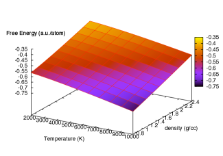
Figure 1: Free energy surface of hydrogen as a function of temperature and density.

In this paper we calculate the free energy of hydrogen as a function of temperature and density. We explore the range 2 000K $<$ T $<$ 10 000K and 0.7 g cm^-3 $<\rho<$ 2.4 g cm^-3. For $\rho$ $<$ 0.7 g cm^-3, molecular dissociation becomes the dominant feature in the EOS, requiring a more detailed study than the one performed here to reach a similar level of accuracy. Simulations of the molecular liquid are in progress.

The CEIMC calculations were performed with 54 hydrogen atoms using RQMC. The time step and projection length used in RQMC were chosen to reach a convergence of the energy of 0.2-0.3 mHa/atom; see appendix C for details. We used TABC with a grid of 64 twists (96 for $r_{s}\leq 1.10$), which together with the use of recently developed finite-size correction schemes for QMC energies, allows a significant reduction of size effects; see appendix B for details and discussion.

We performed a 36 CEIMC simulations (not including those related to the coupling constant integration), the results are reported in Table III of appendix A. Our simulations were first equilibrated using effective pair potentials built from reflected Yukawa functions, which were chosen such they reproduced the radial distribution functions of the QMC systems. We then performed 2000-3000 equilibration steps with CEIMC. Statistics were gathered in the following 5000-15000 steps, the number depending on temperature and density.

The protons are treated as classical particles in the results presented in Table III and in the free energy calculations discussed below. Quantum effects of the protons could be important at low temperatures at the densities considered in this work. In order to assess their effect on the thermodynamic properties, we performed Path Integral Monte Carlo (PIMC) calculations for the protons on the potential energy surface defined by the zero temperature RQMC method. This is an extension of CEIMC to path integral calculations Pierleoni06 . The resulting corrections to the energy and pressure are given in Table I, at T= 2000K for 3 densities. At this temperature, which is the lowest temperature studied in this work, the corrections to the pressure are below 1$\%$.

$r_{s}$	$\Delta E$ (mHa)	$\Delta P$ (GPa)
1.05	4.0 (7)	7 (3)
1.10	3.8 (3)	9 (1)
1.25	2.8 (5)	5 (1)

Table 1: Corrections to the energy and pressure of hydrogen from quantum effects of the protons, from PIMC simulations with CEIMC, at a temperature of 2000 K: $\Delta E=(E-E_{classical})/N$ and $\Delta P=P-P_{classical}$. Errors in parentheses.

III.1 Free Energy Integration

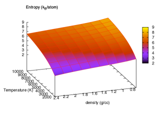
Figure 2: The entropy per atom as a function of temperature and density.

We used Coupling Constant Integration (CCI) Kirkwood35 to calculate the free energy of hydrogen at a reference point chosen as T=6000K and $r_{s}=1.25$. In CCI a $\lambda$-dependent potential energy, $V(\lambda)$, is a linear combination of two different potentials: $V(\lambda)=V_{0}+\lambda(V_{1}-V_{0})$. The difference in free energy between systems $0$ and $1$ is then:

$$F_{1}-F_{0}=\int_{0}^{1}d\lambda\left<(V_{1}-V_{0})\right>_{V(\lambda)}.$$ (7)

We chose the reference potential to be a reflected Yukawa pair potential:

$$V_{0}(r)=\begin{cases}\frac{e^{-br}}{r}+\frac{e^{-b(L-r)}}{(L-r)}-4\frac{e^{-bL/2}}{L}&r\leq L/2,\\ 0&r>L/2,\end{cases}$$ (8)

where b=2.5 a.u. and L is the length of the simulation cell. The reflection makes the function and its first derivative continuous at the cut-off, $r=L/2$. We first used CCI to calculate the free energy difference between the Yukawa potential and a system of non-interacting particles. We performed a second CCI with CEIMC to calculate the free energy difference between the Yukawa model and the QMC system. We obtained a value of -0.5737(1) Ha/atom for the free energy and 1.98(1)$\ast 10^{-5}$ (Ha/K) for the entropy at the reference point.

III.2 Fits to EOS

The free energy as a function of temperature and density was obtained by using the functional form:

$$F(T,\rho)=\sum_{i=1}^{4}\sum_{k=1}^{5}c_{ik}\ g_{i}(T)\ g_{k}(\rho),$$ (9)

where $g_{i}(x)=\{1,x,x^{2},x\ln{x},x^{2}\ln{x}\}$. We do a least squares fit between the analytical function and the CEIMC data using derivatives of this expansion:

$$P(T,\rho) = \frac{\rho^{2}}{m_{h}}\left(\frac{\partial{F}}{\partial{\rho}}\right)_{T}$$ (10)

$$E(T,\rho) = -T^{2}\left[\frac{\partial}{\partial{T}}\left(\frac{F}{T}\right)\right]_{\rho}$$ (11)

The free energy fit reproduces the energies and pressures obtained from the CEIMC simulations to within 0.5$\%$ and 1.5$\%$ respectively, although the average error is much smaller than this. Figures 1 and 2 show plots of the free energy and entropy in the region of the phase diagram studied. The coefficients of the expansion are given in Table II.

k	$c_{1k}$	$c_{2k}$	$c_{3k}$	$c_{4k}$
1	-0.529586	-2.085591$\cdot 10^{-4}$	-3.365628$\cdot 10^{-9}$	2.294411$\cdot 10^{-5}$
2	2.227221$\cdot 10^{-6}$	-1.452601$\cdot 10^{-4}$	-2.488880$\cdot 10^{-9}$	1.894880$\cdot 10^{-5}$
3	-6.266619$\cdot 10^{-5}$	4.210279$\cdot 10^{-4}$	6.174066$\cdot 10^{-9}$	-5.144879$\cdot 10^{-5}$
4	9.977346$\cdot 10^{-2}$	-6.220508$\cdot 10^{-4}$	-8.564851$\cdot 10^{-9}$	7.499558$\cdot 10^{-5}$
5	-1.437627$\cdot 10^{-2}$	-9.867541$\cdot 10^{-5}$	-1.598083$\cdot 10^{-9}$	1.225739$\cdot 10^{-5}$

Table 2: Coefficients of the expansion of the free energy; energy in Hartree/atom, temperature in K and density in g $cm^{-3}$

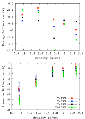
Figure 3: Comparison of EOS data with DFT-based BOMD simulations.

IV Comparison with other methods

Figure 3 shows a comparison of the pressure and energy between CEIMC simulations and DFT based Born-Oppenheimer Molecular Dynamics (BOMD) simulations. The BOMD simulations were performed in the NVT-ensemble (with a weakly coupled Berendsen thermostat) using the Qbox code . We used the Perdew-Burke-Ernzerhof (PBE) exchange-correlation functional and a Hamman type Hamman89 local pseudopotential with a core radius of $r_{c}$ = 0.3 $a.u.$ to represent hydrogen. The simulations were performed with 250 hydrogen atoms using a plane-wave cutoff of 90 Ry (115 Ry for rs $\geq$ 1.10)with periodic boundary conditions ($\Gamma$ point). Corrections to the EOS were added to extrapolate results to infinite cutoff and to account for the Brillouin zone integration. To do this we studied 15-20 statistically independent static configurations at each density by using a 4x4x4 grid of k-points with a plane-wave cutoff of at least 300 Ry. See ref. Morales09 for additional details of the DFT simulations.

There is a good agreement between the two methods, especially at higher densities where the difference in pressure is within error bars. At lower densities, the pressure difference increases reaching an average of approximately 5$\%$ close to the dissociation regime. There is less reason to expect exact agreement of the energies calculated since the DFT calculations use pseudopotentials as well as approximate exchange-correlation functionals which can modify the zero of energy. However, the temperature and density dependence is well reproduced with an almost uniform energy difference of 0.8$\%$ on the entire phase diagram. Figure 4 shows a comparison of the proton-proton distribution function for several thermodynamic conditions. The agreement between the two methods is again remarkable. The structure of the liquid is reproduced by the DFT simulations quite accurately, even the short range correlation peak that develops at the lower temperatures and higher densities. Figure 5 shows a comparison of the entropy as a function of density along several isotherms. We can see that for densities beyond $\rho=1.4g/cm^{3}$, the entropies obtained with the two methods are undistinguishable. In general, we obtain very good agreement between the two methods for pressures beyond 600 GPa. At lower pressures, the agreement is not perfect, but still very good, with BOMD predicting a slightly higher entropy than CEIMC. We are currently expanding our calculations to lower density to provide an additional benchmark of the DFT method close to the molecular dissociation region.

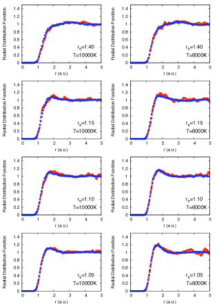
Figure 4: Comparison of radial distribution functions between BOMD (blue) and CEIMC (red).

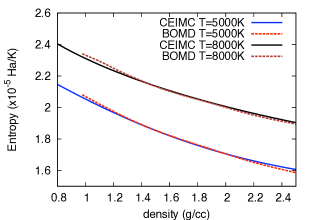
Figure 5: The entropy/atom at 5000K and 8000K as determined with BOMD and CEIMC.

Figure 6 shows a comparison of the pressure as a function of density obtained with CEIMC and BOMC and the SCVH equation of state at T=6000 K. At pressures well below the dissociation regime, SCVH produces very good results, but at higher densities the model can not capture all the features which result from strong atomic coupling; it predicts a qualitatively different behavior with higher pressures at lower densities.

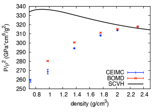
Figure 6: Comparison of pressure (divided by $\rho^{2}$) as a function of density computed with SCVH, BOMD and CEIMC at T=6000 K.

V Conclusions

In summary, we performed a comprehensive study of the free energy and the equation of state of warm dense liquid hydrogen in its atomic phase using energies computed with quantum Monte Carlo methods. We provide a fit to the free energy which can be used as input to models of Jovian planets or in the formulation of more accurate chemical models. Given the current status of DFT and its possible limitations at these conditions, it is crucial to benchmark its predictions against more accurate methods. We provide such a critical test. Our results indicate that DFT-based BOMD simulations provide a very good description of both thermodynamic and structural properties of hydrogen for the studied conditions. The equation of state of SCVH, used in the study of planetary interiors for more than a decade, is shown to produce inaccurate results in the atomic regime. This suggests that planetary models should be reinvestigated with a more accurate equations of state, such as the one presented in this work.

Appendix A Equation of State Table

Table III gives the energy per atom and pressure as calculated by CEIMC on a grid in temperature and density. Finite size corrections (see next section) are included in the reported results, as well as corrections to the pressure from non-zero time step and finite projection time in RQMC. The latter corrections are negligible in the case of total energies.

T (K)	rs	Energy (Ha)	Pressure(GPa)
2000	1.05	-0.3846 (3)	1576 (2)
3000	1.05	-0.3777 (2)	1607 (1)
4000	1.05	-0.3707 (5)	1640 (3)
6000	1.05	-0.3569 (4)	1701 (2)
8000	1.05	-0.3458 (4)	1753 (2)
10000	1.05	-0.3316 (8)	1814 (4)
2000	1.10	-0.4170 (2)	1157 (2)
3000	1.10	-0.4097 (2)	1190 (1)
4000	1.10	-0.4026 (3)	1219 (1)
6000	1.10	-0.3898 (4)	1270 (2)
8000	1.10	-0.3777 (5)	1315 (2)
10000	1.10	-0.3660 (4)	1362 (2)
2000	1.15	-0.4419 (2)	861 (1)
3000	1.15	-0.4356 (3)	883 (2)
4000	1.15	-0.4285 (7)	911 (3)
6000	1.15	-0.4151 (6)	956 (3)
8000	1.15	-0.4018 (9)	1003 (3)
10000	1.15	-0.3891 (8)	1048 (2)
2000	1.25	-0.4790 (2)	485 (1)
3000	1.25	-0.4721 (2)	504 (1)
4000	1.25	-0.4673 (4)	517 (2)
6000	1.25	-0.4549 (6)	556 (1)
8000	1.25	-0.4419 (7)	590 (3)
10000	1.25	-0.4324 (7)	619 (2)
2000	1.40	-0.5117 (4)	214 (1)
3000	1.40	-0.5057 (2)	222 (1)
4000	1.40	-0.4993 (5)	234 (1)
6000	1.40	-0.4869 (5)	257 (3)
8000	1.40	-0.4767 (5)	277 (1)
10000	1.40	-0.4674 (4)	297 (1)
2000	1.55	-0.5330 (2)	111 (1)
3000	1.55	-0.5230 (2)	105 (1)
4000	1.55	-0.5157 (3)	117 (1)
6000	1.55	-0.5027 (4)	134 (1)
8000	1.55	-0.4938 (2)	143 (1)
10000	1.55	-0.4831 (6)	163 (2)

Table 3: Energy/atom and pressure as calculated with CEIMC. Statistical errors are given in parentheses.

Appendix B Finite Size Effects

Due to the high computational demands of QMC, our simulations are restricted to systems with 128 atoms or fewer. Many techniques have been developed in order to obtain useful results with finite systems. In this work we use TABC (the generalization of Brillouin zone integration to many-body quantum systems) to eliminate shell effects in the kinetic energy of metallic systems. Twisted boundary conditions when an electron wraps around the simulation box are defined by:

$$\Psi_{\theta}(...,\vec{r_{j}}+\vec{L},...)=e^{i\theta}\Psi_{\theta}(...,\vec{r_{j}},...).$$ (12)

Observables are then averaged over the all twist vectors, similar to one-body theories:

$$<\hat{A}>=\int_{-\pi}^{\pi}\frac{d\vec{\theta}}{(2\pi)^{3}}<\Psi_{\theta}|\hat{A}|\Psi_{\theta}>.$$ (13)

This has been shown to restore the $1/N$ dependence of the energy in QMC calculations, absent when PBC are used.

As first shown by Chiesa et.al. Chiesa06 , most of the remaining finite size errors in the potential and kinetic energies of QMC simulations come from discretization errors induced by the use of PBC. To see this, notice that we can write the potential energy of a system of N electrons as:

$$<\hat{V}>=\frac{1}{2\Omega}\sum_{\vec{k}\neq 0}v(\vec{k})[S_{N}(\vec{k})-2N],$$ (14)

where $\Omega$ is the volume of the supercell, $v(\vec{k})$ is the Fourier transform of the Coulomb potential, $S_{N}(\vec{k})$ = $<\rho(\vec{k})\rho(-\vec{k})>$ is the structure factor, $\rho(\vec{k})=\sum_{i}z_{i}e^{i\vec{k}\cdot\vec{r_{i}}}$ and $\vec{k}$ is the set of lattice vectors in reciprocal space of the supercell. As we approach the thermodynamic limit $N\rightarrow\infty$, the structure factor converges ($S_{N}(\vec{k})\rightarrow S_{\infty}(\vec{k})$) and the sum becomes an integral: $\frac{1}{V}\sum_{\vec{k}\neq 0}\rightarrow\int\frac{d\vec{k}}{(2\pi)^{3}}$. If we assume that the structure factor is essentially converged for some finite number of atoms, then most of the finite size error in the potential energy comes from the omission of the $\vec{k}=0$ term in the sum. This can be estimated using the Poisson summation formula:

$$\int\frac{d\vec{k}}{(2\pi)^{3}}\hat{\eta}(\vec{k})-\sum_{\vec{k}\neq 0}\hat{\eta}(\vec{k})=\eta(0)-\sum_{\vec{L}}\eta(\vec{L}).$$ (15)

We know from the RPA, exact in the limit of $\vec{k}\rightarrow 0$, that $S(\vec{k})\approx k^{2}$ as $k\rightarrow 0$. The leading order correction to the potential energy is:

$$\delta V=\frac{3}{2Nr_{s}^{3}}\lim_{\vec{k}\rightarrow 0}\frac{S(\vec{k})}{k^{2}}.$$ (16)

By estimating the structure factor for small k during our simulation and extrapolating its behavior to k=0, we obtain the desired corrections. In the case of the kinetic energy, following a similar argument we obtain for the correction to second order Chiesa06 ; Drummond08 :

$$\delta K = \int\frac{d\vec{k}}{(2\pi)^{3}}u(\vec{k})k^{2}-\sum_{\vec{k}\neq 0}u(\vec{k})k^{2}$$ (17)

$$= \frac{\sqrt{3}}{4Nr_{s}^{3/2}}-\frac{5.264}{2\pi r_{s}^{2}(2N)^{4/3}},$$

where $u(\vec{k})$ is the electron-electron Jastrow; we used its RPA form.

To check the finite-size corrections for dense hydrogen, we performed simulations with 32, 54 and 108 atoms at $r_{s}$=1.85 and $r_{s}$=1.25. We used TABC with Variational Monte Carlo energies with 108 twists for the 32 atom system and 32 twists for the 54 and 108 atoms. Figure 7 shows a comparison of the radial distribution functions between the systems with different number of atoms, for the two densities studied. As can be seen, the agreement between the 3 simulations is very good, with no noticeable difference between the systems with 54 and 108 atoms. Using the fact that TABC restores the 1/N dependence of the properties, we can compare the results of the size correction formulas with a 1/N extrapolation. Table IV shows a comparison of finite size corrections taking the system with 54 atoms as the reference. As can be seen, the correction for the lower density system agrees very well with the extrapolated value. In the case of the higher density system, the agreement is less good but still acceptable. We attribute the disagreement at higher densities to the differences in TABC used for the systems with different sizes.

$r_{s}$	Energy (mHa)		Pressure (GPa)
	$\Delta E_{N}$	$\Delta E_{S}$	$\Delta P_{N}$	$\Delta P_{S}$
1.25	7.7	10.0	10.8	17.6
1.85	5.4	5.5	3.3	3.1

Table 4: Comparison of finite-size corrections between a size extrapolation ($\Delta E_{N}$,$\Delta P_{N}$) and formulas B5 and B6 ($\Delta E_{S}$,$\Delta P_{S}$).

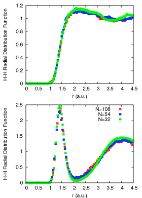
Figure 7: Comparison of proton-proton radial distribution functions between systems with different number of electrons. In the upper panel, the temperature is 4000K and r_s=1.25. In the lower panel, the temperature is 3000K and r_s=1.85. Electronic energies in CEIMC were calculated using Variational Monte Carlo.

Appendix C Details of RQMC calculations

As mentioned in the text, the parameters of the RQMC calculations were varied with density to obtain uniform accuracy over the whole phase diagram. Table V shows the time steps and projection times used in the simulations for the different densities studied. As is well known, total energies converge faster as a function of imaginary time because their convergence error is second order with respect to the trial wavefunction. The kinetic and potential energies, and hence the pressure, are only first order, which means that longer projection times are needed to obtain converged results. During the course of the simulations, we only require accurate energies, so a smaller projection time is used; one that is insufficient for accurate pressures. In order to obtain converged results for the pressure, we calculated a correction for the finite projection time and non-zero time step by studying approximately a dozen protonic configurations at each density. The corrections were found to be independent of the precise proton configuration but density dependent. The corrections to the total energy are negligible within errors.

$r_{s}$	projection time $(a.u.)^{-1}$	time step (a.u.)
1.05	0.456	0.008
1.10	0.504	0.008
1.15	0.550	0.01
1.25	0.660	0.012
1.40	0.732	0.012
1.55	0.975	0.015

Table 5: Projection time and time step used in the RQMC calculations.

- (1) Guillot T., Annu Rev Earth Planet Sci 33, 493 (2005).
- (2) Loubeyre P, Occelli F, LeToullec R., Nature (London) 416, 613 (2002).
- (3) Hicks D.G., et.al., Phys. Rev. B 79, 014112 (2009).
- (4) Nellis WJ, Rep. Prog. Phys. 69, 1479 (2006).
- (5) Saumon D, Chabrier G, Van Horn HM, Astrophys J Suppl S 99, 713 (1995).
- (6) Sandia Report
- (7) R Redmer et al, J. Phys. A: Math. Gen. 39, 4479 (2006).
- (8) Militzer B, Ceperley DM, Phys. Rev. Lett. 85, 1890 (2000).
- (9) Lenosky TJ, Bickham SR, Kress JD, Collins LA, Phys Rev B 61, 1 (2000), Lenosky LA et al, Phys Rev B 63, 184110 (2001).
- (10) Desjarlais MP, Phys Rev B 68, 064204 (2003).
- (11) Scandolo S, Proc Natl Acad Sci USA 100, 3051 (2003).
- (12) Bonev SA, Militzer B, Galli G, Phys. Rev. B 69, 014101 (2004).
- (13) Bonev SA, Schwegler E, Ogitsu, Galli G, Nature 431, 669 (2004).
- (14) Vorberger J, Tamblyn I, Militzer B, Bonev SA, Phys Rev B 75, 024206 (2007).
- (15) Holst B, Redmer R, Desjarlais M,Phys. Rev. B 77, 184201 (2008).
- (16) Militzer B, et al, Astrophys J Lett 688 (2008) L45.
- (17) Umrigar CJ, et al, Phys. Rev. Lett. 98, 110201 (2007).
- (18) Rios PL, et al, Phys Rev E 74, 066701 (2006).
- (19) Grossman J, et al, Phys Rev Lett 86, 472 (2000).
- (20) Dewing M, Ceperley DM, Pierleoni C, Lecture Notes in Physics 605, 473-499 (2002).
- (21) Pierleoni C, Ceperley DM, Lecture Notes in Physics 714, 641-683 (2006).
- (22) Ceperley DM, Dewing M, J. Chem. Phys. 110, 9812-9820 (1999).
- (23) Lin C, Zong FH, Ceperley DM, Phys Rev E 64, 016702 (2001).
- (24) Chiesa S, Ceperley DM, Martin RM, Holzmann M, Phys. Rev. Letts. 97, 076404 (2006).
- (25) Drummond N, Needs RJ, Sorouri A, Foulkes M, Phys Rev B 78, 125106 (2008).
- (26) Pierleoni C, Delaney KT, Morales MA, Ceperley DM, Holzmann M, Comput Phys Commun 179 89 (2008).
- (27) Pierleoni C, Ceperley DM, Holzmann M, Phys Rev Lett 93, 146402 (2004).
- (28) Baroni S, Moroni S, Phys. Rev. Lett. 82, 4745 - 4748 (1999).
- (29) Pierleoni C, Ceperley DM, ChemPhysChem 6, 1 (2005).
- (30) Kwon Y, Ceperley DM, Martin RM, Phys. Rev. B 48, 12037 (1993).
- (31) Perdew J, Zunger A, Phys. Rev. B 23, 5048 - 5079 (1981).
- (32) Ceperley DM, Alder BJ, Phys. Rev. Lett. 45, 566 (1980).
- (33) Holzmann M, Ceperley DM, Pierleoni C, Esler K, Phys. Rev. E 68, 046707:1-15 (2003).
- (34) Kirkwood JG, J. Chem. Phys. 3, 315 (1935).
- (35) Hamman DR, Phys. Rev. B 40, 2980-2987 (1989).
- (36) Morales MA et al, PNAS 106, 1324-1329 (2009).