Structure and decay of rotating homogeneous turbulence

Abstract

Navier-Stokes turbulence subject to solid-body rotation is studied by high-resolution direct numerical simulations (DNS) of freely decaying and stationary flows. Setups characterized by different Rossby numbers are considered. In agreement with experimental results strong rotation is found to lead to anisotropy of the direct nonlinear energy flux, which is attenuated primarily in the direction of the rotation axis. In decaying turbulence the evolution of kinetic energy follows an approximate power law with a distinct dependence of the decay exponent on the rotation frequency. A simple phenomenological relation between exponent and rotation rate reproduces this observation. Stationary turbulence driven by large-scale forcing exhibits $k_{\perp}^{-2}$-scaling in the rotation-dominated inertial range of the one-dimensional energy spectrum taken perpendicularly to the rotation axis. The self-similar scaling is shown to be the cumulative result of individual spectral contributions which, for low rotation rate, display $k_{\perp}^{-3}$-scaling near the $k_{\parallel}=0$ plane. A phenomenology which incorporates the modification of the energy cascade by rotation is proposed. In the observed regime the nonlinear turbulent interactions are strongly influenced by rotation but not suppressed. Longitudinal two-point velocity structure functions taken perpendicularly to the axis of rotation indicate weak intermittency of the $k_{\parallel}=0$ (2D) component of the flow while the intermittent scaling of $k_{\parallel}\neq 0$ (3D) fluctuations is well captured by a modified She-Lévêque intermittency model which yields the expression $\zeta_{p}=p/6+2(1-(2/3)^{p/2})$ for the structure function scaling exponents.

1 Introduction

Hydrodynamic turbulence subject to rotation is an ubiquitous problem in fluid mechanics. The understanding of its detailed properties is crucial for engineering problems such as the design of turbomachinery and for the understanding of atmospheric and oceanic flows influenced by the earth’s rotation. These applications have motivated an extensive research on the macroscopic and spectral properties of rotating turbulence though a comprehensive and fully consistent physical picture is still missing.

Early experiments show the tendency of rotating turbulence to asymptotically two-dimensionalize in planes perpendicular to the rotation axis $\boldsymbol{\Omega}$, where $\Omega=|\boldsymbol{\Omega}|$ is the rotation frequency. Signatures of this behaviour are, e.g., an increased ratio of velocity correlation lengths along and perpendicular to the axis of rotation, (see, for example, Ibbetson & Tritton, 1975), visible elongation of spatial structures along $\boldsymbol{\Omega}$, (e.g. in Hopfinger et al., 1982), or anisotropy of characteristic length- and time-scales (e.g. Wigeland, 1978; Jacquin et al., 1990). In addition, slower decay of kinetic energy is found in the works of Wigeland (1978) and Jacquin et al. (1990) as compared to non-rotating turbulence. More recently, the experiments of Morize & Moisy (2006) show the significant influence of confinement on the decay of rotating turbulence. Baroud et al. (2002, 2003) consider two-point increment statistics up to order $p=10$ yielding inertial-range scaling exponents $\zeta_{p}=p/2$. The work of Morize et al. (2005) focuses on the energy spectrum $E(k)$ which exhibits a Rossby number dependent scaling exponent continuously ranging between -5/3 (slow rotation) and about -2.3 (fast rotation). Both experiments feature turbulent flows with energy injection at intermediate scales and thus allow an inverse cascade of kinetic energy to develop in the quasi-two-dimensional flow expected for strong rotation.

The first direct numerical simulations of rotating turbulence conducted by Bardina et al. (1985), Mansour et al. (1992) and Hossain (1994) also suggest reduction of the energy flux and two-dimensionalization. They suffer, however, from small spatial resolution and correspondingly low Reynolds numbers and do not yield conclusive results on the spectral properties of the flow. Simulations at higher Reynolds number by Godeferd & Lollini (1999) and Morinishi et al. (2001) provide more evidence for the experimentally observed behaviour of the correlation lengths and the decay properties of the kinetic turbulent energy, respectively. For the case of driven turbulence Yeung & Zhou (1998) find $k^{-2}$-scaling of the energy spectrum in a setup with large scale forcing. On the contrary, the simulations of Smith & Waleffe (1999), Chen et al. (2005) and Mininni et al. (2009) explore systems with forcing at intermediate scales. All three works identify a quasi-two-dimensional state in the case of strong rotation accompanied by an inverse energy cascade for wavenumbers $k<k_{\mathrm{forcing}}$. In this wavenumber range Smith & Waleffe (1999) report to find $k^{-3}$-scaling of the energy spectrum while a $k^{-2}$-behaviour for $k>k_{\mathrm{forcing}}$ is observed by Smith & Waleffe (1999) and Mininni et al. (2009).

Large-Eddy simulations like those of Squires et al. (1993), Bartello et al. (1994) and Yang & Domaradzki (2004) are a useful tool to study the effects of rotation on characteristic properties of rotating turbulence such as the slowing down of energy decay, the large-scale structure of the flow and its tendency to become two-dimensional. The approach allows to attain Reynolds numbers beyond the reach of DNS. However, the results of LES crucially depend on the applied subgrid model which requires careful adjustments and gauging by comparison with high-resolution DNS or experimental measurements. For the detailed numerical investigation of small-scale properties of turbulence like anisotropic inertial-range scaling of the energy spectrum and higher-order structure functions, therefore, the DNS approach is chosen in this work.

Different theoretical approaches exist with regard to rotating turbulence. Shell-models, which are strongly simplified representations of nonlinear turbulent dynamics, allow for the straightforward inclusion of rotation effects, e.g. via modes governed by a time-correlated stochastic process as in Hattori et al. (2004). The simplicity of those models, however, restricts their predictive capabilities to a continuous change of spectral scaling between Kolmogorov $k^{-5/3}$-scaling (slow rotation) and $k^{-2}$-behaviour for fast rotation. Zhou (1995) and Mahalov & Zhou (1996) recover $k^{-2}$-scaling of the energy spectrum in the context of quasi-normal closure theory using dimensional arguments first employed by Kraichnan (1965). Canuto & Dubovikov (1997) arrive at similar results via a formal treatment of the spectral energy flux using helical-mode decomposition. The former work is based on the assumption that $\tau_{\Omega}=\Omega^{-1}$ is the dominant time scale of nonlinear relaxation while the latter study is analytically showing the same covering cascade dynamics for rotation rates up to $\tau_{\Omega}\simeq\tau_{\mathrm{NL}}\sim\ell/v_{\ell}$. Here, $\tau_{\mathrm{NL}}$ is the nonlinear eddy-turnover or relaxation time defined with the RMS velocity $v_{\ell}$ at scale $\ell$ (see below). On the contrary, weak turbulence theory (see, e.g., Cambon et al., 2004; Galtier, 2003; Bellet et al., 2006) yields different anisotropic scaling relations but is only strictly applicable in the asymptotic limit $\tau_{\Omega}\ll\tau_{\mathrm{NL}}$.

This article is motivated by the lack of a simple dynamical picture of spectral energy transfer which could also help to improve the understanding of turbulent energy decay. The proposed phenomenology is backed-up by high-resolution direct numerical simulations of incompressible rotating homogeneous turbulence in free decay and of rotating turbulence subject to large-scale driving. The kinetic energy is found to exhibit approximate power-law decay with an exponent that decreases with increasing rotation frequency. This behaviour is in agreement with the observed attenuation of nonlinear spectral transfer under the influence of rotation and is captured by a simple model based on the cascade phenomenology. In the case of forced turbulence, analysis of one-dimensional spectral data indicates anisotropic energy flux mainly perpendicular to $\boldsymbol{\Omega}$. Inertial-range scaling of the perpendicular energy spectrum $\sim k_{\perp}^{-2}$ is observed and reproduced by the dynamical cascade phenomenology. While the parallel spectrum does not show clear scaling, the perpendicular spectra at fixed $k_{\parallel}$ display $k^{-3}$-scaling in the vicinity of $k_{\parallel}=0$ for low rotation rate. For growing $\Omega$, energy accumulates at $k_{\parallel}=0$ in agreement with the observed quasi-two-dimensionalization of the system. The intermittency measured via velocity structure functions perpendicular to $\boldsymbol{\Omega}$ is very weak for the 2D component of the flow ($k_{\parallel}=0$). In contrast, the intermittent scaling signature of the 3D component ($k_{\parallel}\neq 0$) is in agreement with a modified She-Lévêque model and exhibits a weak trend towards Gaussianity for high rotation rate. The remainder of this paper is organized in the following way: In section 2 we introduce the equations of rotating fluid flow and present the numerical methods that have been used. Sections 3 and 4 comprise the results on spectral and macroscopic properties of the flow and a summary is given in section 5.

2 Basic equations and numerical methods

Incompressible fluid flow subject to solid-body rotation is usually described in a frame of reference rotating about a fixed axis $\boldsymbol{\Omega}=\Omega\boldsymbol{\hat{e}}_{z}$ with frequency $\Omega$ using the dimensionless Navier-Stokes equations including the Coriolis force,

$$\partial_{t}\boldsymbol{v}+\boldsymbol{v}\cdot\nabla\boldsymbol{v} = -\nabla P+\mu\Delta\boldsymbol{v}+2\,{\Omega}\,\boldsymbol{v}\times\boldsymbol{\hat{e}}_{z},$$ (1)

$$\nabla\cdot\boldsymbol{v} = 0\,,$$ (2)

where the centrifugal force has been incorporated in the generalized pressure $P$, or the numerically more favourable vorticity formulation

$$\partial_{t}\boldsymbol{\omega} = \nabla\times(\boldsymbol{v}\times\boldsymbol{\omega}+2\,{\Omega}\,\boldsymbol{v}\times\boldsymbol{\hat{e}}_{z})+{\mu}\Delta\boldsymbol{\omega},$$ (3)

$$\nabla\cdot\boldsymbol{v} = 0\,$$ (4)

with the vorticity $\boldsymbol{\omega}=\nabla\times\boldsymbol{v}$ (see, e.g., Greenspan, 1968). The dimensionless kinematic viscosity ${\mu}$ and rotation rate ${\Omega}$ are both assumed to be constant.

Equations (3) and (4) are integrated numerically on a cubic box extending $2\pi$ in each dimension with triply periodic boundary conditions. The integration is performed in a pseudospectral Fourier representation by applying an explicit leapfrog scheme. The diffusive term is incorporated using an integrating factor technique (see, e.g., Meneguzzi & Pouquet, 1989). The time step which is required for numerical stability by the Courant-Friedrichs-Lewy criterion ensures the temporal resolution of all inertial-wave oscillations present in the system. The aliasing error introduced by the pseudospectral approach is reduced by spherical mode truncation. The quasi-stationary state of the driven systems is sustained by a forcing which freezes all modes with $k\leq k_{f}=2$. The applied resolution is $512^{3}$ collocation points for forced and $256^{3}$ for decaying turbulence.

The isotropic initial state of the forced simulations is a smooth vorticity field with random phases and an energy spectrum $E(k)\sim\exp\left(-k^{2}/k_{0}^{2}\right)$, $k_{0}=4$. This configuration is integrated forward in time without forcing until the maximum of enstrophy is reached. After this period of time, which corresponds to one large-eddy-turnover time (LET) and to three units of time in the notation of this paper, the energy spectrum is fully developed in its spectral extent and the forcing is switched on. The spectral distribution of energy evolves self-consistently towards a state with a low-order power-law at largest scales and a Kolmogorov-type inertial range. As soon as total energy $E=\int_{V}dVv^{2}/2$ and dissipation $\varepsilon={\mu}\int_{V}dV\omega^{2}$ are statistically stationary with $E\simeq 1$ (more precisely: $0.87$ for $\Omega=5$ and $1.3$ for $\Omega=50$) and $\varepsilon\simeq 0.05$, ${\Omega}$ is set to a finite value. For decaying turbulence simulations a similar random initial field is generated and left to evolve freely for one LET before rotation is switched on. After the onset of rotation a statistically stationary state of turbulence is maintained in driven simulations for 10 or 15 large-eddy turnover times depending on the rotation rate. Decaying runs extend over approximately 12 LETs. The dimensionless kinematic viscosity is constant in all simulations.

The characteristic length $L_{0}$ and velocity $V_{0}$, necessary for the calculation of the macroscopic Rossby number, $\mathsf{Ro}=V_{0}/(2\Omega L_{0})$, and Reynolds number, $\mathsf{Re}=L_{0}V_{0}/\mu$, can only be determined a posteriori in homogeneous turbulence. Therefore, both quantities are estimated in the dimensionless system using $E$, $\varepsilon$, and $\Omega$ as $L_{0}\sim E/({\Omega}\varepsilon)^{1/2}$ and $V_{0}\sim E^{1/2}$. Hence Rossby and Reynolds numbers given in this paper are defined as $\mathsf{Ro}=\sqrt{\varepsilon/(4{\Omega}E)}$ and $\mathsf{Re}=\sqrt{E^{3}/({\Omega}\varepsilon)}/{\mu}$, respectively. Specific parameters of the performed simulations are summarized in table 1.

simulation	grid	forcing	${\Omega}$	${\mu}$	$t_{\mathrm{Sim}}$	Ro	Re
I	$512^{3}$	yes	5	$4\times 10^{-4}$	45	$5.3\times 10^{-2}$	4000
II	$512^{3}$	yes	50	$4\times 10^{-4}$	30	$1.3\times 10^{-2}$	2300
III	$256^{3}$	no	0-5	$1\times 10^{-3}$	36	$\infty$ – $2\times 10^{-2}$	300–1100

Table 1: Parameters for the different simulation runs: rotation rate $\Omega$, viscosity $\mu$, total duration $t_{\mathrm{Sim}}$, Rossby number Ro, and Reynolds number Re

3 Structure of the flow

An immediate impression of the structure of rotating turbulence is provided by visualizations of the flow field given in figure 1. The system shows a distinct structuring along the rotation axis which is especially pronounced for simulation II and indicates a strong velocity correlation along this direction. The observed trend to a quasi-two-dimensional state with faster rotation is in agreement with previous experimental findings (see above). It is the consequence of a nonlinear analogue of the Taylor-Proudman theorem (see Mahalov & Zhou, 1996; Chen et al., 2005). For more mathematically oriented works on, e.g., the dynamics of two- ($k_{\parallel}=0$) and three-dimensional ($k_{\parallel}\neq 0$) flow components as well as the issues of their non-vanishing mutual interaction in the limit $\Omega\rightarrow\infty$ see Babin et al. (2000) and references therein.

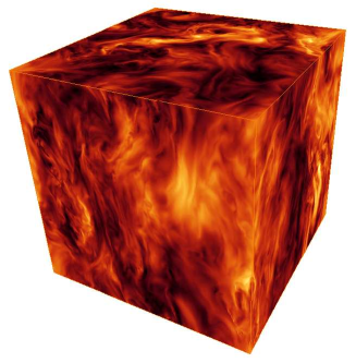
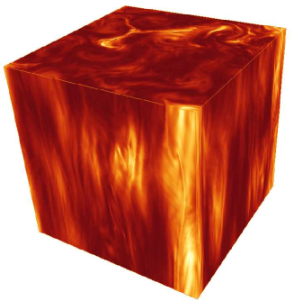
Figure 1: Visualization of the magnitude of the velocity field $|\boldsymbol{v}(\boldsymbol{r},t)|$ for simulations I (left) and II (right) in the statistically stationary regime of the flow. Brighter colours correspond to higher values of $|\boldsymbol{v}|$ and darker colours to lower values. The rotation axis points in the vertical direction. The pictures show the flow field of the whole $512^{3}$ simulation domain.

The clearest signature of the turbulent energy cascade is found in energy spectra and energy flux functions. Due to the above-mentioned anisotropy of the turbulence, one dimensional spectral quantities are considered in directions parallel and perpendicular to the rotation axis. The axis-parallel nonlinear energy flux over wavenumber $k_{\parallel}$ is given by $T_{k_{\parallel}}=\int_{0}^{k_{\parallel}}\mathrm{d}k_{\parallel}^{\prime}\int\mathrm{d}k^{\prime}\int\mathrm{d}k_{\perp}\left(i\boldsymbol{\omega}^{*}\cdot(\boldsymbol{k}\times\widetilde{\left[\boldsymbol{v}\times\boldsymbol{\omega}\right]}_{\boldsymbol{\scriptscriptstyle k}})+c.c.\right)/\boldsymbol{k}^{2}$, with $\widetilde{[\bullet]}$ denoting Fourier transformation, $\boldsymbol{k}_{\perp}\perp\boldsymbol{\Omega}$, $\boldsymbol{k_{\parallel}^{\prime}}\parallel\boldsymbol{\Omega}$, and $\boldsymbol{k^{\prime}}\perp\boldsymbol{k_{\perp}},\boldsymbol{k_{\parallel}^{\prime}}$. The axis-perpendicular flux function $T_{k_{\perp}}$ is defined analogously using the integration $\int_{0}^{k_{\perp}}\mathrm{d}k^{\prime}_{\perp}\int\mathrm{d}k^{\prime}\int\mathrm{d}k_{\parallel}$ with the $k_{\perp}$-component running along an arbitrary fixed direction in the axis-perpendicular plane. The fluxes are normalized with the total energy dissipation rate $\varepsilon=\mu\int\mathrm{d}V\omega^{2}$.

The parallel and perpendicular energy fluxes for $\Omega=0,5,50$ are negative at all wavenumbers indicating direct energy transfer towards small scales Müller & Thiele (2007). The two-dimensionalization visible in figure 1 is not in contradiction with the observed direct fluxes of energy which are a mere consequence of the large scale driving of the flow. The fluxes weaken with increasing $\Omega$, a trend that is much stronger in $T_{k_{\parallel}}$ than in $T_{k_{\perp}}$. The increasing anisotropy of the energy cascade with growing $\Omega$ reflects the nonlinear nature of the dynamical process that is at least partially responsible for the observed two-dimensionalization of the flow. The classical picture of energy transfer through eddy breakup relates a stronger eddy scrambling perpendicular to the rotation axis than in the parallel direction along which coherent structures remain comparatively intact.

The perpendicular energy spectra $E(k_{\bot})=\int dk_{\parallel}^{\prime}\int dk^{\prime}\left|v_{\boldsymbol{k}}\right|^{2}/2$ shown as solid lines in figure 2 display inertial range scaling for $4\lesssim k_{\perp}\lesssim 20$ (I) and $5\lesssim k_{\perp}\lesssim 16$ (II). The shortening of the scaling range with increasing rotation rate is due to an extension of the dissipation region towards smaller $k$ (see below). In simulation II a bump persists around $k_{f}$, where the forcing region descends into the freely evolving range of scales. It is a result of the simple forcing scheme and is tolerable at the chosen numerical resolution as it is not significantly perturbing the flow beyond $k\approx 5$.

In spite of the shortened inertial range in simulation II both cases clearly exhibit the scaling $E(k_{\bot})\sim k_{\bot}^{-2}$. These results agree with the direct numerical simulations of Yeung & Zhou (1998) and Smith & Waleffe (1999)(for $k>k_{f}$) as well as shell-model calculations (see Hattori et al., 2004). Recent experimental results on decaying turbulence subject to rotation (see Morize et al., 2005) yield an energy scaling exponent $\approx-2.5$ for the micro Rossby number of $\mathsf{Ro}_{\omega}=\langle\omega_{3}^{2}\rangle^{1/2}/(2\Omega)\simeq 0.08$ (corresponding to our case II) and an exponent of $\approx-1.7$ for $\mathsf{Ro}_{\omega}\simeq 0.7$ (corresponding to I). The experimental configuration with an initial excitation of the flow followed by decay under rotation is however not directly comparable to the simulations described here, which are characterized by a continuous large-scale forcing. We note in passing that these Rossby numbers place the present simulations in the “intermediate” Rossby number regime of Bourouiba & Bartello (2007). In the experiment of Baroud et al. (2002) the same scaling $\sim k^{-2}$ is observed although here forcing at the small scales produces an inverse energy cascade.

Several theoretical models arrive at the scaling shown in Fig. 2: In the context of quasi-normal closure theories Zhou (1995) and Mahalov & Zhou (1996) have conducted a dimensional analysis of the energy flux terms, assuming $\tau^{\ast}\sim\tau_{\Omega}\sim\Omega^{-1}$ for the relaxation timescale of nonlinear interactions $\tau^{\ast}$, whereas Canuto & Dubovikov (1997) have analyzed the energy flux formulated in helical mode decomposition, both arriving at the same scaling result. On the contrary, weak turbulence theory yields $E(k)\sim k^{-3}$ (see Cambon et al., 2004; Bellet et al., 2006) in the asymptotic quasi-normal Markovian approximation valid for $k_{\parallel}\neq 0$ and $E(k)\sim k^{-2}$ (see Galtier, 2003). The former result is regarded as the consequence of a strongly anisotropic spectral energy distribution with respect to $\boldsymbol{\Omega}$ while the latter explicitly assumes spectral isotropy in combination with a phenomenological nonlinear transfer time based on the wave-kinetic equation. Generally, however, wave turbulence theory predicts anisotropic scalings in the context of rotating turbulence.

Figure 2: Perpendicular two-dimensional spectra $E(k_{\parallel},k_{\bot})$ for $\Omega=5$ (left) and $\Omega=50$ (right) at fixed $k_{\parallel}$ and compensated with $k_{\bot}^{2}$. The spectrum for $k_{\parallel}=0$ (dotted) differs markedly from those for $k_{\parallel}=1-6$ (dashed lines from top down) and higher. Three-dimensional perpendicular spectra are obtained by $k_{\parallel}$-integration from $E(k_{\parallel},k_{\bot})$ (solid). The dash-dotted line indicates $k_{\perp}^{-3}$-scaling.

Figure 3: One-dimensional energy spectra parallel to the rotation axis compensated with $k_{\parallel}^{2}$ for $\Omega=5$ (solid), and $\Omega=50$ (dotted).

It is noteworthy that the axis-parallel spectra shown in figure 3 do not show clear scaling. This indicates that the perpendicular domain of wavenumbers provides the dominant contribution to the angle-averaged scaling $E(k)\sim k^{-2}$ found in some of the above-mentioned numerical and experimental studies.

The contributions to the perpendicular spectrum for fixed $k_{\parallel}$, shown in figure 2, exhibit for $\Omega=5$ $k^{-3}_{\perp}$-scaling in the vicinity of $k_{\parallel}=0$. Note that $E(k_{\perp})\sim\int dk_{\parallel}E(k_{\parallel},k_{\perp})\neq E(k_{\parallel}=const,k_{\perp})$. The scaling range, however, shrinks from the low $k$ side with growing $k_{\parallel}$. For $\Omega=50$ the spectral contributions for fixed $k_{\parallel}$ show no clear scaling. Evidently, the observed $k^{-2}_{\perp}$ power-law is due to spectral contributions from all wavenumbers $k_{\parallel}$. This observation is in contradiction to weak turbulence simulations reported in Bellet et al. (2006) which give $k^{-2}_{\perp}$-scaling in directions perpendicular to $\boldsymbol{\Omega}$ and suggest that $k^{-3}$-spectra are generated by spherical averaging. Furthermore and especially for $\Omega=50$, the energy is mainly concentrated around the plane $k_{\parallel}=0$ as expected from previous studies (see, e.g., Cambon & Jacquin, 1989; Cambon et al., 1997) and in agreement with the observed nonlinear two-dimensionalization.

The observed axis-perpendicular spectral scaling can be described by a simple phenomenology of rotating turbulence proposed in Müller & Thiele (2007) which tries to capture the effect of inertial oscillations on convective fluid motion. The phenomenology applies in the inertial-range under the additional constraint $k_{\Omega}>k>\min(k_{\mathrm{d}},k_{\mathrm{d}}^{\Omega})$, i.e. when nonlinear energy transfer is dominated by Coriolis force effects. This spectral interval is bounded by the rotation wavenumber $k_{\Omega}=(\Omega^{3}/\varepsilon)^{1/2}$ whose inverse, also called Rossby deformation radius, is analogous to the geophysical Ozmidov scale (see e.g. Ozmidov, 1992), the classical Kolmogorov dissipation wavenumber $k_{d}=(\varepsilon/\mu^{3})^{1/4}$, and its rotation-modified counterpart $k_{d}^{\Omega}=(\varepsilon/\Omega)^{1/2}/\mu$ (see, e.g., also Zeman, 1994; Canuto & Dubovikov, 1997).

For turbulent fluctuations $v_{\xi}$ perpendicular to $\boldsymbol{\Omega}$ on spatial scale $\xi\sim k_{\perp}^{-1}$ the influence of rotation on the inertial-range energy transfer in planes perpendicular to $\boldsymbol{\Omega}$ is phenomenologically described similarly to the Iroshnikov-Kraichnan picture of magnetohydrodynamic turbulence Iroshnikov (1964); Kraichnan (1965). Taking into account the random displacements that a fluid particle experiences during a nonlinear interaction of turbulent eddies under the influence of inertial oscillations leads to a prolonged energy transfer time $\tau_{\mathrm{tr}}\sim\tau_{\mathrm{NL}_{\perp}}^{2}/\tau_{\Omega}$ with $\tau_{\mathrm{NL}_{\perp}}\sim\xi/v_{\xi}$ as compared to the non-rotating case. This yields by standard dimensional arguments the non-intermittent scaling relation $v_{\xi}\sim(\Omega\varepsilon)^{1/4}\xi^{1/2}$ corresponding to the observed scaling of the energy spectrum $\sim k_{\perp}^{-2}$ (see also Zhou, 1995; Canuto & Dubovikov, 1997).

The numerical values of the characteristic wave numbers are for simulation (I): $k_{\Omega}\simeq 50$, $k_{d}^{\Omega}\simeq 250$, $k_{d}\simeq 167$, and for simulation (II): $k_{\Omega}\simeq 1581$, $k_{d}^{\Omega}\simeq 79$, $k_{d}\simeq 167$. It should be noted that, according to their definition, for increasing $\Omega$, $k_{\Omega}$ grows while $k_{d}^{\Omega}$ decreases. This is the reason for the smaller inertial range in system I and could also explain why in earlier works with lower resolution the scaling exponent of the energy spectrum for high rotation rates has been difficult to pin down.

The two-dimensionalization evident in figure 1, due to the large-scale driving, does not lead to an inverse energy cascade but still leaves some spectral traces that can be understood by the following ordering considerations: it is proposed that for fixed $\Omega$ the are three different regimes of rotating turbulence: a) turbulence with negligible rotation effects at $k\gg k_{\Omega}$, b) turbulence strongly dominated by the Coriolis force at $k\ll k_{\Omega}$ which is asymptotically described by weak-turbulence theory with the associated purely nonlinear two-dimensionalization via anisotropic nonlinear energy transfer, and c) rotating turbulence in the transient regime at $k\lesssim k_{\Omega}$ observed in the present simulations where quasi-two-dimensionalization occurs due to the “nonlinear Taylor-Proudman theorem” (see above). This effect entails an observable energetic separation of 2D ($k_{\parallel}=0$) and 3D ($k_{\parallel}\neq 0$) components of the velocity field which exhibit an energetically weaker coupling at high rotation rate (see, e.g., Bourouiba & Bartello, 2007, and references therein). It can, however, be shown rigorously (see e.g. Babin et al., 2000) that the dynamical coupling of 2D and 3D fluctuations remains finite for all values of $\Omega$. In regime a) turbulence is based on nonlinear eddy interaction, regime b) represents turbulence governed by (weak) wave interaction, while nonlinear dynamics underlying regime c) correspond to wave-modified eddy interaction. In regime c) the 2D fluctuations should exhibit dynamics different from the 3D fluctuations as indicated by the nonlinear Taylor-Proudman theorem. A possible scenario that would be in agreement with the observed scaling laws consists of a direct cascade of 3D energy as described by the proposed phenomenology in combination with an inverse cascade of 2D energy (towards wavenumbers smaller than the forcing range) or a direct enstrophy cascade (towards wavenumbers larger than the forcing range). In this picture the $k^{-3}$ inertial-range scaling of 2D energy could be interpreted as the signature of a direct 2D enstrophy cascade.

Regime c), in fact, describes a state of continuous transition from $\mathsf{Ro}\rightarrow\infty$ (negligible rotation) to $\mathsf{Ro}\rightarrow 0$ (weak inertial-wave-turbulence). This transitional state is applying to most realistic rotating systems. The dynamical phenomenology by Müller & Thiele (2007) could be a reasonable starting point for extending the theoretical description of rotating turbulence to include the growing influence of inertial waves on turbulence dynamics.

To obtain the scaling exponents $\zeta_{p}$ of the axis-perpendicular longitudinal velocity structure functions, $S_{p}=\langle|[\boldsymbol{v}(\boldsymbol{r})-\boldsymbol{v}(\boldsymbol{r}+\boldsymbol{\xi})]\cdot\boldsymbol{\xi}/\xi|^{p}\rangle\sim\xi^{\zeta_{p}}$ their extended self-similarity (ESS) first observed by Benzi et al. (1993) in the non-rotating case is exploited. By this heuristic but generally accepted procedure exponents up to order $p=8$ can be determined with sufficient precision in spite of the limited spatial resolution and overall duration of the simulations. The velocity field is resolved into a 2D component ($k_{\parallel}=0$) and 3D fluctuations ($k_{\parallel}\neq 0$) (see, e.g., Bourouiba & Bartello, 2007). The relative exponents $\zeta_{p}/\zeta_{2}$ obtained via ESS from the 3D velocity coincide with the $\zeta_{p}$ since the numerical results $E_{k_{\perp}}\sim k_{\perp}^{-2}\sim k_{\perp}^{-(\zeta_{2}+1)}$ yield $\zeta_{2}^{\mathrm{3D}}=1$. For the 2D component $\zeta_{2}^{\mathrm{2D}}=2$ is chosen consistently with the inertial-range scaling of the 2D energy spectrum $\sim k_{\perp}^{-3}$ (dotted line in figure 2).

The ESS-results shown in figure 4 and table 2 indicate a weakly intermittent structure of the 2D velocity component. The difference between exponents from non-rotating turbulence and those for $\Omega=50$ indicates that the reduction of intermittency for higher $\Omega$ is not a simple consequence of the removal of fluctuations with higher $k_{\parallel}$. The 3D fluctuations exhibit an intermittent signature that is up to order $p=7$ virtually independent of the rotation rate. The highest order scaling exponent is, however, suggesting slightly higher intermittency for $\Omega=5$ than for $\Omega=50$.

A comparison with two-point statistics obtained with the total turbulent velocity field including all $k_{\parallel}$ contributions Müller & Thiele (2007) reveals that the 2D-component of velocity tends to govern structure function scaling for $\Omega=50$. In contrast, the $\zeta_{p}$ taken with $\Omega=5$ are rather close to the values obtained with the $k_{\parallel}\neq 0$ velocity. The dominance of the 2D fluctuations in structure function scaling at high $\Omega$ is plausible because of the reduced activity of axis-perpendicular nonlinear interactions that is visible, e.g., in the corresponding energy flux Müller & Thiele (2007). The accompanying reduction of intermittency in the 2D flow component with higher rotation rate points towards stronger dynamical influence of inertial waves since weak wave-turbulence is generally non-intermittent. This effect is stronger in the 2D velocity than in the 3D component as the nonlinear energy flux is strongly depleted in the axis-parallel direction at high rotation rate compared to the axis-perpendicular flux (ibid.).

The 3D structure function scaling is well represented by an intermittency model based on the She-Lévêque (SL) ansatz She & Lévêque (1994). The SL-model is quite successful in describing intermittent scalings of two-point statistics in various non-rotating turbulent flows. It can be written in a general form exhibiting two parameters which can be determined by physical considerations Grauer et al. (1994); Politano & Pouquet (1995); Müller & Biskamp (2000): $\zeta_{p}=p/(3g)+C_{0}(1-(1-2/(3C_{0}))^{p/g})$. While $C_{0}$ stands for the co-dimension of the most singular dissipative structures, $g$ is connected to the basic nonintermittent scaling exponent, $v_{\ell}\sim\ell^{1/g}$. In the present three-dimensional simulations the most-singular structures are quasi-one-dimensional vortex filaments, i.e. $C_{0}=2$, while relation (10) yields g=2. This results in the intermittency model

$$\zeta_{p}=p/6+2(1-(2/3)^{p/2})$$ (5)

which agrees well with the numerical data as shown in figure 4 (see also table 2).

$p$	$\zeta_{p}^{\mathrm{2D,\Omega=5}}$	$\zeta_{p}^{\mathrm{2D,\Omega=50}}$	$\zeta_{p}^{\mathrm{nonintermitt}}$	$\zeta_{p}^{\mathrm{3D,\Omega=5}}$	$\zeta_{p}^{\mathrm{3D,\Omega=50}}$	$\zeta_{p}^{\mathrm{model}}$
1	$1.02\pm 0.03$	$1.0\pm 0.01$	1	$0.52\pm 0.003$	$0.52\pm 0.002$	$0.53$
2	$2$	$2$	2	$1$	$1$	$1$
3	$2.95\pm 0.06$	$2.99\pm 0.02$	3	$1.43\pm 0.006$	$1.43\pm 0.007$	$1.41$
4	$3.88\pm 0.1$	$3.97\pm 0.05$	4	$1.82\pm 0.02$	$1.80\pm 0.02$	$1.78$
5	$4.78\pm 0.2$	$4.94\pm 0.08$	5	$2.15\pm 0.03$	$2.13\pm 0.03$	$2.11$
6	$5.67\pm 0.3$	$5.91\pm 0.1$	6	$2.42\pm 0.05$	$2.42\pm 0.05$	$2.41$
7	$6.53\pm 0.4$	$6.86\pm 0.1$	7	$2.65\pm 0.07$	$2.68\pm 0.07$	$2.68$
8	$7.38\pm 0.5$	$7.81\pm 0.2$	8	$2.84\pm 0.1$	$2.91\pm 0.09$	$2.94$

Table 2: Structure function scaling exponents for 2D and 3D components of the velocity field with $\Omega=5$ and $\Omega=50$. The values are obtained by ESS assuming $\zeta_{2}^{\mathrm{3D}}=1$ and $\zeta_{2}^{\mathrm{2D}}=2$.

Figure 4: Axis-perpendicular structure function scaling exponents $\zeta_{p}$ of velocity fluctuations with $k_{\parallel}=0$ (left) and $k_{\parallel}\neq 0$ (right) up to order 8 for moderate, strong, and no rotation. Solid: $\Omega=5$, dotted: $\Omega=50$, dash-3-dot: $\Omega=0$, dashed: intermittency model (5), dash-dotted: non-intermittent scaling, $\zeta_{p}=p/2$ ($\Omega=5$) and $\zeta_{p}=p$ ($\Omega=50$).

To conclude the analysis of the structure of rotating turbulence we present probability density functions (PDFs) $P(\delta v_{\xi})$ of the axis-perpendicular longitudinal velocity increments $\delta v_{\xi}=[\boldsymbol{v}(\boldsymbol{r})-\boldsymbol{v}(\boldsymbol{r}+\boldsymbol{\xi})]\cdot\boldsymbol{\xi}/\xi$. Characteristic one-time PDFs for the 3D velocity field are shown in figure 5. For both rotation rates the PDFs shift from Gaussian form at large scales to functions with stretched exponential tails at small scales. This well-known behaviour indicates that both flows are intermittent in agreement with the structure function scaling. The tendency towards nonintermittent quasi-two-dimensional flow for increasing rotation rate is visible in the slight contraction of the normalized PDFs that is quantified by decreasing flatness, $S_{4}/(S_{2})^{2}$, taking on values of $9.4$ ($\Omega=5$) and of $7.8$ ($\Omega=50$) at small scales $\xi$. At large scales the flatness is, for both values of $\Omega$, close to $3$, a value characteristic for a Gaussian distribution. The skewness $S_{3}/S_{2}^{3/2}$ is also consistent with Gaussian statistics at large scales where it is ranging around zero. For $\Omega=50$ this behaviour is observed at all scales. For $\Omega=5$ the skewness drops to a level close to $-0.5$ at the small-scale end, a value known from non-rotating flow. Time-averaged flatness and skewness of the 3D velocity component are shown in figure 7. These findings suggest the existence of a self-similar limiting case for very high rotation rates (cf. Baroud et al., 2002).

Exemplary one-time PDFs for the 2D component of the velocity field are shown in figure 6, the associated time-averaged skewness and flatness functions are displayed in figure 8. In agreement with the weakly intermittent scaling of the corresponding structure functions, the PDFs at all spatial scales are close to Gaussian with the flatness increasing for growing $\Omega$ from $2.5$ ($\Omega=5)$ to $3.1$ ($\Omega=50$) at large scales and decreasing from $3.5$ ($\Omega=5$) to $3.2$ ($\Omega=50$) at small scales. With increasing rotation rate the skewness also changes from $-0.1$ (small scales) and about $0$ (large scales) for $\Omega=5$ to positive values close to $0$ at all scales for $\Omega=50$.

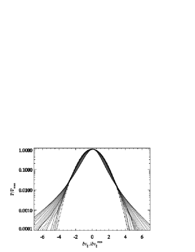
Figure 5: PDFs of 3D velocity differences ($k_{\parallel}\neq 0$) taken at different spatial distances (increasing from left to center in each plot) for $\Omega=5$ (left) and $\Omega=50$ (right). The width is rescaled by the velocity variance, and all curves are shifted to a common maximum at 1 to allow for simpler comparison with the shape of a Gaussian (dash-dotted curve).

Figure 6: PDFs of 2D velocity differences ($k_{\parallel}=0$) taken at different spatial distances for $\Omega=5$ (left) and $\Omega=50$ (right). The width is rescaled and all curves are shifted as in figure 5. The dash-dotted curve represents a Gaussian.

Figure 7: Time-averaged flatness $S_{4}(\xi)/(S_{2}(\xi))^{2}$ (left) and skewness $S_{3}(\xi)/(S_{2}(\xi))^{3/2}$ (right) of the PDFs corresponding to the 3D velocity fluctuations (figure 5) for for $\Omega=5$ (solid line), $\Omega=50$ (dashed line), and $\Omega=0$ (dash-3-dotted line). The dash-dotted lines display the respective values for a Gaussian.

Figure 8: Time-averaged flatness $S_{4}(\xi)/(S_{2}(\xi))^{2}$ (left) and skewness $S_{3}(\xi)/(S_{2}(\xi))^{3/2}$ (right) of the PDFs corresponding to the 2D velocity fluctuations (figure 6) for for $\Omega=5$ (solid line), $\Omega=50$ (dashed line), and $\Omega=0$ (dash-3-dotted line).The dash-dotted lines display the respective values for a Gaussian.

4 Turbulent energy decay under rotation

The influence of rotation on the decay of turbulent energy still remains a controversial and yet unresolved problem. To help clarify this issue the time evolution of kinetic energy in freely decaying turbulence has been investigated in simulation III for eight different rotation rates ranging from $\Omega=0$ up to $\Omega=5$.

Before describing the decaying runs, the macroscopic effects of the sudden onset of rotation on the kinetic energy in simulations I and II are reported. In these cases, $E$ displays a sharp drop of about $20\%$ (I) and $13\%$ (II) with a subsequent remount that levels off close to the previous state. The dissipation rate $\varepsilon$ also drops but does not increase again, remaining at $\varepsilon\simeq 0.05$ in both simulations. This transient behaviour can be understood by the rotation-induced depletion of the spectral energy transfer that has been introduced earlier in combination with the applied forcing mechanism. For a quasi-stationary state of the turbulence the time-evolution of the total energy is characterized by $\dot{E}=\varepsilon_{f}-\varepsilon=0$, where $\varepsilon_{f}$ is the energy flux injected through the forcing. It is important to note that the forcing-mechanism used in simulations I and II does not provide a constant energy injection but rather an $\varepsilon_{f}$ that nonlinearly adjusts to the “demand” of the fluctuations with $k>k_{f}$ and is thus coupled to the cascade dynamics. When rotation is switched on, the cascade gets depleted and consequently $\varepsilon_{f}$ diminishes. On the other hand, as less energy reaches the dissipative scales, $\varepsilon$ also decreases. These two effects lead to a transient evolution of the energy $E$ until a new equilibrium of forcing, cascade and dissipation has been reached. The observed behavior does not differ qualitatively when the rotation is ramped up (as has been checked by test computations). A similar drop of the initial energy has been reported by Yeung & Zhou (1998). There, however, the energy did not remain constant afterwards but increased until the end of the simulation. This discrepancy is probably due to their stochastic driving mechanism leading to a pile-up of energy at the largest scales. Similarly, the Gaussian forcing spectrum that Smith & Waleffe (1999) applied at intermediate scales led to a growth of the total energy.

In the decaying case III rotation is switched on after 1 LET of free evolution, i.e. $t=3$. The initial random state with a Gaussian energy spectrum is similar to that of the driven systems I and II and the same for all values of $\Omega$. The temporal evolution of $E(t)$ shown in figure 9 clearly demonstrates that the energy in rotating turbulence decays slower than in the non-rotating flow. This effect, a consequence of the attenuation of the spectral flux, has also been observed experimentally (see Jacquin et al., 1990) and in LES (see Squires et al., 1993; Yang & Domaradzki, 2004).

Figure 9: Decay of the total kinetic energy for $\Omega=0$ (dashed line) and $\Omega=0.25$, $0.5$, $1$, $1.5$, $2.5$, $3.5$ and $5$ (straight lines from bottom to top).

Since the modes with $k_{\parallel}=0$ play a special role in rotating turbulence, it is instructive to regard also the 2D kinetic energy $E_{\mathrm{2D}}(t)=\int d\,k_{\bot}\,E(k_{\parallel}=0,k_{\bot},t)$. As shown in figure 10, $E_{\mathrm{2D}}(t)$ tends to be almost constant for higher rotation rates indicating a separation in the energetic evolution of 2D and 3D flow components (see, e.g., Bourouiba & Bartello, 2007) that becomes significant for $\Omega>1.5$. This trend does, however, not lead to total decoupling of 2D and 3D velocity components even in the limit $\Omega\rightarrow\infty$ Babin et al. (2000). Consequently and since the relative contribution of 2D energy compared to 3D energy in the present simulations is also small, the decay of total energy in the present simulations is dynamically governed by the evolution of 3D turbulent fluctuations. Hence for simplicity and to facilitate comparison with other works on energy decay in rotating turbulence, the analysis of decay properties presented in the following focuses on the (2D+3D) kinetic energy.

Figure 10: Decay of the 2D kinetic energy $E_{\mathrm{2D}}(t)=\int d\,k_{\bot}\,E(k_{\parallel}=0,k_{\bot},t)$ for $\Omega=0$ (dashed line) and $\Omega=0.25$, $0.5$, $1$, $1.5$, $2.5$, $3.5$ and $5$ (straight lines from bottom to top).

For all rotation rates, the energy exhibits a period of approximate self-similar decay, $E\sim t^{-\alpha}$, see figure 9. In isotropic Navier-Stokes turbulence this property has been extensively studied (see e. g. Lesieur, 1997), and it is of considerable interest to investigate how it is affected by rotation. During the power-law decay the logarithmic slope decreases with increasing rotation rate relating an $\Omega$-dependent decay exponent $\alpha$. Earlier LES and weak turbulence computations seem to indicate that $\alpha$ is independent of the rotation rate $\Omega$ with $\alpha\approx\alpha_{0}/2$, where $\alpha_{0}$ is the non-rotating value (see Squires et al., 1993; Bellet et al., 2006). Theoretical predictions of Canuto & Dubovikov (1997) and Squires et al. (1993) based on dimensional and scaling analysis also suggest a scaling exponent that is constant for all $\Omega$ in contrast to our numerical results.

Figure 11: Logarithmic derivative of the total kinetic energy for $\Omega=0$ (dashed line) and $\Omega=0.25$, $0.5$, $1$, $1.5$, $2.5$, $3.5$ and $5$ (straight lines from bottom to top).

The actual values of $\alpha_{\Omega}$ were obtained by determining the slopes of linear fits to the approximately self-similar regions in the logarithmic plot of the energy. The respective time intervals were chosen to match the quasi-constant regions in the logarithmic derivative shown in figure 11 and are listed in table 3. The different lengths and starting points of the fit intervals produce some error in the read-off, that can be estimated by the change of the exponents when determined for slightly shifted intervals. Finally, we obtain an $\Omega$-dependence of the decay exponent as shown in figure 12. For $\Omega=0$ we find $\alpha_{0}=1.54\pm 0.16$ in rough agreement with experimental and theoretical decay studies of non-rotating Navier-Stokes turbulence by Kolmogorov (1941), Saffman (1967), and Mohamed & LaRue (1990). It should be noted that the absolute values of the 3D energy decay exponents are systematically increased by about $0.4$ as compared to the total 3D+2D energy decay while exhibiting qualitatively the same $\Omega$-dependence (within error margins). This is a consequence of the additional quasi-constant contribution of the 2D fluctuations in the 3D+2D energy.

$\Omega$	0	0.25	0.5	1.0	1.5	2.5	3.5	5.0
$t_{min}$	11.0	16.4	10.0	11.0	9.0	7.4	7.4	6.7
$t_{max}$	20.1	33.1	22.2	18.2	20.1	16.4	16.4	14.9

Table 3: Time intervals used for linear fit in figure 9 .

Figure 12: Decay exponents $\alpha(\Omega)$ for self-similar energy decay in rotating turbulence. The dashed line corresponds to $\alpha(\Omega)=\frac{\alpha_{0}}{\tau_{0}^{\prime}\,\Omega+1}$ with $\alpha_{0}=\alpha(\Omega=0)$ and $\tau_{0}^{\prime}\approx 0,9$.

The dependency of the decay exponent on the rotation frequency can be explained phenomenologically based on the scaling properties of rotating turbulence as provided above. First, $E\sim t^{-\alpha(\Omega)}$ and $\dot{E}\sim\varepsilon$ yields dimensionally

$$\alpha\frac{E}{\tau_{0}}\sim\varepsilon$$ (6)

with $\tau_{0}$ being the large-eddy turnover time. Evaluating (10) at $L_{0}$, where most of the total energy $E$ resides, gives

$$\varepsilon\sim\frac{E^{2}}{L_{0}^{2}\,\Omega}\sim\frac{E}{\tau_{0}^{2}\,\Omega}.$$ (7)

Here, we have used the relation $L_{0}\sim E^{\frac{1}{2}}\,\tau_{0}$. Inserting (7) in (6), $\alpha(\Omega)$ is found to follow $\alpha(\Omega)\sim 1/(\tau_{0}\,\Omega)$. To include the correct asymptotics for $\Omega\rightarrow 0$, i. e. $\alpha\rightarrow\alpha_{0}$, we end up with

$$\alpha\sim\frac{\alpha_{0}^{2}}{\tau_{0}\,\Omega+\alpha_{0}}$$ (8)

or in a shorter notation,

$$\alpha\sim\frac{\alpha_{0}}{\frac{\tau_{0}}{\alpha_{0}}\,\Omega+1}\sim\frac{\alpha_{0}}{\tau_{0}^{\prime}\,\Omega+1}.$$ (9)

Figure 12 indicates that this simple model qualitatively reproduces the general features of the $\Omega$-dependence of the scaling exponent. This $\Omega^{-1}$-dependence suggests a complete depletion of nonlinear decay in the limit $\Omega\rightarrow\infty$. Such behaviour would also be in accord with a high level of two-dimensionalization, i.e. $E_{\mathrm{2D}}\gg E_{\mathrm{3D}}$. We note, however, that the phenomenology presented here will probably cease to be valid in this asymptotic limit where weak turbulence theory should apply.

5 Conclusion

In summary, high-resolution direct numerical simulations of large-scale-driven and decaying rotating hydrodynamic turbulence have been conducted for slow and rapid rotation and analyzed anisotropically. With increasing rotation rate, all considered systems show a trend toward dynamical two-dimensionalization in planes perpendicular to the rotation axis, strong attenuation of the nonlinear spectral energy flux along $\boldsymbol{\Omega}$, and concentration of energy around the plane $k_{\parallel}=0$. The modification of the energy cascade by rotation leads to an energy spectrum that scales as $\sim k_{\perp}^{-2}$ in the inertial range with no discernible scaling in $k_{\parallel}$. The perpendicular scaling results from the integration over spectral contributions for all $k_{\parallel}$ which exhibit $k^{-3}$-behaviour near $k_{\parallel}=0$ for low rotation rate. Also a modified approximate self-similar decay of the total kinetic energy $E\sim t^{-\alpha(\Omega)}$ is observed with $\alpha\sim\Omega^{-1}$. Separating the velocity field into 2D ($k_{\parallel}=0$) and 3D ($k_{\parallel}\neq 0$) components reveals that the 2D energy tends to become time-independent as the rotation rate increases. Energy decay and spectral scaling can be reproduced by simple phenomenological models which also yield a non-intermittent scaling relation for fluctuations perpendicular to the rotation axis,

$$v_{\xi}\sim(\varepsilon\Omega)^{1/4}\xi^{1/2}\,,$$ (10)

with $\xi$ being an axis-perpendicular scale. The structure function scaling and the PDFs show weak intermittency of the 2D velocity component while the intermittent signature of the 3D fluctuations is well represented by a model based on the She-Lévêque ansatz. The intermittency of the 3D velocity component is reflected in the respective PDFs by the well-known change from Gaussian at large scales to leptocurtic at small scales. The two-point statistics show an overall weak dependence on the rotation rate.