Magnetohydrodynamics of Protostellar Disks

The magnetohydrodynamical behavior (MHD) of accretion disks is reviewed. A detailed presentation of the fundamental MHD equations appropriate for protostellar disks is given. The combination of a weak (subthermal) magnetic field and Keplerian rotation is unstable to the magnetorotational instability (MRI), if the degree of ionization in the disk is sufficiently high. The MRI produces enhanced angular momentum and leads to a breakdown of laminar flow into turbulence. If the turbulent energy is dissipated locally, standard “$\alpha$” modeling should give a reasonable estimate for the disk structure. Because away from the central star the ionization fraction of protostellar disks is small, they are generally not in the regime of near perfect conductivity. Nonideal MHD effects are important. Of these, Ohmic dissipation and Hall electromotive forces are the most important. The presence of dust is also critical, as small interstellar scale grains absorb free charges that are needed for good magnetic coupling. On scales of AU’s there may be a region near the disk midplane that is magnetically decoupled, a so-called dead zone. But the growth and settling of the grains as time evolves reduces their efficiency to absorb charge. With ionization provided by coronal X-rays from the central star (and possibly also cosmic rays), protostellar disks may be sufficiently magnetized throughout most of their lives to be MRI active, especially away from the disk midplane.

1 Introduction

An understanding of the magnetohydrodynamics (MHD) of protostellar disks is crucial for the theoretical development of these objects. There is no getting around the fact that the subject is decidedly inelegant. In principle, we are only interested in solving the equation $\mbox{\boldmath{$F$}}=m\mbox{\boldmath{$a$}}$, but the range of topics that bears on this problem is truly daunting. Molecular chemistry, dust grain physico-chemistry, photo-ionization physics, aerosol theory, and non-ideal MHD are all key players in this game. If the results of the theorists’ efforts had been little or no progress, there would have been no shortage of excuses. (“More work is needed.”) But in fact there has been substantial progress in understanding important issues, more perhaps than some practitioners may even realize. A sort of consensus is beginning to take shape of the gross properties of protostellar disks that are dictated by the demands of MHD physics. In this review, I will try to put forward as strong a case as I can for what I somewhat boldly regard as the canonical protostellar disk model, while at the same time try not to gloss over what are genuine uncertainties or difficulties.

Protostellar disks are a class of accretion disks, and one area where there certainly has been a great deal of progress in recent years is in the development of accretion disk theory. The realization that a combination of differential rotation and a weak magnetic field is profoundly unstable and produces turbulence has given the subject a foundation on which to build (Balbus & Hawley 1991, 1998). Indeed, the primary reason for studying MHD processes in protostellar disks in detail is that once these systems are no longer self-gravitating, magnetic fields profoundly influence their dynamical behavior. It is not possible to understand angular momentum transport in low mass (“T-tauri”) disks without focusing on magnetic fields.

Magnetic fields provide a conduit for free energy to flow from the differential rotation to the disk itself, producing fluctuations, turbulent heating, and quite possibly the directly observed outflows. Most importantly, we shall see that MHD turbulence produces well-correlated fluctuations of the radial and azimuthal components of the magnetic field and fluctuating gas velocity. It is precisely these correlations that result in a substantial outward transport of angular momentum, allowing the disk gas to spiral inward and accrete onto the central star.

It may also be possible in principle for winds to remove angular momentum from the disk without completely disrupting it. (See Koenigl, this volume.) The difficulty that needs to be overcome for this mechanism is that the outflow must occur over the whole face of the disk, not just from the innermost regions from where jets are launched: material near the inner disk edge has already lost almost all of its angular momentum. Instead, the outer disk material, torqued by the magnetic field, must continuously slip relative to the field, or else the field tends to become very centrally concentrated (Lubow, Papaloizou, & Pringle 1994). How this might work without generating internal disk turbulence that itself transports angular momentum remains to be fully understood.

This understanding that magnetic fields play a crucial role as the source of disk turbulence developed more than thirty years after the basic instability (now known as the magnetorotational instability or MRI) first appeared in the literature (Velikhov 1959). But even if the importance of the instability had been immediately grasped, without the computational power that became available only post 1990, it is doubtful that the impact would have been the same. There is no substitute for being able to visualize on your desktop the development of a linear instability into full-fledged MHD turbulence.

The MRI depends upon the presence of electrical currents to do its job, and this means that the disk gas must be at least partially ionized. “Partially ionized” in practice could mean even a minute electron fraction. Tiny traces of electrons can magnetize the disk, an effect we will quantify in §8. It is because even a wisp of a magnetic field and the merest trace of electrons take on such dynamical significance that protostellar disk dynamics depends so heavily on protostellar disk chemistry.

Young protostellar disks need sodium, potassium and other trace “vitamins” to make them vigorous and active, because these alkalis are important in regulating the delicate ionization balance in the gas. It is ultimately the ionization level that determines the resistivity that determines whether the magnetic field is well-coupled to the gas or not. This is not an issue in accretion disks around compact objects, for which even a small fraction of the turbulent energy dissipated would be enough to ensure that the gas is thermally ionized. Protostellar disks, on the other hand, are big (so the free energy of differential rotation is small), dusty (so grains absorb free electrons), and cold (so thermal ionization is unimportant except near the star). The overarching question of protostellar MHD research is to understand under what conditions the abundance of free electrons level drops below the level needed to ensure good magnetic coupling. The magnetic coupling leads in turn to instability, turbulence, and enhanced transport, the essence of disk dynamics. Much of this review will be devoted directly to the question of disk ionization balance. For readers wishing additional astronomical background material, the text of Lee Hartmann (1998) is an excellent choice. Balbus & Hawley (2000) and Stone et al. (2000) are earlier reviews of MHD transport processes in protostellar disks. More general disk reviews include Pringle (1981; a classic review but pre-MRI), Papaloizou & Lin (1995), Lin & Papaloizou (1996), Balbus & Hawley (1998), and Balbus (2003). In addition, the Protostars and Planets series published by the University of Arizona Press series contains a useful historical record of the development of the subject of protostellar disks; the latest volume is Protostars and Planets V (Reipurth, Jewitt, & Keil 2007).

2 On the Need for MHD

The modern view of protostellar disks is heavily influenced by accretion disk formalism. Lin & Papaloizou (1980) is the first pioneering study to bring to bear accretion disk formalism to the study of protostellar disks, though it is now thought that MHD turbulence, rather than convective turbulence, is the key to protostellar disk dynamics. To understand the central role of a magnetic field in our understanding of protostellar disks, it is of interest to review where we stand with respect to our knowledge of the onset of turbulence in rotating flows.

The principle problem for classical disk theory (Shakura & Sunyaev 1973) was to discover the origin of the very large stresses that were needed to transport angular momentum, a process then (and still often now) referred to as “anomalous viscosity.” The approach of Shakura & Sunyaev was to make a virtue of necessity, arguing that the small microscopic viscosity implied a very large Reynolds number (Re), and a large Reynolds number meant that shear turbulence was present. This conclusion was sustained by the belief that the laboratory experiments showing a nonlinear breakdown of Cartesian shear layers at values of Re in excess of $\sim 10^{3}$ would naturally carry over to Keplerian disks, where its value was considerably higher. The fact that the inertial force associated with the Coriolis effect (not present in planar flow) was well in excess of the destabilizing shear does not seem to have been viewed as troublesome to proponents of this view.

The classical laboratory method for investigating the stability of rotating flows is a Couette apparatus. In such a device, the space between two coaxial cylinders is filled with a liquid, almost always ordinary water. The two cylinders rotate at different angular velocities, let us say $\Omega_{in}$ and $\Omega_{out}$. The gap between the cylinders is of order a centimeter, and a stable rotation profile will be attained in a matter of minutes by viscous diffusion, even if Re is very large. (An unstable rotation profile will of course never be found as such; the flow will remain permanently disturbed.) By choosing $\Omega_{in}$ and $\Omega_{out}$ appropriately, a section of a Keplerian disk can be accurately mimicked, and the effects of Coriolis forces can be studied.

According to the classic text of Landau & Lifschitz (1959), a Couette rotation profile that is found in the laboratory to be stable “does not actually mean, however, that the flow actually remains steady no matter how large [Re] becomes.” The monograph by Zel’dovich, Ruzmaikin, & Sokoloff (1983) is even more explicit on the question, unambiguously stating that laboratory experiments had already shown that Keplerian rotation profiles were nonlinearly unstable at sufficiently large Re.

These are stunning claims. At the time these statements were written, there was certainly no credible laboratory evidence that Keplerian rotation profiles were nonlinearly unstable. The first explicit claim that Keplerian flow was unstable based on laboratory evidence seems to be the unpublished result of Richard (2001). However, a later experiment by Ji et al. (2006) suggests that the earlier finding of instability was probably due to spurious effects arising from the interaction between the flow and the endcaps of the experiments (Ekman layers). When care is taken to minimize this interaction, Keplerian flow is found to be linearly and nonlinearly stable at values of Re up to $2\times 10^{6}$. Serious students of disk theory would do well to develop a deep skepticism of “large Re means disks are turbulent” arguments, which sadly are still promulgated in contemporary textbooks.

Why is the Coriolis force is so harmful to the maintenance of turbulence? Moffatt, Kida, & Ohkitani (1994) have referred to stretched vortices as the “sinews of turbulence.” Turbulence is maintained in shear flows by vortices that are ensnared along the axis of strain, coupling the free energy of the shear directly to the internal vortex motion. Two neighboring fluid elements in a vortex are rapidly pulled apart as its circulation rises. This is possible only if Coriolis forces are absent. Despite the presence of shear, Coriolis forces induce epicyclic, oscillatory motions that do not allow anything resembling continuous vortex stretching. Without this, turbulence cannot be maintained. This argument breaks down of the strain rate much exceeds the formal epicyclic oscillation period, even the latter is quite well defined. Such flows, in fact, are found to be nonlinearly unstable in numerical simulations. But for Keplerian flow, the epicyclic frequency is just the local $\Omega$ of the disk, and it exerts a strongly stabilizing influence.

Figure (1) illustrates this point. Locally, Cartesian shear flow and Keplerian differential rotation appear to be similar. But perturbed fluid elements behave very differently in the two systems. Viewed from a frame moving with the undisturbed flow, a displaced fluid element in shear flow approximately follows an unbounded parabolic trajectory A, while a displaced fluid element in a Keplerian disk approximately follows a bound epicycle, B. A small perturbing vortex would be stretched continuously in shear flow, tapping into the free energy source needed to maintain turbulence. By contrast, the embedded vortex would merely oscillate in a disk. It is this difference, due entirely to the presence of the rotational Coriolis force, that is ultimately responsible for the hydrodynamical stability of Keplerian disks, whereas shear flow can be nonlinearly unstable.

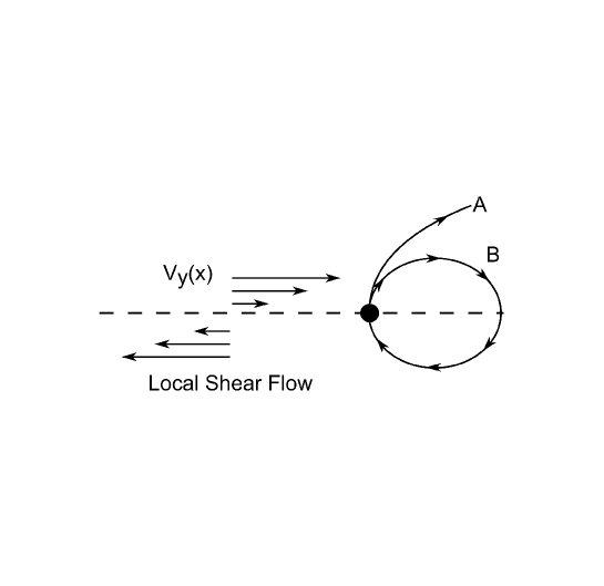
Figure 1: The stabilization mechanism in a rotating disk versus Cartesian shear flow. In shear flow, displacements are unbounded, as indicated by path A. In a disk, epicyclic motions keeps the displacement tightly bound. See text for further details.

The title of the Ji et al. (2006) paper is “Hydrodynamic turbulence cannot transport angular momentum effectively in astrophysical disks,” and that seems as good a one-sentence summary on the topic as any; their experiment is probably the final word on nonlinear Keplerian hydrodynamical shear instability. It is gratifying, therefore, that all of the difficulties encountered by Coriolis stabilization vanish when magnetic fields are taken into account. This is due to the fact that the magnetic field introduces new modes of response (shear waves) that are much less prone to Coriolis stabilization. One of these waves, the so-called “slow mode,” turns into a local instability when differential rotation is present with a weak magnetic field. This is the magnetorotational instability. To understand this porcess in more detail, it is best to begin with the fundamentals of MHD.

3 Fundamentals

In this section, a detailed derivation of the fundamental MHD equations is presented. The discussion will be more technical here than in most of the rest of the paper, but it is very important to see how the basic governing equations of the subject arise, and much of this material is not so easy to find outside of specialized treatments. I hope the reader will have the patience to read carefully through this section.

A protostellar disk is a gas of neutral particles (predominantly $H_{2}$ molecules), electrons, ions (the most important of which will generally be K⁺ and Na⁺), and dust grains. We defer to §8 a discussion of the complications due to the presence of dust grains and consider here the gas dynamical equations for mixture of neutrals, ions and atoms.

Each species (denoted by subscript $s$) is separately conserved, and obeys the mass conservation equation

$${\partial\rho_{s}\over\partial t}+\mbox{\boldmath{$\nabla$}}\mbox{\boldmath{$\cdot$}}(\rho_{s}\mbox{\boldmath{$v$}}_{s})=0$$ (1)

where $\rho_{s}$ is the mass density for species $s$ and $\mbox{\boldmath{$v$}}_{s}$ is the velocity. The flow quantities for the dominant neutral species will henceforth be presented without subscripts.

The dynamical equation for the neutral particles is

$$\rho{\partial\mbox{\boldmath{$v$}}\over\partial t}+\rho(\mbox{\boldmath{$v$}}\mbox{\boldmath{$\cdot$}}\mbox{\boldmath{$\nabla$}})\mbox{\boldmath{$v$}}=-\mbox{\boldmath{$\nabla$}}P-\rho\mbox{\boldmath{$\nabla$}}\Phi-\mbox{\boldmath{$p_{nI}$}}-\mbox{\boldmath{$p_{ne}$}}$$ (2)

where $P$ is the pressure of the neutrals, $\Phi$ the gravitational potential and $p_{nI}$ ($p_{ne}$) is the momentum exchange rate between the neutrals and the ions (electrons).

Let us examine these last two important terms in more detail. $p_{nI}$ takes the form

$$\mbox{\boldmath{$p_{nI}$}}=n\mu_{nI}(\mbox{\boldmath{$v$}}-\mbox{\boldmath{$v_{I}$}})\nu_{nI}$$ (3)

where $n$ is the number density of neutrals, and $\mu_{nI}$ is the reduced mass of an ion and neutral particle,

$$\mu_{nI}\equiv{m_{I}m_{n}\over m_{I}+m_{n}},$$ (4)

$m_{I}$ and $m_{n}$ being the ion and neutral mass respectively. $\nu_{nI}$ is the collision frequency of a neutral with a population of ions,

$$\nu_{nI}=n_{I}\langle\sigma_{nI}w_{nI}\rangle.$$ (5)

In equation (5), $n_{I}$ is the number density of ions, $\sigma_{nI}$ is the effective cross section for neutral-ion collisions, and $w_{nI}$ is the relative velocity between a neutral particle and an ion. The angle brackets represent an average over a Maxwellian distribution function for the relative velocity. (The mass appearing in this Maxwellian will of course be the reduced mass $\mu_{nI}$.) For neutral-ion scattering, we may take the cross section $\sigma_{nI}$ to be approximately geometrical, which means that the quantity in angle brackets will be proportional to $\mu_{nI}^{-1/2}$. The order of the subscripts has no particular significance for the cross section $\sigma_{nI}$ reduced mass $\mu_{nI}$ or relative velocity $w_{nI}$. But $\nu_{In}$ differs from $\nu_{nI}$: the former is proportional to the neutral density $n$, not the ion density $n_{I}$.

Putting these definitions together gives

$$\mbox{\boldmath{$p_{nI}$}}=nn_{I}\mu_{nI}\langle\sigma_{nI}w_{nI}\rangle(\mbox{\boldmath{$v$}}-\mbox{\boldmath{$v_{I}$}})$$ (6)

In accordance with Newton’s third law, this is symmetric with respect to the interchange $n\leftrightarrow I$, except for a change in sign, $\mbox{\boldmath{$p_{nI}$}}=-\mbox{\boldmath{$p_{In}$}}$. All of these considerations hold, of course, for electron-neutral scattering as well. Explicitly, we have

$$\mbox{\boldmath{$p_{ne}$}}=nn_{e}\mu_{ne}\langle\sigma_{ne}w_{ne}\rangle(\mbox{\boldmath{$v$}}-\mbox{\boldmath{$v_{e}$}})\simeq nn_{e}m_{e}\langle\sigma_{ne}w_{ne}\rangle(\mbox{\boldmath{$v$}}-\mbox{\boldmath{$v_{e}$}}).$$ (7)

The gas will be locally neutral, so that $n_{e}=Zn_{i}$ where $Z$ is the number of ionizations per ion particle. In a weakly ionized gas, $Z=1$. The reduced mass $\mu_{ne}$ may safely be set equal to the electron mass $m_{e}$. We will use the following expressions for the collision rates (Draine, Roberge, & Dalgarno 1983):

$$\langle\sigma_{nI}w_{nI}\rangle=1.9\times 10^{-9}\mbox{ cm${}^{3}$ s${}^{-1}$}$$ (8)

$$\langle\sigma_{ne}w_{ne}\rangle=10^{-15}\ (128kT/9\pi m_{e})^{1/2}=8.3\times 10^{-10}T^{1/2}\mbox{ cm${}^{3}$ s${}^{-1}$}$$ (9)

The electron-neutral collision rate is essentially the ion geometric cross section times an electron thermal velocity. (The peculiar factor of $(128/9\pi)^{1/2}$ comes from the way the electron velocity is projected, when averaged over the electron Maxwellian distribution function, along the direction of the mean ion flow.) But the ion-neutral collision rate is temperature independent, much more beholden to long range induced dipole interactions, and significantly enhanced relative to a geometrical cross section assumption. Even if the ion-neutral rate were determined only by a geometrical cross section, $|\mbox{\boldmath{$p_{nI}$}}|$ would excee $|\mbox{\boldmath{$p_{ne}$}}|$ by a factor of order $(m_{e}/\mu_{nI})^{1/2}$. In fact, the dipole enhancement of the ion-neutral cross section makes this factor yet larger.

In the astrophysical literature, it is common to write the ion-neutral momentum coupling in the form

$$\mbox{\boldmath{$p_{In}$}}=\rho\rho_{I}\gamma(\mbox{\boldmath{$v_{I}$}}-\mbox{\boldmath{$v$}}),$$ (10)

where $\gamma$ is the so-called drag coefficient,

$$\gamma\equiv{\langle\sigma_{nI}w_{nI}\rangle\over m_{I}+m_{n}}$$ (11)

and we will use this notation from here on. Numerically, $\gamma=3\times 10^{13}$ cm³ s^-1 g^-1 for astrophysical mixtures (Draine, Roberge, & Dalgarno 1983).

The dynamical equations for the ions and electrons are

$$\rho_{I}{\partial\mbox{\boldmath{$v_{I}$}}\over\partial t}+\rho_{I}\mbox{\boldmath{$v_{I}$}}\mbox{\boldmath{$\cdot$}}\mbox{\boldmath{$\nabla$}}\mbox{\boldmath{$v_{I}$}}=-\mbox{\boldmath{$\nabla$}}P_{I}-\rho_{I}\mbox{\boldmath{$\nabla$}}\Phi+Zen_{I}\left(\mbox{\boldmath{$E$}}+{\mbox{\boldmath{$\mbox{\boldmath{$v_{I}$}}$}}\over c}\mbox{\boldmath{$\times$}}\mbox{\boldmath{$B$}}\right)-\mbox{\boldmath{$p_{In}$}}$$ (12)

and

$$\rho_{e}{\partial\mbox{\boldmath{$v_{e}$}}\over\partial t}+\rho_{e}\mbox{\boldmath{$v_{e}$}}\mbox{\boldmath{$\cdot$}}\mbox{\boldmath{$\nabla$}}\mbox{\boldmath{$v_{e}$}}=-\mbox{\boldmath{$\nabla$}}P_{e}-\rho_{e}\mbox{\boldmath{$\nabla$}}\Phi-en_{e}\left(\mbox{\boldmath{$E$}}+{\mbox{\boldmath{$\mbox{\boldmath{$v_{e}$}}$}}\over c}\mbox{\boldmath{$\times$}}\mbox{\boldmath{$B$}}\right)-\mbox{\boldmath{$p_{en}$}},$$ (13)

respectively. Throughout this paper, $e$ will denote the positive charge of a proton, $4.803\times 10^{-10}$ esu. For a weakly ionized gas, the Lorentz force and collisional terms dominate in each of the latter two equations. Comparison of the magnetic and inertial forces, for example, shows that the latter are smaller than the former by the ratio of the proton or electron gyroperiod to a macroscopic flow crossing time. Thus, to an excellent degree of approximation,

$$Zen_{I}\left(\mbox{\boldmath{$E$}}+{\mbox{\boldmath{$\mbox{\boldmath{$v_{I}$}}$}}\over c}\mbox{\boldmath{$\times$}}\mbox{\boldmath{$B$}}\right)-\mbox{\boldmath{$p_{In}$}}=0,$$ (14)

and

$$-en_{e}\left(\mbox{\boldmath{$E$}}+{\mbox{\boldmath{$\mbox{\boldmath{$v_{e}$}}$}}\over c}\mbox{\boldmath{$\times$}}\mbox{\boldmath{$B$}}\right)-\mbox{\boldmath{$p_{en}$}}=0.$$ (15)

The sum of these two equations gives

$${\mbox{\boldmath{$J$}}\over c}\mbox{\boldmath{$\times$}}\mbox{\boldmath{$B$}}=\mbox{\boldmath{$p_{In}$}}+\mbox{\boldmath{$p_{en}$}}$$ (16)

where charge neutrality $n_{e}=Zn_{I}$ has been used, and we have introduced the current density

$$\mbox{\boldmath{$J$}}\equiv en_{e}(\mbox{\boldmath{$v_{I}$}}-\mbox{\boldmath{$v_{e}$}}).$$ (17)

The equation for the neutrals becomes

$$\rho{\partial\mbox{\boldmath{$v$}}\over\partial t}+\rho\mbox{\boldmath{$v$}}\mbox{\boldmath{$\cdot$}}\mbox{\boldmath{$\nabla$}}\mbox{\boldmath{$v$}}=-\mbox{\boldmath{$\nabla$}}P-\rho\mbox{\boldmath{$\nabla$}}\Phi+{\mbox{\boldmath{$J$}}\over c}\mbox{\boldmath{$\times$}}\mbox{\boldmath{$B$}}$$ (18)

Due to collisional coupling, the neutrals are subject to the magnetic Lorentz force just as though they were a gas of charged particles. It is not the magnetic force per se that changes in a neutral gas. As well shall presently see, it is the inductive properties of the gas.

Let us return to the force balance equations for the electrons:

$$-en_{e}\left(\mbox{\boldmath{$E$}}+{\mbox{\boldmath{$\mbox{\boldmath{$v_{e}$}}$}}\over c}\mbox{\boldmath{$\times$}}\mbox{\boldmath{$B$}}\right)-\mbox{\boldmath{$p_{en}$}}=0.$$ (19)

After division by $-en_{e}$, this may be expanded to

$$\mbox{\boldmath{$E$}}+{1\over c}\left[\mbox{\boldmath{$v$}}+(\mbox{\boldmath{$v_{e}$}}-\mbox{\boldmath{$v_{I}$}})+(\mbox{\boldmath{$v_{I}$}}-\mbox{\boldmath{$v$}})\right]\mbox{\boldmath{$\times$}}\mbox{\boldmath{$B$}}+{m_{e}\nu_{en}\over e}\left[(\mbox{\boldmath{$v_{e}$}}-\mbox{\boldmath{$v_{I}$}})+(\mbox{\boldmath{$v_{I}$}}-\mbox{\boldmath{$v$}})\right]=0,$$ (20)

where we have introduced the collision frequency of an electron in a population of neutrals:

$$\nu_{en}=n\langle\sigma_{ne}w_{ne}\rangle.$$ (21)

We have written the electron velocity $v_{e}$ in terms of the dominant neutral velocity $v$ and the key physical velocity differences of our problem. It has already been noted that in equation (16), $p_{en}$ is small compared with $p_{In}$, provided that the velocity difference $|\mbox{\boldmath{$v_{e}$}}-\mbox{\boldmath{$v$}}|$ is not much larger than $|\mbox{\boldmath{$v_{I}$}}-\mbox{\boldmath{$v$}}|$. In fact, when used in (20), the $p_{en}$ term in equation (16) may quite generally be dropped:

$${\mbox{\boldmath{$J$}}\over c}\mbox{\boldmath{$\times$}}\mbox{\boldmath{$B$}}\simeq\mbox{\boldmath{$p_{In}$}}.$$ (22)

It may also be shown that the final term in equation (20)

$${m_{e}\nu_{en}\over e}(\mbox{\boldmath{$v_{I}$}}-\mbox{\boldmath{$v$}}),$$

which would then be proportional to $J\times B$, becomes small compared with the third term

$${1\over c}(\mbox{\boldmath{$v_{e}$}}-\mbox{\boldmath{$v_{I}$}})\mbox{\boldmath{$\times$}}\mbox{\boldmath{$B$}},$$

also proportional to $J$$\times$$B$. Both of these rather technical claims are justified in detail in Appendix A. (In both cases, the incurred error is of order $(m_{e}/\mu_{In})^{1/2}$.) These simplifications allow us to write the electron force balance equation as

$$\mbox{\boldmath{$E$}}+{\mbox{\boldmath{$v$}}\over c}\mbox{\boldmath{$\times$}}\mbox{\boldmath{$B$}}-{\mbox{\boldmath{$J\times B$}}\over en_{e}c}-{\mbox{\boldmath{$J$}}\over\sigma_{cond}}+{\mbox{\boldmath{$(J\times B)\times B$}}\over c^{2}\gamma\rho\rho_{I}}=0,$$ (23)

where the electrical conductivity has been defined as

$$\sigma_{cond}\equiv{e^{2}n_{e}\over m_{e}\nu_{en}}$$ (24)

The associated resistivity $\eta$ is (e.g. Jackson 1975)

$$\eta={c^{2}\over 4\pi\sigma_{cond}},$$ (25)

which has units of cm² s^-1. Numerically (e.g. Blaes & Balbus 1994, Balbus & Terquem 2001):

$$\eta=234\left(n\over n_{e}\right)T^{1/2}\ \mbox{cm${}^{2}$ s${}^{-1}$}$$ (26)

Equation (23) is a general form of Ohm’s law for a moving, multiple fluid system.

Next, we make use of two of Maxwell’s equations. The first is Faraday’s induction law:

$${\mbox{\boldmath{$\nabla$}}\mbox{\boldmath{$\times$}}\mbox{\boldmath{$E$}}}=-{1\over c}{\partial\mbox{\boldmath{$B$}}\over\partial t}.$$ (27)

We substitute $E$ from equation (23) to obtain an equation for the self-induction of the magnetized fluid,

$${\partial\mbox{\boldmath{$B$}}\over\partial t}=\mbox{\boldmath{$\nabla$}}\mbox{\boldmath{$\times$}}\left[{\mbox{\boldmath{$v$}}}\mbox{\boldmath{$\times$}}\mbox{\boldmath{$B$}}-{\mbox{\boldmath{$J\times B$}}\over en_{e}}+{\mbox{\boldmath{$(J\times B)\times B$}}\over c\gamma\rho\rho_{I}}-{c\mbox{\boldmath{$J$}}\over\sigma_{cond}}\right]$$ (28)

It remains to relate the current density $J$ to the magnetic field $B$. This is accomplished by the second Maxwell equation,

$${4\pi\over c}\mbox{\boldmath{$J$}}=\mbox{\boldmath{$\nabla$}}\mbox{\boldmath{$\times$}}\mbox{\boldmath{$B$}}+{1\over c}{\partial\mbox{\boldmath{$E$}}\over\partial t}$$ (29)

The final term in the above is the displacement current, and it may be ignored. Indeed, since we have not, and will not, use the “Gauss’s Law” equation

$$\mbox{\boldmath{$\nabla$}}\mbox{\boldmath{$\cdot$}}\mbox{\boldmath{$E$}}=4\pi e(Zn_{I}-n_{e}),$$ (30)

we must not include the displacement current. In Appendix B, we show that departures from charge neutrality in $\nabla$$\cdot$$E$ and the displacement current are both small terms that contribute at the same order: $v^{2}/c^{2}$. These must both be self-consistently neglected in nonrelativisitc MHD. (The final Maxwell equation $\mbox{\boldmath{$\nabla$}}\mbox{\boldmath{$\cdot$}}\mbox{\boldmath{$B$}}=0$ adds nothing new. It is automatically satisfied by equation (27), as long as the initial magnetic field satifies this divergence free condition.) These considerations imply

$$\mbox{\boldmath{$J$}}={c\over 4\pi}\mbox{\boldmath{$\nabla$}}\mbox{\boldmath{$\times$}}\mbox{\boldmath{$B$}}$$ (31)

for use in equation (28).

To summarize, the fundamental equations of a weakly ionized fluid are mass conservation of the dominant neutrals (eq.[1])

$${\partial\rho\over\partial t}+\mbox{\boldmath{$\nabla$}}\mbox{\boldmath{$\cdot$}}(\rho\mbox{\boldmath{$v$}})=0,$$ (32)

the equation of motion (eq. [18] with [31])

$$\rho{\partial\mbox{\boldmath{$v$}}\over\partial t}+\rho\mbox{\boldmath{$v$}}\mbox{\boldmath{$\cdot$}}\mbox{\boldmath{$\nabla$}}\mbox{\boldmath{$v$}}=-\mbox{\boldmath{$\nabla$}}P-\rho\mbox{\boldmath{$\nabla$}}\Phi+{1\over 4\pi}(\mbox{\boldmath{$\nabla$}}\mbox{\boldmath{$\times$}}\mbox{\boldmath{$B$}})\mbox{\boldmath{$\times$}}\mbox{\boldmath{$B$}},$$ (33)

and the induction equation (eq. [28] with [25] and [31])

$${\partial\mbox{\boldmath{$B$}}\over\partial t}=\mbox{\boldmath{$\nabla$}}\mbox{\boldmath{$\times$}}\left[{\mbox{\boldmath{$v$}}}\mbox{\boldmath{$\times$}}\mbox{\boldmath{$B$}}-{c(\mbox{\boldmath{$\nabla\times B$}})\times\mbox{\boldmath{$B$}}\over 4\pi en_{e}}+{\mbox{\boldmath{$[(\nabla\times B)\times B]\times B$}}\over 4\pi\gamma\rho\rho_{I}}-\eta\mbox{\boldmath{$\nabla\times B$}}\right]$$ (34)

It is only natural that the reader should be a little taken aback by the sight of equation (34). Be assured that it is rarely, if ever, needed in full generality: almost always one or more terms on the right side of the equation may be discarded. When only the induction term $v$$\times$$B$ is important, we refer to this regime as ideal MHD. The three remaining terms on the right are the nonideal MHD terms.

To get a better feel for the relative importance of the nonideal MHD terms in equation (28), we denote the terms on the right side of the equation, moving left to right, as $I$ (induction), $H$ (Hall), $A$ (ambipolar diffusion), and $O$ (Ohmic resistivity). Then, the scaling of each of these terms relative to the Hall term $H$ is

$${I\over H}\sim{v\over v_{I}-v_{e}},\quad{A\over H}\sim Z{\omega_{cI}\over\gamma\rho},\quad{O\over H}\sim{\nu_{en}\over\omega_{ce}}$$ (35)

where the ion cyclotron frequency $\omega_{cI}=eB/m_{I}c$, and similarly for the electron frequency $\omega_{ce}$, with $m_{e}$ replacing $m_{I}$.

We will always be in a regime in which the presence of the induction term is not in question, i.e. the relative ion-electron drift velocity $v_{I}-v_{e}$ is always comparable to or in fact much less than $v$. More interesting is the relative importance of the nonideal terms. The explicit dependence of $A/H$ and $O/H$ in terms of the fluid properties of a cosmic gas is given in Balbus & Terquem (2001):

$${A\over H}=Z\left(9\times 10^{12}\ {\rm cm}^{-3}\over n\right)^{1/2}\left(T\over 10^{3}\,{\rm K}\right)^{1/2}\left(v_{A}\over c_{S}\right)$$ (36)

and

$${O\over H}=\left(n\over 8\times 10^{17}\ {\rm cm}^{-3}\right)^{1/2}\left(c_{S}\over v_{A}\right)$$ (37)

Here $n$ is the total number density of all particles, $T$ is the kinetic temperature, $v_{A}$ is the so-called Alfvén velocity,

$$\mbox{\boldmath{$v_{A}$}}={\mbox{\boldmath{$B$}}\over\sqrt{4\pi\rho}}$$ (38)

and $c_{S}$ is the isothermal speed of sound,

$$c_{S}^{2}=0.429{kT\over m_{p}}$$ (39)

where $k$ is the Boltzmann constant and $m_{p}$ the mass of the proton. The coefficient 0.429 corresponds to a mean mass per particle of 2.33$m_{p}$, appropriate to a molecular cosmic abundance gas.

As reassurance that the fully general nonideal MHD induction equation is not needed for our purposes, note that equations (36) and (37) imply that for all three nonideal MHD terms to be comparable, $T\sim 10^{8}$ K! Obviously this is not an issue for protostellar disks. In figure (2), we plot the domains of relative dominance of the nonideal MHD terms in the $nT$ plane. Protostellar disks are dominated by the resistive and Hall nonideal MHD terms, except in the innermost regions, where ohmic dissipation is largest, and the outermost regions, where ambipolar diffusion becomes important (Wardle 1999).

Figure 2: Parameter space for nonideal MHD. The curves correspond to the case $v_{A}/c_{S}=0.1$. (From Kunz & Balbus 2004.)

Our emphasis of the relative ordering of the nonideal terms in the induction equation should not obscure the fact that ideal MHD is often an excellent approximation, even when the ionization fraction is $\ll 1$. For example, the ratio of the ideal inductive term to the ohmic loss term is given by the Lundquist number

$$\mathbb{L}={v_{A}L\over\eta}$$ (40)

where $L$ is a characteristic gradient length scale. To orient ourselves, let us set $L=0.1R$, where $R$ is the radial location in the disk. Then $\mathbb{L}$ is given by

$$\mathbb{L}\simeq 2.5(n_{e}/n)(v_{A}/c_{S})R_{cm},$$

$R_{cm}$ being the radius in centimeters. In other words, the critical ionization fraction at which $\mathbb{L}=1$ is about

$$(n_{e}/n)_{crit}=0.4(c_{S}/v_{A})R_{cm}^{-1}\sim 10^{-13}(c_{S}/10v_{A})$$

at $R=1$ AU. The actual nebular ionization fraction at this location may be above or below this during the course of the solar systems evolution, but the point worth noting here is that $R_{cm}$ is a large number for a protostellar disk, whatever the ionization source! Ionization fractions far, far below unity can render an astrophysical gas a near perfect electrical conductor. It therefore makes a great deal of sense to begin by examining the behavior of an ideal MHD fluid.

4 Ideal MHD

The fundamental equations of ideal (single-fluid) MHD are mass conservation (1)

$${\partial\rho\over\partial t}+\mbox{\boldmath{$\nabla$}}\mbox{\boldmath{$\cdot$}}(\rho\mbox{\boldmath{$v$}})=0$$ (41)

the dynamical equation of motion

$${\partial\mbox{\boldmath{$v$}}\over\partial t}+(\mbox{\boldmath{$v$}}\mbox{\boldmath{$\cdot$}}\mbox{\boldmath{$\nabla$}})\mbox{\boldmath{$v$}}=-{1\over\rho}\mbox{\boldmath{$\nabla$}}\left(P+{B^{2}\over 8\pi}\right)-\mbox{\boldmath{$\nabla$}}\Phi+({\mbox{\boldmath{$B$}}\over 4\pi}\mbox{\boldmath{$\cdot$}})\mbox{\boldmath{$\nabla$}}\mbox{\boldmath{$B$}}$$ (42)

where $\Phi$ is the (central) gravitational potential function, and our newly simplified induction equation

$${\partial\mbox{\boldmath{$B$}}\over\partial t}=\mbox{\boldmath{$\nabla$}}\mbox{\boldmath{$\times$}}(\mbox{\boldmath{$v$}}\mbox{\boldmath{$\times$}}\mbox{\boldmath{$B$}})$$ (43)

We shall work in a standard cylindrical coordinate system $(R,\phi,z)$, where $R$ is the radius, $\phi$ the azimuthal angle, and $z$ the vertical coordinate. In these coordinates, the three components of the equation of motion are are

$$\left[{\partial\ \over\partial t}+\mbox{\boldmath{$v$}}\mbox{\boldmath{$\cdot$}}\mbox{\boldmath{$\nabla$}}\right]v_{R}-{v^{2}_{\phi}\over R}=-{1\over\rho}{\partial\ \over\partial R}\left(P+{B^{2}\over 8\pi}\right)-{\partial\Phi\over\partial R}+{\mbox{\boldmath{$B$}}\over 4\pi\rho}\mbox{\boldmath{$\cdot$}}\mbox{\boldmath{$\nabla$}}B_{R}-{B^{2}_{\phi}\over 4\pi\rho R},$$ (44)

$$\left[{\partial\ \over\partial t}+\mbox{\boldmath{$v$}}\mbox{\boldmath{$\cdot$}}\mbox{\boldmath{$\nabla$}}\right](Rv_{\phi})=-{1\over\rho}{\partial\ \over\partial\phi}\left(P+{B^{2}\over 8\pi}\right)+{\mbox{\boldmath{$B$}}\over 4\pi\rho}\mbox{\boldmath{$\cdot$}}\mbox{\boldmath{$\nabla$}}(RB_{\phi}),$$ (45)

$$\left[{\partial\ \over\partial t}+\mbox{\boldmath{$v$}}\mbox{\boldmath{$\cdot$}}\mbox{\boldmath{$\nabla$}}\right]v_{z}=-{1\over\rho}{\partial\ \over\partial z}\left(P+{B^{2}\over 8\pi}\right)-{\partial\Phi\over\partial z}+{\mbox{\boldmath{$B$}}\over 4\pi\rho}\mbox{\boldmath{$\cdot$}}\mbox{\boldmath{$\nabla$}}B_{z},$$ (46)

and the three components of the induction equation are

$$\left[{\partial\ \over\partial t}+\mbox{\boldmath{$v$}}\mbox{\boldmath{$\cdot$}}\mbox{\boldmath{$\nabla$}}\right]B_{R}=-B_{R}\mbox{\boldmath{$\nabla$}}\mbox{\boldmath{$\cdot$}}\mbox{\boldmath{$v$}}+\mbox{\boldmath{$B$}}\mbox{\boldmath{$\cdot$}}\mbox{\boldmath{$\nabla$}}v_{R}$$ (47)

$$\left[{\partial\ \over\partial t}+\mbox{\boldmath{$v$}}\mbox{\boldmath{$\cdot$}}\mbox{\boldmath{$\nabla$}}\right]{B_{\phi}\over R}=-{B_{\phi}\over R}\mbox{\boldmath{$\nabla$}}\mbox{\boldmath{$\cdot$}}\mbox{\boldmath{$v$}}+\mbox{\boldmath{$B$}}\mbox{\boldmath{$\cdot$}}\mbox{\boldmath{$\nabla$}}\left(v_{\phi}\over R\right)$$ (48)

$$\left[{\partial\ \over\partial t}+\mbox{\boldmath{$v$}}\mbox{\boldmath{$\cdot$}}\mbox{\boldmath{$\nabla$}}\right]B_{z}=-B_{z}\mbox{\boldmath{$\nabla$}}\mbox{\boldmath{$\cdot$}}\mbox{\boldmath{$v$}}+\mbox{\boldmath{$B$}}\mbox{\boldmath{$\cdot$}}\mbox{\boldmath{$\nabla$}}v_{z}$$ (49)

For many problems of interest, an important simplification can be made to these equations. The essence of rotational dynamics is local. Imagine going to a location $R_{0}$ in the disk. The Keplerian angular velocity $\Omega$ at $R=R_{0}$ is $\Omega_{0}$. We hold $\Omega_{0}$ fixed but allow $R_{0}$ to become arbitrarily large. Thus, $v_{\phi}(R_{0})$ is unbounded, but $v_{\phi}/R_{0}=\Omega_{0}$ is finite.

Next, we introduce local coordinates $(x,\alpha,z)$ defined by

$$R=R_{0}+x,\qquad x\ll R_{0},$$ (50)

$$\alpha=\phi-\Omega_{0}t\ll\pi$$ (51)

and $z$ is unchanged. We will formally introduce a new coordinate $t^{\prime}=t$. This is desirable because we wish to take a time derivative at constant $x,y,z$, not at constant $R,\phi,z$. In fact,

$${\partial\ \over\partial t^{\prime}}={\partial\ \over\partial t}+\Omega_{0}{\partial\over\partial\alpha}$$ (52)

Partial derivatives with respect to $R$ and $\phi$ become partial derivatives with respect to $x$ and $\alpha$ respectively. The Lagrangian derivative

$${\partial\ \over\partial t}+\mbox{\boldmath{$v$}}\mbox{\boldmath{$\cdot$}}\mbox{\boldmath{$\nabla$}}$$ (53)

becomes

$${\partial\ \over\partial t^{\prime}}+(\mbox{\boldmath{$v$}}-R\Omega_{0}\mbox{\boldmath{$e_{\phi}$}})\mbox{\boldmath{$\cdot$}}\mbox{\boldmath{$\nabla$}}$$ (54)

(The $\nabla$ operator now formally involves $x$ and $\alpha$ derivatives.) This transformation suggests that we introduce a new azimuthal velocity,

$$w_{\alpha}=v_{\phi}-R\Omega_{0}$$ (55)

and for notational consistency we will use $w_{x}$ and $w_{z}$ for the radial and vertical velocities, though they are identical to $v_{R}$ and $v_{z}$.

In the local approximation, we assume that the magnitude $w$ is much smaller than the (formally infinite) rotation velocity, and that $w$, the Alfven speed $v_{A}$, and the thermal velocity $(P/\rho)^{1/2}$ are comparable in magnitude. In the limit $R_{0}\rightarrow\infty$, the radial equation becomes

$$\left[{\partial\ \over\partial t^{\prime}}+\mbox{\boldmath{$w$}}\mbox{\boldmath{$\cdot$}}\mbox{\boldmath{$\nabla$}}\right]w_{R}-2\Omega_{0}w_{\phi}=R(\Omega^{2}_{0}-\Omega^{2}_{K})-{1\over\rho}{\partial\ \over\partial x}\left(P+{B^{2}\over 8\pi}\right)+{\mbox{\boldmath{$B$}}\over 4\pi\rho}\mbox{\boldmath{$\cdot$}}\mbox{\boldmath{$\nabla$}}B_{R},$$ (56)

where the Keplerian angular velocity at $R$ satisfies

$$R\Omega^{2}_{K}={\partial\Phi\over\partial R}$$ (57)

Expanding to first order in $R$,

$$R(\Omega^{2}_{0}-\Omega^{2}_{K})=-x{d\Omega^{2}_{K}\over dR}=3\Omega^{2}_{0}$$ (58)

The final form of the equation is

$$\left[{\partial\ \over\partial t}+\mbox{\boldmath{$w$}}\mbox{\boldmath{$\cdot$}}\mbox{\boldmath{$\nabla$}}\right]w_{x}-2\Omega w_{y}=3\Omega^{2}x-{1\over\rho}{\partial\ \over\partial x}\left(P+{B^{2}\over 8\pi}\right)+{\mbox{\boldmath{$B$}}\over 4\pi\rho}\mbox{\boldmath{$\cdot$}}\mbox{\boldmath{$\nabla$}}B_{x},$$ (59)

where we have dropped the subscript $0$ and the prime ^′. The vector components $x,y,z$ refer to the quasi-Cartesian system $dx=dR$, $dy=Rd\alpha$, and $dz$ as before. (See fig. 2.) When non-Keplerian disks are considered, $3\Omega^{2}$ should be replaced by $d\Omega^{2}/d\ln R$.

The transformed azimuthal ($y$) equation is

$$\left[{\partial\ \over\partial t}+\mbox{\boldmath{$w$}}\mbox{\boldmath{$\cdot$}}\mbox{\boldmath{$\nabla$}}\right]w_{y}-2\Omega w_{x}=-{1\over\rho}{\partial\ \over\partial y}\left(P+{B^{2}\over 8\pi}\right)+{\mbox{\boldmath{$B$}}\over 4\pi\rho}\mbox{\boldmath{$\cdot$}}\mbox{\boldmath{$\nabla$}}B_{y},$$ (60)

and the $z$ equation is

$$\left[{\partial\ \over\partial t}+\mbox{\boldmath{$w$}}\mbox{\boldmath{$\cdot$}}\mbox{\boldmath{$\nabla$}}\right]w_{z}=-{\partial\Phi\over\partial z}-{1\over\rho}{\partial\ \over\partial z}\left(P+{B^{2}\over 8\pi}\right)+{\mbox{\boldmath{$B$}}\over 4\pi\rho}\mbox{\boldmath{$\cdot$}}\mbox{\boldmath{$\nabla$}}B_{z},$$ (61)

The mass conservation and induction equations, like the $z$ equation of motion, show no change of form in these corotating coordinates:

$${\partial\rho\over\partial t}+\mbox{\boldmath{$\nabla$}}\mbox{\boldmath{$\cdot$}}(\rho\mbox{\boldmath{$w$}})=0,$$ (62)

$${\partial\mbox{\boldmath{$B$}}\over\partial t}=\mbox{\boldmath{$\nabla$}}\mbox{\boldmath{$\times$}}(\mbox{\boldmath{$w$}}\mbox{\boldmath{$\times$}}\mbox{\boldmath{$B$}})$$ (63)

To summarize, we have transformed our general equations into a coordinate frame rotating at the Keplerian angular velocity $\Omega_{K}(R_{0})$, restricting the spatial domain to a small neighborhood around a particular fluid element. The rotational dynamics appears in the form of a Coriolis force $-2\mbox{\boldmath{$\Omega$}}\mbox{\boldmath{$\times$}}\mbox{\boldmath{$w$}}$, and a centrifugal force that cancels the main gravitational force, leaving the residual tidal term $3\Omega^{2}x$. These simplified local equations, which are the magnetized version of what is known as the Hill system, retain a rich dynamical content. This includes the full development of MHD turbulence.

4.1 Magnetorotational Instability

Let us apply equations (56)- (63) to the study of the paths of fluid elements departing from the origin $x=y=z=0$. These Lagrangian displacements are in the $xy$ orbital plane, and depend only upon $z$. We will ignore vertical stratification here, so that the equilibrium is $z$ independent. Thus, we may assume a spatial dependence of $e^{ikz}$ for the perturbed fluid elements.

We assume a very simple equilibrium magnetic field: a constant vertical component $B$, no components in the orbital $xy$ plane. If the displacement vector of an element of fluid in the $xy$ plane is $\xi$, then the perturbed magnetic field at given location is

$$\delta\mbox{\boldmath{$B$}}=\mbox{\boldmath{$\nabla$}}\mbox{\boldmath{$\times$}}(\mbox{\boldmath{$\xi$}}\mbox{\boldmath{$\times$}}\mbox{\boldmath{$B$}})$$ (64)

This result, which is true quite generally, is lengthy to prove by a direct assault, but can be intuited rather easily. The left side of the exact equation (63) may be written $\delta\mbox{\boldmath{$B$}}/\delta t$, the change in $B$ at fixed location divided by the change in time. In the equilibrium state this is zero. Imagine perturbing this pure state by giving each fluid an additional finite velocity $U$, but letting it act only for an infinitesimal time $\delta t$. Then

$$\delta\mbox{\boldmath{$B$}}=\mbox{\boldmath{$\nabla$}}\mbox{\boldmath{$\times$}}(\mbox{\boldmath{$w$}}\,\delta t\mbox{\boldmath{$\times$}}\mbox{\boldmath{$B$}})+\mbox{\boldmath{$\nabla$}}\mbox{\boldmath{$\times$}}(\mbox{\boldmath{$U$}}\,\delta t\mbox{\boldmath{$\times$}}\mbox{\boldmath{$B$}})=0+\mbox{\boldmath{$\nabla$}}\mbox{\boldmath{$\times$}}(\mbox{\boldmath{$\xi$}}\mbox{\boldmath{$\times$}}\mbox{\boldmath{$B$}})$$ (65)

where $\mbox{\boldmath{$\xi$}}=\mbox{\boldmath{$U$}}\delta t$ is the displacement of the fluid relative to its equilibrium path. This result is perhaps more clear in integral form. If we integrate over a surface $A$ and use Stokes Theorem, there obtains

$$\int\delta\mbox{\boldmath{$B$}}\mbox{\boldmath{$\cdot$}}\mbox{\boldmath{$dA$}}=\int\mbox{\boldmath{$(\xi\times B)\cdot ds$}}\equiv\int\mbox{\boldmath{$(ds\times\xi)\cdot B$}},$$ (66)

where $ds$ is a vector line element on the curve bounding $A$. This states that whatever explicit change in magnetic flux there is through $A$ as the surface is displaced by $\xi$, it is precisely compensated by the gain (or loss) of magnetic flux through of the side of the cylinder (elemental area $ds\times\xi$) swept out by $A$. This is just a round about way of saying that the magnetic flux through $A$ is conserved when moving with the fluid itself.

For the problem at hand,

$$\delta\mbox{\boldmath{$B$}}=\mbox{\boldmath{$\nabla$}}\mbox{\boldmath{$\times$}}(\mbox{\boldmath{$\xi$}}\mbox{\boldmath{$\times$}}\mbox{\boldmath{$B$}})=i\mbox{\boldmath{$k$}}\mbox{\boldmath{$\times$}}(\mbox{\boldmath{$\xi$}}\mbox{\boldmath{$\times$}}\mbox{\boldmath{$B$}})=i(\mbox{\boldmath{$k\cdot B$}})\mbox{\boldmath{$\xi$}},$$ (67)

since $\mbox{\boldmath{$k\cdot\xi$}}=0$. The magnetic term in equations (56) and (60) is

$${1\over 4\pi\rho}\mbox{\boldmath{$B$}}\mbox{\boldmath{$\cdot$}}\mbox{\boldmath{$\nabla$}}\delta\mbox{\boldmath{$B$}}=-{(\mbox{\boldmath{$k\cdot B$}})^{2}\over 4\pi\rho}\mbox{\boldmath{$\xi$}}\equiv-(\mbox{\boldmath{$k\cdot v_{A}$}})^{2}\mbox{\boldmath{$\xi$}}$$ (68)

We have introduced the so-called Alfvén velocity

$$\mbox{\boldmath{$v_{A}$}}={\mbox{\boldmath{$B$}}\over\sqrt{4\pi\rho}}$$ (69)

whose physical interpretation we discuss below. For the moment, note that the magnetic force is like tension or a spring: it is always restoring, and proportional to the displacement.

In equations (56) and (60), the derivative

$${D\ \over Dt}\equiv{\partial\over\partial t}+\mbox{\boldmath{$v$}}\mbox{\boldmath{$\cdot$}}\mbox{\boldmath{$\nabla$}}$$

is just the time derivative following a fluid element, so that we will write $D\mbox{\boldmath{$w$}}/Dt={\mbox{\boldmath{$\ddot{\xi}$}}}$, and of course $\mbox{\boldmath{$w$}}={\mbox{\boldmath{$\dot{\xi}$}}}$. Finally, we will allow for the possibility of non-Keplerian rotation. The equations of motion for the fluid element displacements $\xi_{x}$ and $\xi_{y}$ are then

$$\ddot{\xi}_{x}-2\Omega\dot{\xi}_{y}=-\left[{d\Omega^{2}\over d\ln R}+(kv_{A})^{2}\right]\xi_{x}$$ (70)

$$\ddot{\xi}_{y}+2\Omega\dot{\xi}_{x}=-(kv_{A})^{2}\xi_{y}$$ (71)

These are a simple set of coupled linear equations with time-dependent solutions of the form $e^{i\omega t}$. Without loss of generality, we take $\omega>0$. In the absence of rotation, the equations decouple completely and one finds

$$\omega=|kv_{A}|$$ (72)

These are waves that travel along the magnetic field lines with group and phase velocity $v_{A}$, exactly like waves on a string. These so-called Alfvén waves are thus simple, nondipersive, incompressible disturbances.

On the other hand, in the absence of rotation, we find

$$\omega^{2}=4\Omega^{2}+{d\Omega^{2}\over d\ln R}\equiv\kappa^{2}$$ (73)

$\kappa^{2}$ is known as the epicyclic frequency. In most astrophysical applications, $\Omega$ decreases radially outwards and $\kappa<4\Omega^{2}$. The fluid dispacements for this mode execute ellptical with a major to minor axis ratio of $\kappa/2\Omega$. The major axis lies along the azimuthal direction. The sense of the rotation around the ellipse is retrograde, opposite to the sense of $\Omega$. These paths are known as epicycles. Epicyclic motion corresponds to the first order departure from circular orbits for simple planetary motion.

The full dispersion relation resulting from equations (70) and (71) is more complicated than one might have expected:

$$\omega^{4}-[\kappa^{2}+2(kv_{A})^{2}]\omega^{2}+(kv_{A})^{2}\left[(kv_{A})^{2}+{d\Omega^{2}\over d\ln R}\right]=0$$ (74)

This is clearly not just a matter of adding Alfvénic and epicylic motion in quadrature, something new is going on. The dispersion relation is a simple quadratic equation in $\omega^{2}$, and it is straightforward to show that this quantity must be real. Stability may then be investigated by passing through the point $\omega^{2}\rightarrow 0$. Therefore, marginal instability corresponds to

$$(kv_{A})^{2}+{d\Omega^{2}\over d\ln R}=0$$ (75)

and instability is present when

$${d\Omega^{2}\over d\ln R}<0.$$ (76)

Of course, this condition is nearly universally satisfied for any type of astrophysical disk. This is the simplest manifestation of the magnetorotational instability, or MRI.

4.2 Physical Interpretation

The equations of motion (70) and (71) have a very simple mechanical analogue: they are exactly the equations of two point masses in orbit around a central body, bound together by a spring of frequency $kv_{A}$ (Balbus & Hawley 1992).

This mechanical analogy immediately offers a physical explanation of the MRI (see figure [3]). Two masses are connected by a spring, an inner mass $m_{i}$ and an outer mass $m_{o}$. The mass $m_{i}$ orbits faster than the outer mass $m_{o}$, causing the spring to stretch. The spring pulls backwards on $m_{i}$ and forwards on $m_{o}$. The negative torque on $m_{i}$ causes it to lose angular momentum and sink, while the positive torque on $m_{o}$ causes it to gain angular momentum and rise. Thus, even though the spring nominally supplies an attractive force, in a rotating frame this drives the masses apart. The continued stretching of the spring just makes matters worse, and the process runs away. The mass with the higher angular momentum obtains yet more, the mass with less angular momentum loses what little it has. It is the “same old story” in a dynamical context: the rich get richer and the poor get poorer.

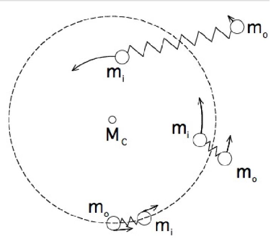
Figure 3: The magnetorotational instability. Magnetic fields in a disk bind fluid elements precisely as though they were masses in orbit connected by a spring. The inner element $m_{i}$ orbits faster than the outer element $m_{o}$, and the spring causes a net transfer of angular momentum from $m_{i}$ to $m_{o}$. This transfer is unstable, as described in the text. The inner mass continues to sink, whereas the outer mass rises farther outward. (Figure courtesy of H. Ji.)

In a protostellar disk, it is the magnetic tension force that plays the role of the spring, and the two masses are any two fluid elements tethered by the field line. The linear phase of the instability is the exponentially growing separation of the displaced fluid elements, which is followed by the nonlinear mixing of gas parcels from different regions of the disk. The mixing seems to lead to something resembling a classical turbulent cascade, though the details of this process, with different viscous and resistive dissipation scales, remain to be fully understood.

Notice that angular momentum transport is not something that happens as a consequence of the nonlinear development of the MRI, it is the essence of the MRI even in its linear phase. The very act of transporting angular momentum from the inner to outer fluid elements via a magnetic couple is a spontaneously unstable process.

4.3 General Adiabatic Disturbances

If $\Omega$ is a function only of cylindrical radius $R$, then for general magnetic field geometries, local incompressible WKB disturbances with space-time dependence

$$\delta X\sim\exp(ik_{R}R+ik_{z}z-i\omega t)$$ (77)

where $\delta X$ is the Eulerian perturbation of any flow quantity, satisfy the following set of linearized dynamical equations:

$$k_{R}\delta v_{R}+k_{z}\delta v_{z}=0,$$ (78)

$$-i\omega\delta v_{R}-2\Omega\delta v_{\phi}+i{k_{R}\over\rho}\left[\delta P+{\mbox{\boldmath{$B\cdot\delta B$}}\over 4\pi}\right]-i{\mbox{\boldmath{$k\cdot B$}}\over 4\pi\rho}\delta B_{R}=0,$$ (79)

$$-i\omega\delta v_{\phi}+{\kappa^{2}\over 2\Omega}\delta v_{R}-i{\mbox{\boldmath{$k\cdot B$}}\over 4\pi\rho}\delta B_{R}=0,$$ (80)

$$-i\omega\delta v_{z}+i{k_{z}\over\rho}\left[\delta P+{\mbox{\boldmath{$B\cdot\delta B$}}\over 4\pi}\right]-i{\mbox{\boldmath{$k\cdot B$}}\over 4\pi\rho}\delta B_{z}=0.$$ (81)

The linearized induction equations are

$$-i\omega\delta B_{R}-i(\mbox{\boldmath{$k\cdot B$}})\delta v_{R}=0,$$ (82)

$$-i\omega\delta B_{\phi}-\delta B_{R}{d\Omega\over d\ln R}-i(\mbox{\boldmath{$k\cdot B$}})\delta v_{\phi}=0,$$ (83)

$$-i\omega\delta B_{z}-i(\mbox{\boldmath{$k\cdot B$}})\delta v_{z}=0.$$ (84)

Finally, the entropy equation is

$$i\omega\gamma{\delta\rho\over\rho}+\delta v_{z}{\partial\ln P\rho^{-\gamma}\over\partial z}=0,$$ (85)

where $\gamma$ is the adiabatic index (not to be confused with the collsion rate). We have ignored background radial gradients in the entropy and pressure, but retained their vertical gradients, in accordance with the assumption of a thin disk.

This set of linearized equations leads to the dispersion relation (Balbus & Hawley 1991)

$$\left(k^{2}\over k_{z}^{2}\right)\tilde{\omega}^{4}-\left[\kappa^{2}+\left(k_{R}\over k_{z}\right)^{2}N^{2}\right]\tilde{\omega}^{2}-4\Omega^{2}(\mbox{\boldmath{$k\cdot v_{A}$}})^{2}=0.$$ (86)

Here

$$\tilde{\omega}^{2}=\omega^{2}-(\mbox{\boldmath{$k\cdot v_{A}$}})^{2},\quad k^{2}=k_{z}^{2}+k_{R}^{2},$$ (87)

and

$$N^{2}=-{1\over\gamma\rho}{\partial P\over\partial z}{\partial\ln P\rho^{-\gamma}\over\partial z}.$$ (88)

$N$ is known as the Brunt-Väisälä frequency. It is the natural frequency at which a vertically displaced fluid element would oscillate in the disk due to buoyancy forces. In general there is also a contribution due to radial gradients as well (Balbus & Hawley 1991), but this usually may be ignored in a rotationally supported (supersonic orbital speed) disk. Without any magnetic field, the dispersion relation becomes

$$\omega^{2}=(k_{z}/k)^{2}\kappa^{2}+(k_{R}/k)^{2}N^{2}$$ (89)

Since the displacement of the fluid element is incompressible, the wave number ratio $k_{z}/k$ is a measure of the radial displacement, whereas $k_{R}/k$ is a measure of the vertical displacement. There is no instability in this case, only a wavelike response due to the restoring Corilois and buoyant forces.

Notice that $N$ vanishes in the disk plane by symmetry, it affects only the behavior of disturbances at least one scale height or so above $z=0$. Moreover, the actual value of $N$ is likely to be determined by radiative diffusion processes in the vertical direction. The radiation requires a source, which in disks is the turbulence we are trying to explain in the first place! (In protostellar disks, external heating of the upper layers is also a source of departure from adiabatic behavior.)

The other limit of interest is $k_{R}=0$, which returns us to the dispersion relation of the previous section. (The expression $kv_{A}$ should of course be replaced by $k\cdot v_{A}$.) This is fortunate because it can be shown (Balbus & Hawley 1992) that the most rapidly growing modes are displacements in the plane of the disk with $k_{R}=0$. Since it is the differential rotation that ultimately destabilizes, it is very sensible that these displacements, which most effectively sample the differential rotation, are the most unstable. For a Keplerian rotation profile, it may be directly computed from the dispersion relation that the wave number of maximum growth is given by

$$\mbox{\boldmath{$k\cdot v_{A}$}}=(\sqrt{15}/4)\Omega\quad{\rm(wavenumber\ of\ maximum\ growth)},$$ (90)

or $0.97\Omega$. By comparison, the largest unstable wavelength (i.e., smallest unstable wave number) has a value of $1.73\Omega$ for $k\cdot v_{A}$. The maximum growth rate is

$$|\omega|=(3/4)\Omega\quad{\rm(maximum\ growth\ rate)}$$ (91)

This is a very large growth rate, with amplitudes growing at a rate of $\exp(3\pi/2)\sim 111$ per orbit.

4.4 Angular Momentum Transport

The azimuthal equation of motion (45) may be written

$${\partial(\rho Rv_{\phi})\over\partial t}+\mbox{\boldmath{$\nabla$}}\mbox{\boldmath{$\cdot$}}\left[R\left(\rho\mbox{\boldmath{$v$}}v_{\phi}-\rho\mbox{\boldmath{$v_{A}$}}v_{A\phi}+\left(P+{B^{2}\over 8\pi}\right)\mbox{\boldmath{$e_{\phi}$}}\right)\right]=0,$$ (92)

where $v_{A\phi}$ is the azimuthal component of the Alfvén velocity. This is an equation for angular momentum conservation, with angular momentum density $\rho Rv_{\phi}$, and an azimuthally averaged flux of

$$\mbox{\boldmath{$F_{J}$}}=\langle R\left(\rho\mbox{\boldmath{$v$}}v_{\phi}-\rho\mbox{\boldmath{$v_{A}$}}v_{A\phi}\right)\rangle$$ (93)

In protostellar disks, we are interested in the radial transport of angular momentum,

$$F_{JR}=R\rho(v_{R}v_{\phi}-v_{AR}v_{A\phi})$$ (94)

It is most instructive to begin with the simple case of linear instability in a uniform, vertical magnetic field. What is the lowest order flux that results from these exponentially growing modes? In equilibrium, $v_{R}$ and the Alfven velocities vanish. The linear pertubation of the radial velocity at a given spatial location (a so-called Eulerian perturbation) will be denoted $\delta v_{R}$. Let the radial displacement $\xi_{R}$ of a fluid element from its equilibrium location be given by

$$\xi_{R}=ae^{\gamma t}\cos(kz)$$ (95)

where $\gamma$ and $k$ correspond to the maximum growth rate and its associated wave number, and $a$ is a slowly varying amplitude. Then

$$\delta v_{R}=\dot{\xi}_{R}=\gamma\xi_{R}$$ (96)

The azimuthal velocity $v_{\phi}$ consists of an unperturbed Keplerian velocity $R\Omega$ plus a linear perturbation $\delta v_{\phi}$. The product of $\delta v_{R}$ and $\Omega$ contributes zero when a height integration is performed because of the cosine factor, so we must consider the direct product $\delta v_{R}\times\delta v_{\phi}$ to obtain the lowest order contribution. In calculating $\delta v_{\phi}$, note that

$$\delta v_{\phi}=\dot{\xi}_{\phi}-\xi_{R}{d\Omega\over d\ln R}$$ (97)

The subtraction is needed to eliminate the change in velocity a displaced fluid element would make even if there were no physical change in the rotation velocity at the new radial location: the actual change in velocity $\delta v_{\phi}$ is due to the change in $\dot{\xi}_{\phi}$ the displaced fluid element makes in excess of $\xi_{R}d\Omega/d\ln R$. Equation (70) then gives

$$\delta v_{\phi}=\dot{\xi}_{\phi}-\xi_{R}{d\Omega\over d\ln R}=\left(\gamma^{2}+k^{2}v_{A}^{2}\over 2\Omega\right)\xi_{R}$$ (98)

and therefore the velocity contribution to the angular momentum flux is

$$\langle\delta v_{R}\delta v_{\phi}\rangle={\gamma\over 2\Omega}(\gamma^{2}+k^{2}v_{A}^{2})\langle\xi_{R}^{2}\rangle$$ (99)

Not surprisingly, it is positive (outward).

To calculate the magnetic field correlation, we use equation (67) to go between magnetic field fluctuations and displacements. Then, using (71), we find

$$\xi_{\phi}=-{2\omega\gamma\over\gamma^{2}+k^{2}v_{A}^{2}}\,\xi_{R}$$ (100)

from which it follows, among other things, that $\dot{\xi}_{\phi}$ and $\delta v_{\phi}$ have opposite signs. Hence

$${\langle\delta B_{R}\delta B_{\phi}\rangle\over 4\pi\rho}=-{2\Omega k^{2}v_{A}^{2}\gamma\over\gamma^{2}+k^{2}v_{A}^{2}}\langle\xi_{R}^{2}\rangle$$ (101)

Therefore

$$\langle\delta v_{R}\delta v_{\phi}-{\delta B_{R}\delta B_{\phi}\over 4\pi\rho}\rangle={\gamma\over 2\Omega}\left[(\gamma^{2}+k^{2}v_{A}^{2})^{2}+4\Omega^{2}k^{2}v_{A}^{2}\over\gamma^{2}+k^{2}v_{A}^{2}\right]\langle\xi_{R}^{2}\rangle$$ (102)

Using the dispersion relation (74) to simplify this a bit, our expression for the radial angular momentum flux is

$$F_{JR}=\rho R\ {\gamma\over 2\Omega}\left[{8\Omega^{2}k^{2}v_{A}^{2}\over\gamma^{2}+k^{2}v_{A}^{2}}-\kappa^{2}\right]\langle\xi_{R}^{2}\rangle$$ (103)

Finally, integrating over height and defining the effective surface density $\Sigma$ by

$$\int\rho\langle\xi_{R}^{2}\rangle\,dz=\Sigma a^{2}e^{2\gamma t}/2,$$ (104)

the angular momentum flux for the most rapidly growing mode is found to be

$$F_{JR}={3R\Sigma\over 4}\Omega^{2}a^{2}e^{2\gamma t}$$ (105)

This result bears some commentary. First, the radial flux is always positive for any unstable mode, not just the most rapidly growing. This, as we shall see, is a direct consequence of energy conservation: energy is extracted from the differential rotation to the fluctuations only if the radial angular momentum flux is positive. Next, note that there is an outward angular momentum flux only to the extent that there is a correlation in the velocity fluctuations. This is also true in turbulent flows, and everything that we have done in this section goes through in much the same way if the fluctuations are turbulent as opposed to wavelike. The important physical point is that an instability that leads to turbulence need not lead to enhanced angular momentum transport. Only turbulence with strongly correlated velocity fields does this. Strong correlations, in turn, are necessary to extract energy from differential rotation. This is indeed the free energy source of shear-driven turbulence, but not any form of turbulence.

This point was made in Stone & Balbus (1996), in which the angular momentum transport resulting from convective instability was studied. The angular momentum was tiny in magnitude and inwardly directed: it had the “wrong” sign. Disk intabilities based on adverse thermal gradients do not, in general, lead to systematically large outward transfers of angular momentum. When it comes to angular momentum transport, not all turbulence is equivalent.

4.5 Diffusion of a Scalar

A classical problem in protostellar disk theory is to understand how dust particles are mixed with the gas. The fact that the MRI leads to vigorous radial angular momentum transport suggests that other quantities may be transported as well. In this section, we will give an argument that shows that the radial diffusion of angular momentum is indeed closely related to the radial transport of a conserved scalar quantity, say $Q$. Assume that $Q$ is a fluid element label and satisfies an equation of the form

$$\left({\partial\ \over\partial t}+\mbox{\boldmath{$v$}}\mbox{\boldmath{$\cdot$}}\mbox{\boldmath{$\nabla$}}\right)Q=0$$ (106)

Then,

$${\partial Q\over\partial t}+\mbox{\boldmath{$\nabla$}}\mbox{\boldmath{$\cdot$}}(\mbox{\boldmath{$v$}}Q)-Q\mbox{\boldmath{$\nabla$}}\mbox{\boldmath{$\cdot$}}\mbox{\boldmath{$v$}}=0.$$ (107)

Using mass conservation, this implies

$${\partial Q\over\partial t}+\mbox{\boldmath{$\nabla$}}\mbox{\boldmath{$\cdot$}}(\mbox{\boldmath{$v$}}Q)+Q{D\ln\rho\over Dt}=0,$$ (108)

where

$${D\ \over Dt}=\left({\partial\ \over\partial t}+\mbox{\boldmath{$v$}}\mbox{\boldmath{$\cdot$}}\mbox{\boldmath{$\nabla$}}\right)$$ (109)

Simplifying the equation for $Q$, we obtain

$${\partial(\rho Q)\over\partial t}+\mbox{\boldmath{$\nabla$}}\mbox{\boldmath{$\cdot$}}(\rho\mbox{\boldmath{$v$}}Q)=0,$$ (110)

which looks very much like the angular momentum conservation equation (92). In a similar way, there will be a turbulent $Q$-flux given by

$$F_{Q}=\rho\langle\delta\mbox{\boldmath{$v$}}\delta Q\rangle$$ (111)

Since $Q$ is conserved as we follow a fluid element, the so-called Lagrangian perturbation $\Delta Q$, defined by

$$\Delta Q=\delta Q+\mbox{\boldmath{$\xi$}}\mbox{\boldmath{$\cdot$}}\mbox{\boldmath{$\nabla$}}Q$$ (112)

must vanish. This is because $\Delta Q$ is constructed to be the change in $Q$ following a fluid element as it is displaced by a small distance $\xi$, and such changes must vanish since by definition $Q$ is does not change along fluid element paths. Hence, our expression for the $i$th component of $F_{Q}$ is

$$F_{Qi}=-\rho\langle\delta v_{i}\xi_{j}\rangle{\partial_{j}}Q$$ (113)

This defines the diffusion tensor ${\cal D}_{ij}$,

$${\cal D}_{ij}=\langle\delta v_{i}\xi_{j}\rangle$$ (114)

In a height-integrated calculation, it is the $RR$ component of ${\cal D}$ that is of importance. In the linear regime $\delta v_{R}=\gamma\xi_{R}$, so that

$${\cal D}_{RR}=\gamma\langle\xi_{R}^{2}\rangle$$ (115)

In this case, equation (103) gives a relationship between the flux of angular momentum and the diffusion coefficient of a passive scalar,

$$F_{JR}={\rho R\over 2\Omega}\left[{8\Omega^{2}k^{2}v_{A}^{2}\over\gamma^{2}+k^{2}v_{A}^{2}}-\kappa^{2}\right]{\cal D}_{RR}$$ (116)

For the fastest growing linear mode, this gives $F_{JR}=2\Omega{\cal D}_{RR}$.

There is a sense in which the linear theory might find its way into nonlinear turbulent diffusion. In simulations the MRI appears to locally stretch field lines and exponentiate velocity growth over a limited duration of time, before one fluid element becomes mixed with another and the process starts anew. If such a picture is reasonably accurate, then $F_{JR}\sim\Omega{\cal D}_{RR}$ may well be valid in turbulent flow. (It is also, of course, what we might expect on the basis of simple dimensional analysis alone!) The important astrophysical point is that if protostellar disks are MHD turbulent, they ought to be well-mixed.

5 Energetics of MHD Turbulence

5.1 Hydrodynamic Considerations

The quantity

$$\left(\rho\mbox{\boldmath{$v$}}v_{\phi}-\rho\mbox{\boldmath{$v_{A}$}}v_{A\phi}\right)$$ (117)

plays two conceptually different roles in the theory of accretion disks. We have seen that it is intimately linked to the direct transport of angular momentum, and in this section, we shall study in detail how it extracts free energy from the large scale differential rotation.

Let us begin with the relatively simple case of an adiabatic nonmagnetized gas. The azimuthal velocity is decomposed into a time-steady large rotational component $R\Omega$ plus a fluctuating component $u_{\phi}$:

$$v_{\phi}=R\Omega+u\phi$$ (118)

we will assume neither than $u\phi$ is small compared with $R\Omega$ nor that the mean value of $u_{\phi}$ vanishes, though in practice both might well be the case. We will write $u_{R}$ and $u_{z}$ for the radial and vertical velocity components respectively, and $v$ for the full velocity vector. Once again, we think of these as fluctuations, but our treatment will in fact be exact.

The adiabatic radial equation of motion is

$$\rho\left[{\partial\ \over\partial t}+\mbox{\boldmath{$v\cdot\nabla$}}\right]u_{R}-{\rho\over R}(R\Omega+u_{\phi})^{2}=-{\partial P\over\partial R}-\rho{\partial\Phi\over\partial R}$$ (119)

Multiplying by $u_{R}$ and regrouping:

$$\rho\left[{\partial\ \over\partial t}+\mbox{\boldmath{$v\cdot\nabla$}}\right]\left(u_{R}^{2}\over 2\right)-2\rho\Omega u_{\phi}u_{R}-\rho{u_{R}u_{\phi}^{2}\over R}=-u_{R}\left({\partial P\over\partial R}+\rho{\partial\Phi_{eff}\over\partial R}\right)$$ (120)

where

$$\Phi_{eff}=\Phi-\int^{R}s\Omega^{2}(s)\,ds$$ (121)

Exactly the same manipulations with the $\phi$ and $z$ equations produce

$$\rho\left[{\partial\ \over\partial t}+\mbox{\boldmath{$v\cdot\nabla$}}\right]\left(u_{\phi}^{2}\over 2\right)+\rho u_{\phi}u_{R}{\kappa^{2}\over 2\Omega}+\rho{u_{R}u_{\phi}^{2}\over R}=-u_{\phi}{\partial P\over R\partial\phi}$$ (122)

$$\rho\left[{\partial\ \over\partial t}+\mbox{\boldmath{$v\cdot\nabla$}}\right]\left(u_{z}^{2}\over 2\right)=-u_{z}\left({\partial P\over\partial z}+\rho{\partial\Phi_{eff}\over\partial z}\right)$$ (123)

where we have assumed that $\Phi$ is independent of $\phi$. Adding the three dynamical equations and using mass conservation leads to

$${\partial\ \over\partial t}\left({1\over 2}\rho u^{2}\right)+\mbox{\boldmath{$\nabla$}}\mbox{\boldmath{$\cdot$}}(\rho u^{2}\mbox{\boldmath{$v$}}/2)+\rho u_{R}u_{\phi}{d\Omega\over d\ln R}=-\mbox{\boldmath{$u\cdot\nabla$}}P-\rho\mbox{\boldmath{$u\cdot\nabla$}}\Phi_{eff}$$ (124)

where $u^{2}=u_{R}^{2}+u_{\phi}^{2}+u_{z}^{2}$. Yet another use of mass conservation and a regouping of the pressure term gives us

$${\partial\ \over\partial t}\left({1\over 2}\rho u^{2}+\rho\Phi_{eff}\right)+\mbox{\boldmath{$\nabla$}}\mbox{\boldmath{$\cdot$}}\left(\mbox{\boldmath{$v$}}({1\over 2}\rho u^{2}+\rho\Phi_{eff})+P\mbox{\boldmath{$u$}}\right)=P\mbox{\boldmath{$\nabla$}}\mbox{\boldmath{$\cdot$}}\mbox{\boldmath{$u$}}-\rho u_{R}u_{\phi}{d\Omega\over d\ln R}$$ (125)

We have already at hand the main structure of our energy equation. The left side is in conservation form with a well defined energy density and energy flux, with the fluctuations isolated. (Notice that the azimuthal average of the energy equation, which we ultimately will be working with, has no rotational terms in the energy flux divergence.) Sources of energy fluctuations are work done by pressure (which may cause heating or cooling), and the all important $R\phi$ stress coupling to the differential rotation.

5.2 The Effects of Magnetic Fields

When magnetic fields are included, everything goes through as before, except that the right side of equation (124) contains the terms

$$-\mbox{\boldmath{$u\cdot\nabla$}}P_{tot}-\rho\mbox{\boldmath{$u\cdot\nabla$}}\Phi_{eff}+{\mbox{\boldmath{$u$}}\mbox{\boldmath{$\cdot$}}[\mbox{\boldmath{$B\cdot\nabla$}}]\mbox{\boldmath{$B$}}\over 4\pi}$$ (126)

The final magnetic term in the above may be written in an index notation as

$${u_{j}B_{i}\partial_{i}B_{j}\over 4\pi}$$ (127)

where $i,j,k$ take the values $x,y,z$, and repeated indices are summed over. $\partial_{i}$ denotes the the partial derivative with respect to the $i$th spatial variable.

To make further progress, we need the induction equation:

$$\left({\partial\ \over\partial t}+\mbox{\boldmath{$v$}}\mbox{\boldmath{$\cdot$}}\mbox{\boldmath{$\nabla$}}\right)\mbox{\boldmath{$B$}}=-\mbox{\boldmath{$B$}}\mbox{\boldmath{$\nabla$}}\mbox{\boldmath{$\cdot$}}\mbox{\boldmath{$v$}}+(\mbox{\boldmath{$B$}}\mbox{\boldmath{$\cdot$}}\mbox{\boldmath{$\nabla$}})\mbox{\boldmath{$v$}}.$$ (128)

Take the dot product of this with $B$ and write the last term in component form:

$$\left({\partial\ \over\partial t}+\mbox{\boldmath{$v$}}\mbox{\boldmath{$\cdot$}}\mbox{\boldmath{$\nabla$}}\right){B^{2}\over 2}=-B^{2}\mbox{\boldmath{$\nabla$}}\mbox{\boldmath{$\cdot$}}\mbox{\boldmath{$v$}}+B_{j}B_{i}\partial_{i}v_{j}$$ (129)

Now,

$$B_{j}B_{i}\partial_{i}v_{j}=\partial_{i}(B_{i}B_{j}v_{j})-v_{j}\partial_{i}(B_{j}B_{i})=\mbox{\boldmath{$\nabla$}}\mbox{\boldmath{$\cdot$}}(\mbox{\boldmath{$v$}}\mbox{\boldmath{$\cdot$}}\mbox{\boldmath{$B$}}\mbox{\boldmath{$B$}})-R\Omega[\mbox{\boldmath{$B$}}\mbox{\boldmath{$\cdot$}}\mbox{\boldmath{$\nabla$}}\mbox{\boldmath{$B$}}]_{\phi}-u_{j}B_{i}\partial_{i}B_{j}$$ (130)

where we have used $\partial_{i}B_{i}=0$. Note that with the last term, we make contact with the energy equation terms (126). The subscript $\phi$ on the penultimate term denotes a vector component:

$$R\Omega[\mbox{\boldmath{$B$}}\mbox{\boldmath{$\cdot$}}\mbox{\boldmath{$\nabla$}}\mbox{\boldmath{$B$}}]_{\phi}=\Omega[\mbox{\boldmath{$B$}}\mbox{\boldmath{$\cdot$}}\mbox{\boldmath{$\nabla$}}(RB_{\phi})]=\mbox{\boldmath{$\nabla$}}\mbox{\boldmath{$\cdot$}}(R\Omega\mbox{\boldmath{$B$}}B_{\phi})-B_{\phi}B_{R}{d\Omega\over d\ln R}$$ (131)

Therefore, the right side of equation (129) becomes

$$-B^{2}\mbox{\boldmath{$\nabla$}}\mbox{\boldmath{$\cdot$}}\mbox{\boldmath{$v$}}+\mbox{\boldmath{$\nabla$}}\mbox{\boldmath{$\cdot$}}[(\mbox{\boldmath{$u$}}\mbox{\boldmath{$\cdot$}}\mbox{\boldmath{$B$}})\mbox{\boldmath{$B$}}]+B_{\phi}B_{R}{d\Omega\over d\ln R}-u_{j}B_{i}\partial_{i}B_{j}$$ (132)

Combining this result with the left side of the equation (129) then, after some cancellation, given us an expression for $u_{j}B_{i}\partial_{i}B_{j}$: of terms,

$$-u_{j}B_{i}\partial_{i}B_{j}=\left({\partial\over\partial t}+\Omega{\partial\ \over\partial\phi}\right){B^{2}\over 2}+\mbox{\boldmath{$\nabla$}}\mbox{\boldmath{$\cdot$}}\left(\mbox{\boldmath{$u$}}{B^{2}\over 2}-(\mbox{\boldmath{$u\cdot B$}})\mbox{\boldmath{$B$}}\right)\qquad{\ }$$

$${\ }\qquad\qquad{\ }+{B^{2}\over 2}\mbox{\boldmath{$\nabla$}}\mbox{\boldmath{$\cdot$}}\mbox{\boldmath{$u$}}-B_{\phi}B_{R}{d\Omega\over d\ln R}$$ (133)

Armed with this result, we return to (126) and make a substitution for the final term. The resulting energy equation can be simplified to

$${\partial\ \over\partial t}\left({1\over 2}\rho u^{2}+\rho\Phi_{eff}+{B^{2}\over 8\pi}\right)+\mbox{\boldmath{$\nabla$}}\mbox{\boldmath{$\cdot$}}\left[\mbox{\boldmath{$v$}}\left({1\over 2}\rho u^{2}+\rho\Phi_{eff}\right)+P\mbox{\boldmath{$u$}}+{\mbox{\boldmath{$B\times({u}\times B)$}}\over 4\pi}\right]+$$

$$+\mbox{\boldmath{$\nabla$}}\mbox{\boldmath{$\cdot$}}\left(\mbox{\boldmath{$e_{\phi}$}}R\Omega{B^{2}\over 8\pi}\right)=P\mbox{\boldmath{$\nabla$}}\mbox{\boldmath{$\cdot$}}\mbox{\boldmath{$u$}}-\rho(u_{R}u_{\phi}-v_{AR}v_{A\phi}){d\Omega\over d\ln R}$$ (134)

The pressure term on the right side of the above equation can be eliminated using the thermal energy equation

$${3\rho\over 2}\left({\partial\ \over\partial t}+\mbox{\boldmath{$v$}}\mbox{\boldmath{$\cdot$}}\mbox{\boldmath{$\nabla$}}\right){P\over\rho}=-P\mbox{\boldmath{$\nabla$}}\mbox{\boldmath{$\cdot$}}\mbox{\boldmath{$u$}}-\rho{\cal L}$$ (135)

(since $\mbox{\boldmath{$\nabla$}}\mbox{\boldmath{$\cdot$}}\mbox{\boldmath{$v$}}=\mbox{\boldmath{$\nabla$}}\mbox{\boldmath{$\cdot$}}\mbox{\boldmath{$u$}}$). We have introduced the radiative energy loss term per unit volume $\rho{\cal L}$. Carrying through the elimination of the pressure term and averaging over $\phi$ lead to the total energy equation:

$${\partial{\cal E}\over\partial t}+\mbox{\boldmath{$\nabla$}}\mbox{\boldmath{$\cdot$}}{\mbox{\boldmath{$\cal F$}}}=-\rho(u_{R}u_{\phi}-v_{AR}v_{A\phi}){d\Omega\over d\ln R}-\rho{\cal L}\qquad{\rm(\phi\ averaged)}$$ (136)

where ${\cal E}$ is the energy density in fluctuations,

$${\cal E}={1\over 2}\rho u^{2}+\rho\Phi_{eff}+{B^{2}\over 8\pi}+{3P\over 2},$$ (137)

and $\cal F$ is the corresponding flux,

$${\mbox{\boldmath{$\cal F$}}}=\mbox{\boldmath{$u$}}\left({1\over 2}\rho u^{2}+\rho\Phi_{eff}\right)+{5P\over 2}\mbox{\boldmath{$u$}}+{\mbox{\boldmath{$B\times({u}\times B)$}}\over 4\pi}$$ (138)

We have completely ignored dissipation effects (viscosity and resistivity). What effect would this have on our final equation (136)? The answer is essentially none. While it is true that new dissipation terms would appear on the right side of equation (134), they would also appear with the opposite sign in equation (135). They would completely cancel on the right side of the final equation (136): dissipation is not a loss of energy, but a conversion of mechanical or magnetic field energy into heat. Additional small energy flux terms would appear (within the divergence operator) in connection viscosity and resistivity, but these are generally negligible compared with the dynamical terms. The essential physical point is that total energy is conserved in the presence of dissipation even if mechanical energy is lost. Only radiative processes can remove energy from the disk.

We interpret equation (136) as saying that energy is exchanged with the differential rotation at a volumetric rate $-T_{R\phi}d\Omega/d\ln R$, where

$$T_{R\phi}=\rho(u_{R}u_{\phi}-v_{AR}v_{A\phi})$$ (139)

is the dominant component of the stress tensor. The energy made available from the differential rotation may in principle remain in velocity fluctuations in the form of waves, but in a thin, cool disk it is more likely that this energy will be locally dissipated, and subsequently radiated. This is because if the energy flux varies radially over a scale of order $R$ itself, then the $T_{R\phi}$ source term on the right will be larger than any term on the left (by an amount of order $u/(R\Omega)$). The stress can only be counterbalanced by the radiative loss term:

$$-T_{R\phi}d\Omega/d\ln R=\rho{\cal L}$$ (140)

Therefore, although $-T_{R\phi}d\Omega/d\ln R$ is itself a nondissipative source term, in these so-called local models, it works out to be the rate at which energy is dissipated (and ultimately lost by radiation) as well. Bear in mind that the identification of the stress term with dissipation follows from a reasonable assumption about the behavior of thin disks: local dissipation of the fluctuations. Dissipation is in no way a fundamental property of the left side of equation (140), which under different conditions could just as well be an energy source or reserve for purely adiabatic waves. There are many papers in which this point is misunderstood: caveat lector.

6 Resistive and Hall terms

6.1 Local Dispersion Relation

Extensive regions in real protostellar disks are in a regime far from ideal MHD, in which Ohmic decay and Hall electromotive forces are important (e.g. figure 1). It is important to understand how the MRI behaves under these conditions.

The fastest growing modes, as usual, correspond to axial wavenumbers $\mbox{\boldmath{$k$}}=k\mbox{\boldmath{$e_{z}$}}$. Fortunately, these are also the simplest to treat analytically, and we will limit our discussion to this class of disturbance.

The linearly perturbed Hall term in the induction equation is to leading WKB order

$$-\mbox{\boldmath{$\nabla$}}\mbox{\boldmath{$\times$}}\left[{\mbox{\boldmath{$\delta J\times B$}}\over en_{e}}\right]=\mbox{\boldmath{$\nabla$}}\mbox{\boldmath{$\times$}}\left[{c\mbox{\boldmath{$B$}}\over 4\pi en_{e}}\mbox{\boldmath{$\times$}}(i\mbox{\boldmath{$k$}}\mbox{\boldmath{$\times$}}\mbox{\boldmath{$\delta B$}})\right],$$ (141)

since $\mbox{\boldmath{$\delta J$}}=(c/4\pi)(i\mbox{\boldmath{$k\times\delta B$}})$. Taking the curl and simplifying allows us to write the right side as

$${c\over 4\pi en_{e}}(\mbox{\boldmath{$k\cdot B$}})(\mbox{\boldmath{$k\times\delta B$}}).$$ (142)

(In a fully ionized disk, the presence of $n_{e}$ in the denominator renders these terms negligbily small.) For our particular problem, $k$ is axial and $\delta B$ lies in the disk plane, and the above reduces to

$${ck^{2}B\over 4\pi en_{e}}(\delta B_{R}\mbox{\boldmath{$e_{\phi}$}}-\delta B_{\phi}\mbox{\boldmath{$e_{R}$}}).$$ (143)

Including the effects of resistivity, the linearized induction equations (82-83) become:

$$(-i\omega+\eta k^{2})\delta B_{R}+{ck^{2}B_{z}\over 4\pi en_{e}}\,\delta B_{\phi}-i(\mbox{\boldmath{$k\cdot B$}})\delta v_{R}=0,$$ (144)

$$(-i\omega+\eta k^{2})\delta B_{\phi}-\delta B_{R}\left({d\Omega\over d\ln R}+{ck^{2}B_{z}\over 4\pi en_{e}}\right)-i(\mbox{\boldmath{$k\cdot B$}})\delta v_{R}=0,$$ (145)

and the $z$ equation is not needed (trivially satisfied). The linearized dynamical and energy equations from section (4.3) remain unchanged.

The Hall electromotive force terms introduce a phase shift in the induction that leads to a circularly polarized component of what would otherwise be an Alfvén or slow mode. When an instability is present due to differential rotation, this phase shift can either destabilize or stabilize depending upon the sign of $B_{z}$.

To see this more quantitatively, we must study the dispersion relation that follows from our linearized set of equations. To this end, we define a Hall parameter $v_{H}$ which has the dimensions of a velocity (Balbus & Terquem 2001),

$$v_{H}^{2}={\Omega B_{z}c\over 2\pi en_{e}}.$$ (146)

Notice that if we take the sense of rotation to be positive, that $v_{H}^{2}$ can have either sign depending upon whether $B_{z}$ is positive or negative. With $\sigma=-i\omega$, our dispersion relation is

$$\sigma^{4}+2\eta k^{2}+{\cal C}_{2}\sigma^{2}+2\eta k^{2}(\kappa^{2}+k^{2}v_{A}^{2})\sigma+{\cal C}_{0}=0,$$ (147)

where the constants ${\cal C}_{2}$ and ${\cal C}_{0}$ are given by

$${\cal C}_{2}=\kappa^{2}+2k^{2}v_{A}^{2}+\eta^{2}k^{4}+{k^{2}v_{H}^{2}\over 4\Omega^{2}}\left({d\Omega^{2}\over d\ln R}+k^{2}v_{H}^{2}\right)$$ (148)

$${\cal C}_{0}=k^{2}\left(v_{A}^{2}+{\kappa^{2}v_{H}^{2}\over 4\Omega^{2}}\right)\left({d\Omega^{2}\over d\ln R}+k^{2}v_{A}^{2}+k^{2}v_{H}^{2}\right)+\kappa^{2}\eta^{2}k^{4}$$ (149)

6.2 Stability

A sufficient condition for instability is that ${\cal C}_{0}<0$. When compared with the purely Ohmic requirement

$$k^{2}v_{A}^{2}\left(k^{2}v_{A}^{2}+{d\Omega^{2}\over d\ln R}\right)+\kappa^{2}\eta^{2}k^{4}<0$$ (150)

The Hall condition ${\cal C}_{0}<0$ is much more easily satisfied, since $v_{H}^{2}$ can change sign. Perhaps most striking is the possibility that the intuitive result that large wavenumbers are stabilized can be lost when $v_{H}^{2}<0$, and that all wavenumbers can be unstable, even in the presence of finite resistivity. (See figure [4].) This may be shown straightforwardly from the definition of ${\cal C}_{0}$; the reader may wish to consult Balbus & Terquem (2001) for explicit details. In addition to requiring counteraligned magnetic and rotation axes, this state also demands a magnitude ratio of $v_{A}^{2}$ to $v_{H}^{2}$ lies between about 2 and 4 (for a Keplerian disk). When the field is aligned with the rotation axis, the range of unstable wavenumbers is more restricted than that found for the ideal-MHD MRI.

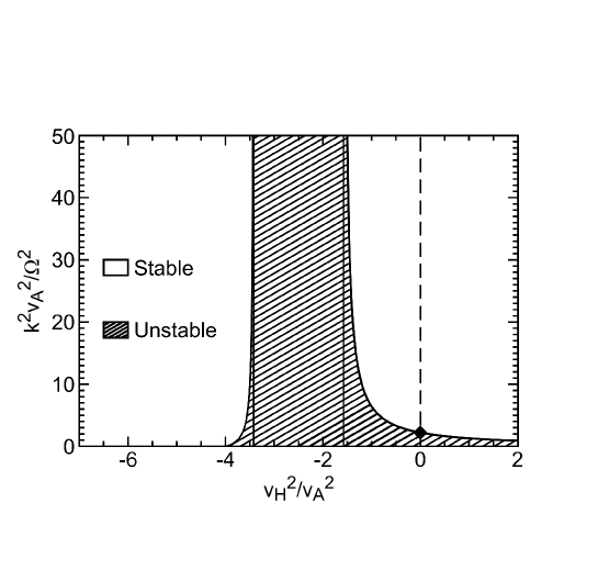
Figure 4: Range of unstable wavenumbers for a representative disk in the Hall-Ohm regime. The black diamond corresponds to the MRI without the Hall effect. The resistivity is chosen to be $\kappa^{2}\eta^{2}/v_{A}^{4}=0.35$. From Balbus & Terquem (2001).

6.3 Numerical Simulations of the Hall–Ohm–MRI.

What does the preceding section imply for the MHD transport properties of protostellar disks? The first local simulatons of the nonlinear development of the MRI in the presence of Ohmic resistivity are those of Fleming, Stone, & Hawley (2000). These authors found the important result that the nonlinear turbulent state is easier to maintain when a mean vertical magnetic field is present. This is sometimes misunderstood as a requirement that a disk must have a global vertical magnetic field to maintain MRI turbulence, but in fact all that the very local calculations of Fleming et al. (2000) really tell us is that on this scale, working with a precisely zero mean field is probably too restrictive an approximation for a real disk. This study found a difference of two orders of magnitude in the critical magnetic Reynolds number (defined here as the product of the isothermal times the box size divided by the resistivity) needed to sustain turbulence, depending upon whether a vertical field was present or not, the vertical field runs being the easier to sustain. It is now understood that very high resolution grids are needed for the local study of the MRI in a shearing box with zero mean field, so these early results should not be used quantitatively. With this precaution understood, it is interesting to note that for the vertical field runs, the Fleming et al. finding seems to be not very different from the ${\mathbb{L}}=1$ criterion discussed earlier.

This nature of the nonlinear behavior of a Hall fluid was examined in a numerical investigation by Sano & Stone (2002a,b). These authors carried out an extensive study of the local properties of Hall-MRI turbulence in the shearing box formalism. The results are somewhat surprising.

In linear theory, counteraligned magnetic and rotation axes produce a very broad wavenumber spectrum of instability, and should be more unstable than the aligned case. What Sano and Stone found, however, was just the opposite: the aligned case showed greater levels of field coherence and higher rms fluctuations than the counteraligned case. The reason for this is interesting, and illustrative of the hazards of extrapolating directly from linear theory.

In the case of counteraligned axes, the extended wavenumber of spectrum of linear MRI instability results, in its nonlinear resolution, in a highly efficient turbulent cascade to smaller and smaller scales. In a finite difference numerical simulation, this cascade terminates at the grid scale where energy is ultimately lost. By contrast, the aligned case shows instability only at longer wavelengths (small wavenumbers). At larger wavenumbers, the response of the fluid is wavelike, and this is likely to make a local small scale turbulent cascade considerably less efficient. The result: a less lossy system and greater large scale field coherence.

Finally, when simulations were done with half the field aligned with the rotation axis and half counteraligned, the Hall effect tended to wash out, and the results were similar to resistive MHD turbulence without the additional electromotive forces. The criterion for the onset of turbulence depended only the relative strength of the resistivity, as measured by the dimensionless number ${v_{A}^{2}/\eta\Omega}$. This so-called Lundquist number must be greater than unity or MRI-induced turbulence is not maintained, whether Hall electromotive forces are present or not, according to Sano & Stone. The presence of the Hall terms in the induction equation do, however, promote a slightly elevated rms level when turbulence can be maintained.

The Hall numerical studies are fascinating and suggestive, but caution is necessary before taking the final leap from simulation to real disks. Note, for example, the role played by the numerical grid scale losses in our discussion of the nonlinear resolution of the counteraligned case. Nature works without a grid, however, and it is not clear what scale ultimately intervenes at high wavenumbers in Hall protostellar disks. Moreover, it is now understood that there are important resolution questions for local shearing box simulations with no mean field, that have only recently been brought to light (Fromang et al. 2007; Lesur & Longaretti 2007). The important pioneering studies of Sano & Stone (2002a,b) merit a thoroughgoing follow-up on the much larger numerical grids that are currently available to numericists.

7 Alpha models of protostellar disks

7.1 Basic principles

We are now in a position to assemble a basic “$\alpha$ model” of a protostellar disk. An important assumption in such models is that angular momentum and mechanical energy are transported radially through the disk. We therefore work with height and azimuthally integrated quantities. Under these conditions, Balbus & Papaloizou (1999) have shown how the fundamental equations of MHD lead directly to the $\alpha$ formalism.

The velocities consist of a mean part plus a fluctuation of zero mean. For the azimuthal velocity $v\Phi$, the mean will be taken to be the Keplerian velocity

$$(R\Omega)^{2}={GM\over R}$$ (151)

where $M$ is the central mass and $G$ is the Newtonian constant. For the radial velocity $v_{R}$, the mean motion corresponds to the very slow inward accretion drift, $v_{2}$. The azimuthal fluctuation velocity $u_{\phi}$ is much less than $R\Omega$, whereas the radial fluctuation velocity $u_{R}$ is much larger than the inward drift. These claims will shortly be quantified. The magnetic field Alfvén velocities are assumed to be of the same order as the $u$ velocities, namely less than or of order the isothermal thermal sound speed $c_{S}$. To summarize,

$$v_{2}\ll u,v_{A},c_{S}\ll R\Omega.$$ (152)

Under steady-state conditions, the local disk accretion rate has a time averaged value of

$$\mu\equiv 2\pi R\langle\rho v_{2}+\delta\rho\,\delta u_{R}\rangle$$ (153)

The height integrated form of this is $-\dot{M}$, the mass accretion rate:

$$\int\mu\,dz=-\dot{M},$$ (154)

defined so that $\dot{M}$ is a positive constant. A useful average of $v_{2}$ is the drift velocity defined by

$$v_{d}\equiv-{\dot{M}\over 2\pi R\Sigma}$$ (155)

where $\Sigma$ is the disk surface density.

In steady-state, the height-integrated average radial angular momentum flux is proportional to $1/R$. In other words,

$$-\dot{M}R^{2}\Omega+2\pi\Sigma RW_{R\phi}=C/R$$ (156)

where $W_{R\Phi}$ is defined by

$$\int\langle\rho u_{R}u_{\phi}-\rho v_{AR}v_{A\phi}\rangle\,dz=\Sigma W_{R\phi},$$ (157)

and $C$ is a constant to be determined. Traditionally, this has been done by asserting that $W_{R\phi}$ is proportional to the radial gradient of $\Omega$, and at some point before the surface of the star is reached this must vanish. $C$ is then determined at this point (Pringle 1981).

This approach now seems dated, and especially inappropriate for a protostellar disk in which the magnetic interactions between the disk and star may become quite complex at small radii. Instead, let us note that at small $R$, $C/R$ must be very small if $\Sigma W_{R\phi}$ does not blow up, which seems quite reasonable. If $C/R$ is very small at the inner edge of the disk, it is clearly negligible in the body of the disk, and we shall set $C=0$ with the understanding that our solution should not be taken to the stellar surface. Then, (156) reduces to

$$v_{d}=-{W_{R\phi}/R\Omega}$$ (158)

showing that $v_{d}$ (and $v_{2}$ which is of the same order) is very small compared with the $u$ velocities. Alternatively,

$$\Sigma W_{R\phi}={\dot{M}}R\Omega/2\pi.$$ (159)

This is a particularly useful result because $W_{R\phi}$ appears in the energy balance equation (140):

$$-\Sigma W_{R\phi}{d\Omega\over d\ln R}=-{d\Omega\over d\ln R}\int T_{R\phi}\,dz=\int\rho{\cal L}\,dz=2\sigma T_{eff}^{4}.$$ (160)

In the last equality, we have equated the radiated energy per unit surface of the disk to twice the blackbody emissivity, the factor of two represents two radiating surfaces. Here $\sigma$ is the Stefan-Boltzmann constant and $T_{eff}$ is the effective blackbody surface temperature. Combining (159) and (160) then gives us

$$T_{eff}^{4}={3GM\dot{M}\over 8\sigma\pi R^{3}},$$ (161)

relating the potentially observable disk surface temperature to the central mass, accretion rate, and radial location. The unknown turbulent stress parameter $W_{R\phi}$ has conveniently vanished!

Equation (161) is in a restricted sense “exact.” It is based on the assumption of time-steady conditions and thermal radiation, but it is independent of the explicit nature of the turbulence, as long as it is local. If these conditions are all met, equation (161) is a simple matter of energy conservation. To go beyond this result, something has to be said directly about $W_{R\phi}$. In $\alpha$ disk theory, that condition is

$$W_{R\phi}=\alpha c_{S}^{2}$$ (162)

where $\alpha$ is assumed to be constant, but otherwise unknown. In contrast to the simple and plausible assumption that turbulence is locally dissipated, this “$\alpha$ assumption” is far from obvious, and in a strict mathematical sense almost certainly wrong.

The original justification for this form of the stress tensor was based on the notion of hydrodynamical turbulence and the idea that the velocity fluctuations would be restricted to some fraction of the sound speed (fluctuations in excess would cause shocks). Shakura & Sunyaev (1973) consider magnetic stresses, however, and argue that they fit within the $\alpha$ formalism as well since Alfvén velocities in excess of $c_{S}$ are also dynamically unlikely.

The real problem with the prescription (162) is that turbulence is just too complicated. Not only are long term averages very hard to define (a problem even for a result like equation [161]), it is also entirely possible that $\alpha$ could vary in a complex nonsystematic way by an order of magnitude or more from one part of the disk to another. The primary justification for (161) is that many scaling results are very insensitive to $\alpha$. On dimensional grounds $c_{S}$ is is certainly an important local characteristic velocity, but it is not yet clear under what conditions a “background” magnetic field might also be providing a mean Alfvén velocity that limits or guides the turbulence.

Continuing with our $\alpha$ model, to link the surface temperature $T_{eff}$ with the midplane temperature $T$ (used in quantities like $c_{S}$) we need to introduce explicit vertical structure into the problem. The hydrostatic equilibrium equation is

$$-{\partial P\over\partial z}={GM\rho z\over R^{3}}=\rho z\Omega^{2}$$ (163)

This may be solved in conjunction with a detailed energy equation, but it seems best for illustrative purposes to note that this equation serves to provide a decent and very simple estimate of the disk half thickness, $H=c_{S}/\Omega$. The energy equation for simple vertical radiative diffusion defines the local radiative energy flux $F_{\gamma}$ as:

$$F_{\gamma}={4\sigma\over 3}{dT^{4}\over d\tau}.$$ (164)

The “optical depth” $\tau$ is given by

$$d\tau=-\rho\kappa dz$$ (165)

where $\kappa$ is the opacity of the disk (units: cross sectional area per unit mass). In the simplest possible model, $F_{\gamma}$ is a constant given by $\sigma T_{eff}^{4}$, and the temperature at the midplane $T$ is then

$$T^{4}={3\tau T_{eff}^{4}\over 4}$$ (166)

where $\tau$ is the optical depth from the outer disk surface to the midplane. (In this simplest of all possible models, we set $\tau=\kappa H$, where $\kappa$ is evaluated at the midplane temperature.)

The surface temperature of a disk with a mass accretion rate of $10^{-8}M_{\odot}$ per year around a $1M_{\odot}$ star is $85R_{AU}^{-0.75}$K, where $R_{AU}$ is the radius in astronomical unit. The midplane temperature $T$ is a factor $\sim\tau^{1/4}$, larger, typically a factor of 5 or so larger. At what value of $T$ would we expect the ionization fraction to reach the critical value of $10^{-13}$ we found earlier, corresponding to a Lundquist number of unity? Put in somewhat different terms, is our model of self-sustaining MHD turbulence self-consistent?

To answer this, we need to address the physics of thermal ionization. In the low ionization regime we are working, thermal electrons are supplied by trace alkali elements, notably potassium, with an ionization potential of only 4.341 eV. Even this modest value corresponds to an effective temperature of 50,375 K, well above the range of $10^{2}$ to $10^{3}$K we expects, and potassium will barely be ionized.

The equation governing the ionization fraction $x$ is the Saha equation. In this barely ionized regime, it may be written (Stone et al. 2000)

$$x^{2}=as\left(2.4\times 10^{15}\over n\right)T^{3/2}\exp(-50375/T)$$ (167)

where $a$ is the abundance of potassium ($~{}10^{-7}$), $n$ is the ratio of the dominant $H_{2}$ molecules, and $s$ is a ratio of statistical weights, expected to be near unity. We may rewrite this equation as

$$T=-{50375\over\ln X}$$ (168)

where

$$X=x^{2}T^{-3/2}(n/2.4\times 10^{15})$$ (169)

With $x=10^{-13}$ and the final density factor anything between 0.01 and 1 ($0.1M_{\odot}$ of gas spread out over a region of 10 AU yields a density of about $5\times 10^{13}$ per cc) gives values for $T$ close to $10^{3}$K, which we will adopt as a working number.

Therefore, a surface temperature of about $200$K is required to attain a midplane temperature of $10^{3}$, and thereby ensure a critical level of ionization. This is the key issue for MHD theories of protostellar disks: beyond $0.2-0.3$AU, or $\sim 3\times 10^{12}$cm, the heat generated by the dissipation associated with local turbulence is insufficient to keep the the disk magnetically well-coupled. Where and how do protostellar disks maintain good magnetic coupling?

8 Ionization Models of Protostellar Disks

8.1 Layered accretion

The above considerations indicate that dissipative heating from MHD turbulence self-consistently generates enough heat to maintain the minimum thermal levels of requisite ionization only with a few 0.1 AU. Nonthermal sources of ionization are therefore of great interest to protostellar disk theorists. The principle ionizing agents that have been studied are cosmic rays, X-rays, and radioactivity.

Gammie (1996) argued that the low density extended vertical layers of a protostellar disk would be exposed to an ionizing flux of interstellar cosmic rays. Just as in models of molecular cloud ionization, cosmic rays would maintain a minimal level of ionization in the upper disk layers. The range of the low energy galactic cosmic rays is about 100 g/cm². This is much less than the disk column density at $\sim 1$ AU in generic solar nebula models, but can easily exceed the disk column at larger distances. If the level of ionization is high enough–and the Alfvén velocity $v_{A}$ is small enough—the gas within the range of the cosmic rays will be MRI active. (The Alfvén velocity cannot be too large if disturbances are not to be stablized by magnetic tension.) If these criteria are met, Gammie argued that turbulent accretion would proceed in the outer layers of protostellar disks, but that the midplane regions would remain laminar—in effect, a “dead zone.” This is the basis of the concept of layered accretion, which has become an important idea in protostellar disk modeling (Sano et al. 2000).

Gammie’s original construction was based on the assumptions that the accretion would occur in a layer of fixed column, and that $\alpha$ is constant. Taken together, these assumptions preclude a steady solution; the mass flux rate is not independent of position. Instead, matter is deposited from the outer regions into the disk’s inner regions where it builds up. At some point in this scenario the disk become gravitationally unstable, and it was speculated that an accretion outburst might occur, which was tenatively identified with FU Orionis behavior. On the other hand, there is no compelling argument (beyond mathematical convenience) to prevent the $\alpha$ parameter from adjusting with position, if this allows a relaxation to a time steady solution. The overarching layered accretion picture would, however, remain intact with this modification.

YSO’s are almost universally X-ray sources. Glassgold et al. (2000) noted that X-rays are potentially a far more powerful ionization source, even if attenuated, than galactic cosmic rays. These authors were thus the first to draw the link between X-ray observations and MRI activity of accretion disks. In the Glassgold et al. formulation, X-rays from a locally extended corona centered on the YSO irradiate the disk, and depending upon the chosen parameters, could provide the requisite ionization levels to lessen the extent of the dead zone or eliminate it altogether.

Whether the dead zone persists in the presence of X-ray irradiation or not depends, among other things, upon the model adopted for the disk structure. Generally, the so-called minimum mass solar nebula model (Weidenschilling 1977) is used. This is a reconstruction of the surface density distribution of the sun’s protostellar disk based on current planetary masses and compositions, and results in an $R^{-3/2}$ radial distribution. Fromang, Terquem, & Balbus (2002) suggested that ionization fractions should be calculated self-consistently within the framework of accretion disk theory, which in general leads to a more shallow dependence of surface density with radius. By introducing accretion parameters whose values are free ($\alpha$ and the mass accretion rate $\dot{M}$), the range of parameter space increases, and the presence and extent of a dead zone becomes yet more model dependent.

The ionization fraction of a protostellar disk is a chemical problem, and in principle can involve a very complex, uncertain, molecular reaction network. Ilgner & Nelson (2004a) investigated the consequences for the dead zone of a considerably richer chemical network. While the quantitative details were sensitive to the chemistry, the qualitative structure was not. A dead zone is likely to be present in any plausible chemical network that has been studied up to the present, but there are conditions in which its extent can be very small or possibly even zero. Ilgner & Nelson (2004b), for example, made the interesting comment that flaring activity by the central star can have a significant effect on the extent of the dead zone.

8.2 Activity in the Dead Zone

Just because the dead zone is unable to host the MRI does not mean that it is well and truly dead. Fleming and Stone (2003) carried out numerical simulations in which the magnetically active upper layers of the disk coupled dynamically to the magnetically inert dead zone, resulting in a small but significant Reynolds stress, even though the Maxwell stress was zero. More recently, Turner & Sano (2008) suggested that the high resistivity characteristic of the dead zone is also a means for magnetic field to diffuse into this region from the active layers. Moreover, these authors point out, an active MRI region is not an absolute prerequisite for accretion: direct magnetic torques on much larger scales would also serve, and since they do not dissipate energy in a turbulent cascade, are much less costly to maintain.

Terquem (2008) constructed global models of protostellar disks based on the $\alpha$ prescription. The presence of a dead zone was surprisingly nondisruptive, provided that $\alpha$ was not too small. Steady solutions were found for values of $\alpha$ in the dead zone as small as $10^{-3}$ times the active zone value. In these models, the dead zone was thicker and more massive than its surroundings, but because of the relatively weak $\alpha$ scalings, by less than an order of magnitude. These results, taken as a whole, suggest that an embedded dead zone in a protostellar disk is not necessarily disruptive to the accretion process.

8.3 Dust

In all of our discussions, we have been most negligent by not mentioning the effects of small dust grains (e.g. Sano et al. 2000). Let us see crudely why this is so.

Consider a mass $M$ of protostellar disk gas, of which $10^{-2}M$ is in the form of spherical dust grains of radius $r_{d}$. If the dust grains have a density of 3 gm cm^-3, there are a total of

$$N_{d}=(10^{-2}/4\pi)(M/r_{d}^{3})$$

grains in a volume $V$. The grains present a geometric cross section of $\sigma_{d}=\pi r_{d}^{2}$ (we ignore here the enhancement due to the induced charge [Drain & Sutin 1987]), and the electrons have an average radial velocity of some $v_{e}=1.6(kT/m_{e})^{1/2}$. The total dust recombination rate per unit volume is

$$(N_{d}/V)n_{e}\sigma_{d}v_{e}$$ (170)

where $n_{e}$ is the number density of electrons. This should be compared with a typical dielectronic recombination rate of $\beta\equiv 8.7\times 10^{-6}$ cm³ s^-1(Glassgold, Lucas, & Omont 1986; Gammie 1996). If $x$ is ionization fraction, then the ratio of dielectronic recombination to dust recombination is

$${n_{e}\beta V\over N_{d}\sigma_{d}v_{e}}\sim\left(x\over 10^{-13}\right){r_{d}\over T}$$ (171)

where $r_{d}$ is in cm and $T$ in K. For small dust grains ($\sim 10^{-5}$cm) this ratio is $\ll 1$ and dust recombination is overwhelmingly important. But the relative importance of the grains diminishes as they grow in size, especially in the cooler portions of the disk. Sano et al. (2000) concluded that in their model (based on cosmic ray ionization) a typical protostellar disk would be MRI stable inside of about 20 AU if small grain are present, except for the innermost regions which would be thermally ionized.

The detailed effects of dust grains have been considered by many authors; a very good review and list of references is given in the recent paper of Salmeron & Wardle (2008). These authors have considered the vertical structure of the magnetic coupling in a minimum mass solar nebula model, including the effects of Hall electromotive fores and ambipolar diffusion. They employed a sophisticated chemical network (Nishi et al. 1991), and small dust grains ranging in radius from 0.1 to 3 microns. At the fiducial locations of 5 and 10 AU, Salmeron & Wardle found good magnetic coupling over an impressive range of magnetic field strengths provided for the 3 micron grains, a considerable imporovement from our naive estimate above. For the 0.1 micron grains, the magnetic coupling dropped sharply (as did MRI growth rates), and was restricted to higher elevations above the disk plane.

9 Summary

Protostellar disks are gaseous systems dynamically dominated by Keplerian rotation. These disks are accreting onto the central protostar, so there must be a source of enhanced angular momentum transport present. In the early stages of the disk’s life, this enhanced transport may well be due to self-gravity, with density waves largely responsible for moving angular momentum outwards. Once the disk becomes observable, its mass is below the minimum needed to sustain self-gravitational spiral wave transport. The only established mechanism able to sustain high levels of angular momentum transport is MHD turbulence produced by the magnetorotational instability, or MRI.

The dynamical effects of magnetic fields on protostellar disks depends crucially on the degree of ionization, more specifically on the electron fraction, that is present. This means that there is a direct link between the gross dynamical behavior of a protostellar disk and its detailed chemical profile. In principle, the full multifluid nature of the disk gas — neutrals, ions, electrons, and dust grains — must be grappled with at some level to elicit and understand the disk strucutre. Fortunately, only a very small ionization level is needed to couple the charged and neutral components, leaving (in essence), a single magnetized fluid. An electron fraction of $10^{-13}$ is a typical fiducial number for the threshold of magnetic coupling at 1 AU in the T Tauri phase of the solar nebula: roughly one electron per cubic millimeter of disk gas! Unfortunately, however, on scales of 10’s of AU, near the dense midplane the ionization of protostellar disks may not even rise to this minimal level of ionization. At the boundary between good and poor magnetic coupling, the MHD processes are complex, not well-understood, and the domain of ongoing inquiry.

In regions of the disk where the magnetic coupling is sufficient, the combination of a weak (subthermal) magnetic field and Keplerian rotation leads to the MRI. In ideal MHD, the magnetic field behaves as though it were frozen into the conducting gas, and the presence of differential rotation produces azimuthal magnetic field from a radial magnetic field. But this is not all that happens. If one tries to simulate this simple process on a computer, the laminar flow breaks down into a turbulent mess, even if the field is very weak.

The reason for this is due to another classical property of magnetic fields, that the force exerted by the lines of force on the background gaseous fluid is the sum of a pressure-like term and a tension-like term. It is the latter tension-like term that is important for an understanding of the MRI. When two nearby fluid elements are moved apart, even if only because of a random perturbation, the magnetic tension force acts precisely like a spring coupling the two masses. The fluid element on the inside rotates faster than the element on the outside, and tries to speed it up. The outer element, in acquiring angular momentum from the inner element, finds itself too well-endowed, and spirals outward toward a higher orbit where its excess angular momentum can be accommodated. On the other hand, the inner element, having lost angular momentum, finds itself at a deficit and must drop to a lower angular momentum orbit. This separation stretches the field lines that couple the elements, the magnetic tension goes up, and the process runs away. This is the MRI. Notice that angular momentum transport is at the very core of the linear instability, rather than the result of some sort of nonlinear mixing process.

But the MRI does, in fact, lead to rapid turbulent mixing of the disk gas, as outwardly moving and inwardly moving fluid elements encounter one another and dissipate their energy. If this happens locally, then the ingredients for a classical $\alpha$ model of accretion are present. To the extent that many disk features are insensitive to, or independent of, the precise rms level of the disk fluctuations, these models can be of some practical utility. The classical formula relating the disk emissivity to radius $R$ is the most important instance of this.

In real protostellar disks, the level of ionization present is such that there are significant departures from the behavior of an ideal (perfectly conducting) MHD gas. In principle, the gas can become completely decoupled from the magnetic field, and go over to a hydrodynamic system. Less dramatically, the current-bearing electrons can acquire a velocity significantly different from the dominant neutrals, since the former need to maintain a current density and magnetic field even as charged species become rarer and rarer. When this happens, the field lines are no longer frozen into the motion of the bulk of the (neutral) disk gas, they are frozen into the electrons and the distinction becomes important. In the so-called Hall regime, the ions and neutrals move together distinctly from the electrons, and the ion motion relative to the electron-following field lines induces an additional electromotive force into the gas, beyond the self-induction responsible for simple field line freezing. Hall MHD is likely to be important in protostellar disks on scales of AU to 10’s of AU scales.

Dust grains are an ever present complication for MHD disk modeling. Typically, solids make up about 1 percent of the mass of interstellar gas. An interstellar population of small grains (radius $\sim 10^{-5}$ cm) with a total mass fraction of a percent would present an enormous collecting area of would-be gas phase electrons. Putting charges on the grains effectively removes them because of the low mobility of the grains. Determining the disposition of the dust grains is thus a necessity for constructing MHD disk models. As the disk evolves, so too do the dust grains. They grow in size as they agglomerate, and they tend to settle towards the midplane, if they are not stirred by turbulence or some other dynamical process. Larger dust grains are much less efficient in removing gas phase electrons than are smaller grains, where “larger” means growth in radius of an order of magnitude or more.

Where does all of this leave us? Clearly, we are a long way from framing a picture of protostellar disk evolution at the level of, say, classical stellar evolution. But for all of the gaping uncertainties, a useful zeroth order MHD-based picture of a protostellar disk in its T Tauri phase can be cobbled together:

Inside of about $0.3$ AU, a protostellar disk will be thermally ionized by direct exposure to the central source and self-consistently by the dissipation of MHD turbulence. We may expect vigorous MRI induced MHD turbulence in this zone.

On scales of AU’s, thermal ionization is no longer adequate to maintain the requiste levels of ionization to ensure MHD coupling, at least not near the high density midplane. Depending upon the X-ray luminosity of the central star, the spectrum of dust grains and the abundance of gas phase potassium and sodium (electron donors), there could be good coupling at low density, higher elevation disk altitudes. The “dead zone” at lower altitudes need not be devoid of all transport; density waves from an adjacent active layer or large scale magnetic torques would each contribute their own stresses. It is even possible that some degree of coupling could be maintained down to the disk midplane, though this depends strongly on modeling assumptions. It seems likely, however, that on a scale an AU to tens of AU’s , the level of MHD turbulence will be far less than in the disk’s innermost regions.

Finally, on scales larger than tens of AU’s, the falling density lengthens recombination times and suggests a return to good MHD coupling. The typical size of a disk is many hundred AU’s so that the dead zone is small when viewed globally, and may not have much of an impact in the overall accretion process (Terquem 2008). Perhaps, however, it is not coincidence that the MHD “quiet zone” coincides with the region of planet formation in the solar nebula and (more speculatively) in other protostellar disks.

Appendix A

Begin with equation (16):

$${\mbox{\boldmath{$J$}}\over c}\mbox{\boldmath{$\times$}}\mbox{\boldmath{$B$}}=\mbox{\boldmath{$p_{In}$}}+\mbox{\boldmath{$p_{en}$}}$$ (172)

where the right side of this equation is

$$n_{I}n\mu_{In}\langle\sigma_{nI}w_{nI}\rangle(\mbox{\boldmath{$v_{I}$}}-\mbox{\boldmath{$v$}})+n_{e}nm_{e}\langle\sigma_{ne}w_{ne}\rangle[(\mbox{\boldmath{$v_{e}$}}-\mbox{\boldmath{$v_{I}$}})+(\mbox{\boldmath{$v_{I}$}}-\mbox{\boldmath{$v$}})]$$ (173)

In what follows, we will often need an estimate of the ratio of the ion and electron collision rates. Following our discussion in section 3, we will assume that

$${\langle\sigma_{nI}w_{nI}\rangle\over\langle\sigma_{ne}w_{ne}\rangle}=\left({m_{e}\over\epsilon\mu_{In}}\right)^{1/2}$$ (174)

where $\epsilon<1$ is inserted because the electron-neutral cross section is geometrical, while the ion-neutral collision cross section is larger than geometrical.

In (173), the first $(\mbox{\boldmath{$v_{I}$}}-\mbox{\boldmath{$v$}})$ term dominates the last by a factor of order $(\mu_{In}/\epsilon m_{e})^{1/2}$. Hence,

$$\mbox{\boldmath{$p_{In}$}}={\mbox{\boldmath{$J$}}\over c}\mbox{\boldmath{$\times$}}\mbox{\boldmath{$B$}}-\mbox{\boldmath{$p_{en}$}}={\mbox{\boldmath{$J$}}\over c}\mbox{\boldmath{$\times$}}\mbox{\boldmath{$B$}}+{nm_{e}\over e}\langle\sigma_{ne}w_{ne}\rangle\mbox{\boldmath{$J$}}$$ (175)

With the help of equation (10), this implies

$$\mbox{\boldmath{$v_{I}$}}-\mbox{\boldmath{$v$}}={\mbox{\boldmath{$J\times B$}}\over c\gamma\rho\rho_{I}}+\underbrace{\sqrt{\epsilon m_{e}\over\mu_{nI}}Z(\mbox{\boldmath{$v_{I}$}}-\mbox{\boldmath{$v_{e}$}})}_{A}.$$ (176)

We have marked the term with an “A” for future reference.

Recall equation (20):

$$\mbox{\boldmath{$E$}}+{1\over c}\left[\mbox{\boldmath{$v$}}+(\mbox{\boldmath{$v_{e}$}}-\mbox{\boldmath{$v_{I}$}})+(\mbox{\boldmath{$v_{I}$}}-\mbox{\boldmath{$v$}})\right]\mbox{\boldmath{$\times$}}\mbox{\boldmath{$B$}}+{m_{e}\nu_{en}\over e}\left[(\mbox{\boldmath{$v_{e}$}}-\mbox{\boldmath{$v_{I}$}})+(\mbox{\boldmath{$v_{I}$}}-\mbox{\boldmath{$v$}})\right]=0.$$ (177)

In substituting equation(176) for $\mbox{\boldmath{$v_{I}$}}-\mbox{\boldmath{$v$}}$ in the above, we may always drop the “A” term, since it is small compared with $\mbox{\boldmath{$v_{e}$}}-\mbox{\boldmath{$v_{I}$}}$.

Proceeding with the above substitution leads to

$$\mbox{\boldmath{$E$}}+{\mbox{\boldmath{$v$}}\over c}\mbox{\boldmath{$\times$}}{B}-{\mbox{\boldmath{$J\times B$}}\over en_{e}c}\bigg{[}1-\underbrace{{m_{e}\nu_{en}n_{e}\over\gamma\rho\rho_{I}}}_{B}\bigg{]}+{(\mbox{\boldmath{$J\times B$}})\mbox{\boldmath{$\times$}}\mbox{\boldmath{$B$}}\over c^{2}\gamma\rho\rho_{I}}-{\mbox{\boldmath{$J$}}\over\sigma_{cond}}=0,$$ (178)

where $\sigma_{cond}$ is defined in equation (24). The “B” term in the above equation may now clearly be dropped: it is of order $Z(\epsilon m_{e}\mu_{nI})^{1/2}/m_{n}$. This leads to

$$\mbox{\boldmath{$E$}}+{\mbox{\boldmath{$v$}}\over c}\mbox{\boldmath{$\times$}}{B}-{\mbox{\boldmath{$J\times B$}}\over en_{e}c}+{(\mbox{\boldmath{$J\times B$}})\mbox{\boldmath{$\times$}}\mbox{\boldmath{$B$}}\over c^{2}\gamma\rho\rho_{I}}-{\mbox{\boldmath{$J$}}\over\sigma_{cond}}=0,$$ (179)

which is precisely equation (23) in the text.

Appendix B:

To estimate the order of departures from charge neutrality or the displacement currents, we will assume that the $\nabla$ operator is $\sim 1/L$, where $L$ is a characteristic length scale of the flow, and $\partial/\partial t$ is $\sim v/L$, where $v$ is a characteristic velocity (say, the largest of the neutral, ion, or electron velocities).

For the electric field, we take $E\sim vB/c$, since we are only interested in problems where the inductive terms are comparable to, or in larger than, the resistive damping. Then

$$\mbox{\boldmath{$\nabla$}}\mbox{\boldmath{$\cdot$}}\mbox{\boldmath{$E$}}\sim E/L\sim vB/Lc\sim 4\pi vJ/c^{2}\sim 4\pi en_{e}v^{2}/c^{2}$$ (180)

Hence, the divergence of $E$ is of order $v^{2}/c^{2}$ times the electron charge density (at most, since we assumed $v_{I}-v_{e}\sim v$ in the above). It may thus be ignored.

For the displacement current, the demonstration is almost a matter of direct inspection. If we take the curl of equation (29) and use equation (27), then the on the right side of (29) the first term is $\sim B/L^{2}$, while the second, displacement, term is $\sim v^{2}B/c^{2}$. It may thus be ignored.

References

- (1) Balbus, S. A. 2001, ApJ, 562, 909
- (2) Balbus, S. A. 2003, ARAA, 41, 555
- (3) Balbus, S. A., & Hawley, J. F. 1991, ApJ, 376, 214
- (4) Balbus, S. A., & Hawley, J. F. 1992, ApJ, 392, 662
- (5) Balbus, S. A., & Hawley, J. F. 1998, Rev. Mod. Phys., 70, 1
- (6) Balbus, S. A., & Hawley, J. F. 2000, in From Dust to Terrestrial Planets, eds. W. Benz, R. Kallenbach, G. Lugmaier, and F. Podosek, ISSI Space Sciences Series No. 9, Space Science Reviews, 92, 39
- (7) Balbus, S. A., & Papaloizou, J. C. B. 1999, ApJ, 521, 650
- (8) Balbus, S. A., & Terquem, C. 2001, ApJ, 552, 235
- (9) Blaes, O. M., & Balbus, S. A. 1994, ApJ, 421, 163
- (10) Draine, B. T., Roberge, W. G., & Dalgarno A. 1983, ApJ, 264, 485
- (11) Draine, B. T., & Sutin, B. 1987, ApJ, 320, 803
- (12) Fleming, T., & Stone J. M. 2003, ApJ, 585, 908
- (13) Fleming, T., & Stone J. M., & Hawley, J. F. 2000, ApJ, 530, 464
- (14) Fromang, S., Terquem C., & Balbus, S. A. 2002, MNRAS, 329, 18
- (15) Fromang, S., Papaloizou, J., Lesur, G., & Heinemann, T. 2007, A&A, 476, 1123
- (16) Gammie, C. F. 1996, ApJ, 457, 355
- (17) Glassgold, A. E., Feigelson, E. D., Montmerle, T. 2000, in Protostars and Planets IV, V. Mannings, A. P. Boss, S. Russel eds. (U. Arizona Press: Tucson), 429
- (18) Glassgold, A. E., Krstic̀, P. S., & Schultz, D. R. 2005, ApJ, 621, 808
- (19) Glassgold, A. E., Lucas, R., & Omont, A. 1986, AA, 157, 35
- (20) Hartmann, L. 1998, Accretion Processes in Star Formation (Cambridge: Cambridge University Press)
- (21) Ilgner, M., & Nelson, R. P. 2004a, AA, 445, 205
- (22) Ilgner, M., & Nelson, R. P. 2004b, AA, 455, 731
- (23) Jackson, J. D. 1975, Classical Electrodynamics (2nd. ed.) (Wiley: New York)
- (24) Ji, H., Burin, M., Schartman, E., & Goodman, J. 2006, Nature 444, 343
- (25) Kunz, M. W., & Balbus S. A. 2004, MNRAS, 348, 355
- (26) Landau, L. D., & Lifshitz, E. M. 1959, Fluid Mechanics (London: Pergamon Press)
- (27) Lesur, G., & Longaretti, P.-Y. 2007, MNRAS, 378, 1471
- (28) Lin, D. N. C., & Papaloizou, J. 1980, MNRAS, 191, 37
- (29) Lin, D. N. C., & Papaloizou, J. C. B. 1996, ARAA, 34, 703
- (30) Lubow, S. H., Papaloizou, J. C. B., & Pringle, J. E. 1994, MNRAS, 267, 235
- (31) Moffatt, H. K., Kida, S., & Ohkitani K. 1994, J. Fluid Mech., 259, 241
- (32) Nishi, R., Nakano, T., Umebayashi, T. 1991, ApJ, 368, 181
- (33) Papaloizou, J. C. B., & Lin, D. N. C. 1995, ARAA, 33, 505
- (34) Pneuman, G. W., & Mitchell, T. P. 1965, Icarus, 4, 494
- (35) Pringle, J. E, 1981, ARAA, 19, 137
- (36) Reipurth, B., Jewitt, D., & Keil, K. (eds.) 2007, Protostars and Planets V, (U. Arizona Press: Tucson)
- (37) Richard, D. 2001, Ph. D. Thesis, Univ. Paris 7
- (38) Sano, T., Miyama, S. M., Umebayashi, T., & Nakano, T. 2000, ApJ, 543, 486
- (39) Sano, T., & Stone, J. M. 2002a, ApJ, 570, 314
- (40) Sano, T., & Stone, J. M. 2002b, ApJ, 577, 534
- (41) Salmeron, R., & Wardle M. 2008, MNRAS 388, 1223
- (42) Shakura, N. I., & Sunyaev R. A. 1973, AA, 24, 337
- (43) Stone, J. M., & Balbus, S. A. 1996, ApJ, 464, 364
- (44) Stone, J. M., Gammie, C. F., Balbus, S. A., & Hawley, J. F. 2000, in Protostars and Planets IV, eds. V. Mannings, A. Boss, and S. Russell, Space Science Reviews, (U. Arizona Press: Tucson), 589
- (45) Terquem, C. 2008, ApJ, in press.
- (46) Turner, N. J., & Sano, T. 2008, ApJ, 679L, 131
- (47) Velikhov, E. P. 1959, Sov. Phys. JETP, 36, 995
- (48) Wardle, M. 1999, MNRAS, 307, 849
- (49) Weidenschilling, S. J. 1977, Astrophys. & Space Science, 51, 153
- (50) Zel’dovich, Ya. B., Ruzmaikin, A. A., & Sokoloff, D. D. 1983, Magnetic Fields in Astrophysics (Gordon and Breach: New York)