Fluctuating solutions for the evolution of domain walls

Abstract

A class of oscillating Lorentz covariant configurations for the evolution of the domain walls in diverse dimensions are analytically obtained. It is shown that the oscillating solutions in the case of domain walls are responsible for structures which are larger than the usual kink-like configurations and, in the Lorentz covariant evolution case, lead to long-standing configurations.

1 Introduction

The study of nonlinear systems have been growing since the sixties of the last century [1, 2]. Nowadays the nonlinearity is found in many areas of the physics, including condensed matter physics, field theory, cosmology and others [3]-[24]. Particularly. whenever we have a potential with two or more degenerate minima, one can find different vacua at different portions of the space. Thus, one can find domain walls connecting such regions.

In a beautiful and seminal work, Coleman [25, 26] described what it was called the “fate of the false vacuum” through a semiclassical analysis of an asymmetric $\lambda\phi^{4}$-like model. In such situation the decaying process of the field configuration from the local to the global vacuum of the model is analyzed. In a very recent work by Dunne and Wang [27], it was shown that in the presence of gravity some fluctuating bounce solutions show up. In that work, those oscillating bounces where numerically obtained. Here we will show that those beautiful unusual field configurations appear already in the case where there are no gravitational interaction. Interestingly, in the work of Dunne and Wang, it has been asserted that those fluctuating solutions do not appear in the flat-space limit. However, in their work they analyzed the system through an Euclidean action. Here, instead, we work with a Minkowski space-time metric. Furthermore, they were concerned with instanton solutions ($\phi\left(t\right)$), and we deal with kinks and lumps ($\phi\left(x\right)$).

As observed by Coleman [25], this kind of system can be used to describe nucleation processes on statistical physics, crystallization of a supersaturated solution, the boiling of a superheated fluid and even in the case of the evolution of cosmological models.  In this last application, one can suppose that when the universe have been created it was far from any vacuum state. As it has expanded and cooled down it evolved first to a false vacuum instead of the true one. Thus, in such a scenario, when the time goes by, the universe should finally be settled in the true vacuum state. As we are going to see below, an evident and important consequence of the existence of these oscillating solutions is that the decaying process can be retarded when compared with the non-fluctuating configurations. Furthermore, if one takes into account the case of static domain walls, it is clear that the oscillating configurations are responsible for structures which are larger than the usual kink-like configurations. So one can use those solutions in order to describe thicker walls.

Besides, as we will see below, there are some covariant fluctuating configurations, which are capable to describe systems where the configuration evolves from the false to the true vacuum. The duration of the evolution from a vacuum to another, depends on the number of oscillations. As observed above, this can be used to describe some possible long-standing cosmological evolutions. Moreover, one can think also about ferromagnetic systems which, beginning with randomly distributed magnetic domains, are submitted to an external magnetic field. In this situation, the domains which present an orientation of their magnetization along the direction of the external field, can be thought as living in the true vacuum. The remaining will be in the false ones and, as a consequence, will tend to evolve to the true vacuum by aligning themselves with the external magnetic field. This process probably will not happens suddenly but, on the contrary, they might oscillate before reaching the true vacuum. This process would take a longer time to occur, when compared with a direct evolution from the false to the true vacuum, as we see below in this work.

Aiming to achieve those analytical solutions, we are concerned with a model which is a modification of the one introduced by Horovitz, following a suggestion of S. Aubry, when studying the presence of solitons in discrete chains, Horovitz and collaborators [28] introduced the so-called Double-Quadratic (DQ) [29]-[32] model, whose potential is given by

$$V(\phi)=\frac{1}{2}\phi^{2}-\left|\phi\right|+\frac{1}{2}.$$ (1)

That mentioned model was introduced by Stavros Theodorakis [31]. It allows one to obtain explicit analytical solutions for the kink-like and lump-like field configurations, these last were called in that paper as critical bubbles. The model introduced in [31] is an asymmetrical version of the DQ model (ADQ), and it is characterized by the potential

$$V(\phi)=\frac{1}{2}\phi^{2}-\left|\phi\right|-\epsilon\phi+\frac{1}{2}(\epsilon-1)^{2},$$ (2)

where $0<\epsilon<1$. In Fig. 1 this potential is plotted. In fact, a similar potential was used in order to analyze the case of wetting and oil-water-surfactant mixtures [33]. So, the solutions described here will may also have important impact over this matter.

It can be seen that it is a kind of asymmetrical $\lambda\phi^{4}$ model, where the potential has a derivative discontinuity at $\phi=0$, what was called a “kink” in [31], and this is in contrast with the usual meaning used for the word kink in the quantum field theory literature. Here we use this last nomenclature instead, where the word kink stands for a field configuration which interpolates between different vacua of the model, and lump corresponds to a configuration where the field interpolates a vacuum with itself. In the next sections, we will construct explicitly some examples of the new class above mentioned, and discuss the physical features of the analytical solutions. Finally, we will present a generalization for an arbitrary number of oscillations at the conclusions section. In particular, in Section 4, the extension of the evolution domain walls [31] is taken into account.

2 New kinks and lumps in one spatial dimension

In this section we present the first example of an entire new class of static lump and kink-like solutions for the ADQ model. For this, we suppose that there are four regions where the field presents alternating signals. Specifically, we look for a solution where $\phi_{I}<0$, $\phi_{II}>0$, $\phi_{III}<0$ and $\phi_{IV}>0$. As a consequence, the points, $x_{1}$, $x_{2}$ and $x_{3}$ which separate these regions, shall correspond to zeros of $\phi(x)$.

The finiteness of the solution along the whole spatial axis imply into a restriction of the integration constants. Additionally, we require that the field approaches asymptotically the vacua of the model, respectively given by $\phi_{I}(-\infty)=-1+\epsilon$ and $\phi_{IV}(\infty)=1+\epsilon$. Moreover, since the field must vanish at the intermediate points, we shall grant that $\phi_{I}(x_{1})=\phi_{II}(x_{1})=0$, $\phi_{II}(x_{2})=\phi_{III}(x_{2})=0$ e $\phi_{IV}(x_{3})=\phi_{IV}(x_{3})=0$. Thus, we finish with

$$\phi_{I}(x) = (1-\epsilon)(e^{x-x_{1}}-1),$$

$$\phi_{II}(x) = (1+\epsilon)\left[1-\frac{\sinh(x-x_{1})}{\sinh(x_{2}-x_{1})}-\frac{\sinh(x_{2}-x)}{\sinh(x_{2}-x_{1})}\right],$$

$$\phi_{III}(x) = -(1-\epsilon)\left[1-\frac{\sinh(x-x_{2})}{\sinh(x_{3}-x_{2})}-\frac{\sinh(x_{3}-x)}{\sinh(x_{3}-x_{2})}\right],$$

$$\phi_{IV}(x) = (1+\epsilon)(1-e^{x_{3}-x}).$$

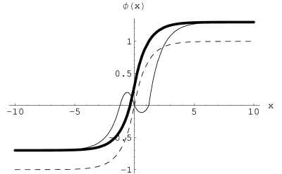
Figure 2: Kinklike solutions. The dashed line corresponds to the solution presented by Theodorakis for the case where $\epsilon=0$. The thick line is the profile of that configuration in the asymmetrical case, and the thin line is the new kink (Eq. (3)), both plotted using $\epsilon=0.3$.

The above kink-like configuration is represented in Fig. 2. Note however that, in order to be sure that the first derivative of the field configuration is continuous at the intermediate point, one must constrain the distance between those points when $0<\epsilon<1$ through the relation

$$\frac{1-\cosh(x_{2}-x_{1})}{\sinh(x_{2}-x_{1})}=\frac{\epsilon-1}{\epsilon+1}=\frac{1-\cosh(x_{3}-x_{2})}{\sinh(x_{3}-x_{2})},$$ (4)

which, after some algebraic manipulations, is equivalent to require that

$$x_{2}-x_{1}=x_{3}-x_{2}=ArcCoth\left(\frac{1+\epsilon^{2}}{1-\epsilon^{2}}\right).$$ (5)

Here, it is important to remark that the case where $\epsilon=0$ can not be recovered from the one with $0<\epsilon<1$. In this particular situation, one can see that the differences $x_{2}-x_{1}$ and $x_{3}-x_{2}$ become equal to zero and we reproduce the case considered in [31].

Now, performing the analysis of the linear stability of this new solution by using the usual procedure [17], one ends with the following transcendental equation

$$\frac{\alpha}{2}\left[1-\frac{1}{\omega(1-\epsilon)}\right]e^{2\omega x_{2}}-\frac{1}{\omega(1-\epsilon)}\left[1-\frac{\alpha}{2}\right]+$$

$$\left.-\left(\frac{2+\beta}{\beta}\right)\left\{\frac{\left(\alpha+2\right)}{2}\left[1-\frac{1}{\omega(1-\epsilon)}\right]+\frac{\alpha e^{-2\omega x_{3}}}{2\omega(1-\epsilon)}\right\}e^{\omega x_{3}}=0,\right.$$ (6)

with $\omega=\sqrt{1-E}$, $\alpha\equiv-2/(\omega\left|d\phi_{2}/dx\right|_{x=x_{2}})$ and $\beta\equiv-2/(\omega\left|d\phi_{3}/dx\right|_{x=x_{3}})$. For instance, by analyzing an example where $\epsilon=0.367$, one can verify that there are two solutions with negative energies $E=-10.7113$ and $E=-1.49798$. This implies that the solution is unstable.

Once again, it was possible to find a kink-like solution, but this time presenting an oscillating region which can become larger if one introduces more regions in the game, as we are going to see later.

Since the model presents these two vacua, one can ask for other analytical solutions connecting a given vacuum to itself. In fact, one can construct two of these solutions, one for the false vacuum and another for the true one.

Below, we will determine a solution which presents three regions, beginning and ending at the true vacuum. In certain sense this solution completes the simplest set of lumps or critical bubbles which were introduced by Theodorakis in [31] (starting and finishing at the false vacuum). In Fig. 3, it can be seen a plot of both ours and the Theodorakis solutions.

Now, the field $\phi$ in each one of the regions will behave respectively as $\phi_{I}>0$, $\phi_{II}<0$ e $\phi_{III}>0$. In this case, we can show that it is a stable solution, in contrast with the one analyzed by Theodorakis. In other words, the lump connecting the true vacuum to itself is stable and the one related to the false vacuum is not. Thus, by making an analysis similar to that one done by Theodorakis, we can interpret this result in the sense that there is a stable portion of false vacuum among two regions of true vacua.

Furthermore, we are interested in constructing more complex solutions, where the size of the region separating the true and the false vacua is larger. For this, we introduce an entire new class of solutions, where the field oscillates between the true and the false vacua regions. Let us present an example with five regions such that $\phi_{I}<0$, $\phi_{II}>0$, $\phi_{III}<0$, $\phi_{IV}>0$ and $\phi_{V}<0$. Again, the points $x_{1}$, $x_{2}$, $x_{3}$ and $x_{4}$ correspond to zeros of $\phi(x)$.

With this in mind, it is not difficult to conclude that  one should have the following solution

$$\phi_{I}(x) = (1-\epsilon)(e^{x-x_{1}}-1),$$

$$\phi_{II}(x) = (1+\epsilon)\left[1-\frac{\sinh(x-x_{1})}{\sinh(x_{2}-x_{1})}-\frac{\sinh(x_{2}-x)}{\sinh(x_{2}-x_{1})}\right],$$

$$\phi_{III}(x) = -(1-\epsilon)\left[1-\frac{\sinh(x-x_{2})}{\sinh(x_{3}-x_{2})}-\frac{\sinh(x_{3}-x)}{\sinh(x_{3}-x_{2})}\right],$$ (7)

$$\phi_{IV}(x) = (1+\epsilon)\left[1-\frac{\sinh(x-x_{3})}{\sinh(x_{4}-x_{3})}-\frac{\sinh(x_{4}-x)}{\sinh(x_{4}-x_{3})}\right]$$

$$\phi_{V}(x) = (\epsilon-1)(1-e^{x_{4}-x}).$$

This is the case in which we apply our idea to the case explored by Theodorakis, when he was considering the critical bubble in the false vacuum. The difference is that, now, the field configuration starting at the false vacuum, before going back to it, oscillates once between the positive and negative vacua regions.

Verifying the stability of this new solution, one can see that the potential $V_{st}=1-2~{}\delta[\phi(x)]$, where

$$\delta[\phi(x)]=\frac{\delta(x-x_{1})}{\left|\frac{d\phi}{dx}\right|_{x=x_{1}}}+\frac{\delta(x-x_{2})}{\left|\frac{d\phi}{dx}\right|_{x=x_{2}}}+\frac{\delta(x-x_{3})}{\left|\frac{d\phi}{dx}\right|_{x=x_{3}}}+\frac{\delta(x-x_{4})}{\left|\frac{d\phi}{dx}\right|_{x=x_{4}}}.$$ (8)

This time the equation used to find the energies of the bound states related to the perturbation is expressed as

$$\left\{\beta[1-(1+\gamma)]e^{2\omega x_{4}}-\gamma(1-\beta)\right\}\left\{\left(\frac{\alpha}{2}-1\right)\left[\frac{1}{\omega(\epsilon-1)}\right]\right.$$

$$\left.-\frac{\alpha}{2}\left[1+\frac{1}{\omega(\epsilon-1)}\right]e^{2\omega x_{2}}\right\}-\{(\beta+1)(\gamma+2)e^{2\gamma\omega x_{4}}-\beta\gamma e^{2\gamma\omega x_{3}}\}$$

$$\left.\times\left\{1-\left(\frac{\alpha}{2}-1\right)\left[\frac{1}{\omega(\epsilon-1)}\right]+\frac{\alpha}{2}\left[1+\frac{1}{\omega(\epsilon-1)}\right]e^{2\omega x_{2}}\right\}=0\right.$$ (9)

with

$$\alpha\equiv-\frac{2}{\omega\left|\frac{d\phi_{2}}{dx}\right|_{x=x_{2}}},~{}\beta\equiv-\frac{2}{\omega\left|\frac{d\phi_{3}}{dx}\right|_{x=x_{3}}}\text{ and }\gamma\equiv-\frac{2}{\omega\left|\frac{d\phi_{4}}{dx}\right|_{x=x_{4}}}.$$

From the equation (9) we get a negative value for the energy, signalizing that this configuration, as the one in [31], is unstable.

The corresponding configuration starting and finishing at the true vacuum is given by

$$\phi_{I}(x) =(1+\epsilon)(1-e^{x-x_{1}}),$$

$$\phi_{II}(x) =-(1-\epsilon)\left[1-\frac{\sinh(x-x_{1})}{\sinh(x_{2}-x_{1})}-\frac{\sinh(x_{2}-x)}{\sinh(x_{2}-x_{1})}\right],$$

$$\phi_{III}(x) =(1+\epsilon)\left[1-\frac{\sinh(x-x_{2})}{\sinh(x_{3}-x_{2})}-\frac{\sinh(x_{3}-x)}{\sinh(x_{3}-x_{2})}\right],$$ (10)

$$\phi_{IV}(x) =-(1-\epsilon)\left[1-\frac{\sinh(x-x_{3})}{\sinh(x_{4}-x_{3})}-\frac{\sinh(x_{4}-x)}{\sinh(x_{4}-x_{3})}\right]$$

$$\phi_{V}(x) =(1+\epsilon)(1-e^{x_{4}-x}).$$

These last two solutions are plotted in Fig. 4. Again, it is not difficult to verify that it is unstable.

3 Fluctuating solitons in two and three dimensions

In two spatial dimensions, the spherically symmetric static configurations of the ADQ model must obey the equation

$$\frac{\partial^{2}\phi}{\partial r^{2}}+\frac{1}{r}\frac{\partial\phi}{\partial r}=\phi-\frac{\phi}{\left|\phi\right|}-\epsilon,$$ (11)

where $r=\sqrt{x^{2}+y^{2}}$. Thus, when $r\longrightarrow\infty$ the field $\phi\longrightarrow\epsilon-1$.

Now, we construct a solution with four distinct solutions. These regions are, once again, characterized by $0\leq\phi_{1}\leq r_{1}$, $r_{1}\leq\phi_{2}\leq r_{2}$, $r_{2}\leq\phi_{3}\leq r_{3}$, $r_{3}\leq\phi_{4}$, with $\phi_{1}>0$, $\phi_{2}<0$, $\phi_{3}>0$ e $\phi_{4}<0$. After imposing the continuity of the field in each transition point, one gets

$$\phi_{1}(r) = (1+\epsilon)\left[1-\frac{I_{0}(r)}{I_{0}(r_{1})}\right],$$

$$\phi_{2}(r) = (1-\epsilon)\left\{\frac{[K_{0}(r_{1})-K_{0}(r_{2})]I_{0}(r)+[I_{0}(r_{2})-I_{0}(r_{1})]K_{0}(r)}{K_{0}(r_{1})I_{0}(r_{2})-K_{0}(r_{2})I_{0}(r_{1})}+\right.$$ (12)

$$\left.-1\right\},$$

$$\phi_{3}(r) = (1+\epsilon)\left\{\frac{[K_{0}(r_{2})-K_{0}(r_{3})]I_{0}(r)+[I_{0}(r_{3})-I_{0}(r_{2})]K_{0}(r)}{K_{0}(r_{3})I_{0}(r_{2})-K_{0}(r_{2})I_{0}(r_{3})}+\right.,$$

$$\left.+1\right\},$$

$$\phi_{4}(r) = (\epsilon-1)\left[1-\frac{K_{0}(r)}{K_{0}(r_{3})}\right].$$

The functions $K_{0}(r)$ and $I_{0}(r)$ are the modified Bessel functions. This oscillating kink solution is represented in Fig. 5

The stability equation in this dimension is given by

$$\left(-\frac{d^{2}}{dr^{2}}-\frac{1}{r}\frac{d}{dr}+V_{st.}\right)\Theta(r)=E~{}\Theta(r),$$ (13)

where we have $V_{st}=1-2~{}\delta[\phi(r)]$.

By solving Eq. (13), we find a positive value for the ground state, indicating that this configuration in two dimensions is stable, so that, for a small initial perturbation the solution is kept finite when the time goes by. In fact, the value of the ground state solution of (13) found for this configuration is $E_{0}=0.324$ ($\epsilon=0.3$). It is important to remark that, in this case, the Theodorakis solution is also stable, having $E=~{}0.592$.

Let us end this section by taking into account the three-dimensional case. In this dimension the spherically symmetric static field configurations must obey the equation

$$\frac{\partial^{2}\phi}{\partial r^{2}}+\frac{2}{r}\frac{\partial\phi}{\partial r}=\phi-\frac{\phi}{\left|\phi\right|}-\epsilon,$$ (14)

where $r=\sqrt{x^{2}+y^{2}+z^{2}}$. Below we construct a solution which presents the same features of the one discussed in the previous case. After applying the continuity conditions, one can conclude that

$$\phi_{1}(r) = (1+\epsilon)\left[1-\frac{r_{1}}{r}\frac{\sinh(r)}{\sinh(r_{1})}\right],$$

$$\phi_{2}(r) = (\epsilon-1)\left[\frac{(r_{1}e^{r_{1}}-r_{2}e^{r_{2}})}{(e^{2r_{2}}-e^{2r_{1}})}\frac{e^{r}}{r}+\frac{(r_{2}e^{r_{1}}-r_{1}e^{r_{2}})}{2re^{r}}{csch}(r_{2}-r_{1})+\right.$$ (15)

$$\left.+1\right],$$

$$\phi_{3}(r) = (\epsilon+1)\left[\frac{(r_{3}e^{r_{3}}-r_{2}e^{r_{2}})}{(e^{2r_{2}}-e^{2r_{3}})}\frac{e^{r}}{r}+\frac{(r_{3}e^{r_{2}}-r_{2}e^{r_{3}})}{2re^{r}}{csch}(r_{3}-r_{2})+\right.$$

$$\left.+1\right],$$

$$\phi_{4}(r) = (1-\epsilon)\left[\frac{r_{3}}{r}e^{r_{3}-r}-1\right].$$

In order to determine the stability of the configuration, the equation to be solved in three spatial dimensions is written as

$$\left(-\frac{d^{2}}{dr^{2}}-\frac{2}{r}\frac{d}{dr}+V_{st.}\right)\Theta(r)=E\Theta(r),$$ (16)

and, again, $V_{st}=1-2~{}\delta[\phi(r)]$. In this case, we begin by obtaining the solution at each side of the transition points of the following equation

$$\frac{d^{2}\Theta}{dr^{2}}+\frac{2}{r}\frac{d\Theta}{dr}+(E-1)\Theta=0$$ (17)

so obtaining

$$\Theta_{1}(r) = C_{1}~{}r^{-1}\sin(r\sqrt{1-E}),$$

$$\Theta_{2}(r) = C_{2}~{}r^{-1}\sin(r\sqrt{1-E})+D_{2}~{}r^{-1}\cos(r\sqrt{1-E}),$$

$$\Theta_{3}(r) = C_{3}~{}r^{-1}\sin(r\sqrt{1-E})+D_{3}~{}r^{-1}\cos(r\sqrt{1-E}),$$

$$\Theta_{5}(r) = C_{5}~{}r^{-1}\sin(r\sqrt{1-E}).$$

On the other hand, the discontinuity at the transition points due to the presence of the Dirac delta function leads us to impose that

$$\left.r\frac{d\Theta}{dr}\right|_{r=r_{1}+\xi}-\left.r\frac{d\Theta}{dr}\right|_{r=r_{1}-\xi} = \frac{2r_{1}\Theta_{1}(r_{1})}{\left|\frac{d\phi_{1}}{dr}\right|_{r=r_{1}}},$$

$$\left.r\frac{d\Theta}{dr}\right|_{r=r_{2}+\xi}-\left.r\frac{d\Theta}{dr}\right|_{r=r_{2}-\xi} = \frac{2r_{1}\Theta_{2}(r_{2})}{\left|\frac{d\phi_{2}}{dr}\right|_{r=r_{2}}},$$ (19)

$$\left.r\frac{d\Theta}{dr}\right|_{r=r_{3}+\xi}-\left.r\frac{d\Theta}{dr}\right|_{r=r_{3}-\xi} = \frac{2r_{1}\Theta_{3}(r_{3})}{\left|\frac{d\phi_{3}}{dr}\right|_{r=r_{3}}},$$

where we have taken $\xi\longrightarrow 0$.

Using the continuity at each one of the transition points for the functions (18) and also the above three conditions, we finish with a transcendental equation defining a negative energy solution, showing that this configuration is, once more, unstable.

4 Lorentz invariant solutions for the oscillating configurations

Since the Lagrangian density we are dealing with is a Lorentz invariant one, we can look for configurations for the field $\phi$ depending on an invariant quantity like $x_{\mu}x^{\mu}=t^{2}-r^{2}$, where $r^{2}=\sum\limits_{i=1}^{N}x_{i}^{2}$, and $N$ stands for the number of spatial dimensions.

Following the work by Theodorakis [31], we look for a solution which describes a transition from the false to the true vacuum. As observed in the Introduction section, it can be related to a number of interesting physical systems. In this situation, the scalar field evolves to the value $\epsilon+1$ when $x_{\mu}x^{\mu}~{}\rightarrow\infty$ because, when this happens, the field approaches its true vacuum. Besides, it will be equal to $\epsilon-1$ if $x_{\mu}x^{\mu}~{}\rightarrow-~{}\infty$. As we are interested in the construction of a new family of configurations, we propose a scalar field $\phi$ with four regions, where $\phi_{I}<0$, $\phi_{II}>0$, $\phi_{III}<0$ and $\phi_{IV}>0,$ similarly to the case in which we have introduced the oscillating kink-like configuration.

First of all, we define the variable $s=t^{2}-r^{2}\equiv x_{\mu}x^{\mu}$. Thus, we will have regions where $t^{2}-r^{2}>0$ and $t^{2}-r^{2}<0$. For the case where $t^{2}-r^{2}>0$, the field equation is written as

$$\frac{\partial^{2}\phi}{\partial\chi^{2}}+\frac{N}{\chi}\frac{\partial\phi}{\partial\chi}+\phi-\frac{\phi}{\left|\phi\right|}-\epsilon=0,$$ (20)

where $\chi=\sqrt{t^{2}-r^{2}}=\sqrt{s}$. Otherwise, if $t^{2}-r^{2}<0$ we get

$$\frac{\partial^{2}\phi}{\partial\rho^{2}}+\frac{N}{\rho}\frac{\partial\phi}{\partial\rho}-\phi+\frac{\phi}{\left|\phi\right|}+\epsilon=0,$$ (21)

with $\rho=\sqrt{r^{2}-t^{2}}=\sqrt{-s}$.

The equations (20) and (21) lead us to the solutions

$$\phi(\chi) = \chi^{-p}[a_{1}J_{p}(\chi)+a_{2}Y_{p}(\chi)]+1+\epsilon,\text{ if }\phi>0\text{, }s^{2}>0$$

$$\phi(\chi) = \chi^{-p}[b_{1}J_{p}(\chi)+b_{2}Y_{p}(\chi)]-1+\epsilon,\text{ if }\phi<0\text{, }s^{2}>0$$

$$\phi(\rho) = \rho^{-p}[c_{1}K_{p}(\rho)+c_{2}I_{p}(\rho)]+1+\epsilon,\text{ if }\phi>0\text{, }s^{2}<0$$

$$\phi(\rho) = \rho^{-p}[d_{1}K_{p}(\rho)+d_{2}I_{p}(\rho)]-1+\epsilon,\text{ if }\phi<0\text{, }s^{2}<0$$

where $p\equiv(N+1)/2$.

After the analysis of the impact of the asymptotic conditions $\phi\longrightarrow\epsilon\pm 1$ when $x_{\mu}x^{\mu}~{}\rightarrow\pm~{}\infty$, and also considering that $\phi$ must be finite throughout the range of the validity of the variable $s$, we conclude that the roots of $\phi$ shall assume negative values, and we finish with

$$\phi\left(\rho\right) = \epsilon-1+d_{1}\rho^{-p}~{}K_{p}(\rho),\text{ }t^{2}-r^{2}<s_{1}$$

$$\phi(\rho) = \rho^{-p}[c_{1}~{}K_{p}(\rho)+c_{2}~{}I_{p}(\rho)]+1+\epsilon,\text{ }s_{1}<\text{ }t^{2}-r^{2}<s_{2}$$

$$\phi(\rho) = \rho^{-p}[d_{3}~{}K_{p}(\rho)+d_{4}~{}I_{p}(\rho)]-1+\epsilon,\text{ }s_{2}<\text{ }t^{2}-r^{2}<s_{3}$$ (23)

$$\phi(\rho) = 1+\epsilon+c_{3}~{}\rho^{-p}I_{p}(\rho),\text{ }s_{3}<\text{ }t^{2}-r^{2}<0$$

$$\phi(\chi) = 1+\epsilon+a_{1}~{}\chi^{-p}J_{p}(\chi),\text{ }t^{2}-r^{2}>0.$$

Now, imposing that at each transition point $\phi$ has a root and at same time granting the continuity at $s=0$, one gets

$$\phi\left(\rho\right) = (\epsilon-1)\left[1-\rho^{-p}(\rho_{1})^{p}\frac{K_{p}(\rho)}{K_{p}(\rho_{1})}\right],\text{ }t^{2}-r^{2}<s_{1}$$

$$\phi(\rho) = (\epsilon+1)\left\{\rho^{-p}\left[-\left(\rho_{1}^{p}+I_{p}(\rho_{1})\frac{\rho_{1}^{p}K_{p}(\rho_{2})-\rho_{2}^{p}K_{p}(\rho_{1})}{I_{p}(\rho_{2})K_{p}(\rho_{1})-I_{p}(\rho_{1})K_{p}(\rho_{2})}\right)\frac{K_{p}(\rho)}{K_{p}(\rho_{1})}\right.\right.$$

$$\left.\left.\left.+\left(\frac{\rho_{1}^{p}K_{p}(\rho_{2})-\rho_{2}^{p}K_{p}(\rho_{1})}{I_{p}(\rho_{2})K_{p}(\rho_{1})-I_{p}(\rho_{1})K_{p}(\rho_{2})}\right)I_{p}(\rho)\right]+1\right\},s_{1}<\text{ }t^{2}-r^{2}<s_{2}\right.$$

$$\phi(\rho) = (\epsilon-1)\left\{\rho^{-p}\left[\left(\rho_{2}^{p}+I_{p}(\rho_{2})\frac{\rho_{3}^{p}K_{p}(\rho_{2})-\rho_{2}^{p}K_{p}(\rho_{3})}{I_{p}(\rho_{3})K_{p}(\rho_{2})-I_{p}(\rho_{2})K_{p}(\rho_{3})}\right)\frac{K_{p}(\rho)}{K_{p}(\rho_{2})}\right.\right.$$

$$\left.\left.\left.+\left(\frac{\rho_{3}^{p}K_{p}(\rho_{2})-\rho_{2}^{p}K_{p}(\rho_{3})}{I_{p}(\rho_{3})K_{p}(\rho_{2})-I_{p}(\rho_{2})K_{p}(\rho_{3})}\right)I_{p}(\rho)\right]-1\right\},s_{2}<\text{ }t^{2}-r^{2}<s_{3}\right.$$

$$\phi\left(\rho\right) = (\epsilon+1)\left\{1-\rho^{-p}(\rho_{3})^{p}\frac{I_{p}(\rho)}{I_{p}(\rho_{3})}\right\},\text{ }s_{3}<\text{ }t^{2}-r^{2}<0$$

$$\phi(\chi) = (\epsilon+1)\left\{1-\chi^{-p}(\rho_{3})^{p}\frac{J_{p}(\chi)}{I_{p}(\rho_{3})}\right\},\text{ }t^{2}-r^{2}>0,$$

with $\rho_{1}=\sqrt{-s_{1}}$, $\rho_{2}=\sqrt{-s_{2}}$ and $\rho_{3}=\sqrt{-s_{3}}$. The points $\rho_{1},\rho_{2}$ and $\rho_{3}$ were found under the condition that at each transition between the regions the scalar field and its first derivative must be continuous. In Fig. 7, we present a comparison between the solution appearing in [31] and the one introduced in this work.

5 Conclusions

In summary, in this work we were able to construct a large class of new static configurations and, particularly, these solutions are such that the size of the wall between two regions of a given vacuum depends on the number of oscillations of the field. Furthermore, we also studied the stability of each of the solutions, observing that almost all of them are unstable, except by the two-dimensional kinks (bubbles in the Theodorakis nomenclature), and the lump connecting the true vacuum to itself in one spatial dimension. This lead us to conclude that the size of the solution does not determines its stability as suggested in [31]. Furthermore, as it can be seen from Fig. 6, our oscillating solutions are such that the corresponding domain walls becomes larger when one considers an increasing number of oscillations between the regions of false and true vacua. Thus, if one is analyzing the Lorentz invariant solutions, which evolve from the false to the true vacuum, it can be concluded that the time necessary for this transition is bigger for the higher oscillating configurations. It would be very interesting to see if such kind of richer structure is still present in the case of brane world dominated scenarios [23], similarly to what happens with the cosmological instantons [27].

Before ending the work, we note that one can obtain a generalized one-dimensional configuration having an arbitrary number of oscillating regions, which can be written as

$$\phi(x)=S(-x+x_{1})(\epsilon-1)(1-e^{x-x_{1}})+S(x-x_{n-1})(\epsilon+1)(1-e^{x_{n-1}-x})$$

$$+\sum_{m=2}^{n-1}\left\{S(x-x_{m-1})S(-x+x_{m})[\epsilon+(-1)^{m}]\right.$$ (25)

$$\left.\times[1-\frac{\sinh(x-x_{m-1})+\sinh(x_{m}-x)}{\sinh(x_{m-}x_{m-1})}\right\},~{}n\geqslant 3.$$

In the above generalization of the kink-like solution, $S(x)$ is the Heaviside function and $n$ stands for the number of regions. Now, for the case of the lump (bubble) starting and finishing at the false vacuum, our general solution is represented by

$$\phi(x) =S(-x+x_{1})(\epsilon-1)(1-e^{x-x_{1}})+S(x-x_{n-1})(\epsilon-1)(1-e^{x_{n-1}-x})$$

$$+\sum_{m=2}^{n-1}\left\{S(x-x_{m-1})S(-x+x_{m})[\epsilon+(-1)^{m}]\right.$$ (26)

$$\left.\times[1-\frac{\sinh(x-x_{m-1})+\sinh(x_{m}-x)}{\sinh(x_{m-}x_{m-1})}\right\},~{}n\geqslant 3.$$

Finally, the corresponding generalization for the configuration starting and finishing at the true vacuum is given by

$$\phi(x)=S(-x+x_{1})(\epsilon-1)(1-e^{x-x_{1}})+S(x-x_{n-1})(\epsilon+1)(1-e^{x_{n-1}-x})$$

$$+\sum_{m=2}^{n-1}\left\{S(x-x_{m-1})S(-x+x_{m})[\epsilon+(-1)^{m}]\right.$$

$$\left.\times[1-\frac{\sinh(x-x_{m-1})+\sinh(x_{m}-x)}{\sinh(x_{m-}x_{m-1})}\right\},~{}n\geqslant 3.$$ (27)

The solutions (26) and (27) are represented in Fig. 6.

The two-dimensional case is written  as

$$\phi(r) =S(r)S(-r+r_{1})(\epsilon+1)\left[1-\frac{I_{0}(r)}{I_{0}(r_{1})}\right]$$

$$+S(r-r_{n-1})(\epsilon-1)\left[1-\frac{K_{0}(r)}{K_{0}(r_{n-1})}\right]$$

$$+\sum_{m=2}^{n-1}S(r-r_{m-1})S(-r+r_{m})[\epsilon+(-1)^{m-1}]\left\{(-1)^{m-1}\right.$$

$$\left.+\frac{[K_{0}(r_{m-1})-K_{0}(r_{m})]I_{0}(r)+[I_{0}(r_{m})-I_{0}(r_{m-1})]K_{0}(r)}{K_{0}(r_{m})I_{0}(r_{m-1})-K_{0}(r_{m-1})I_{0}(r_{m})}\right\},~{}n\geqslant 3.$$ (28)

Finally, the case of three dimensions is such that

$$\phi(r) =S(r)S(-r+r_{1})(\epsilon+1)\left[1-\frac{r_{n}}{r}\frac{\sinh(r)}{\sinh(r_{1})}\right]$$

$$+S(r-r_{n-1})(1-\epsilon)\left(\frac{r_{n-1}e^{r_{n-1}-r}}{r}-1\right)$$

$$+\sum_{m=2}^{n-1}\left\{S(r-r_{m-1})S(-r+r_{m})[\epsilon+(-1)^{m-1}]\left[-\frac{(r_{m}e^{r_{m}}-r_{m-1}e^{r_{m-1}})}{(e^{2r_{m}}-e^{2r_{m-1}})}\frac{e^{r}}{r}\right.\right.$$

$$\left.\left.+\frac{(r_{m}e^{r_{m-1}}-r_{m-1}e^{r_{m}})}{2re^{r}}\right]\cosh(r_{m-r_{m-1}})+1\right\},~{}n\geqslant 3.$$ (29)

Acknowledgements: The authors thanks to CNPq and FAPESP for partial financial support. ASD also give thanks to Professor D. Bazeia for introducing him to the matter of solitons and BPS solutions. This work was partially done during a visit (ASD) within the Associate Scheme of the Abdus Salam ICTP.

Figure 1: Potential of the asymmetrical doubly-quadratic (ADQ) model for $\epsilon=0.3$.

Figure 3: Lumplike solutions (bubble) in one dimension for $\epsilon=0.3$. The dashed line is the solution presented by Theodorakis for a configuration starting and finishing at the false vacuum and the solid line is our solution connecting the true vacuum to itself.

Figure 4: Lumplike solutions (bubble) with two oscillations for $\epsilon=0.3$.

Figure 5: Oscillating configuration in two dimensions for $\epsilon=0.3$. The dashed line corresponds to the case studied in [31].

Figure 6: Generalization of the kinklike (dashed line) and lumplike (solid line) solutions with $\epsilon=0.3.$

Figure 7: Lorentz invariant solution for $\epsilon=0.2828225347021907$. The dashed line is the solution presented by Theodorakis and the solid line is the one introduced here.