Rotating inclined cylinder and the effect of the tilt angle on vortices

Abstract

We study numerically some possible vortex configurations in a rotating cylinder that is tilted with respect to the rotation axis and where different numbers of vortices can be present at given rotation velocity. In a long cylinder at small tilt angles the vortices tend to align along the cylinder axis and not along the rotation axis. We also show that the axial flow along the cylinder axis, caused by the tilt, will result in the Ostermeier-Glaberson instability above some critical tilt angle. When the vortices become unstable the final state often appears to be a dynamical steady state, which may contain turbulent regions where new vortices are constantly created. These new vortices push other vortices in regions with laminar flow towards the top and bottom ends of the cylinder where they finally annihilate. Experimentally the inclined cylinder could be a convenient environment to create long lasting turbulence with a polarization which can be adjusted with the tilt angle.

I Introduction

Under uniform rotation the equilibrium state of a superfluid consists of a regular array of rectilinear quantized vortices along the rotation axis. This is strictly true only when the top and bottom plates of the rotating container are perpendicular to the rotation axis and its cross section has fixed translationally invariant form along the rotation axis. Near the walls that are parallel to the rotation axis the vortex array is surrounded by a small vortex free layer of thickness that is of the order of the vortex spacingfetterSurf ; donnellySurf .

The usual setup to study vortices in rotation is to use a cylindrical container and to assume that the cylinder axis is aligned exactly parallel to the rotation axis. Nevertheless, experimentally the rotation axis is always tilted by some small unknown angle owing to uncontrolled mechanical misalignment. Even if the misalignment is small, one is tempted to ask the question: What is the effect of the tilt and how does it affect the steady state vortex configuration? Fortunately, it turns out that cylindrical symmetry is not immediately broken at any arbitrarily small tilt angle. A sensitive test of the tilt angle is the measurement of the number and configuration of vortices in the equilibrium state of rotationRuutu1998 , particularly the relative number of the centrally located rectilinear vortices and the curved peripheral vortices which have one or both ends on the cylindrical side wall. During changes of the rotation velocity $\Omega$ the curved peripheral vortices behave very differently from the central rectilinear vortices: They have no annihilation energy barrierRuutu1998 during a deceleration of $\Omega$, while during acceleration they may become unstable with respect to loop formation and reconnection at the cylindrical side wall which leads to the generation of new independently evolving vortices in the increased rotational flowprecursorPRL .

For simple flow geometries at low velocities vortex filament calculations are today a reasonably efficient and reliable way to find the resulting vortex configurations, in many cases with less effort than by direct measurement. The rotating inclined cylinder is a good example since an extensive series of measurements would be needed to scan the behavior as a function of tilt angle, rotation velocity, and mutual friction. Here we are not attempting to provide the entire quantitative picture of the possible flow states, but look for the main qualitative changes from the ideal case.

Already in the 1980’s Mathieu et al.mathieu considered a cavity that was tilted with respect to the rotation axis. They used the free-energy principle combined with the HBVK continuum approximation. They also implicitly assumed that far from the boundaries the vortices are aligned along the rotation axis, and considered a rectangular cavity which is infinite in one direction (that is perpendicular to the rotation axis). In the rectangular geometry considered by Mathieu et al.mathieu the superfluid velocity without vortices is always along the direction which is considered to to be infinitely long. This forces the vortices to lie in the plane perpendicular to this direction. In reality the cavities are not infinitely long and often the longest dimension is oriented along the rotation axis. Therefore the flow of the superfluid component without vortices takes a more complicated form. Unless the container has rotational symmetry and its symmetry axis is aligned perfectly along the rotation axis, the superfluid is not at rest any more but moves due to the container boundaries. This results in that the superfluid velocity is not simply caused by vortices but contains a potential part that must be taken into account.

In the following we consider a circular cylinder and find its vortex configuration in rotation using the vortex filament model. The stable vortex configuration is obtained by following the evolution in the vortex dynamics long enough in order to obtain the steady state response. The most striking result, which differs from the general view and from the results assumed in Ref. mathieu , is that far from boundaries the vortices may tend to align not along the rotation axis but along the symmetry axis of the rotating cylinder. This is especially true for a single vortex under high rotation and for an array with a large number of vortices. These configurations would result if the cylinder with a given number of straight vortices is tilted by an angle which is less than a critical value. With large enough tilt angles the vortices may become unstable and tend to orient more along the rotation axis. Above the critical angle there exist turbulent regions in the tilted cylinder which act as a source for new vortices. Therefore the tilt of the cylinder has a similar effect as rotation around more than one axisKobayashi .

The article is organized as follows. First in Sec. II we solve the velocity profile for the superfluid component inside the cylinder when no vortices are present. In the following section we describe briefly the vortex filament model and the numerical procedure that is used to determine the vortex motions and the steady state inside the cylinder. Section IV is devoted to the results.

II Motion of the ideal fluid inside tilted rotating cylinder

Figure 1: Cylinder tilted by an angle $\eta$ with respect to the rotation axis $\bm{\Omega}=\Omega\hat{\bf Z}$.

The helium superfluids, ⁴He and ³He, can be described using a two-fluid model where the superfluid part behaves like an ideal Eulerian fluid with negligible viscosity and the normal component behaves like a classical fluid with finite viscosity. We are mostly interested in superfluid ³He-B, where the normal component is very viscous and can always be considered to be in solid body rotation in the rotating cavity. If there are no vortices, the superfluid part is in potential flow, which must be taken into account before one can consider the motion of the vortices. In case of an ideal circular cylinder, with radius $R$ and length $L$, aligned perfectly along the rotation axis, the superfluid remains stationary in the laboratory frame. When the cylinder axis is not parallel to the rotation axis the superfluid is no more at rest but is put into motion due to the boundaries. The same occurs also in all other cases without cylindrical symmetry, such as the rotating boxMT or a cylinder with ellipsoidal cross sectionLL . Consider a situation (at some particular time) illustrated in Fig. 1 where $\bm{\Omega}=\Omega\hat{\bf Z}$ and the cylinder axis is along $\cos\eta\hat{\bf Z}+\sin\eta\hat{\bf X}$. At that particular time the fixed Cartesian coordinates $(X,Y,Z)$, denoted by uppercase letters, and the Cartesian coordinates $(x,y,z)$, fixed to the rotating cylinder and denoted by lowercase letters, can be related by a rotation by an angle $\eta$ around the $Y$-axis. The cylindrical coordinates $(\rho,\phi,z)$ that are also fixed to the rotating cylinder, such that $\rho=\sqrt{x^{2}+y^{2}}$ and $\phi=\arctan(y/x)$, can then be related to the fixed laboratory coordinates via

$$X = \rho\cos\phi\cos\eta+z\sin\eta$$

$$Y = \rho\sin\phi$$ (1)

$$Z = -\rho\cos\phi\sin\eta+z\cos\eta.$$

The boundaries of the cylinder are given by the surfaces $\rho=R$ and $z=\pm{L}/2$. In cylindrical coordinates $\bm{\Omega}$ and ${\bf r}$ are given by

$$\bm{\Omega} = \Omega\left[-\sin\eta\cos\phi\hat{\bm{\rho}}+\sin\eta\sin\phi\hat{\bm{\phi}}+\cos\eta\hat{\bf{z}}\right]$$ (2)

$${\bf r} = \rho\hat{\bm{\rho}}+z\hat{\bf{z}}.$$ (3)

Without vortices the superfluid velocity follows that in potential flow, ${\bf v}=\nabla\Phi$, where the potential $\Phi$ satisfies the Laplace equation. The boundary condition is that at the surfaces (with normal $\hat{\bf n}$) the velocity component normal to the boundary satisfies $\frac{\partial\Phi}{\partial{n}}=\hat{\bf n}\cdot(\bm{\Omega}\times{\bf r})$ which implies that one must solve the following system of equations:

$$\frac{1}{\rho}\frac{\partial}{\partial{\rho}}\left(\rho\frac{\partial\Phi}{\partial{\rho}}\right)+\frac{1}{\rho^{2}}\frac{\partial^{2}\Phi}{\partial\phi^{2}}+\frac{\partial^{2}\Phi}{\partial{z}^{2}} = 0$$ (4)

$$\frac{\partial\Phi}{\partial{\rho}}_{|_{\rho=R}}=\Omega{z}\sin\eta\sin\phi,\hskip 11.38109pt\frac{\partial\Phi}{\partial{z}}_{|_{z=\pm\frac{L}{2}}} = -\Omega\rho\sin\eta\sin\phi.$$

The above equations give the solution in the laboratory frame. Conversion to the rotating frame is obtained by removing the effect of rotation, so that the velocity is given by

$${\bf v}=\nabla\Phi-\bm{\Omega}\times{\bf r}.$$ (5)

Equation (4) can be further simplified with the use of a trial function $\Phi(\rho,\phi,z)$ $=$ $\Omega(\rho z+g(\rho,z))\sin\phi\sin\eta$, which results in that $g(\rho,z)$ has to satisfy the following Helmholtz equation:

$$\frac{1}{\rho}\frac{\partial}{\partial{\rho}}\left(\rho\frac{\partial{g}}{\partial{\rho}}\right)+\frac{\partial^{2}{g}}{\partial{z}^{2}}-\frac{1}{\rho^{2}}g = 0$$

$$\frac{\partial{g}}{\partial{\rho}}_{|_{\rho=R}}=0,\hskip 14.22636pt\frac{\partial{g}}{\partial{z}}_{|_{z=\pm\frac{L}{2}}} = -2\rho.$$

Note that the potential $g(\rho,z)$ does not depend on tilt angle $\eta$. The velocity components in the rotating frame, obtained from Eq. (5), are then given by

$$v_{\rho} = \Omega\sin\phi\sin\eta\frac{\partial g}{\partial\rho}$$

$$v_{\phi} = \Omega\cos\phi\sin\eta\frac{g}{\rho}-\Omega\rho\cos\eta$$ (6)

$$v_{z} = \Omega\sin\phi\sin\eta(2\rho+\frac{\partial g}{\partial{z}}).$$

One notices that the tilt of the cylinder implies a flow parallel to the cylinder axis and also reduces the azimuthal counterflow. The axial velocity is largest at the cylinder wall ($\rho=R,z=0$) and varies as $\sin\phi$ as one goes around the cylinder axis. The solution to the above equations is found numerically, except in case of an infinitely long cylinder, when $g=0$. As an example, the solution for the vortex-free flow state is plotted in Fig. 2 for the potential $g(\rho,z)$ and in Fig. 3 for the velocity $v(x,y,z)$, when $L/R=4$ and $\eta=30^{\circ}$.

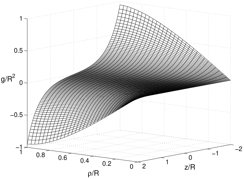
Figure 2: Solution for velocity potential $g(\rho,z)$ when $L=4R$.

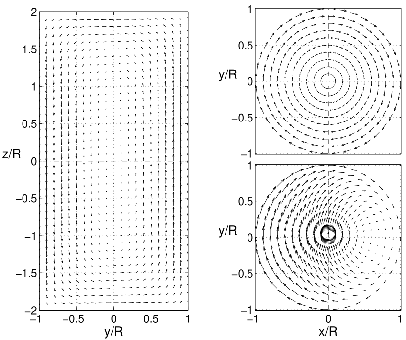
Figure 3: Velocity in the rotating cylinder when $L=4R$ and when the angle between the rotation axis and cylinder axis, $\eta=30^{\circ}$. Left: Velocity in the $x=0$ plane, the plane that is perpendicular to the plane defined by the cylinder and the rotation axes. Right top: Velocity in the $z=0$ plane. Right bottom: Velocity in the bottom of the cylinder, $z=-L/2$. The coordinates $(x,y,z)$ are fixed to the rotating cylinder.

III Vortex filament model

Superfluid vortices are modeled as line defects. This model is suitable especially for superfluid ⁴He where the core diameter is of the order of atomic size. Our calculations are attempting to model primarily superfluid ³He-B where two simplifications can be assumed: 1) The normal fraction is always in solid-body rotation with the container, as noted in Sec. II. 2) In addition the core diameter $a_{0}\approx 10^{-5}$ mm. This is still a small value compared to the experimental dimensions of a few millimeters and the use of the vortex filament model is appropriate. The larger coresize, however, makes it more justifiable to assume smooth walls for the cylinder, since so far there has been no clear experimental indication that vortices become pinned if the walls of the container are well polishedPLTP16 . Also down to intermediate temperatures of $T\gtrsim 0.4T_{c}$ mutual friction damping is sufficiently high so that vortices are rapidly annihilated at zero flow conditions. In such conditions vortex remanence is not a major problem and relatively large vortex-free normal fluid-superfluid counterflow can be achieved. In practice this means that the rotating container can generally be filled with any number of vortices up to the number which corresponds to the equilibrium state with solid-body rotation of the superfluid componentRuutu1997 .

The vortex filament model is well described by Schwarz in Refs.schwarz85 ; schwarz88 . Our numerical scheme is similar. Line vortices are described by a sequence of points $\{{\bf s}_{i}\}_{i=0}^{M}$. The required tangent, curvature radius etc. at some particular point ${\bf s}({\bf r})$ along the line vortex are calculated by fitting a circle through three points (the point under consideration and the nearest neighbours). The main difference, compared to calculations of Schwarz, is that we use a 4th order Runge-Kutta method to determine the vortex motion that is described by the following equation:

$${\bf v}_{\rm L}={\bf v}_{\rm s}+\alpha\hat{\bf s}^{\prime}\times({\bf v}_{\rm n}-{\bf v}_{\rm s})-\alpha^{\prime}\hat{\bf s}^{\prime}\times[\hat{\bf s}^{\prime}\times({\bf v}_{\rm n}-{\bf v}_{\rm s})]\,.$$ (7)

Here ${\bf v}_{\rm L}=d{\bf s}/dt$ is the velocity of the vortex point at ${\bf s}$ with unit tangent $\hat{\bm{s}}^{\prime}$. The above equation includes the mutual friction between vortex lines and the normal fluid with coefficients $\alpha$ and $\alpha^{\prime}$ that are taken as a function of temperature from the measurements of Bevan et al.Bevan ; BevanPRL This equation is typically used in the laboratory frame where ${\bf v}_{\rm n}=\bm{\Omega}\times{\bf r}$, but is also valid in the rotating frame where ${\bf v}_{\rm n}=0$.sonin Now in the rotating frame the superfluid velocity ${\bf v}_{\rm s}={\bf v}+{\bf v}_{\omega}+{\bf v}_{\rm b}$ consists of the velocity due to rotation, ${\bf v}$, calculated above in Sec. II and given by Eq. (II), the superfluid velocity due to vortices, ${\bf v}_{\omega}$, and the boundary induced velocity, ${\bf v}_{\rm b}$, that is needed to cancel the velocity through the boundaries due to vortices.

As one may notice the above method for doing the calculation in the rotating frame differs from previous simulations in Refs.nature ; TsubotaPRB2004 ; TsubotaPRL2003 , which contain a complicated term, $\dot{\bf s}_{\rm rot}$, that was used to take into account the rotation. This earlier approach cannot be completely correct. A simple way to check this is to consider the zero temperature limit in an infinite system with no other external velocities (except the rotation of the normal component, which at $T=0$ cannot couple to the vortex motion, simply because it is absent). In this case our ${\bf v}$ reduces to ${\bf v}=-\bm{\Omega}\times{\bf r}$ and that takes care of the rotating frame. This term does not change the vortex configuration, but just rotates the coordinates, like expected. However, the term $\dot{\bf s}_{\rm rot}$ may have a more dramatic change on the vortex configuration since the term depends on the vortex configuration itself. Therefore, owing to its complex form, this term has different and configuration-dependent consequences.

The superfluid velocity due to vortices is obtained using the Biot-Savart formulation:

$${\bf v}_{\omega}({\bf r},t)=\frac{\kappa}{4\pi}\int\frac{({\bf s}_{1}-{\bf r})\times d{\bf s}_{1}}{|{\bf s}_{1}-{\bf r}|^{3}}.$$ (8)

Here the integration is a line integral along the vortices and $\kappa$ is the quantum of circulation. When ${\bf r}={\bf s}$ is one of the vortex points, the above equation becomes singular as ${\bf s}_{1}\rightarrow{\bf s}$. This singularity can be avoided, for example, by considering a moving vortex ring schwarz85 . If one denotes with $l_{-}$ and $l_{+}$ as being the lengths of two adjacent line elements connected to the point ${\bf s}$, then the velocity of this point is given by

$${\bf v}_{\omega}({\bf s},t) = \frac{\kappa}{4\pi}\hat{\bf s}^{\prime}\times{\bf s}^{\prime\prime}\ln\left(\frac{2\sqrt{l_{+}l_{-}}}{e^{1/4}a_{0}}\right)$$ (9)

$$+ \frac{\kappa}{4\pi}\int^{{}^{\prime}}\frac{({\bf s}_{1}-{\bf s})\times d{\bf s}_{1}}{|{\bf s}_{1}-{\bf s}|^{3}}.$$

The integral (the term that is typically denoted as the non-local term) is now taken over the rest of the vortex filament, not connected to the point ${\bf s}$. Vectors $\hat{\bf s}^{\prime}$ and ${\bf s}^{\prime\prime}$ in the local term are the tangent and principal normal at ${\bf s}$ and the derivation is with respect to the arc length, $\xi$, along the vortex.

As already described by Schwarz, the boundary velocity, ${\bf v}_{\rm b}=\nabla\Phi_{\rm b}$, in general, must be obtained by solving the Laplace equation $\nabla^{2}\Phi_{\rm b}=0$ with the boundary condition that $\hat{\bf n}\cdot({\bf v}_{\omega}+{\bf v}_{\rm b})=0$ on the boundary, with normal $\hat{\bf n}$. This method has been used in several previous calculations, for example in Ref. twistPRL , by using finite differences to discretize the Laplace equation and solving the resulting sparse matrix equation. The resulting matrix is typically very large and limits the grid size that can be used to evaluate the boundary velocity. In these calculations here we used an approximate method, namely image vortices to evaluate the boundary velocity. Above and below the cylinder we used simple image vortices to cancel the velocity through the bottom and top plates of the cylinder. The velocity through the cylindrical wall at $\rho=R$ is canceled using an inverse image curve where the distance of the image vortex from the cylinder axis is given by $\rho_{\rm im}=R^{2}/\rho$. Here $\rho$ is the distance of the vortex from the axis. The $z$ and $\phi$ coordinates of the image vortex are the same as those for the real vortex (additionally one needs to reverse the direction of the image vortex). A similar method was used by Zieve and DonevZieve . This image vortex method is accurate in case of straight vortices parallel to the cylinder axis. When comparing the simulations with the full solution of the Laplace equation, the agreement is quite good since only a minor part of the velocity comes from the image field.

The vortex filament model cannot describe vortex reconnection processes and tell when a reconnection occurs. We use commonly accepted criteria for making a reconnection: A reconnection in simulations is done when two vortices approach each other closer than some small distance. This distance, denoted by $h_{\rm rec}$, is typically taken to be about one half of the smallest space resolution used to describe the vortices, $h_{\rm min}$. Additionally, we require that in every reconnection the vortex length must decrease, which approximately indicates that the total energy decreases. This additional requirement will prevent, for example, two parallel straight vortices from reconnecting. The distance between vortices is calculated, not simply by determining the distance between the points, but by calculating the smallest distance between different vortex segments. These vortex segments (extending from ${\bf s}_{i}$ to ${\bf s}_{i+1}$ are assumed to be straight. Reconnection with a cylinder wall is assumed to occur when a vortex is closer than $h_{\rm rec}/2$ from the wall. For plane boundaries this means that the distance to the image vortex is smaller than $h_{\rm rec}$ used for bulk reconnections. When a reconnection is done, the point closest to the wall is split into two and both these points (one being the first point on a vortex and the other one being the last point) are moved to the surface. The point separation along the vortex is kept between some reasonable limits, such that $h_{\rm min}<|{\bf s}_{i+1}-{\bf s}_{i}|<h_{\rm max}$ and more points are used in regions where the vortex is strongly curved. At the boundaries the vortex tangent is fixed to be along the surface normal. This requirement ensures that there is no flow through the surface. Small vortex loops are removed when it becomes impossible to follow their dynamics. In our numerical scheme this is implemented by removing any closed loop or vortex terminating on the wall which is shorter than $4h_{\rm min}$.

IV Results

IV.1 Configuration of a single vortex

Before analysing how a vortex array behaves in the tilted cylinder it is informative to consider a single vortex. The stability of the vortex with respect to creation of new vorticesprecursorPRL depends on mutual friction $\alpha(T)$ but also on the initial configuration (which in many experiments is unknown). The lower the temperature, the more easily a vortex becomes unstable, leading to the creation of a new vortex after reconnection at the boundary. All this is consistent with experimentsprecursorPRL ; nature . However, with zero tilt angle $\eta$ only very few configurations lead to multiplication of vortices, see for example Refs. simu ; precursorPRL . Therefore, to investigate the propagating vortex frontfrontPRL and the twisted vortex statetwistPRL behind it, the simulations had to be started with a large number of vortices. At low temperatures with small mutual friction our simulations show that the probability for a vortex to become unstable increases as the tilt angle increases from zero. In order to observe easy vortex multiplication (for various initial configurations) the tilt angle should be much larger than the experimental one, which is only of order one degree.

                    

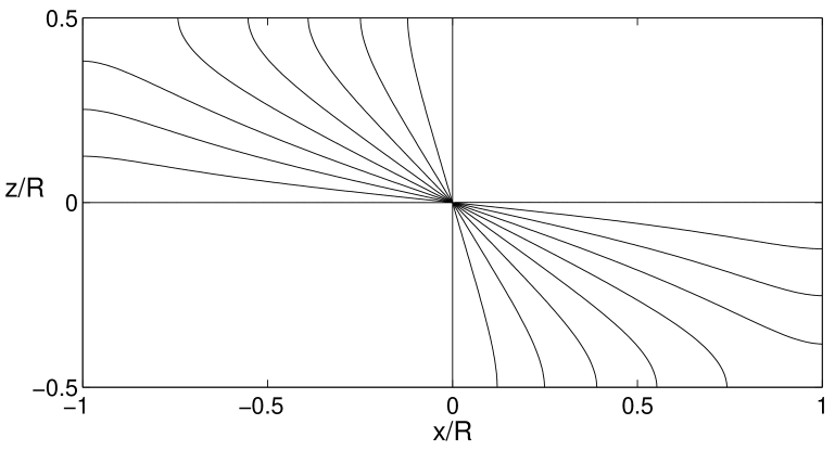
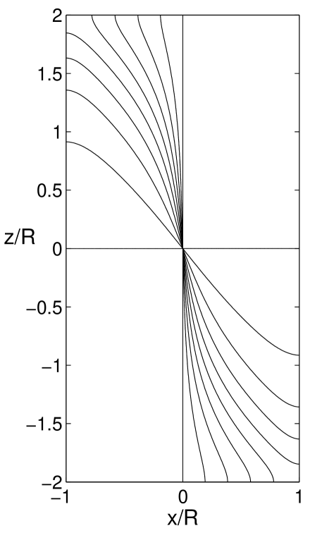
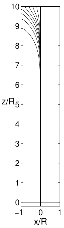
Figure 4: Configuration of a single vortex in the tilted rotating cylinder at a high rotation velocity of $\Omega=500$ mrad/s and radius $R$ = 3 mm. Tilt angles are $\eta=0,10,20,\ldots,$ and $90$ degrees. The vortex is practically in the $xz$-plane that is defined by the rotation and cylinder axes. Top: $L=R$. Bottom left: $L=4R$. Bottom right: $L=20R$, only the upper half of the vortex configuration is plotted.

In this article we are not focusing on the criteria for the vortex stability with respect to reconnection on the wall and the formation of independently moving new loops. These criteria seem to depend on many different features and parameters (at least on tilt angle, temperature, rotation velocity and initial vortex configuration). We are interested in the (possibly metastable) steady states in the cylinder, with different number of vortices in the cylinder.

The easiest way to find the steady state configurations of a single vortex is to start with the vortex along the cylinder axis with zero tilt. Then by increasing the tilt angle (which was done in Fig. 4 in steps of 10 degrees) one may follow the vortex dynamics by iterating Eq. (7) until the vortex finds its equilibrium position. To speed up the process and to avoid vortex multiplication these simulations were done at high enough temperatures, with the ³He-B parameter values at $T=0.8T_{c}$. The numerical resolution for these single vortex calculations was such that $h_{\rm min}$ = 0.04 mm and $h_{\rm max}$ = 0.10 mm. The cylinder radius was fixed to R = 3 mm.

For large rotation velocities there was no indication of hysteresis, i.e. the obtained configuration was the same even if one started the iteration from a straight vortex perpendicular the cylinder axis. The steady state configurations for high rotation velocity are illustrated in Fig. 4. One may notice that for a single vortex the steady state depends strongly on the aspect ratio $L/R$ of the cylinder. For short cylinders $L\sim R$ the vortex is approximately along the rotation axis, except near boundaries, where the vortex must be along the surface normal. For long cylinders, $L\gg R$, the vortex lies mainly along the cylinder axis and only deviates from this near the bottom and top plates. When $\eta\rightarrow 90^{\circ}$ the vortex finally turns and aligns itself along the rotation axis. For long cylinders the vortex is along the cylinder axis because then the azimuthal counterflow is reduced in a longer region, even if the reduction at every point is not an optimal one. For the short cylinder it is more important how well the counterflow is reduced locally and therefore a better result is obtained by orienting the vortex along the rotation axis. One should note that, with respect to the number of vortices, these single vortex states at high rotation velocities are metastable and far from equilibrium. However, they are experimentally accessible states in superfluid ³He-B, where at high temperatures one may easily create either a vortex free state or a state with an arbitrary number of vorticesRuutu1997 .

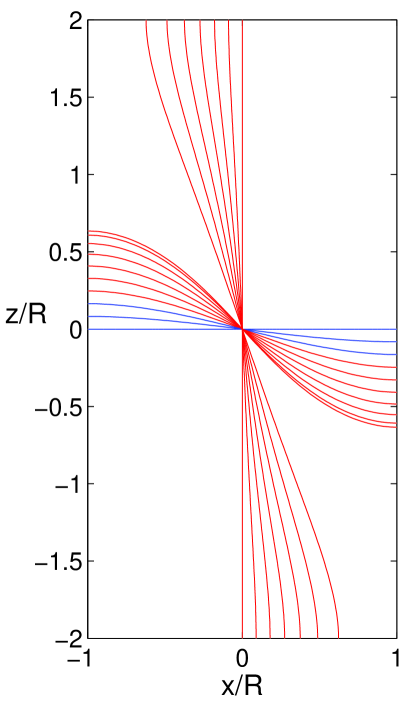
Figure 5: (Color online) Steady state vortex configurations for a single vortex in a tilted cylinder with $R$ = 3 mm and $L$ = 12 mm. The vortex is in the plane defined by the rotation and cylinder axes ($xz$-plane). Left: Low rotation velocity of 10 mrad/s. The tilt angles for vortices terminating to the top and bottom ends of the cylinder are: 0, 10, 20, 30, 40, 50, and 60 degrees and were obtained by increasing the tilt angle. The vortices terminating to the outer cell wall ($\rho=R$) correspond to tilt angles of 0, 10, $\ldots$, 90 and were obtained by decreasing the tilt from 90 degrees. The configurations for the highest tilt angles (from 70 to 90) can also be obtained by increasing the tilt. Right: Rotation velocity of 25 mrad/s. For vortices attached to the top and bottom plates of the cylinder the tilt angles are 0, 10, 20, $\ldots$, 60 degrees. For vortices terminating to the outer cell wall $\eta$ = 30, 40, $\ldots$, 90 degrees. Hysteresis in increasing/decreasing inclination is observed for angles 30, 40, 50, and 60 degrees.

At small rotation velocities one may observe hysteresis between different metastable configurations. This is quite natural since the boundary condition that a vortex must terminate perpendicular to the solid wall will result in a self-induced velocity due to its curvature that is of order $v_{\rm curv}=\kappa\ln(8R/a_{0})/4\pi{R}$, where $R$ is the radius of the cylinder. This translates to a characteristic rotation velocity of order 10 mrad/s at which hysteresis becomes important. This is illustrated in Fig. 5 where we have followed the vortex configuration by increasing the tilt angle first from zero to 90 degrees and then decreased it back to zero (also in steps of 10 degrees). Hysteresis also results from the cell geometry and the boundary requirement at the solid wall. Therefore a vortex may get trapped either on the top/bottom plate or on the cylindrical side wall, $\rho=R$, in a similar fashion as a vortex is trapped on a spherical pinning site on the plane boundaryschwarz85 .

IV.2 Vortex array in an infinitely long cylinder

When the rotation and cylinder axes are perfectly aligned, the vortices form a lattice of rectilinear lines which are parallel to the common axis. Closer to the cylindrical outer wall the vortex array deforms to concentric rings. These are separated from the cylinder wall by a vortex-free annulus which has a thickness of order of the intervortex distancefetterSurf ; donnellySurf ; Ruutu1998 . If one considers an infinitely long cylinder, which naturally is impossible to organize experimentally, but which gives a good hint of what might occur in a long cylinder far from the ends, some analytical results are possible. In this case the potential velocity profile due to the tilt is obtained by putting $g=0$ in Eq. (II). One may easily note that an array of rectilinear vortices along the cylinder axis can still be a stable solution. However, now the areal vortex density $n_{v}=2\Omega\cos\eta/\kappa$ is reduced by the factor $\cos\eta$ due to the reduced azimuthal counterflow in Eq. (II). The axial velocity $v_{z}$ in Eq. (II) does not affect the vortex configuration as long as it is below the critical value of the Ostermeier-Glaberson instabilityGJO ; Donnelly . Considering the stability of a single vortex and taking into account the maximum axial velocity $v_{\rm z,max}=2R\Omega\sin\eta$ and the reduced counterflow, one obtains that the vortices suffer the instability when $v_{\rm z,max}>2\sqrt{\nu\Omega\cos\eta}$, where $\nu=\kappa\ln(1/ka_{0})/(4\pi)\approx\kappa$. This results in that the instability occurs when

$$\Omega>\Omega_{\rm c}=\frac{\nu\cos\eta}{R^{2}\sin^{2}\eta},$$ (10)

with the wave number $k=\cot\eta/R$. In this derivation we assumed that the vortex array fills the whole cylinder and we ignored the vortex free region near the walls. Alternatively, by considering a vortex cluster with $N$ vortices, with radius $R_{\rm c}=\sqrt{\kappa N/2\pi\Omega\cos\eta}$, placed in the center of the cylinder, one obtains that the vortices at the largest axial flow ($\rho=R_{\rm c}$ and $\sin\phi=\pm{1}$) suffer an instability when

$$N>N_{\rm c}=2\pi\frac{\nu}{\kappa}\cot^{2}\eta\approx 2\pi\cot^{2}\eta,$$ (11)

which depends only on the tilt angle of the cylinder. This is rather well satisfied numerically if one additionally takes into account that for small $N$ the vortex bundle is always somewhat smaller than what the analytical estimate suggests. Using periodic boundaries along the cylinder axis and a period that is much larger than the possible wavelength of Kelvin waves, one obtains that with a tilt angle $\eta=30^{\circ}$, the corresponding $N_{\rm c}=19$ according to Eq. (11), while numerically we find that a bundle with 22 vortices is still stable. With 25 vortices one may observe growing Kelvin waves, first at locations where the axial velocity is largest.

We have not determined the vortex configurations of an infinitely long cylinder in detail, since the computer code is not fully compatible with periodic boundaries. However, some calculations have been done for finite cylinders, the case more appropriate experimentally. Some of these findings are reported below.

IV.3 Steady states in finite cylinder

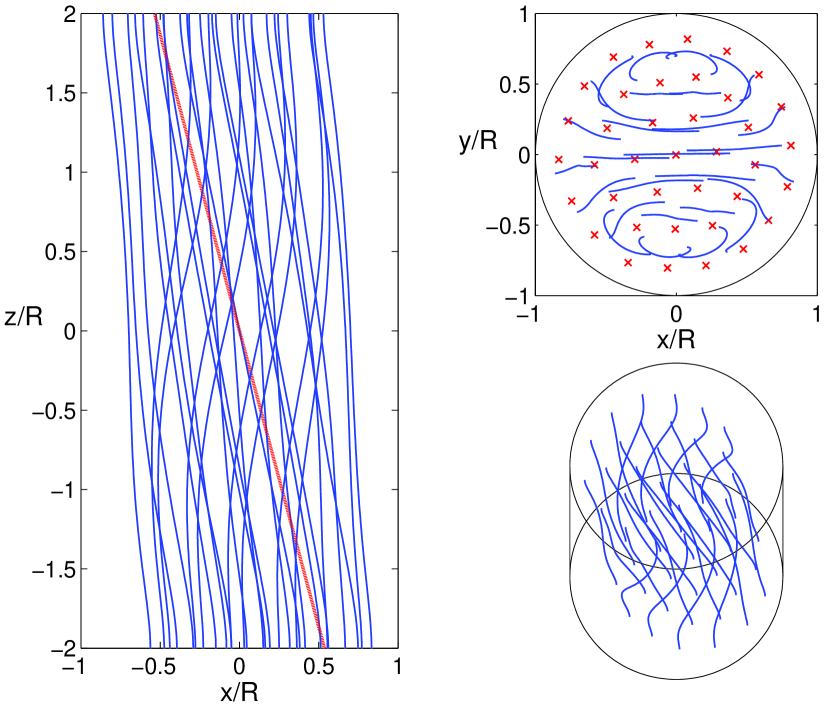
Figure 6: (Color online) Stable vortex array configuration, when $\Omega=50$ mrad/s in a cylinder with $L=4R=12$ mm and a tilt angle of 15 degrees. Left: Side view along the $y$-axis where the red straight line denotes the rotation axis. Top right: Top view where the crosses denote the equilibrium location of straight vortices at zero tilt, the configuration used as an initial guess for the calculations.. Bottom right: Perspective view of the same configuration. During the iteration 10 out of the 38 initial vortices annihilate, which indicates that the counterflow at the cylindrical boundary needs to be large enough to prevent the vortices that terminate to the outer boundary from shrinking away. The calculations were done using mutual friction parameters that correspond to $T=0.8T_{\rm c}$ for ³He-B. A similar configuration can be obtained at lower temperatures where it only takes much longer time to reach equilibrium, owing to much smaller mutual friction. Numerical resolution is characterized by $h_{\rm min}$ = 0.04 mm and $h_{\rm max}$ = 0.25 mm.

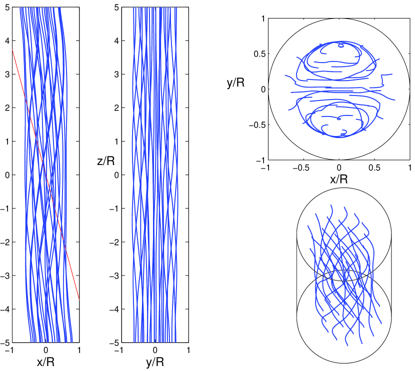
Figure 7: (Color online) Stable vortex array configuration, when $\Omega=50$ mrad/s in a cylinder with $L=10R=30$ mm and a tilt angle of 15 degrees. Left: Side view along the $y$-axis where the red straight line denotes the rotation axis. Center: Side view along the $x$-axis. Top right: Top view. Bottom right: Perspective view of the same configuration. During the iteration 15 out of the 38 initial vortices annihilate. The calculations were done using mutual friction parameters that correspond to $T=0.8T_{\rm c}$ in ³He-B. The initial configuration and the numerical resolution were the same as in Fig. 6.

For small rotation velocities and small tilt angles one may observe a static steady state. This state is most likely not the absolute energy minimum. Frequently the calculations for straight vortices have shown that different initial configurations will lead to metastable states with very similar energiesfetterSurf . Some of these steady states in the tilted cylinder are shown in Figs. 6 and 7. These configurations were obtained from an initial array of straight vortices along the cylinder axis as the starting state and then iterating the equation of motion with a given tilt angle. As in the single vortex case, one may notice that in a long cylinder the resulting vortex bundle is oriented more along the cylinder axis than along the rotation axis. Additionally, the vortices become slightly twisted, which results from the tendency to reduce the axial counterflow. This twist cannot be seen in the case of a single vortex, since the vortex lies in the plane where the axial flow is absent.

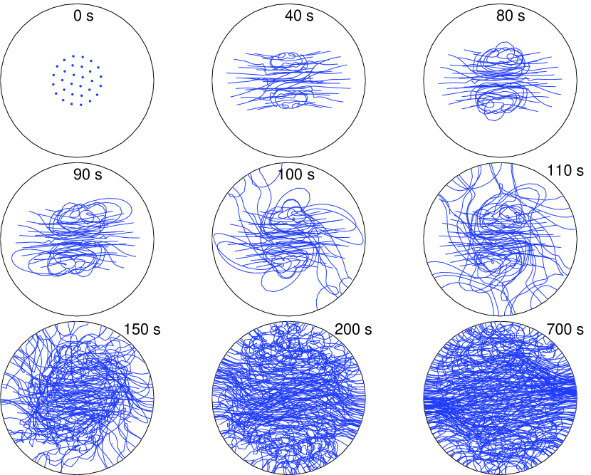
Figure 8: (Color online) Development of the dynamic steady state, when $L$ = $6R$ = 18 mm for a rotation velocity of 250 mrad/s and a tilt angle of 30 degrees. The mutual friction parameters correspond to $T=0.4T_{c}$ in $\textthreesuperior$He-B. The initial configuration is an array of 30 rectilinear vortices that become unstable due to the Glaberson instability. Similar break-up of the vortex array can also be seen in simulations done at $T=0.8T_{c}$. Numerical resolution is characterized by $h_{\rm min}$ = 0.10 mm and $h_{\rm max}$ = 0.30 mm. See also Fig. 9.

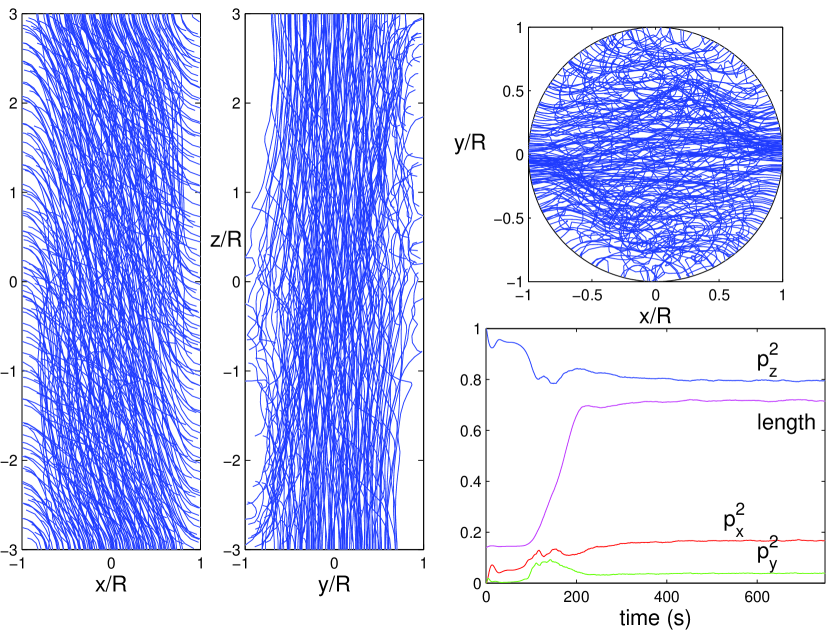
Figure 9: (Color online) Structure of the tangled bundle of vortices at 750 s in more detail for simulations with $L$ = $6R$ = 18 mm at a rotation velocity of 250 mrad/s and a tilt angle of 30 degrees. The mutual friction parameters correspond to $T=0.4T_{c}$ in $\textthreesuperior$He-B. Left: View along the $y$-axis that is perpendicular to the plane defined by the rotation and cylinder axes. Center: View along the $x$-axis. Top right: Top view along the cylinder axis. Bottom right: Time development of the polarization $p_{i}^{2}=\int(\hat{\bf s}^{\prime}\cdot\hat{\bf i})^{2}d\xi/\int d\xi$ and the total length ${\cal L}=\int d\xi$ of the vortex tangle. This length ${\cal L}$ is scaled by the combined total length of rectilinear vortices in an array at zero tilt, in the continuum approximation that is $(2\Omega/\kappa)\pi{R}^{2}L$.

With large enough tilt and rotation velocity the initial array of straight vortices suffers the Glaberson instability, as described above for an infinitely long cylinder. Our simulations show that the equation for the critical number of vortices, Eq. (11), gives an estimate of the instability also in a cylinder of finite length. If the number of vortices exceeds this value, then at the location of the largest axial flow the vortices go unstable. This is illustrated in Fig. 8 where the simulations were started with 30 straight vortices at the center of the cylinder. The configuration at 750s is shown in Fig. 9, together with the time development of vortex length and average polarization, $p_{i}^{2}=\int(\hat{\bf s}^{\prime}\cdot\hat{\bf i})^{2}d\xi/\int d\xi$. The initial vortex array, which has the polarization $p_{z}^{2}=1$ and $p_{x}^{2}=p_{y}^{2}=0$, is broken by the Glaberson instability. This has the result that the polarization along the $z$-axis decreases at the same time as the vortex length increases. The final steady state value for $p_{z}^{2}=0.80$ is higher than what would result if all the vortices would be along the rotation axis, in which case $p_{z}^{2}=\cos^{2}\eta=0.75$ (and $p_{x}^{2}=\sin^{2}\eta=0.25$). Since the turbulent fluctuations (Kelvin waves along vortices) and also the bending of vortices towards the radial direction near $\rho=R$ tend to decrease the polarization along the $z$-axis one may safely argue that even in this dynamical steady state there is a tendency of the vortices to orient themselves along the symmetry axis of the cylinder.

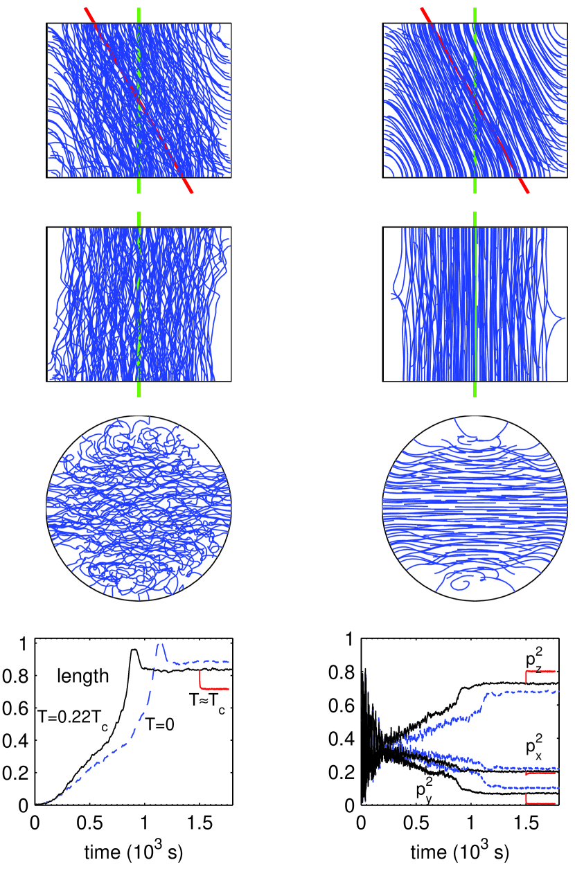
Figure 10: (Color online) Comparison between the low and high temperature vortex configurations for a short cylinder when $L$ = 5 mm, $R$ = 3 mm, $\Omega$ = 0.25 rad/s and $\eta$ = 30^∘. Now the vortices are mostly along the rotation axis (noted by the red line in the uppermost plots). From top to bottom these three different views correspond to a view along the $y$-, $x$-, and $z$-axis, respectively. The low temperature configuration (taken at $t$ = 1800 s) on the left is for $T=0.22T_{c}$ in ³He-B and was obtained by using a single vortex, a quarter ring, as an initial configuration. The high temperature configuration on the right, which corresponds to mutual friction parameters $\alpha$ = 10 and $\alpha^{\prime}$ = 0.9, was obtained by using the configuration at $t$ = 1500 s from the simulations at $T=0.22T_{c}$ as an initial guess and iterating for 262 seconds. Bottom left: Time development of the total vortex length, scaled by $(2\Omega/\kappa)\pi{R}^{2}L$. The solid black line corresponds to $T=0.22T_{c}$ and the solid red line, which starts at $t$= 1500 s, is the high temperature limit. The dashed blue line is a zero temperature calculation where we have set $\alpha=\alpha^{\prime}=0$ and the only dissipation is due to numerics. The initial configuration for the $T\rightarrow 0$ calculation was the same as for $T=0.22T_{c}$. Bottom right: Time development of the polarization of the vortex tangle. Color-coding is the same as for the vortex length. Large oscillations at small times result from the motion of a single (or few) vortex around the cylinder.

A somewhat surprising result from this simulation (and some other similar ones which we have performed at somewhat different temperature or with different $L$) is that after the instability it is difficult to obtain a static steady state, which presumably would be the thermodynamic equilibrium configuration. Even after the vortex length and polarization of the vortex tangle have settled to a steady state value one may still observe creation of new vortices in regions of high axial counterflow (which arises from the potential flow) owing to the Glaberson instability and a reconnection with the cylinder boundary. These newly generated vortices are then driven towards less turbulent regions. At the same time there is continuous annihilation of small vortex loops near the cylinder ends in regions of small counterflow. It is possible that our simulations do not extend far enough in time and that a static solution follows at much later times. Another possibility is that the calculation gets stuck in a local energy minimum and a possible static solution at lower energy may not be found with this initial configuration of vortices. This would also mean that experimentally it might be possible to observe a similar dynamic state.

At high temperatures the vortices become smoother and the turbulent regions, that can be seen in Figs. 8 and 9 at $T=0.4T_{c}$, become much more damped, but surprisingly some dynamics may still remain. For example, Kelvin waves are still created in the regions of largest axial flow. Similarly some vortices shrink in the regions of small counterflow near the cylinder ends. A comparison between the low and high temperature states is shown in Fig. 10. The low temperature state at $T=0.22T_{c}$ was obtained from an initial unstable configuration with single vortex in the form of a quarter ring starting from the bottom of the cylinder and bending to the outer wall. At low temperatures with a tilt angle of 30^∘ this configuration is unstable, leading to the creation of new vortices via reconnection at the boundary. At high temperatures the same initial configuration does not lead to vortex multiplication. Therefore the high temperature state, which here corresponds to $T\approx T_{c}$ (using $\alpha=10$ and $\alpha^{\prime}=0.9$), was obtained using the state from the $T=0.22T_{c}$ calculation at $t$=1500 s as initial configuration and iterating the vortex motion with high mutual friction. The steady state which was obtained this way was still a dynamical one after 300s of evolution, but the creation and annihilation of vortices was a quite regular process. This can be seen, for example, by investigating the vortex length, which shows small fluctuations but also clear oscillations with a periodicity of order 10 seconds. Fig. 10 shows also that the steady state vortex length increases and the axial polarization decreases with decreasing temperatures. This is due to fluctuations (Kelvin waves) on the vortices which are suppressed at high temperatures. The difference in steady state vortex length between the low and high temperature states is of order 20%. In reality the difference is larger since simulations cannot describe structures that are smaller than the numerical resolution, which in these runs is determined by $h_{\rm min}$ = 0.10 mm and $h_{\rm max}$ = 0.30 mm. A small overshoot in vortex length, that can be seen in simulations at low temperatures before the length saturates, indicates that a surplus of vortices is created before the final steady state is reached. Further analysis of the present simulations and more calculations are required to understand the complex dynamic phenomena in a tilted cylinder at large tilt angles with a large number of vortices. For example, the verification of Eqs. (10) and (11) is far from complete, especially when $\Omega_{\rm c}$ (or equally when $N_{\rm c}$) is large. Unfortunately the simulations take a lot of time and to determine whether the steady state is static or dynamical one is a tedious task.

V Conclusions

We have investigated vortex motions in a rotating cylinder where the rotation axis is not parallel to the symmetry axis of the cylinder. We have determined the steady state solutions and obtained that for small tilt angles the stable configuration consists of vortices that are along the cylinder axis, rather than the rotation axis. Therefore the assumptions behind the previously calculated resultmathieu might be inappropriate although there the calculations concerned a different flow geometry. For large tilt angles (but still well below 90^∘) the steady state solution, especially at low temperatures, may be a dynamical one, which would make it possible to study a polarized turbulence in a well controlled environment, especially in superfluid ³He-B where strong vortex pinning can be ignored. Since the vortex configuration is different from the expected one, it might be appropriate to reconsider the idea of a tilt-dependent mutual friction parameter, $B(\eta)$, as used in Ref. mathieu to interpret second-sound measurements in superfluid ⁴He. However, one should note that in He-II pinning is important and might alter the results.

- (1) D. Stauffer and A.L. Fetter, Phys. Rev. 168, 156 (1968).
- (2) J.A. Northby and R.J. Donnelly, Phys. Rev. Lett. 25, 214 (1970).
- (3) V.M. Ruutu, J.J. Ruohio, M.Krusius, B. Plaçais, and E.B. Sonin, Physica B 255, 27 (1998).
- (4) A.P. Finne, V.B. Eltsov, G. Eska, R. Hänninen, J. Kopu, M. Krusius, E. V. Thuneberg, and M. Tsubota, Phys. Rev. Lett. 96, 085301 (2006).
- (5) P. Mathieu, B. Plaçais, and Y. Simon, Phys. Rev. B 29, 2489 (1984).
- (6) M. Kobayashi and M. Tsubota, Phys. Rev. A 76, 045603 (2007); J. Low Temp. Phys. 150, 587 (2008).
- (7) L.M. Milne-Thomson, Theoretical Hydrodynamics 5th ed. (Macmillan, New York, 1968).
- (8) L.D. Landau and E.M. Lifshitz, Fluid Mechanics (Pergamon Press, Oxford, 1963).
- (9) V.B. Eltsov, R. de Graaf, R. Hänninen, M. Krusius, R.E. Solntsev, V.S. L’vov, A.I. Golov, and P.M. Walmsley, in Progress in Low Temperature Physics: Quantum Turbulence, Vol. 16, 45-146 (2009);
- (10) V.M.H. Ruutu, Ü. Parts, J.H. Koivuniemi, N.B. Kopnin, and M. Krusius, J. Low Temp. Phys. 107, 93 (1997).
- (11) K.W. Schwarz, Phys. Rev. B 31, 5782 (1985).
- (12) K.W. Schwarz, Phys. Rev. B 38, 2398 (1988).
- (13) T.D.C. Bevan, A.J. Manninen, J.B. Cook, H. Alles, J.R. Hook, and H.E. Hall, J. Low Temp. Phys. 109, 423 (1997).
- (14) T.D.C. Bevan, A.J. Manninen, J.B. Cook, A.J. Armstrong, J.R. Hook, and H.E. Hall, Phys. Rev. Lett. 74, 750 (1995).
- (15) E.B. Sonin, Rev. Mod. Phys. 59, 87 (1987).
- (16) A.P. Finne, T. Araki, R. Blaauwgeers, V.B. Eltsov, N.B. Kopnin, M. Krusius, L. Skrbek, M. Tsubota, and G.E. Volovik, Nature 424, 1022 (2003).
- (17) M. Tsubota, C.F. Barenghi, T. Araki, and A. Mitani, Phys. Rev. B 69, 134515 (2004).
- (18) M. Tsubota, T. Araki, and C.F. Barenghi, Phys. Rev. Lett. 90, 205301 (2003).
- (19) V.B. Eltsov, A.P. Finne, R. Hänninen, J. Kopu, M. Krusius, M. Tsubota, and E. V. Thuneberg, Phys. Rev. Lett. 96, 215302 (2006).
- (20) R.J. Zieve and L.A.K. Donev, J. Low Temp. Phys 121, 199 (2000).
- (21) R. Hänninen, A. Mitani, and M. Tsubota, J. Low Temp. Phys. 138, 589 (2005).
- (22) V.B. Eltsov, A.I. Golov, R. de Graaf, R. Hänninen, M. Krusius, V.S. L’vov, and R.E. Solntsev, Phys. Rev. Lett. 99, 265301 (2007).
- (23) W.I. Glaberson, W.W. Johnson, and R.M. Ostermeier, Phys. Rev. Lett. 33, 1197 (1974); R.M. Ostermeier and W.I. Glaberson, J. Low Temp. Phys. 21, 191 (1975).
- (24) R.J. Donnelly, Quantized Vortices in Helium II (Cambridge University Press, Cambridge, UK, 1991).