Manipulation of double-dot spin qubit by continuous noisy measurement

Abstract

We consider evolution of a double quantum dot (DQD) two-electron spin qubit which is continuously weakly measured with a linear charge detector (quantum point contact). Since the interaction between the spins of two electrons depends on their charge state, the charge measurement affects the state of two spins, and induces non-trivial spin dynamics. We consider the regimes of strong and weak coupling to the detector, and investigate the measurement-induced spin dynamics both analytically and numerically. We observe emergence of the negative-result evolution and the system stabilization due to an analog of quantum Zeno effect. Moreover, unitary evolution between the triplet and a singlet state is induced by the negative-result measurement. We demonstrate that these effects exist for both strong and weak coupling between the detector and the DQD system.

I Introduction

Quantum dots (QDs) recently have attracted much attention as very suitable candidates for studying evolution of a single quantum system. Moreover, QDs are very promising candidates for quantum information processing. An electron spin in a quantum dot is a good representation for a qubit, being a natural two-state quantum system. Manipulations of the single QDs and double-QD (DQD) systems can be achieved using external magnetic fields and gate voltages HansonReview , which implement injection of an electron (or pair of electrons for DQD) in a given spin state, or some unitary rotation in a two-spin space. However, it is not easy to achieve the full set of transformations in the Hilbert space of two coupled spins QDman1 ; QDman2 ; QDman3 ; QDman4 : some transformations require a strong gradient of magnetic fields on a nanometer scale, and advanced techniques are needed for performing spin rotations rapidly and reliably.

Thus, it is interesting to explore other possible ways of manipulating electron spins in DQD structures. In particular, it is natural to study whether measurement of the charge state of the DQD may help drive the desired evolution of the two-spin system. The weak continuous measurement Dalibard ; Carmichael ; WisemanMilburn ; Kor-99-01 , which monitors the system in question, and therefore affects its evolution, may provide an additional and useful tool for controlling the electron spins in DQD systems. At some level of description of a probed quantum system plus detector, it is postulated that the fundamental measurement process consists of direct particle detections (e.g., photons, electrons, etc.) or absence of any detection. The absence of a detection for specific time interval constitutes a negative result. In both cases (“detection” or “no detection”) the quantum state of the system evolves according to the provided information and the evolution can be described using quantum Bayesian inference.Kor-99-01 E.g., for a two-level atom which did not decay by time $t$ the evolution of the atom’s density matrix takes the form:

$$\rho_{ee}(t)=\frac{\rho_{ee}(0)\,e^{-\Gamma_{sp}t}}{\cal N},\ \rho_{gg}(t)=\frac{\rho_{gg}(0)}{\cal N}\ \$$ (1)

$$|\rho_{eg}(t)|=|\rho_{eg}(0)|\,\sqrt{\frac{\rho_{ee}(t)\,\rho_{gg}(t)}{\rho_{ee}(0)\,\rho_{gg}(0)}},\qquad$$ (2)

where $e^{-\Gamma_{sp}t}$ is the conditional probability not to decay from the excited state $|e\rangle$ (ground state $|g\rangle$ is supposed stable), $\Gamma_{sp}$ is the spontaneous decay rate, and ${\cal N}\equiv\rho_{gg}(0)+\rho_{ee}(0)\,e^{-\Gamma_{sp}t}$. The classical Bayesian update of the diagonal elements, Eq.(1), reflects an information-related evolution. Also, Eq.(2) shows that the coherence ratio $|\rho_{eg}|/\sqrt{\rho_{ee}\,\rho_{gg}}$ is conserved; in particular, a pure state remains pure.

The above evolution has been proposed and discussed mainly in the context of quantum optics. Epstein-Dicke ^,Dalibard ; Carmichael ; WisemanMilburn For solid state systems, it has been realized recently, using an artificial two-level system: a superconducting “phase” qubit, measured via tunneling of its superconducting phase.Katz-Sci The detection of tunneling was considered as an instantaneous processKatz-Sci ; Pryadko in the highly non-linear detector (dc-SQUID) that implies detector relaxation rates much faster than the qubit “decay rate”.

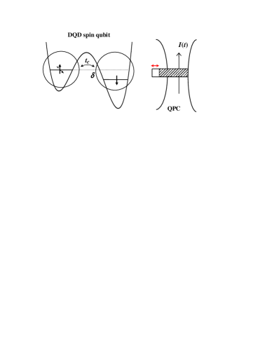
Figure 1: Schematic of a DQD spin system measured by a QPC; the QPC current $I(t)$ is affected by the charge state of the DQD. In quantum Zeno regime the tunneling between dots is suppressed while the spin qubit undergoes continuous negative-result evolution.

In this paper we consider another realization of a solid state qubit and a linear detector measuring continuously. Nevertheless, it can behave similarly to the above examples in certain measurement regimes. We will consider a semiconductor double quantum dot (DQD) spin system (Fig.1) where two electrons can be in either of the dots and the relevant states are spin-charge states.LossDiVi ; Kouwenhoven-Nat1 ; Marcus-Sci ; HansonReview At relatively small time scales (from ns to $\mu$s) the electron tunneling between the dots preserves the system’s total spin that allows spin-selective evolution and leads to the so called spin-to-charge conversion.HansonReview This allows the measurement of the DQD spin system by a charge sensitive detector such as a quantum point contact (QPC)Kouw-prl94 ; Marcus-Sci or single electron transistor (SET).Rimberg-nat

For our system (Fig.1) the spin qubitMarcus-Sci is formed by the singlet spin state $|S(1,1)\rangle$ and the triplet state $|T_{0}(1,1)\rangle$ that has a zero spin projection on an external magnetic field (here, e.g., $(1,1)$ denotes a charge state when one electron is in the left dot and the other is in the right dot). Spin conservation allows transition between the singlet $|S(1,1)\rangle$ and the localized singlet, $|S(0,2)\rangle$, while a transition from the triplet state is spin-blocked. Thus, the state $|S(0,2)\rangle$ can be used for preparation and subsequent measurement of the spin qubit. For a weak measurement the system-detector coupling $\Gamma$ is finite and defines the time scale of measurement evolution (in particular, $1/\Gamma$ is of the order of the time needed to distinguish the two different charge states by the QPC). The spin system evolution will be an interplay of the non-unitary dynamics due to measurement and the dynamics associated with the system’s internal Hamiltonian.

The purpose of this work is to develop the theory of quantum evolution of a DQD two-electron spin system under the continuous measurement by a linear charge detector such as a QPC that is based on the Bayesian approach.Kor-99-01 ; Kor-osc ; Ruskov-neg Initially motivated by experimentMarcus-Sci we pose the question: “How the measurement by a QPC will affect the spin qubit state and is it possible to use continuous measurement for manipulation of the quantum state ?” The system state is continuously updated according to a given measurement record due to quantum back action.Kor-99-01 On typical system’s times when many electrons pass through the QPC, the quantum evolution is conditioned on the fluctuating detector current $I(t)$.

We identify regimes when the system-detector coupling becomes large relative to a typical system frequency, that leads to suppression of coherent tunneling transitions. The associated stabilization of the states in continuous measurement (see, e.g., Ref.Kor-osc ; RusKor-ent ; Ruskov-Zeno ) is an analog of the well known quantum Zeno effect.Khalfin ; MisraSudarshan ; Peres Since the system-detector coupling is finite, the Zeno stabilization does not last forever. The stabilized states switch to each other with a rate $\Gamma_{sw}\ll\Gamma$. The switching happens on a time scale $1/\Gamma$. In fact, on this time scale the switching transition becomes irreversible. For an ensemble averaged description of the state evolution we will show that the irreversibility corresponds to an exponential decay (compare with Ref.Pryadko ) with the decay rate $\Gamma_{sw}$.

Correspondingly, in the case of a spin qubit we show via numerical simulation of the measurement process that the switching rate $\Gamma_{sw}$ plays the role of the spontaneous decay rate $\Gamma_{sp}$ for the two-level atom described above. Despite the quantum back action noise reflecting the noisy output, the spin qubit state will evolve according to Eqs.(1), (2) in a spin-charge basis that corresponds to the Zeno stabilized states. In particular, in our analysis the negative-result evolution of the qubit subsystem is not postulated but emerges from continuous noisy measurement evolution and Hamiltonian evolution at a microscopic level.

The paper is organized as follows. In Sec. II we review/derive the Bayesian equations for weak continuous measurement of a DQD two-electron spin system. In Sec.  III we investigate the measurement collapse scenarios for different coupling regimes and give qualitative and quantitative explanations of the obtained results. In Sec.  IV we estimate the detector-system coupling and other important parameters that could be relevant for an experiment to confirm our results. We also comment on the role of various sources of decoherence.

II DQD two electron system and measurement device

II.1 Hamiltonian and time scales

The system of two electrons confined in the DQD, and the quantum point contact as a charge sensing detector are shown in Fig.1. External gate voltages form the potential profile of the DQD and are well controlled in the experiment.HansonReview In particular, changing the energy difference between the dots, $\delta$, allows continuous tuning of the charge configuration between $(1,1)$ and $(0,2)$: when the electrons are in the right dot $(0,2)$ the ground state is the spin singlet $|S(0,2)\rangle$. The interdot tunneling coupling $\Omega$ allows coherent transitions between the singlet spin-charge states $|S(1,1)\rangle$ and $|S(0,2)\rangle$ which are close in energy (for $\delta=0$, the states $|S(1,1)\rangle$ and $|S(0,2)\rangle$ are in resonance). Transitions between the triplet states $|T(1,1)\rangle$ and $|T(0,2)\rangle$ are suppressed due to large energy mismatch: the highly energetic triplet states $|T_{\pm,0}(0,2)\rangle$ are well separated in energy from the singlet $|S(0,2)\rangle$Taylor ($\Delta E_{ST}\sim 400\mu eV$) due to tight confinement and on site exchange interaction. In the $(1,1)$ configuration the spin qubit subspace is formed by the singlet $|S(1,1)\rangle$ and the triplet state $|T_{0}(1,1)\rangle$ with zero spin projection on an external magnetic field $B$; the applied field removes the triplet degeneracy by splitting off the $|T_{\pm}(1,1)\rangle$ states (splitting $\Delta_{\pm}\approx 2.5\mu\mbox{eV}$ for the GaAs DQD described in Ref.Marcus-Sci ). Thus, the DQD spin system is considered below as a three state quantum system (qutrit).

Introducing the short notations for the relevant three states: $|1\rangle\equiv|S(0,2)\rangle$, $|2\rangle\equiv|S(1,1)\rangle$, $|3\rangle\equiv|T_{0}(1,1)\rangle$, we write the system hamiltonianJouravlevNazarov ; Taylor :

$${\cal H}_{DQD}=-\delta\ |1\rangle\langle 1|+\frac{\Omega}{2}\ (|1\rangle\langle 2|+|2\rangle\langle 1|)$$

$$+\varepsilon_{S}\ |2\rangle\langle 2|+\varepsilon_{T}\ |3\rangle\langle 3|.$$ (3)

The presence of the $|T_{\pm,0}(0,2)\rangle$ states induces small exchange energies $\varepsilon_{S}$, $\varepsilon_{T}$ which can be taken into account perturbatively;Taylor in what follows we will neglect these energies that are of the order of $\Omega^{2}/\Delta E_{ST}\ll\Omega$. Other possible terms in the Hamiltonian ${\cal H}_{DQD}$ (that are present for a general qutrit systemCavesMilburn ) are suppressed due to conservation of spin.

In the total Hamiltonian of system plus detector

$${\cal H}={\cal H}_{DQD}+{\cal H}_{det}+{\cal H}_{int},$$ (4)

the (low transparency) QPC detector Gurvitz is described with

$${\cal H}_{det}=\sum_{l}E_{l}c_{l}^{\dagger}c_{l}+\sum_{u}E_{u}c_{u}^{\dagger}c_{u}+\sum_{l,u}(Tc_{u}^{\dagger}c_{l}+\mbox{H.c.});$$ (5)

here the operator $c^{\dagger}_{l}$ ($c^{\dagger}_{u}$) creates an electron in the lower (upper) lead of the detector (Fig.1) and the tunneling $T$ between leads is assumed energy independent.

The system–detector interaction can be written in analogy with the qubit case; for a general qutrit measured by a hypothetical detector that can distinguish all three states one formally writes the interaction Hamiltonian as proportional to the two [$SU(3)$] generators, that are diagonal in the spin-charge basis:

$${\cal H}_{int}=\sum_{l,r}\left[A\,(|1\rangle\langle 1|-|2\rangle\langle 2|)\otimes c_{u}^{\dagger}c_{l}\right.$$

$$\left.+B\,(|1\rangle\langle 1|+|2\rangle\langle 2|-2\,|3\rangle\langle 3|)\otimes c_{u}^{\dagger}c_{l}+\mbox{H.c.}\right].$$ (6)

Introducing detector transmission probability $T_{k}$ for each system state $|k\rangle$, the average currents can be expressed as $I_{k}=2\pi T_{k}\rho_{l}\rho_{u}e^{2}V/\hbar,\ k=1,2,3$, where $V$ is the detector bias voltage, and $\rho_{l}$ and $\rho_{u}$ are the densities of states in the lower and upper lead. In the case of QPC, which cannot distinguish between states $|2\rangle\equiv|S(1,1)\rangle$ and $|3\rangle\equiv|T_{0}(1,1)\rangle$ the tunneling amplitudes $A$ and $B$ are not independent: $T_{2}=|T-A+B|^{2}=T_{3}=|T-2B|^{2}$, since the corresponding average currents are equal, $I_{2}=I_{3}\equiv I_{(1,1)}$. For the state $|1\rangle\equiv|S(0,2)\rangle$ the average current $I_{(0,2)}\neq I_{(1,1)}$ and it can be distinguished from the $(1,1)$ states.

In what follows we consider a situation when the internal detector dynamics given by Eqs.(5), (6) is much faster than the two-spin dynamics due to ${\cal H}_{DQD}$. Also, it is assumed that the voltage applied to detector is large so that a typical detector decoherence time is much smaller than the typical electron tunneling times; thus, $\hbar/eV\ll e/I_{(0,2)},e/I_{(1,1)}\ll 1/\Omega$. The first inequality implies that coherences between different electron passages in the QPC can be neglected. Thus, the QPC detector will behave essentially classically on the typical time scale of the DQD two-spin dynamics.

II.2 Continuous quantum evolution according to the result

The quantum state evolution of an open quantum systemCarmichael ; Davies has an analog in a classical state estimation procedure;Holevo it takes into account the actual measurement record that is imperfectly correlated with the system state. In a situation when the QPC is a weakly responding detector, $|\Delta I|\equiv|I_{(0,2)}-I_{(1,1)}|\ll I_{(0,2)},I_{(1,1)}$, when every tunneling electron brings a little information about the system state, it is reasonable to condition the system evolution on the quasicontinuous noisy detector current $I(t)$.Kor-99-01 Typical measurement time (that reflects accumulation of a signal-to-noise ratio of order one) can be introducedShnirman ^,Kor-99-01 , $\tau_{meas}=2S_{0}/(\Delta I)^{2}\sim 1/\Gamma$, where $S_{0}\simeq 2eI_{(1,1)}$ is the low-frequency spectral density of the detector shot noise. [We have neglected small differences between shot noises.] The finite measurement time implies that given the noisy current $I(t)$, the system state is updated gradually. Below we sketch the derivation of the measurement evolution equations for a qutrit related to the “informational” Bayesian approach.Kor-99-01 ; Kor-ent

For the measurement evolution alone, the most straightforward way is to consider the elementary act of scattering of an incoming electron, $|i\rangle$, off the QPC tunnel barrier that depends on the charge state of the system, $|k\rangle$. The scattered state is expressed as a linear transform of the initial state: $|f\rangle=\hat{S}_{k}|i\rangle$ where the scattering matrix is (see, e.g., Ref.AverinSukhorukov, )

$$\hat{S}_{k}=\left(\begin{array}[]{cc}r_{k}&t_{k}^{*}\\ t_{k}&-r_{k}^{*}\\ \end{array}\right),$$ (7)

and $r_{k}$, $t_{k}$ are the reflection and transmission amplitudes. Following Jordan and Korotkov,JordanKorotkov every tunneling electron can be mapped to an ancilla qubit, whose basis states are the scattering states: $|R\rangle$ for a reflected electron, and $|T\rangle$ for a transmitted electron. Scattering will entangle the states of the ancilla qubit and the qutrit. Then projective measurement on the ancilla will lead to POVM (positive operator-valued measure) measurement operatorsNielsenChuang of the form: $\hat{M}_{R}=\mbox{diag}\{r_{1},r_{2},r_{3}\}$ and $\hat{M}_{T}=\mbox{diag}\{t_{1},t_{2},t_{3}\}$ that satisfy the completeness condition $\hat{M}_{R}^{\dagger}\,\hat{M}_{R}+\hat{M}_{T}^{\dagger}\,\hat{M}_{T}=1$. The diagonal form of these operators in the qutrit basis (the spin-charge basis) follows from the diagonal form of the interaction Hamiltonian ${\cal H}_{int}$, Eq.(6). For collecting electrons in the upper lead, the count of an electron updates the qutrit density matrix according to a POVM formula $\hat{\rho}^{{}^{\prime}}=\hat{M}_{T}\hat{\rho}\hat{M}_{T}^{\dagger}/{\cal P}_{T}$ where ${\cal P}_{T}=\mbox{Tr}[\hat{M}_{T}^{\dagger}\,\hat{M}_{T}\hat{\rho}]=\sum_{k}\rho_{kk}T_{k}$ is the total probability to find an electron in the upper lead and $T_{k}=|t_{k}|^{2}$ are the transmission probabilities introduced in the previous section. If an electron was not counted a similar update takes place using the measurement operator $\hat{M}_{R}$ and the reflection probabilities, $1-T_{k}=|r_{k}|^{2}$. In the basis where $\hat{M}_{R,T}$ are diagonal these evolutions take the form of Bayesian updates.JordanKorotkov

The evolution rate of the system density matrix will be related to the rate of tunneling through the QPC. Introducing an average number $A\,\delta t$ of (independent) tunneling attempts per time $\delta t$, the average currentLandauer (given the system state $|k\rangle$) is then $I_{k}=eAT_{k}$. For times of the order of individual tunneling times, $\delta t\sim e/I_{k}$, we can consider a negative-result evolution of the qutrit density matrix. For the evolution of the diagonal elements in case of no tunneling we write:

$$\rho_{kk}(\delta t)=\rho_{kk}(0)\,(1-T_{k})^{A\,\delta t}/{Norm}.$$ (8)

($Norm$ is a proper normalization.) For a low transparency QPC, $T_{k}\ll 1$, the number of attempts is large, $A\,\delta t\sim 1/T_{k}\gg 1$ so that $(1-T_{k})^{A\,\delta t}\approx e^{-T_{k}A\,\delta t}=e^{-\frac{I_{k}}{e}\delta t}$. Thus, we obtain a negative-result evolution similar to Eq.(1) where the spontaneous decay rate $\Gamma_{sp}$ is replaced by the tunneling rates $\frac{I_{k}}{e}$, each for every $k=1,2,3$. The evolution of the non-diagonal elements can be shown to be of the form similar to Eq.(2).

The above evolution can be hardly observed, since for typical system times, $1/\Omega,1/\Gamma\gg e/I_{k}$, many electrons pass through QPC. For $N$ independent attempts one can derive the conditional probability for $m$ successful tunnelingsJordanKorotkov (per time $\tau$) given the system is in state $|k\rangle$

$${\cal P}(m,N|k)=C_{N}^{m}T_{k}^{m}(1-T_{k})^{N-m},$$ (9)

so that the Bayesian update of the system (qutrit) density matrix can be shown to be of the form: $\rho_{kk}^{{}^{\prime}}=\rho_{kk}{\cal P}(m,N|k)/Norm$ and $\rho_{kl}^{{}^{\prime}}=\rho_{kl}\sqrt{\rho_{kk}^{{}^{\prime}}\rho_{ll}^{{}^{\prime}}/\rho_{kk}\rho_{ll}}$.

We mention that the update related to Eq.(9), is just a simple composition of $N$ elementary updates, each corresponding to tunneling $(1)$ or no tunneling $(0)$ of a single electron: e.g., for a result $\tilde{Q}=(0,1,\ldots,0)$ the measurement operator $\hat{M}_{\tilde{Q}}$ is just a multiplication of $N$ diagonal operators, $\hat{M}_{\tilde{Q}}=\hat{M}_{R_{1}}\hat{M}_{T_{2}}\ldots\hat{M}_{R_{N}}$. Also note that Eq.(9) sums up over $C_{N}^{m}$ identical possibilities since QPC cannot distinguish different sequences $\tilde{Q}_{1},\tilde{Q}_{2},\ldots$ with the same total charge tunneled to the right lead. By representing the (random) number $m$ of tunneling electrons per time interval $\tau$ through the QPC current, $m\equiv\tau\bar{I}(t,\tau)=\int_{t}^{t+\tau}I(t^{\prime})dt^{\prime}$, and using De Moivre-Laplace limit theorem ($N\gg 1$, $T_{k}$ fixed) we can replace ${\cal P}(m,N|k)$ by a Gaussian distribution for the measurement result $\bar{I}(t,\tau)$, given the state $|k\rangle$: $P_{k}(\bar{I})=\sqrt{\tau/\pi S_{0}}\exp{[-(\bar{I}(t,\tau)-I_{k})^{2}\tau/S_{0}]}$, where $I_{k}\simeq eMT_{k}/\tau$ is the average current, and $S_{0}$ is the shot noise spectral density for a low transparency and weakly responding QPC. The update of the system density matrix can be written again as a Bayesian (informational) evolution:Kor-99-01

$$\rho_{kl}(t+\tau)=\rho_{kl}(t)\frac{\sqrt{P_{k}(\bar{I})}\,\sqrt{P_{l}(\bar{I})}}{P(\bar{I})},$$ (10)

with the total probability of a particular result $\bar{I}$ given by $P(\bar{I})=\sum_{k}\rho_{kk}(t)P_{k}(\bar{I})$.

Differentiating Eq.(10) over $\tau$ (at $\tau\to 0$) one obtains a stochastic equation for the qutrit state evolution (in Stratonovich formOksendal ). Taking into consideration the (internal) Hamiltonian evolution and possible dephasing, one can write:

$$\dot{\rho}_{kl}=\frac{\rho_{kl}}{S_{0}}\sum_{j}\rho_{jj}\,\left\{(I_{k}-I_{j})\left(I(t)-\frac{I_{k}+I_{j}}{2}\right)\right.$$

$$\left.\qquad\ {}+(I_{l}-I_{j})\left(I(t)-\frac{I_{l}+I_{j}}{2}\right)\right\}$$

$$\qquad\ {}-\frac{i}{\hbar}[{\cal H}_{DQD},\rho]_{kl}-\gamma_{kl}\,\rho_{kl}.$$ (11)

Here $I(t)$ is the formal limit (at $\tau\to 0$) of the observed detector signal $\bar{I}(t,\tau)$. For numerical simulations of a measurement one complementsKor-99-01 Eq.(11) by

$$I(t)=\sum_{k}\rho_{kk}(t)I_{k}+\xi(t)$$ (12)

that is consistent with the statistics of $P(\bar{I})$; here $\xi(t)$ is a white noise with a spectral density $S_{\xi}=S_{0}$. Eq.(11) is of the same form as an analogous evolution equation for a system of $N$ qubits;Kor-ent here the summation is over the three qutrit states. The dephasing rates, $\gamma_{kl}$, are related to the detector non-ideality;Kor-99-01 ; back-action experimentallyBuks and theoreticallyKor-99-01 ; back-action ; AverinSukhorukov a QPC is close to an ideal detector. An SET is usually highly non-idealKor-99-01 , however it may reach ideality close to 1 in the co-tunneling or Cooper pair tunneling regime.cotun

It is worthwhile to note that the measurement evolution and the Hamiltonian evolution enter in Eq.(11) independently; they just reflect the measurement (POVM) and unitary postulates applied to the system at a coarse grained time $t\gg e/I_{k}\gg\hbar/eV$ where the evolution is noisy and quasicontinuous. In Sec. III we will show via numerical solutions of Eq.(11) that the continuous measurement evolution and the Hamiltonian evolution interplay non-trivially so that new effective (negative-result) measurement and Hamiltonian evolutions of the system arise at a larger time scale.

II.3 Ensemble averaged evolution of the system

A total ignorance of a particular measurement result $\bar{I}(t)$ corresponds to a situation when the QPC detector is considered just as a part of a (Markovian) environment surrounding the system. Correspondingly, the density matrix available to such an observer (denoted as $\langle\rho_{kl}\rangle$) will be quite different from that described by Eq.(11). The density matrix $\langle\rho(t)\rangle$ can be related to $\rho(t)$, Eq.(11) by a formal procedure of an ensemble averaging over possible results $\bar{I}(t)$ at every time moment $t$, similar to the classical probabilities.Holevo The averaging can be performed (for a sufficiently small time interval $\tau$), e.g., by using the total probability of a particular result $\bar{I}$, given by $P(\bar{I})$ and then simply adding the Hamiltonian evolution. The result will be a standard master equationLeggett

$$\langle\dot{\rho}_{kl}\rangle=-\Gamma_{kl}\,\langle\rho_{kl}\rangle-\frac{i}{\hbar}[{\cal H}_{DQD},\langle\rho\rangle]_{kl}$$ (13)

with ensemble-averaged dephasing rates

$$\Gamma_{kl}=(I_{k}-I_{l})^{2}/4S_{0}+\gamma_{kl}.$$ (14)

For a quantum limited (ideal) detector, $\gamma_{kl}=0$, the dephasing rates produced due to averaging are just $(I_{k}-I_{l})^{2}/4S_{0}$ which is the minimum allowed by quantum mechanics.Kor-99-01 ; Kor-osc ; back-action ; Ruskov-Bell

The individual dephasings, $\gamma_{kl}\neq 0$, may be a consequence of partial ignorance of the measurement resultKor-99-01 and are parameterized by the detector ideality (efficiency) $\eta$ ($0\leq\eta\leq 1$): $\gamma_{kl}=(\eta^{-1}-1)\,(I_{k}-I_{l})^{2}/4S_{0}$, i.e., $\Gamma_{kl}=(I_{k}-I_{l})^{2}/4S_{0}\eta$. Other sources of decoherence of the DQD system will be discussed in Sec. IV.

III Emergence of negative-result evolution in the qubit subspace

When the unitary evolution of the three-state system is taken into account one has to explore the full Bayesian Eq.(11), which, as a rule, does not provide simple solutions. In what follows, using Eq.(11), we will perform numerical simulation of the measurement process for various regimes of the system-detector dynamics. The non-trivial interplay of the quantum dynamics can be seen if one compares the effects of measurement evolution alone vs. total evolution. The measurement alone tends to collapse the system (qutrit) in either the state $|1\rangle$ or to the qubit subspace $\{|2\rangle,|3\rangle\}$ leaving states $|2\rangle$ and $|3\rangle$ unresolved. However, adding the continuous coherent mixing of $|1\rangle$ and $|2\rangle$ by ${\cal H}_{DQD}$ leads to effective resolution of the states $|2\rangle$ and $|3\rangle$, so that a continuous collapse happens either to the state $|3\rangle$ or to the remaining spin-singlet subspace.

If the continuous collapse happens to the singlet subspace, at small coupling $\Gamma$ the system will perform quantum oscillations, that are weakly perturbed by the measurement. When the coupling becomes large the picture is qualitatively different: one reaches the regime of Zeno stabilization of the system’s singlet states. The latter is characterized by long time intervals when the QPC current is either $I_{(1,1)}$ or $I_{(0,2)}$, interupted by rare switching between them; the qutrit state is correspondingly $|2\rangle\equiv|S(1,1)\rangle$ or $|1\rangle\equiv|S(0,2)\rangle$. If the system was initially into the qubit subspace, the continuous collapse takes the form of a slow negative-result evolution of the qubit state until it eventually switches to $|S(0,2)\rangle$.

The negative-result evolution is a Bayesian evolution conditioned by the information that the “qubit did not switch”. This evolution emerges in the Zeno regime as a solution of the underlying Bayesian stochastic evolution, Eq.(11). It is important to note that the key feature for establishing a negative-result evolution is the irreversibility of the switching event (compare with Ref.Pryadko, ). Within the stochastic measurement evolution, the irreversibility is consistent with an important property of Eq.(11) that is seen in numerical simulations: given a measurement record $I(t)$, two evolutions that start from different initial states, $\rho^{(1)}(0)$ or $\rho^{(2)}(0)$, will become undistinguishableKor-99-01 ; Ruskov-Zeno at a time scale of the order or greater than $1/\Gamma$. In other words the system “forgets” its initial state, $\rho(0)$ so that further evolution is dominated by the result, $I(t)$ itself. The regime of current stabilization, (that is essentially classicalRuskov-Bell ) then would correspond to irreversibility of the switching event.

III.1 Collapse scenarios

For a numerical simulation of the measurement process we use Eq.(11), supplemented with the relation for the current signal, Eq.(12), where we incorporated the current level degeneracy for the states $|2\rangle$ and $|3\rangle$ ($I_{2}=I_{3}=I_{(1,1)}$). In order to understand the collapse scenarios it is instructive to look at the stochastic equation for the relevant density matrix elements transformed from Eq. (11) to their Itô formOksendal (below we use $\hbar=1$).

$$\dot{\rho}_{11}=-\Omega\,\mbox{Im}\rho_{12}+\rho_{11}\,(1-\rho_{11})\,\frac{\Delta I}{2S_{0}}\,\xi(t),\ \$$ (15)

$$\dot{\rho}_{33}=-\rho_{11}\rho_{33}\,\frac{2\Delta I}{S_{0}}\,\xi(t),$$ (16)

$\qquad\qquad\qquad\dot{\rho}_{22}=-\dot{\rho}_{11}-\dot{\rho}_{33}$, and

$$\dot{\rho}_{12}=i\,\delta\,\rho_{12}+i\,\frac{\Omega}{2}\,(\rho_{11}-\rho_{22})-\Gamma_{12}\,\rho_{12}$$

$$\qquad\ \ {}-(2\rho_{11}-1)\,\rho_{12}\,\frac{\Delta I}{S_{0}}\,\xi(t),$$ (17)

$$\dot{\rho}_{13}=i\,\delta\,\rho_{13}-i\,\frac{\Omega}{2}\,\rho_{23}-\Gamma_{13}\,\rho_{13}$$

$$\qquad\ \ {}-(2\rho_{11}-1)\,\rho_{13}\,\frac{\Delta I}{S_{0}}\,\xi(t),$$ (18)

$$\dot{\rho}_{23}=-i\,\frac{\Omega}{2}\,\rho_{13}-\rho_{11}\,\rho_{23}\,\frac{2\Delta I}{S_{0}}\,\xi(t).$$ (19)

Here $\Delta I\equiv I_{(0,2)}-I_{(1,1)}$ is the current difference between the charge subspaces that can be distinguished by the QPC. The system-detector coupling explicitly enters in Eqs.(17),(18) as $\Gamma_{12}=\Gamma_{13}\equiv(\Delta I)^{2}/4S_{0}+\gamma_{12}=\Gamma=(\Delta I)^{2}/4S_{0}\eta$

In the absence of the Hamiltonian, ${\cal H}_{DQD}=0$, the equation for $\rho_{11}$ becomes a pure noise and decouples; it can be heuristically considered as a (position dependent) Wiener process for the restricted variable $0\leq\rho_{11}\leq 1$ with a diffusion coefficient, $\sim\rho_{11}(1-\rho_{11})$, approaching a minimum (zero) at the endpoints, $\rho_{11}=0$ or $\rho_{11}=1$. Just as in the single qubit caseKorJordan-undo it suggests that the endpoints are the two possible attractors for a given realization of the measurement. In the qutrit case, the measurement also preserves the ratio $\rho_{22}/\rho_{33}\equiv\alpha$ and the measurement evolution happens on a ray $\rho_{33}=(1-\rho_{11})/(1+\alpha)$ in the physical triangle of the plane $(\rho_{11},\rho_{33})$ [$0\leq\rho_{kk}\leq 1,k=1,2,3$]. Switching on the Hamiltonian mixes the density matrix components leaving $\rho_{33}$ unaffected; geometrically this is represented as a horizontal moving in the plane $(\rho_{11},\rho_{33})$ that changes $\alpha$ [causing the system to change from one ray to another]. From this point of view it is easy to imagine how the new attractors become $\rho_{33}=0$ (a horizontal ray) or the point $\rho_{33}=1$. Finally, it is clear from Eq.(16) that if the system is in either of the subspaces, $\{|1\rangle,|2\rangle\}$ or $|3\rangle$, it will remain there: neither Hamiltonian nor measurement evolution mixes the subspaces, which is true for any DQD parameters, $\delta$, $\Omega$. The decoupling of subspaces is a consequence of the spin blockade and indistinguishability of the states $|2\rangle$ and $|3\rangle$ by measurement.

The decoupling implies that the system will continuously collapse to one of the subspaces under a weak continuous measurement as seen in numerical simulations, Fig.2. Since the corresponding ensemble averaged equation for $\rho_{33}(t)$ is simply $d\langle\rho_{33}(t)\rangle/dt=0$ (ensemble averaging implies just nullifying of the noise in Itô form of the equationsOksendal ), then the ensemble averaged density matrix element is conserved: $\langle\rho_{33}(t)\rangle=\rho_{33}(0)$. Thus, it must be that the fraction of members of the ensemble that collapses to $\rho_{33}(t)=1$ (after a sufficient measurement time $t$) is just $\rho_{33}(0)$, which means that the probability of collapse to either of the subspaces is $\rho_{33}(0)$ and $1-\rho_{33}(0)$ respectively (i.e., the usual probability rules apply).

III.2 System evolution at small coupling. Quantum oscillations and spin blockade

In order to characterize the emergence of a negative result evolution from continuous noisy measurement we will first consider the case when the system may establish quantum oscillations weakly perturbed by the measurement, i.e., when negative-result evolution is not yet established. In particular, this happens for small system-detector coupling, $\Gamma\ll\Omega$ while the quantum dots detuning $\delta$ is also small. For simplicity, we first consider the case of an ideal detector, $\eta=1$.

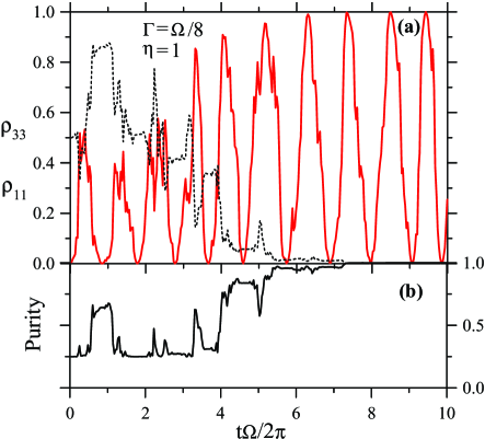
Figure 2: (Color online) Weak coupling regime, $\Gamma\ll\Omega$, at zero detuning. (a) A realization of $\rho_{33}(t)$ evolution (mixed initial state) showing collapse to the spin-singlet subspace $\{|1\rangle,|2\rangle\}$ (dashed line); weakly perturbed coherent oscillations of $\rho_{11}(t)$ (thick line) into the subspace. (b) Qutrit purification due to measurement with an ideal detector, $\eta=1$.

An example of the three-state system evolution is shown on Fig.2a. In this particular realization of the measurement process, while starting from a mixed initial state ($\rho_{11}(0)=0$, $\rho_{22}(0)=\rho_{33}(0)=1/2$, $\rho_{ij}(0)=0,i\neq j$) $\rho_{33}(t)\to 0$ (dashed line on Fig.2a), i.e., the system is continuously collapsed to the spin-singlet subspace, $\{|1\rangle\equiv|S(0,2)\rangle,|2\rangle\equiv|S(1,1)\rangle\}$ after a transition time of the order of $1/\Gamma$. On the same time scale, weakly perturbed quantum oscillations are established in this subspace [solid line on Fig.2a) for $\rho_{11}(t)$].

The oscillation scenario in case of collapse to the singlet subspace is easily understood. Once $\rho_{33}(t)$ gets to zero, Eqs.(15),(17) just become of the same form as that describing quantum oscillations for a single qubit.Kor-osc For zero detunning, $\mbox{Re}\rho_{12}$ decouples ($\mbox{Re}\rho_{12}(t)\rightarrow 0$), while $\rho_{11}(t)-\rho_{22}(t)=\cos[\Omega t+\varphi(t)]$ and $2\mbox{Im}\rho_{12}(t)=\sin[\Omega t+\varphi(t)]$ oscillate with a unity amplitude (for $\eta=1$), with phase $\varphi(t)$ that slowly diffuses in time.Kor-osc Correspondingly, the oscillating scenario can be distinguished by the average current $\langle I(t)\rangle_{t}=(I_{(0,2)}+I_{(1,1)})/2$ or by the current spectral density $S_{I}(\omega)=2\int_{-\infty}^{\infty}K_{I}(\tau)\exp(i\omega\tau)d\tau$ (with $K_{I}(\tau)=\langle I(t)I(t+\tau)\rangle_{t}-\langle I(t)\rangle_{t}^{2}$ being the current correlation function). Since the evolution of $\rho_{33}(t)$ is transitional in character (see Fig.2), it will not affect the long-time average $K_{I}(\tau)$. Then using, e.g., the methods of Ref.Ruskov-Zeno, , it can be shown that the detector power spectrum will have the same form as in the one-qubit caseKor-osc for any DQD parameters, $\delta$, $\Omega$. In particular, in the weak coupling regime (for $\delta=0$) the spectrum $S_{I}(\omega)$ exhibits a Lorenzian peak at the Rabi frequency $\Omega$ with a signal-to-noise ratio of $4\eta$, and a width $\Gamma=(I_{(0,2)}-I_{(1,1)})^{2}/4S_{0}\eta$.

On (Fig.2b) the qutrit purity is plotted. [We have defined it as $\mbox{Pur}(t)=(3\mbox{Tr}[\hat{\rho}(t)^{2}]-1)/2$, so that $\mbox{Pur}=1$ for a pure state and $\mbox{Pur}=0$ for a totally mixed state.] It is seen that the qutrit is eventually reaching a pure state [even though with a random phase, $\varphi(t)$] for a time of the order of $1/\Gamma$. The purification of the qutrit state is yet another demonstration of non-trivial interplay of dynamics. Indeed, Hamiltonian evolution alone conserves purity, while a measurement alone leaves states $|2\rangle$ and $|3\rangle$ unresolved. The purification of the state is due to an effective resolution of the states $|2\rangle$ and $|3\rangle$ and the fact that no information is lost with an ideal measurement.

For a measurement with a non-ideal detector, $\eta<1$, simulations show (if collapse happened to the spin-singlet subspace) that the amplitude of quantum oscillations is less than $1$ and fluctuates in time. Correspondingly, the average purity $\langle\mbox{Pur}(t)\rangle_{t}$ saturates at some lower value. Using Eqs.(15)-(19) we have derived in the weak coupling regime (compare with Ref.QinRusKor ) $\langle Pur(t)\rangle_{t}\simeq 1+(3/4)[1/2\eta-\sqrt{(1+1/2\eta)^{2}-2}]$ so that the qutrit state remains mixed; for small $\eta$ the qutrit purity approaches $1/4+3/2\eta$.

If collapse happens to $\rho_{33}(t)\to 1$, the state will purify even for measurement with a non-ideal detector. In this scenario the average current is $I_{(1,1)}$ and the power spectrum is flat, $S_{I}(\omega)=S_{0}$ [the detector signal is just $I(t)=I_{(1,1)}+\xi(t)$].

III.3 Large coupling. Zeno stabilization and emergence of negative-result evolution

We now turn to the case of relatively large system detector coupling, $\Gamma\gg\Omega$; the DQD detuning energy, $\delta$, can be either small or large. Numerical simulations confirm that collapse scenarios remain the same in the large coupling regime consistent with our argumentation in Sec. III A. However, in the strong coupling case the evolution qualitatively changes; the typical collapse time to either of the subspaces, {$|1\rangle,|2\rangle$} or $|3\rangle$, becomes much longer than $1/\Gamma$. Also, instead of quantum oscillations within the spin-singlet subspace $\{|1\rangle\equiv|S(0,2)\rangle$, $|2\rangle\equiv|S(1,1)\rangle\}$, associated with $\Omega$, we have relatively long stabilization of the system state (Fig. 3) in one of the two states since the measurement is trying to localize and “freeze” the system in a definite charge state. This is a manifestation of the quantum Zeno effect:Khalfin ; MisraSudarshan in the case of continuous measurement the detector is always coupled to the system, so the approach to quantum Zeno regime corresponds to the limit of stronger and stronger coupling. For a finite coupling the long stabilization periods will be interrupted by rare switching events between the subspaces (the switching transition time is of the order of $1/\Gamma$; see below).

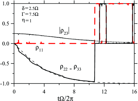
Figure 3: (Color online) Strong coupling regime, $\Gamma\gg\Omega$. Zeno stabilization in the qubit subspace, $\rho_{11}=0$, for a long time until it switches to $\rho_{11}=1$ (thick dashed line). The noisy qubit evolution of a mixed initial state shown for $\rho_{22}-\rho_{33}$ and $|\rho_{23}|$ vs. postulated negative-result evolution given by Eqs.(27)-(29) (long dashed and short dashed lines).

Anticipating the scenario of a negative-result evolution in the qubit subspace outlined in the beginning of Sec. III, we turn to the calculation of the switching rate between the two singlet states, which will set the time scale of non-unitary dynamics. From an ensemble averaged point of view the qubit “decay” from $|S(1,1)\rangle$ to $|S(0,2)\rangle$ (triplet state $|T_{0}(1,1)\rangle$ is spin blocked) is described as a smooth decrease of $\langle\rho_{11}(t)\rangle$ and therefore the switching rate would be most easily obtained if we consider the master equation (13) that follows from averaging of measurement evolution.

Due to current level degeneracy, $I_{2}=I_{3}=I_{(1,1)}$, the dephasing rate $\Gamma_{23}$, Eq.(14), vanishes just because the detector cannot distinguish between the corresponding states (no information can be obtained and therefore no information can be lost). Introducing $\Gamma_{12}=\Gamma_{13}=\Gamma\equiv(\Delta I)^{2}/4S_{0}\eta$ the master equation reads

$$\langle\dot{\rho}_{kl}\rangle=-\frac{i}{\hbar}[{\cal H}_{DQD},\langle\rho\rangle]_{kl}$$ (24)

$$\qquad{}-\Gamma\ \left(\begin{array}[]{ccc}0&\langle\rho_{12}\rangle&\langle\rho_{13}\rangle\\ \langle\rho_{21}\rangle&0&0\\ \langle\rho_{31}\rangle&0&0\\ \end{array}\right)_{kl}$$

In order to calculate the switching rate from the state $|1\rangle=|S(0,2)\rangle$ we start with the initial condition $\rho_{11}=1$. Using Eq.(LABEL:Master) one derives the small time evolution:

$$\langle\rho_{11}(t)\rangle=1-\frac{\Omega^{2}t^{2}}{4}+\cdots.$$ (25)

Notice, that there is no linear term in the expansion, Eq.(25), which tells us that the decay is not exponential at a small time scale. This fact makes quantum Zeno effect physics possible. The $t^{2}$-coefficient turns out to be $-(\Omega)^{2}/4=-\mbox{Tr}[\hat{\rho}^{2}{\cal H}^{2}_{DQD}]+\mbox{Tr}[\hat{\rho}{\cal H}_{DQD}\hat{\rho}{\cal H}_{DQD}]$, i.e. it is determined by coherent (Hamiltonian) evolution alone, consistent with the discussion in Refs. Khalfin, ; MisraSudarshan, ; Peres, .

It is instructive to find an approximate solution for $\langle\rho_{11}(t)\rangle$ considering in (LABEL:Master) terms proportional to $\Omega$ as a small perturbation ($\Omega\ll\Gamma$, for strong coupling). To first order in the perturbation $\Omega$ we obtain for $\mbox{Im}\langle\rho_{12}(t)\rangle$:

$$\mbox{Im}\langle\rho_{12}(t)\rangle=e^{-\Gamma t}\,\left[\mbox{Re}\rho_{12}(0)\,\sin{\delta t}+\mbox{Im}\rho_{12}(0)\,\cos{\delta t}\right]$$ (26)

$$\ {}+\frac{\Omega}{\Gamma^{2}+\delta^{2}}\,\left\{\frac{\Gamma}{2}+e^{-\Gamma t}\,\left[\delta\,\sin{\delta t}-\Gamma\cos{\delta t}\right]\right\}.$$

Using the relation, $\langle\rho_{11}(t)\rangle=\rho_{11}(0)-\Omega\int_{0}^{t}\mbox{Im}\langle\rho_{12}(t^{\prime})\rangle dt^{\prime}$, we can obtain an approximate solution for $\langle\rho_{11}(t)\rangle$ and its small $t$ expansion coincides with first few terms of the expansion, Eq.(25). However on a time scale $t^{*}\gtrsim 1/\Gamma$, as seen in Eq.(26), the exponential terms drop out and one reaches an expansion that has a linear term: $\langle\rho_{11}(t^{*})\rangle\simeq 1-\frac{\Omega^{2}\Gamma}{2(\Gamma^{2}+\delta^{2})}\,t^{*}$. Similarly, one can show that if one starts from an initial state in the {$|2\rangle$, $|3\rangle$}-subspace then on a coarse grained time scale $\langle\rho_{22}(t^{*})\rangle\simeq\rho_{22}(0)\,\left[1-\frac{\Omega^{2}\Gamma}{2(\Gamma^{2}+\delta^{2})}\,t^{*}\right]$; $\langle\rho_{33}(t)\rangle$ is just conserved. By solving numerically the master equation (LABEL:Master) for $\langle\rho_{11}\rangle$, $\langle\rho_{22}\rangle$, $\mbox{Re}\langle\rho_{12}\rangle$, $\mbox{Im}\langle\rho_{12}\rangle$ one confirms that the decay of the subspaces is indeed exponential for large times and the switching rate between the subspaces is

$$\Gamma_{sw}=\frac{\Omega^{2}\Gamma}{2(\Gamma^{2}+\delta^{2})}.$$ (27)

Note that the strong coupling limit when $\Gamma\gg\Omega$ ($\delta$ is arbitrary) implies that $\Gamma_{sw}\ll\Gamma$, i.e. the subspace life time is much longer than both $1/\Gamma$ and $1/\Omega$ implying quantum Zeno stabilization.EnsAverageView The exponential decay at times $t^{*}\gtrsim 1/\Gamma$ is a sign of the irreversibility of the measurementPeres-book that appears as a switching event.

Having calculated the switching rate between the spin-charge states we can write (postulate) an ansatz for the time evolution of $\rho(t)$ according to a given result. Starting from the qubit subspace, for times $t^{*}\gtrsim 1/\Gamma$ one will be able to discriminate between the two current values ($I_{(1,1)}$ or $I_{(0,2)}$) and thus to distinguish whether the system has decayed (switched) to the third state or not. The conditional probability for the state $|2\rangle=|S(1,1)\rangle$ not to decay by time $t$ is given by $P_{2}(t)=\exp{(-\Gamma_{sw}t)}$, while analogous probability for $|3\rangle=|T_{0}(1,1)\rangle$ is $P_{3}(t)=1$ (due to spin-blockade). Using the quantum Bayes rule, similar to the two-level atom, Eqs.(1),(2) [see also Eq.(10)], one can write the effective negative-result evolution of the spin qubit subsystem given that it did not decay by time $t$:

$$\rho_{22}(t)=\frac{\rho_{22}(0)\,P_{2}(t)}{P_{tot}(t)},\ \rho_{33}(t)=\frac{\rho_{33}(0)}{P_{tot}(t)}\ \$$ (28)

$$\rho_{23}(t)=\rho_{23}(0)\,\sqrt{\frac{\rho_{22}(t)\,\rho_{33}(t)}{\rho_{22}(0)\,\rho_{33}(0)}}\ e^{-i\phi(t,\delta,\Omega,\Gamma)},\qquad$$ (29)

where the total probability not to decay is given by $P_{tot}(t)=\rho_{22}(0)\,P_{2}(t)+\rho_{33}(0)\,P_{3}(t)$, and $\phi(t,\delta,\Omega,\Gamma)$ is an accumulated phase (see below).

Consistency of the informational (Bayesian) approach requires that the negative-result ansatz for the $\rho(t)$-evolution be reproduced by the underlying evolution, Eq.(11), according to the noisy record $I(t)$. In Fig.3 we show the negative-result evolution for $\rho_{22}(t)-\rho_{33}(t)$ and $|\rho_{23}(t)|$ defined by Eqs.(27),(28),(29), versus the density matrix evolution generated through simulation of the noisy measurement process via Eqs.(11),(12). The (noisy) evolution in the qubit subspace is quite regular, and the state eventually approaches $|3\rangle\equiv|T_{0}(1,1)\rangle$ (if the system did not switch). One can see that the two evolutions well agree in the strong coupling regime; the agreement is already established at $\Gamma\gtrsim 5\Omega$. The agreement reveals a non-trivial property of the Bayesian stochastic evolution Eq. (11). It means that the postulated negative-result evolution given by Eqs.(28), (29), can be actually derived from Eq. (11) in the Zeno regime, as an interplay of measurement evolution and Hamiltonian evolution at an underlying microscopic level.

The time scale of the negative-result evolution is set by the switching rate $\Gamma_{sw}$, Eq.(27), in which the detector rate $\Gamma=(\Delta I)^{2}/4S_{0}\eta\equiv(\Delta I)^{2}/4S_{0}+\gamma_{12}$ is the total rate, including the measurement rate and the additional rate due to detector non-ideality. Via numerical simulations we have confirmed the dependence of $\Gamma_{sw}$ on $\eta$. We note that while the rate $\gamma_{12}$ would lead to dephasing in the spin-singlet subspace {$|1\rangle,|2\rangle$} [see Eq.(17)], it affects the spin qubit coherentlynon-ideality-neg in the sense that Eq.(29) preserves the coherence ratio $|\rho_{23}|/\sqrt{\rho_{22}\,\rho_{33}}$. The reason is the indistinguishability of the states $|S(1,1)\rangle$ and $|T_{0}(1,1)\rangle$ by the measurement. Particularly, a pure state remains pure, which we have confirmed numerically. (A similar conclusion was drawn in Ref.Pryadko, from a completely different viewpoint.) The mixed state will generally purify (see the discussion in Ref.Ruskov-neg, ). The final qubit (and qutrit) purification happens on the same time scale $\Gamma_{sw}^{-1}\gg\Gamma^{-1}$ as the collapse to the spin-singlet or spin-triplet subspaces.

The update for the non-diagonal element $\rho_{23}$ in (29) reflects not only the conservation of coherence, but includes an accumulated phase $\phi(t,\delta,\Omega,\Gamma)$, which remains undefined by the negative-result ansatz. Stochastic numerical simulations by Eqs.(11),(12) show that the phase is linear in time even for small detuning, $|\delta|\lesssim\Omega$: $\phi(t)=\varepsilon^{\mbox{\small eff}}_{23}(\delta,\Omega,\Gamma)\,t$ and vanishes for $\delta=0$ (while noisy, it stabilizes just for times $\gtrsim 1/\Gamma$). The coefficient $\varepsilon^{\mbox{\small eff}}_{23}$ can be interpreted as an energy splitting between the spin qubit states $|2\rangle$ and $|3\rangle$ induced by the negative-result measurement in the presence of the localized singlet state, $|1\rangle$. For small detuning, $\delta\sim\Omega$, the energy splitting is small, $|\varepsilon^{\mbox{\small eff}}_{23}|\ll|\varepsilon^{pert}_{23}|\simeq\frac{\Omega^{2}}{4|\delta|}$; it has the same sign as the exchange splitting, $\varepsilon^{pert}_{23}$, that would be induced perturbatively.

The effective energy splitting can be derived if one compares ensemble averaging of the negative-result evolution given by Eqs.(28),(29) with the ensemble averaged evolution of the “original” stochastic equations (11). Since the negative-result evolution is the Bayesian evolution at a coarse grained time scale $t^{*}\gtrsim 1/\Gamma$, its ensemble averaging must coincide with the evolution given by the master equation (LABEL:Master) considered at times $\gtrsim 1/\Gamma$. Averaging of the negative-result evolution is straightforward using the probability not to decay, $P_{tot}(t)$. Starting from the qubit subspace it gives, e.g., for the non-diagonal matrix element:

$$\langle\rho_{23}(t)\rangle=\rho_{23}(0)\,e^{-\Gamma_{sw}\,t/2}\,e^{-i\,\varepsilon^{\mbox{\footnotesize eff}}_{23}\,t}.$$ (30)

On the other hand Eq.(LABEL:Master) gives for the ensemble averaged evolution of $\langle\rho_{23}(t)\rangle$, $\langle\rho_{13}(t)\rangle$:

$$\langle{\dot{\rho}}_{23}(t)\rangle=-i\,\frac{\Omega}{2}\langle\rho_{13}(t)\rangle$$ (31)

$$\langle{\dot{\rho}}_{13}(t)\rangle=i\,\delta\,\langle\rho_{13}(t)\rangle-i\,\frac{\Omega}{2}\,\langle\rho_{23}(t)\rangle-\Gamma\,\langle\rho_{13}(t)\rangle.\qquad\$$ (32)

It can be solved exactly, and for the initial values $\rho_{13}(0)=0$, $\rho_{23}(0)$, we obtain:

$$\langle\rho_{23}(t)\rangle=\rho_{23}(0)\,e^{-\tilde{\Gamma}t/2}\,\left(\cosh{\tilde{\Omega}t}+\frac{2\tilde{\Gamma}}{\tilde{\Omega}}\,\sinh{\tilde{\Omega}t}\right)$$ (33)

where $\tilde{\Gamma}\equiv\Gamma-i\,\delta$, $\tilde{\Omega}\equiv\sqrt{\tilde{\Gamma}^{2}-\Omega^{2}}/2$. Taking the strong coupling limit $\Gamma\gg\Omega$ ($\delta$ is arbitrary), at times $t^{*}\gtrsim 1/\Gamma$ when some contributions to Eq.(33) are exponentially suppressed [similar to Eq.(26)], we reproduce the evolution for $\langle\rho_{23}(t)\rangle$, Eq.(30), with an energy splitting:

$$\varepsilon^{\mbox{\small eff}}_{23}(\delta,\Omega,\Gamma)=\frac{\Omega^{2}\delta}{4(\Gamma^{2}+\delta^{2})}=\Gamma_{sw}\frac{\delta}{2\Gamma};$$ (34)

it approaches $\varepsilon^{pert}_{23}\simeq\frac{\Omega^{2}}{4\delta}$ for large $\delta$. Eq.(34) is confirmed with a very good accuracy by the results obtained through direct simulation of the stochastic Bayesian evolution equations (11). Eqs.(28),(29),(34) suggest that the spin-charge states under continuous strong measurement can be re-interpreted as the “new” energy states, if the quantum evolution is monitored at times $t^{*}\gtrsim 1/\Gamma$.

III.4 Zeno stabilization at small coupling and large detuning

Interestingly, Zeno stabilization can take place even at small coupling, if the detuning is sufficiently large, $\Gamma\ll\Omega\ll\delta$. Qualitatively, this can be understood by kinematical reasons as illustrated on the spin-singlet Bloch sphere, Fig.4. In the stochastic Bayesian equations (11), for large detuning $\delta\gg\Omega$, the Hamiltonian evolution is a fast rotation with $\Omega_{sys}=\sqrt{\delta^{2}+\Omega^{2}}$ around an axis close to the $z$-axis. On the other hand, the measurement alone tries to localize the state to either of the poles (the singlet states) acting along the meridians. The angular velocity along the meridians is $\Omega\ll\Omega_{sys}$; also the oscillation amplitude is $\sim\frac{\Omega}{\delta}\ll 1$, so that the Hamiltonian evolution is effectively suppressed due to averaging. Thus, even though the coupling is small, $\Gamma\ll\Omega$, it might be large with respect to an effective evolution rate along the meridians which quantifies a quantum Zeno effect. Numerical simulation of noisy measurement evolution shows that the DQD two-electron system either collapses to the spin-singlet subspace (similar to that shown in Fig.3), or ends up at the triplet state. In the first scenario, the system is stabilized for a relatively long time $\Gamma_{sw}^{-1}\gg\Gamma^{-1}$ in one of the singlet states while performing rare switchings between them.

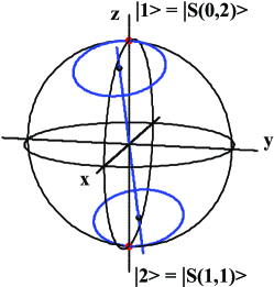
Figure 4: (Color online) Bloch sphere in the spin-singlet subspace illustrates the Zeno stabilization in case of weak coupling and large detuning. The projection of the Hamilton evolution (rotation around an axis close to $z$-axis) along the meridians (measurement evolution) is effectively small.

The switching rate $\Gamma_{sw}$ is given by the same formula, Eq.(27), since the $\Omega$-terms in the master equation are still small perturbations with respect to the remaining terms as in Eq.(26). Solution of the master equation (LABEL:Master) confirms that at a time scale $t^{*}\geq 1/\Gamma$ the decay from the subspaces is exponential as was in the case of a strong coupling, with the same switching rate. Correspondingly, numerical simulation of noisy measurement evolution of the DQD two-electron system, as shown on Fig.5a,b, is in a good agreement with the negative-result evolution described by Eqs.(28),(29). Generally, the agreement is established already at $\delta\gtrsim 3\Omega$. Here, the initial qubit state was chosen to be a pure state and it remains pure as well as the purity of the total qutrit state (not shown). The negative-result evolution in the spin qubit subspace takes place as long as the system did not switch to the third state. In Fig.5 a realization of the measurement process is shown when the system did not switch at all. Indeed, in a situation when only a $\sigma_{z}$-evolution is present in addition to the negative-result evolution, Eqs.(28),(29), the probability not to decay is given by $P_{tot}(t)=\rho_{33}(0)+\rho_{22}(0)e^{-\Gamma_{sw}t}$. So, it approaches $\rho_{33}(0)$, remaining finite for large times.

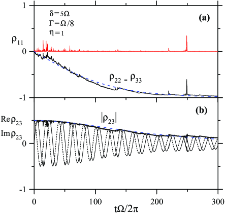
Figure 5: (Color online) Evolution in the regime of small coupling and large detuning. (a) A realization when the qubit did not switch: $\rho_{11}(t)$ remains zero always. Evolution of $\rho_{22}-\rho_{33}$ shows collapse to the state $|3\rangle\equiv|T_{0}(1,1)\rangle$. (b) Oscillation of coherences, $\mbox{Re}\rho_{23}$ and $\mbox{Im}\rho_{23}$ (thin dashed and solid lines), and their envelop $|\rho_{23}|$ (thick solid line) vs. negative-result evolution of $|\rho_{23}|$ (dashed line) according to Eqs.(27)-(29).

The induced energy splitting leads to a $\sigma_{z}$ evolution for $\mbox{Re}\rho_{23}$, $\mbox{Im}\rho_{23}$, whose amplitude envelope is provided by the negative-result evolution, Fig.5b. For large detuning and small coupling the energy splitting is mainly due to perturbative influence of the third state: $\varepsilon^{\mbox{\small eff}}_{23}\simeq\varepsilon^{pert}_{23}=\Omega^{2}/4\delta$ as it follows from Eq.(34).

IV Available experimental parameters

1. Coupling strength and switching rate. The possibility to detect single electronic charges in quantum dots (QD) via quantum point contact or single electron transistor was recently demonstrated in experiments of different groups. Marcus-Sci ; Kouw-prl94 ; Rimberg-nat The detector coupling, $\Gamma=(\Delta I)^{2}/4S_{0}\eta$, essentially determines the measurement time $\tau_{meas}\sim 1/\Gamma$ to reach a signal-to-noise ratio of order one, where $\Delta I$ is the current difference signal in the detector due to the presence (or absence) of an extra electron charge $e$ in the QD. For the charge sensitivity of an rf-SET $\delta q=2.4\times 10^{-5}e/\sqrt{Hz}$, provided in Ref.Rimberg-nat, , one estimates $\Gamma^{SET}_{exp}\approx 10^{7}\,s^{-1}$. Recent experiment of Rimberg groupRimberg-new2 demonstrated a charge sensitivity of an rf-SET of $\delta q=2.4\times 10^{-6}e/\sqrt{Hz}$. Due to quadratic dependence on sensitivity, $\Gamma\propto(\delta q)^{-2}$, this amounts to a two orders of magnitude improvement,improvement $\Gamma^{SET}_{exp}\simeq 10^{9}\ s^{-1}$. For an rf-QPC,rf-QPC we estimated $\Gamma^{QPC}_{exp}\simeq 10^{6}\ s^{-1}$. The high detector ideality of a QPC also may be lost in the rf-regime.Gambetta

The above estimates show that, in principle, both a weak coupling as well as a strong coupling regime of a negative-result evolution are experimentally reachable. For a typical tunneling,Taylor $t_{c}\approx 10\ \mu eV$ the characteristic frequency $\Omega=2\,t_{c}/\hbar\approx 3\times 10^{10}\ s^{-1}$ is large. Given the range of DQD detuning, $|\delta|\approx 0-300\ \mu eV$, one can reach a quantum Zeno stabilization if a relatively large detuning is taken. Smaller values of tunneling, $t_{c}\approx 1\ \mu eV$ or even $t_{c}\approx 0.1\ \mu eV$, are also reachableKouwenhoven-Sci so that a strong coupling regime may be realized. Typical values of switching rate $\Gamma_{sw}$ for the presented parameters are in the range $2\times 10^{5}-5\times 10^{7}s^{-1}$.

2. Decoherence due to charge fluctuations. The decoherence in the DQD two-electron system has various sources. The coupling to uncontrollable detector degrees of freedom leads to detector non-ideality, $\eta$, partially discussed in Section II. Another mechanism of decoherence is due to systems’s coupling to background charge fluctuationsCoishLoss ; HuDasSarma ; Taylor ; RomitoGefen that will lead to a non-zero dephasing $\gamma_{23}$ in the spin-qubit subspace. It was arguedCoishLoss ; HuDasSarma ; Taylor that such dephasing will be well suppressed in the far-detuned regime $\delta\gg t_{c}$, where it may be $\gamma_{23}\approx 10^{3}-10^{5}\ s^{-1}$. However, close to the charge degeneracy, $\delta\lesssim t_{c}$, the dephasing may strongly increaseHuDasSarma ; RomitoGefen to $\gamma_{23}\approx 10^{6}-10^{7}\ s^{-1}$ due to higher sensitivity to fluctuations of the DQD parameters. In the latter case it will be difficult to see the effect of Zeno stabilization since $\gamma_{23}$ becomes comparable to the switching rate $\Gamma_{sw}$.

3. Decoherence due to phonons. Yet another decoherence mechanism (also related to charge degrees of freedom) is due to coupling to a phonon environment.LeggettRevModPhys ; Brandes Physically, the relevant process is the double-dot inelastic tunnelingMarcus-Sci ; Kouwenhoven-Sci from state $|2\rangle=|S(1,1)\rangle$ to state $|1\rangle=|S(0,2)\rangle$ quantified by the inelastic rate $\Gamma_{in}(\delta)$. Relaxation process associated with the inelastic tunneling may lead to a contribution to the switching rate $\Gamma_{sw}$, assuming a weak environment, $\Gamma_{in}\ll\Omega,\Gamma$. Associated contribution to the dephasing $\gamma_{12}$ (also of the order of $\Gamma_{in}$) is expected not to destroy the negative-result evolution in this case.

Estimations of the inelastic rateTaylor give the range of $0.01-100neV$ (corresponding to approximately $10^{4}-10^{8}\ s^{-1}$) depending on the energy splitting $\Delta E$ between the relevant states. Due to generic cubic dependence on the splitting, $\Gamma_{in}\propto(\Delta E)^{3}$, one can hope to find a range of not too large detuning $\delta$ so that $\Gamma_{in}$ is in the range of $10^{4}-10^{5}\ s^{-1}$. Thus, eventually one may expect to manage the inequality $\Gamma_{in}\ll\Gamma_{sw}$, so that the Zeno stabilization will effectively “fight” against decoherence. We note that various models of boson environment may affect the predicted negative-result evolution in different ways that deserve a separate investigation.

4. Implications of the QD nuclei. The contact hyperfine interaction of the electron spins with the surrounding nuclei spins in the DQD leads to entanglement with the uncontrolable spin-bath degrees of freedom;Dobrovitski ; Dobrovitski1 ; Zurek ; Glazman in quasi-classical language it can be described as an effect of “inhomogeneous broadening” quantified by the random nuclear Overhauser field. nuclear-quasistatic ; Taylor ; Dobr1 ; Dobrovitski-rev The dephasing caused by such effects in the spin qubit have been experimentally measuredMarcus-Sci ; HansonReview (dephasing time is of the order of $\sim 10^{-8}\ s$); such strong dephasing may conceal any interesting quantum evolution. For a non-interacting bath it was shown that this type of decoherence can be completely eliminated by using various spin-echo techniques.Witzel Realistically, for a weakly interacting bath, application of such techniques would reduce the decoherence by a few orders of magnitude.Witzel ; Zhang For a GaAs DQD spin qubit system a “true” decoherence time of the order of $\sim 10^{-6}\ s$ was measured experimentally using simple spin-echo.Marcus-Sci ; HansonReview

This suggests that spin-echo techniques could be of use also to reveal the negative-result evolution we are discussing in this paper. We leave for a future project the investigation of various possibilities for application of spin-echo techniques in conjunction with a negative-result measurement evolution in the context of manipulation and/or preparation of the state of a DQD spin qubit.

V Conclusion

We have shown that a negative-result evolution of a spin qubit can effectively emerge out of noisy measurement of a DQD spin system by a linear detector such as a quantum point contact. The evolution emerges as an interplay of measurement (non-unitary) dynamics and Hamiltonian dynamics of the three-level system, when quantum Zeno stabilization of the spin qubit subspace takes place.

Besides implications to the theory of quantum measurements, our results may be of practical use for manipulation of a DQD spin qubit (for papers discussing quantum measurements as an important resource see, e.g., Refs.RusKor-ent, ; KorJordan-undo, ; Ruskov-neg, ; prl-quadr, ; Beenakker, ; EngelLoss, ; Jordan-neg, ; Nori, ). Recent experiments on a single phase qubit provide an interesting manipulation of its state via negative-result measurement.Katz-Sci ; Katz-Nature These advances support the hope that experimental implementation of negative-result evolution is also possible in a DQD spin qubit system.

References

- (1) R. Hanson, L. P. Kouwenhoven, J. R. Petta, S. Tarucha, and L.M.K. Vandersypen, Rev. Mod. Phys. 79, 1217 (2007)
- (2) M. Pioro-Ladriere, T. Obata, Y. Tokura, Y.-S. Shin, T. Kubo, K. Yoshida, T. Taniyama, and S. Tarucha, Nature Physics 4, 776 (2008).
- (3) E. A. Laird, C. Barthel, E. I. Rashba, C. M. Marcus, M. P. Hanson, and A. C. Gossard, Phys. Rev. Lett. 99, 246601 (2007)
- (4) J. Berezovsky, M. H. Mikkelsen, N. G. Stoltz, L. A. Coldren, and D. D. Awschalom, Science 320, 349 (2008).
- (5) F. H. L. Koppens, K. C. Nowack, and L. M. K. Vandersypen Phys. Rev. Lett. 100, 236802 (2008).
- (6) J. Dalibard, Y. Castin, and K. Mølmer, Phys. Rev. Lett. 68, 580 (1992).
- (7) H. J. Carmichael, An Open System Approach to Quantum Optics (Springer, Berlin, 1993).
- (8) H. M. Wiseman and G. J. Milburn, Phys. Rev. Lett. 70, 548 (1993); Phys. Rev. A 49, 1350 (1994).
- (9) A. N. Korotkov, Phys. Rev. B 63, 115403 (2001); Phys. Rev. B 60, 5737 (1999).
- (10) P. S. Epstein, Am. J. Phys. 13, 127 (1945); M. Renninger, Zeitschr. für Physik 158, 417 (1960); R. H. Dicke, Am. J. Phys. 49, 925 (1981); D. T. Pegg and P. L. Knight, Phys. Rev. A 37, 4303 (1988).
- (11) N. Katz, M. Ansmann, R. C. Bialczak, E. Lucero, R. McDermott, M. Neeley, M. Steffen, E. M. Weig, A. N. Cleland, J. M. Martinis, and A. N. Korotkov, Science, 312 1498 (2006).
- (12) L. P. Pryadko and A. N. Korotkov, Phys. Rev. B 76, 100503(R) (2007).
- (13) D. Loss and D. P. DiVincenzo, Phys. Rev. A 57, 120 (1998).
- (14) J. Elzerman, R. Hanson, L. H. Willems van Beveren, B. Witkamp, L. M. K. Vandersypen, and L. P. Kouwenhoven, Nature 430, 431 (2004).
- (15) J. R. Petta, A. C. Johnson, J. M. Taylor, E. A. Laird, A. Yacoby, M. D. Lukin, C. M. Marcus, M. P. Hanson, and A. C. Gossard, Science 309, 2180 (2005).
- (16) R. Hanson, L. H. Willems van Beveren, I. T. Vink, J. M. Elzerman, W. J. M. Naber, F. H. L. Koppens, L. P. Kouwenhoven, and L. M. K. Vandersypen, Phys. Rev. Lett. 94, 196802 (2005).
- (17) W. Lu, Z. Ji, L. Pfeifer, K. W. West, and A. J. Rimberg, Nature 423, 422 (2003).
- (18) A. N. Korotkov and D. V. Averin, Phys. Rev. B 64, 165310 (2001); A. N. Korotkov, Phys. Rev. B 63, 085312 (2001).
- (19) R. Ruskov, A. Mizel, and A. N. Korotkov, Phys. Rev. B 75, 220501(R)(2007).
- (20) R. Ruskov and A. N. Korotkov, Phys. Rev. B 67, 241305 (2003).
- (21) R. Ruskov, A. N. Korotkov, and A. Mizel, Phys. Rev. B 73, 085317 (2006).
- (22) L.S. Khalfin, JETP Lett. 8, 63 (1968).
- (23) B. Misra and E. C. G. Sudarshan, J. Math. Phys. 18, 756 (1977); C.B Chiu, E. C. G. Sudarshan, and B. Misra, Phys. Rev. D 16, 520 (1977).
- (24) A. Peres, Am. J. Phys. 48, 931 (1980).
- (25) A. N. Korotkov and A.N. Jordan, Phys. Rev. Lett. 97, 166805 (2006).
- (26) F. H. L. Koppens, J. A. Folk, J. M. Elzerman, R. Hanson, L. H. Willems van Beveren, I. T. Vink, H. P. Tanitz, W. Wegscheider, L. P. Kouwenhoven, and L. M. K. Vandersypen, Science 309, 1346 (2005).
- (27) J. M. Taylor, J. R. Petta, A. C. Johnson, A. Yacoby, C. M. Marcus, and M. D. Lukin, Phys. Rev. B 76, 035315 (2007).
- (28) O. N. Jouravlev and Yu. Nazarov, Phys. Rev. Lett. 96, 176804 (2006).
- (29) C. M. Caves and G. J. Milburn, Optics Communications 179, 439 (2000).
- (30) S. A. Gurvitz, Phys. Rev. B 56, 15215 (1997).
- (31) E. B. Davies, Quantum Theory of Open Systems, (Academic, London, 1976).
- (32) A. S. Holevo, Statistical Structure of Quantum Theory, (Springer, Berlin, 2001).
- (33) A. Shnirman and G. Schön, Phys. Rev. B 57, 15400 (1998).
- (34) A. N. Korotkov, Phys. Rev. A 65, 052304 (2002).
- (35) D. V. Averin and E. V. Sukhorukov, Phys. Rev. Lett. 95, 126803 (2005).
- (36) A. N. Jordan and A. N. Korotkov, Phys. Rev. B 74, 085307 (2006).
- (37) M. A. Nielsen and I. L. Chuang, Quantum Computation and Quantum Information, (Cambridge University Press, Cambridge, 2000).
- (38) Independent tunneling events amount to the requirement of high detector voltage as mentioned in Sec. II.1. Number of classical tunneling attempts per second can be evaluated as , consistent with the Landauer formula for average currents, given just after Eq.(6).
- (39) B.Øksendal, Stochastic differential equations (Springer, Berlin, 1998).
- (40) D. V. Averin, Fortschr. Phys. 48, 1055 (2000); H. S. Goan and G. J. Milburn, Phys. Rev. B 64, 235307 (2001); A. A. Clerk, S. M. Girvin, and A. D. Stone, Phys. Rev. B 67, 165324 (2003); A. N. Jordan and M. Buttiker, Phys. Rev. Lett. 95, 220401 (2005).
- (41) R. Ruskov, A. N. Korotkov, and A. Mizel, Phys. Rev. Lett. 96, 200404 (2006).
- (42) E. Buks, R. Schuster, M. Heiblum, D. Mahalu, and V. Umansky, Nature 391, 871 (1998).
- (43) A. B. Zorin, Phys. Rev. Lett. 76, 4408 (1996); D. V. Averin, cond-mat/0010052 (unpublished); A. A. Clerk, S. M. Girvin, A. K. Nguyen, and A. D. Stone, Phys. Rev. Lett. 89, 176804 (2002).
- (44) A. O. Caldeira and A. J. Leggett, Ann. Phys. (N.Y.) 149, 374 (1983); W. H. Zurek, Physics Today 44, 36 (1991).
- (45) Qin Zhang, R. Ruskov, and A. N. Korotkov, Phys. Rev. B 72, 245322 (2005).
- (46) From an ensemble averaged point of view, when the result of the QPC is ignored, any qutrit state will be “frozen” for times .
- (47) A. Peres, Quantum Theory: Concepts and Methods (Kluwer Academic Publishers, The Netherlands, 1995).
- (48) Generally, we expect that possible presence of dephasing in Eq. (29), e.g. a factor , will be strongly suppressed in the Zeno regime: (compare with Ref.Kor-fidelity ).
- (49) A. N. Korotkov, Phys. Rev. B 78, 174512 (2008).
- (50) W. W. Xue, B. Davis, F. Pan, J. Stettenheim, T. J. Gilheart, A. J. Rimberg, and Z. Ji, Appl. Phys. Lett. 91, 093511 (2007).
- (51) There is a room for a factor of improvement of the charge sensitivity (depending on the SET operational temperatureDelsing ) until reaching the theoretical limit obtained in Ref.KorotkovPaalanen,
- (52) H. Brenning, S. Kafanov, T. Duty, S. Kubatkin, and P. Delsing, J. of Appl. Phys. 100, 114321 (2006).
- (53) A. N. Korotkov and M. A. Paalanen, Appl. Phys. Lett. 74, 4052 (1999).
- (54) D. J. Reilly, C. M. Marcus, M. P. Hanson, and A. C. Gossard, Appl. Phys. Lett. 91, 162101 (2007); M. Thalakulam, W. W. Xue, F. Pan, Z. Ji, J. Stettenheim, Loren Pfeiffer, K.W. West, and A. J. Rimberg, “Shot-Noise-Limited Operation of a Fast Quantum-Point-Contact Charge Sensor” cond-mat.mes-hall/0708.0861 (2007).
- (55) N. P. Oxtoby, J. Gambetta, and H.M. Wiseman, Phys. Rev. B 77, 125304 (2008).
- (56) W. A. Coish and D. Loss, Phys. Rev. B 72, 125337 (2005).
- (57) X. Hu and S. Das Sarma, Phys. Rev. Lett. 96, 100501 (2006).
- (58) A. Romito and Y. Gefen, Phys. Rev. B 76, 195318 (2007).
- (59) A. J. Leggett, S. Chakravarty, A. T. Dorsey, M. P. A. Fisher, A. Garg, and W. Zwerger, Rev. Mod. Phys. 59, 1 (1987).
- (60) T. Brandes and B. Kramer, Phys. Rev. Lett. 83, 3021 (1999); T. Brandes and T. Vorrath, Phys. Rev. B 66, 075341 (2002).
- (61) V. V. Dobrovitski et al., quant-ph/0112053; W. Zhang, V. V. Dobrovitski, K.A. Al-Hassanieh, E. Dagotto, and B.N. Harmon, Phys. Rev. B 74, 205313 (2006).
- (62) V. V. Dobrovitski, H. A. De Raedt, M. I. Katsnelson, B. N. Harmon, Phys. Rev. Lett. 90, 210401 (2003).
- (63) F. M. Cucchietti, J.P. Paz, and W. H. Zurek, Phys. Rev. A 72, 052113 (2005).
- (64) A. V. Khaetskii, D. Loss, and L. Glazman, Phys. Rev. Lett. 88, 186802 (2002).
- (65) I. A. Merkulov, A. L. Efros, and J. Rosen, Phys. Rev. B 65, 205309 (2002); S. I. Erlingsson and Yu. V. Nazarov, Phys. Rev. B 66, 155327 (2002).
- (66) V. V. Dobrovitski, A. E. Feiguin, D. D. Awschalom, and R. Hanson, Phys. Rev. B 77, 245212 (2008).
- (67) W. M. Witzel, R. de Sousa, and S. Das Sarma, Phys. Rev. B 72, 161306(R) (2005); W. M. Witzel, and S. Das Sarma, ibid 74, 035322 (2006); W. Yao, R.B. Liu and L.J. Sham, ibid 74, 195301 (2006); N. Shenvi, R. de Sousa, and K. B. Whaley, ibid 71, 224411 (2005).
- (68) W. Zhang, V. V. Dobrovitski, Lea F. Santos, Lorenza Viola, and B.N. Harmon, Phys. Rev. B 75, 201302 (2007).
- (69) W. Mao, D.V. Averin, R. Ruskov, and A. N. Korotkov, Phys. Rev. Lett. 93, 056803 (2004).
- (70) C. W. J. Beenakker, D.P. DiVincenzo, C. Emary, and M. Kindermann, Phys. Rev. Lett. 93, 020501 (2004).
- (71) H.-A. Engel and D. Loss, Science 309, 588 (2005).
- (72) A.N. Jordan, B. Trauzettel, G. Burkard, Phys. Rev. B 76, 155324 (2007).
- (73) W. X. Zhang, N. Konstantinidis, K. A. Al-Hassanieh, V. V. Dobrovitski, J. of Phys. - Cond. Mat. 19, 083202 (2007).
- (74) X.-B. Wang, J.Q. You, and F. Nori, Phys. Rev. A 77, 062339 (2008).
- (75) N. Katz, M. Neeley, M. Ansmann, R. C. Bialczak, M. Hofheinz, E. Lucero, A. O’Connell, H. Wang, A. N. Cleland, J. M. Martinis, and A. N. Korotkov, Phys. Rev. Lett. 101, 200401 (2008).